A uniform kernel trick for high-dimensional
two-sample problems

Abstract

We use a suitable version of the so-called “kernel trick” to devise two-sample (homogeneity) tests, especially focussed on high-dimensional and functional data. Our proposal entails a simplification related to the important practical problem of selecting an appropriate kernel function. Specifically, we apply a uniform variant of the kernel trick which involves the supremum within a class of kernel-based distances. We obtain the asymptotic distribution (under the null and alternative hypotheses) of the test statistic. The proofs rely on empirical processes theory, combined with the delta method and Hadamard (directional) differentiability techniques, and functional Karhunen-Loève-type expansions of the underlying processes. This methodology has some advantages over other standard approaches in the literature. We also give some experimental insight into the performance of our proposal compared to the original kernel-based approach [Gretton et al., 2007] and the test based on energy distances [Szekely & Rizzo, 2017].

1 Introduction: an overview

In this section we provide an extended summary including not only the main ideas of this work but, specially, the general setting, motivation and related literature, as well as the technical tools we use.

The kernel trick and some potential kernel traps

We focus on statistical problems where, essentially, the aim is to properly separate data coming from two different populations; this is the case of binary supervised classification and two-sample testing problems. In such situations, the kernel trick is a common paradigm. In a few words, the standard multivariate version (i.e., with data in ${\mathbb{R}}^{d}$) of the kernel trick lies in separating the data in both populations using a symmetric non-negative definite “kernel function”. The values of the kernel can be seen as the inner product of transformed versions of the original observations in a different (usually higher-dimensional) space. It is expected that the groups can be better distinguished in the new final space; see [Scholkopf & Smola, 2018]. An outstanding example of this paradigm is the support vector machine classification algorithm [Vapnik, 2013, Ch. 5].

We are particularly interested in those situations in which the available data are high-dimensional or even functional (thus, infinite-dimensional). In such cases, the strategy of mapping the data into a higher-dimensional space does not seem to be so compelling. Still, the kernel trick remains meaningful in a sort of “second generation” version, whose point is to take the data to a more comfortable and flexible space. In this new space, the statistical methodology might be mathematically more tractable, and more easily implemented and interpreted. To be more precise, a probability distribution P on the sample space ${\mathcal{X}}$ is replaced with a function

$$\mu_{\text{\rm P}}(x)=\int_{\mathcal{X}}k(x,y)\,\text{\rm d}\text{\rm P}(y),\quad x\in\mathcal{X},$$ (1)

in an appropriate space of “nice functions” defined by means of the kernel $k$. In this way, the distance between two probability measures is computed in terms of the metric in the functional space. As a matter of fact, one of the most appealing proposals in this direction relies on kernel-based distances, expressed in terms of the embedding transformation $\mu_{\text{\rm P}}$ in (1); see [Gretton et al., 2007].

The kernel $k$ involved in this methodology depends, almost unavoidably, on some tuning parameter $\lambda$, typically a scale factor. Therefore, we actually have a family of kernels, $k_{\lambda}$, for $\lambda\in\Lambda$, where $\Lambda$ is usually a subset of $\mathbb{R}^{k}$ ($k\geq 1$). For instance, the popular family of Gaussian kernels with parameter $\lambda\in(0,\infty)$ is defined by

$$k_{\lambda}(x,y)=\operatorname{exp}\left(-\lambda\,\|x-y\|^{2}\right),\quad\text{for }x,y\in\mathcal{X},$$ (2)

where $\|\cdot\|$ is a norm in ${\mathcal{X}}$. Unfortunately, there is no general rule to know a priori which kernel works best with the available data. In other words, the choice of $\lambda$ is, to some extent, arbitrary but not irrelevant, as it could remarkably affect the final output. The selection of $\lambda$ is hence a delicate problem that has not been satisfactorily solved so far. This is what we call the kernel trap: a bad choice of the parameter leading to poor results. Although this problematic was not explicitly considered in [Gretton et al., 2007], the authors are aware of this relevant question and point out:

An important issue in the practical application of the distance-based tests is the selection of the kernel parameters. We illustrate this with a Gaussian kernel, where we must choose the kernel width $\lambda$ […]. The empirical distance is zero both for kernel size $\lambda=0$ and also approaches zero as $\lambda\rightarrow\infty$. We set $\lambda$ to be the [reciprocal of the squared] median distance between points in the aggregate sample, as a compromise between these two extremes: this remains a heuristic, however, and the optimum choice of kernel parameter is an ongoing area of research.

Further, a parameter-dependent method can be seen as an obstacle for practitioners who are often reluctant to use procedures depending on auxiliary, hard-to-interpret parameters. We thus find here a particular instance of the trade-off between power and practicality (or applicability): as stated in [Tukey, 1959], the practical power of a statistical procedure is defined as “the product of the mathematical power by the probability that the procedure will be used” (Tukey credits to Churchill Eisenhart for this idea). From this perspective, our proposal can be viewed as an attempt to make kernel-based homogeneity tests more usable by getting rid of the tuning parameter(s). Roughly speaking, the idea that we propose to avoid selecting a specific value of $\lambda$ within the family $\{k_{\lambda}:\lambda\in\Lambda\}$ is to take the supremum over the set of parameters $\Lambda$ of the resulting family of kernel-distances. We call this approach the uniform kernel trick, as we map the data into many functional spaces at the same time and use, as test statistic, the supremum of the corresponding kernel distances. We believe that this methodology could be successfully applied as well in supervised classification, though this topic is not considered in this work.

The topic of this paper

Two-sample tests, also called homogeneity tests, aim to decide whether or not it can be accepted that two random elements have the same distribution, using the information provided by two independent samples. This problem is omnipresent in practice on account of their applicability to a great variety of situations, ranging from biomedicine to quality control. Since the classical Student’s t-tests or rank-based (Mann-Whitney, Wilcoxon, …) procedures, the subject has received an almost permanent attention from the statistical community. In this work we focus on two-sample tests valid, under broad assumptions, for general settings in which the data are drawn from two random elements $X$ and $Y$ taking values in a general space ${\mathcal{X}}$. The set ${\mathcal{X}}$ is the “sample space” or “feature space” in the Machine Learning language. In the important particular case ${\mathcal{X}}=\mathrm{L}^{2}([0,1])$, $X$ and $Y$ are stochastic processes so that the two-sample problem lies within the framework of Functional Data Analysis (FDA).

Many important statistical methods, including goodness of fit and homogeneity tests, are based on an appropriate metric (or discrepancy measure) that allows groups or distributions to be distinguished. Probability distances (or semi-distances) reveal to the practitioner the dissimilarity between two random quantities. Therefore, the estimation of a suitable distance helps detect (significant) differences between two populations. Some well-known, classic examples of such metrics are the Kolmogorov distance, that leads to the popular Kolmogorov-Smirnov statistic, and $\mathrm{L}^{2}$-based discrepancy measures, leading to Cramér-von Mises or Anderson-Darling statistics. These methods, based on cumulative distribution functions, are no longer useful with high-dimensional or non-Euclidean data (as in FDA problems). For this reason we follow here a different strategy based on more adaptable metrics between general probability measures.

The energy distance (see the review by [Szekely & Rizzo, 2017]) and the associated distance covariance, as well as kernel distance, represent an advance in this direction since they can be calculated (with relative ease) for high-dimensional distributions. In [Sejdinovic et al., 2013] the relationships among these metrics in the context of hypothesis testing are discussed. In this paper we consider an extension, as well as an alternative mathematical approach, for the two-sample test in [Gretton et al., 2007]. These authors show that kernel-based procedures perform better than other more classical approaches when dimension grows, although they are strongly dependent on the choice of the kernel parameter (as we have commented above).

Three important auxiliary tools: RKHS, mean embeddings, and kernel distances

To present the contributions of this paper, we briefly refer to some important, mutually related, technical notions. As emphasized in [Berlinet & Thomas-Agnan, 2011], Reproducing Kernel Hilbert Spaces (RKHS in short) provide an excellent environment to construct helpful transformations in several statistical problems. Given a topological space ${\mathcal{X}}$ (in many applications ${\mathcal{X}}$ is a subset of a Hilbert space), a kernel $k$ is a real non-negative semidefinite symmetric function on ${\mathcal{X}}\times{\mathcal{X}}$. The RKHS associated with $k$, denoted in the following by ${\mathcal{H}}_{k}$, is the Hilbert space generated by finite linear combinations of type $\sum_{j}\alpha_{j}k(x_{j},\cdot)$; see Section 2 for additional details.

Let $\mathcal{M}_{\operatorname{p}}(\mathcal{X})$ be the set of (Borel) probability measures on $\mathcal{X}$. Under mild assumptions on $k$, the functions in $\mathcal{H}_{k}$ are measurable and P-integrable, for each $\text{\rm P}\in\mathcal{M}_{\operatorname{p}}(\mathcal{X})$. Moreover, it can be checked that the function $\mu_{\text{\rm P}}$ in (1) belongs to $\mathcal{H}_{k}$. The transformation $\text{\rm P}\mapsto\mu_{\text{\rm P}}$ from $\mathcal{M}_{\operatorname{p}}(\mathcal{X})$ to $\mathcal{H}_{k}$ is called the (kernel) mean embedding; see [Sejdinovic et al., 2013] and [Berlinet & Thomas-Agnan, 2011, Chapter 4]. The final Appendix contains further insight into this concept that plays a central role in this work. The mean embedding of P can be viewed as a smoothed version of the distribution of P through the kernel $k$ within the RKHS. This is evident when P is absolutely continuous with density $f$ and $k(x,y)=K(x-y)$, for some real function $K$. In this situation, $\mu_{\text{\rm P}}$ is the convolution of $f$ and $K$. On the other hand, mean embeddings appear, under the name of potential functions, in some other mathematical fields (such as functional analysis); see [El-Fallah, 2014, p. 15].

The kernel distance between P and Q in $\mathcal{M}_{\operatorname{p}}(\mathcal{X})$ is

$$d_{k}(\mathrm{P},\mathrm{Q})=\left\|\mu_{\mathrm{P}}-\mu_{\mathrm{Q}}\right\|_{\mathcal{H}_{k}}=\left(\int_{{\mathcal{X}}^{2}}k\,\text{\rm d}(\text{\rm P}-\text{\rm Q})\otimes(\text{\rm P}-\text{\rm Q})\right)^{1/2},$$ (3)

where $\|\cdot\|_{{\mathcal{H}}_{k}}$ stands for the norm in ${\mathcal{H}}_{k}$ and $(\text{\rm P}-\text{\rm Q})\otimes(\text{\rm P}-\text{\rm Q})$ denotes the product (signed) measure on ${\mathcal{X}}^{2}={\mathcal{X}}\times{\mathcal{X}}$. Therefore, $d_{k}(\text{\rm P},\text{\rm Q})$ is the RKHS distance between the mean embeddings of the corresponding probability measures. Kernel distances were popularized in machine learning as tools to tackle several relevant statistical problems, such as homogeneity tests [Gretton et al., 2007], independence [Gretton et al., 2008], test of conditional independence [Fukumizu et al., 2008] and density estimation [Sriperumbudur et al., 2011]. The key idea behind this methodology can be seen as a particular case of the fruitful kernel trick paradigm. Assume that we face the two-sample problem $\text{H}_{0}:\text{\rm P}=\text{\rm Q}$ vs. $\text{H}_{1}:\text{\rm P}\neq\text{\rm Q}$, where the test statistic is defined through the distance (3) with the Gaussian kernel in (2). As pointed out above, the quality of the test strongly depends on the choice of the underlying parameter.

Our contributions: the uniform kernel trick

We consider a family of kernels $\{k_{\lambda}:\lambda\in\Lambda\}$, where $\Lambda$ is certain parametric space. For the Gaussian kernel in (2), $\Lambda=(0,\infty)$, but in general $\lambda$ could be a multidimensional parameter, as in the case of Matérn kernels or inverse quadratic kernels; see [Sriperumbudur, 2016, p. 1846]. Each $k_{\lambda}$ has an associated RKHS, $\mathcal{H}_{k,\lambda}$ (endowed with its intrinsic norm $\|\cdot\|_{\mathcal{H}_{k,\lambda}}$), and the corresponding probability distance $d_{k,\lambda}$. For $\text{\rm P},\text{\rm Q}\in\mathcal{M}_{\operatorname{p}}(\mathcal{X})$, we want to test $\text{H}_{0}:\text{\rm P}=\text{\rm Q}$ using the distances within the collection $\{d_{k,\lambda}:\lambda\in\Lambda\}$. With the current results in the literature, we are forced to choose a specific value of $\lambda\in\Lambda$. As mentioned above, this choice is a non-trivial and sensitive issue with no obvious best solution, and which might greatly affect the test performance.

In this paper we explore a different alternative to avoid making this parametric decision. Specifically, we propose to use the distance that “best separates” P and Q, that is, the supremum of all kernel distances given by

$$d_{k,\Lambda}(\text{\rm P},\text{\rm Q})=\underset{\lambda\in\Lambda}{\operatorname{sup}}\,\left(d_{k,\lambda}(\text{\rm P},\text{\rm Q})\right)=\underset{\lambda\in\Lambda}{\operatorname{sup}}\,\left(\left\|\mu_{\text{\rm P}}^{\lambda}-\mu_{\text{\rm Q}}^{\lambda}\right\|_{\mathcal{H}_{k,\lambda}}\right),\quad\text{\rm P},\text{\rm Q}\in\mathcal{M}_{\operatorname{p}}(\mathcal{X}),$$ (4)

where, for $\lambda\in\Lambda$, $\mu_{\text{\rm P}}^{\lambda}$ and $\mu_{\text{\rm Q}}^{\lambda}$ are the mean embeddings of P and Q, respectively, in $\mathcal{H}_{k,\lambda}$. We call the quantity in (4) the supremum (or uniform) kernel distance of $\{k_{\lambda}:\lambda\in\Lambda\}$. Also, the uniform kernel trick refers to the overall idea of using (4) to eliminate the parameter in kernel-based statistics. Observe that $d_{k}$ (3) is a particular case of $d_{k,\Lambda}$ in (4) when $\Lambda$ has one element. Therefore, all the results in this work can be applied for usual kernel distances. In addition, in the family $\{k_{\lambda}:\lambda\in\Lambda\}$ we can include kernels from different parametric families, which would generate more robust test statistics that might work well under many types of alternatives.

The supremum kernel distance (4) entails several advantages and some mathematical challenges: First, the kernel selection problem is considerably simplified and solved in a natural way. Additionally, the approach is general enough to be applied in infinite-dimensional settings as FDA. This is interesting since in FDA there are only a few homogeneity tests in the literature. Some of them have been developed in the setting of ANOVA models (involving several samples) under homoscedasticity (equal covariance operators of the involved processes) and Gaussian assumptions. Hence, the current methodologies amount to testing the null hypothesis of equal means in all the populations; see, e.g., [Cuevas et al., 2004] for an early contribution and [Zhang, 2014] for a broader perspective. Our proposal is therefore quite related to more general approaches, not requiring any homoscedasticity assumption and still valid for a FDA framework. Examples of such similar tests are [Hall & Van Keilegom 2007] and [Pomann et al. 2016], as well as the random projections-based methodology in [Cuesta-Albertos et al., 2007].

On the other hand, the inclusion of the supremum in (4) represents an additional difficulty. In particular, the determination of the asymptotic properties of the underlying test statistic does not follow from the standard theory in [Gretton et al., 2007] and later works. In this regard, we note that the ideas in [Gretton et al., 2007] are valid for one fixed value of $\lambda$ and can only be applied, in principle, with equal sizes in both samples. These (theoretical) restrictions perhaps appear as a consequence of the use of a bias-corrected estimator of (the square) kernel distance that is dealt with through classic U-statistics theory. Further, kernel-based methods have been so far applied only for high-dimensional Euclidean data.

To address the technical difficulty caused by the supremum in (4), as well as overcome the limitations of previous proposals, we have opted for a new approach: (1) We consider plug-in estimators of the kernel distances, obtained by replacing the unknown distributions by their empirical counterparts; (2) We use the powerful theory of empirical processes together with some recent results on the differentiability of the supremum (see [Cárcamo et al., 2020]) and functional Karhunen-Loève expansions of the underlying processes. These developments entail several technical difficulties from the mathematical point of view. However, they are worthwhile since they allow us to analyze the asymptotic behavior, under both the null and the alternative hypothesis, of the two-sample test based on (4).

The organization of this paper

In Section 2 we provide some preliminaries regarding RKHS basics (including the mean embedding method and kernel distances) and empirical processes. While most of this background is well-known or can be found in the literature, it is included here to introduce the necessary notation and make the paper as self-contained as possible. Section 3 contains the main theoretical contributions. First, we obtain a Donsker property for (unions of) unit balls in RKHS that could be of independent interest. We establish the asymptotic validity under the null hypothesis of the two-sample test based on the distance (4). The asymptotic statistical power (i.e., the behaviour under the alternative hypothesis of non-homogeneity) is also analysed. An empirical study, comparing the uniform kernel test with some other competitors is presented in Section 4. Section 5 collects the proofs of the main theoretical results. A final Appendix is devoted to technical aspects, especially concerning the existence and interpretation of the mean embedding.

2 Preliminaries

In this section we describe various tools that we use throughout this work.

Reproducing kernel Hilbert spaces (RKHS)

The theory of RKHS plays a relevant role in this paper. This is a classical and well-known topic; see [Janson, 1997, Appendix F] for a brief account of the RKHS theory and [Berlinet & Thomas-Agnan, 2011] or [Hsing & Eubank, 2015] for a statistical perspective. Hence, we only mention what is strictly necessary for later use.

Let ${\mathcal{X}}$ be a topological space and $k:{\mathcal{X}}\times{\mathcal{X}}\rightarrow\mathbb{R}$ a kernel, that is, a symmetric and positive semi-definite function. Let us consider ${\mathcal{H}}^{0}_{k}$, the pre-Hilbert space of all finite linear combinations $g(\cdot)=\sum_{i=1}^{n}\alpha_{i}k(x_{i},\cdot)$ (with $\alpha_{i}\in{\mathbb{R}}$, $n\in{\mathbb{N}}$ and $x_{i}\in{\mathcal{X}}$), endowed with the inner product

$$\left\langle\sum_{i=1}^{n}\alpha_{i}k(x_{i},\cdot),\sum_{j=1}^{m}\beta_{j}k(x_{j},\cdot)\right\rangle_{\mathcal{H}_{k}}=\sum_{i,j}\alpha_{i}\beta_{j}k(x_{i},x_{j}).$$ (5)

The RKHS ${\mathcal{H}}_{k}$ is defined as the completion of ${\mathcal{H}}^{0}_{k}$; see [Berlinet & Thomas-Agnan, 2011, Chapter 1]. The inner product $\langle\cdot,\cdot\rangle_{k}$ in ${\mathcal{H}}_{k}$ is obtained through (5) in such a way that bilinearity is preserved. A key property of RKHS is the so-called reproducing property:

$$\langle f,k(x,\cdot)\rangle_{\mathcal{H}_{k}}=f(x),\quad\mbox{for all }f\in{\mathcal{H}_{k}},\ x\in{\mathcal{X}}.$$ (6)

Kernel distances as integral probability metrics

In the Appendix we discuss in depth the existence of the mean embedding in (1). Each $\mathrm{P}\in\mathcal{M}_{\operatorname{p}}(\mathcal{X})$ (Borel probability measure on $\mathcal{X}$), can be seen as a linear functional on $\mathcal{H}_{k}$ via the mapping

$$f\in\mathcal{H}_{k}\mapsto\mathrm{P}(f)=\int_{\mathcal{X}}f\,\text{\rm d}\mathrm{P}$$ (7)

whenever $\mathcal{H}_{k}\subset\mathrm{L}^{1}(\mathrm{P})$ (set of integrable variables with respecto to $\mathrm{P}$). This condition is also equivalent to saying that the function $x\mapsto k(x,\cdot)$ is Pettis integrable (with respect to $\mathrm{P}$) and to the existence of the mean embedding $\mu_{\mathrm{P}}$ in (1) as an element of $\mathcal{H}_{k}$ satisfying (by Riesz representation theorem)

$$\text{\rm P}(f)=\left\langle f,\mu_{\text{\rm P}}\right\rangle_{\mathcal{H}_{k}},\quad\text{for }f\in\mathcal{H}_{k}.$$ (8)

Sufficient conditions guaranteeing the injectivity of the mean embedding transformation can be found in [Sriperumbudur et al., 2011]. Note that in (7) (and what follows) we use the standard notation in empirical processes theory: $\mathrm{P}(f)$ (or simply $\mathrm{P}f$) stands for the mathematical expectation of $f$ with respect to $\mathrm{P}$.

The existence of the mean embedding implies that the kernel distance in (3), as well as the supremum kernel distance in (4), are well-defined. Indeed, they are integral probability metrics; see [Müller, 1997]. To see this, let us consider the unit ball of ${\mathcal{H}}_{k}$, that is,

$$\mathcal{F}_{k}=\left\{f\in\mathcal{H}_{k},\ \|f\|_{\mathcal{H}_{k}}\leq 1\right\}.$$ (9)

We have that

$$\begin{split}\left\|\mu_{\mathrm{P}}-\mu_{\mathrm{Q}}\right\|_{\mathcal{H}_{k}}&=\sup_{f\in\mathcal{F}_{k}}\left\langle f,\mu_{\mathrm{P}}-\mu_{\mathrm{Q}}\right\rangle_{\mathcal{H}_{k}}\\ &\overset{(\ast)}{=}\sup_{f\in\mathcal{F}_{k}}\left\langle f,\int_{\mathcal{X}}k(\cdot,x)\,\mathrm{d}(\mathrm{P}-\mathrm{Q})(x)\right\rangle_{\mathcal{H}_{k}}\\ &\overset{(\ast\ast)}{=}\sup_{f\in\mathcal{F}_{k}}\left(\int_{\mathcal{X}}\langle f,k(\cdot,x)\rangle_{\mathcal{H}_{k}}\,\mathrm{d}(\mathrm{P}-\mathrm{Q})(x)\right)\\ &\overset{(\ast\ast\ast)}{=}\sup_{f\in\mathcal{F}_{k}}(\mathrm{P}(f)-\mathrm{Q}(f)),\end{split}$$ (10)

where $(\ast)$ follows from the definition of mean embedding (1), $(\ast\ast)$ from Pettis integrability, and $(\ast\ast\ast)$ from the reproducing property (6); see also [Gretton et al., 2012b, Lemma 4]. Thus, the kernel distance (3) is the integral probability metric generated by the class $\mathcal{F}_{k}$ in (9). Therefore, the supremum kernel distance (4) admits the alternative representation

$$d_{k,\Lambda}(\mathrm{P},\mathrm{Q})=\underset{f\in\mathcal{F}_{k,\Lambda}}{\operatorname{sup}}(\mathrm{P}(f)-\mathrm{Q}(f))\quad\text{with}\quad\mathcal{F}_{k,\Lambda}=\bigcup_{\lambda\in\Lambda}\mathcal{F}_{k,\lambda},$$ (11)

where $\mathcal{F}_{k,\lambda}$ is the unit ball in the RKHS space associated with $k_{\lambda}$. In other words, $d_{k,\Lambda}$ is the integral probability metric defined through the union of unit balls of the whole family of RKHS constructed with $\{k_{\lambda}:\lambda\in\Lambda\}$.

From the characterizations as integral probability metrics in (10) and (11), we conclude that $d_{k}$ and $d_{k,\Lambda}$ satisfy some properties of a metric (non-negativeness, symmetry, triangular property); see [Rachev et al., 2013]. However, to ensure the identifiability property of a metric $d$ (i.e., $d(\mathrm{P},\mathrm{Q})=0$ if and only if $\mathrm{P}=\mathrm{Q}$) additional conditions are needed. It can be checked that when $\mathcal{X}=\mathbb{R}^{d}$, identifiability is satisfied for the usual kernels (such as the Gaussian kernel in (2)). However, when $\mathcal{X}$ is infinite-dimensional this type of results are more complicated. More details on this topic can be found in [Sriperumbudur et al., 2010] and [Sriperumbudur et al., 2011].

Plug-in estimators, empirical processes and Donsker classes of functions

A simple and natural estimator of the supremum kernel distance (4) can be obtained by applying the plug-in principle in (11). Given two independent samples $X_{1},\ldots,X_{n}$ and $Y_{1},\ldots,Y_{m}$ from P and Q, respectively, we replace the unknown underlying probability measures P and Q with the observed empirical counterparts,

$$\mathbb{P}_{n}=\frac{1}{n}\,\sum_{i=1}^{n}\delta_{X_{i}},\quad\mathbb{Q}_{m}=\frac{1}{m}\,\sum_{i=1}^{m}\delta_{Y_{i}},$$

$\delta_{a}$ being the unit point mass at $a$. This leads to the estimator of $d_{k,\Lambda}(\text{\rm P},\text{\rm Q})$ in (11) given by

$$d_{k,\Lambda}\left(\mathbb{P}_{n},\mathbb{Q}_{m}\right)=\underset{f\in\mathcal{F}_{k,\Lambda}}{\operatorname{sup}}\,\left(\mathbb{P}_{n}(f)-\mathbb{Q}_{m}(f)\right)=\underset{f\in\mathcal{F}_{k,\Lambda}}{\operatorname{sup}}\,\left(\frac{1}{n}\,\sum_{i=1}^{n}f\left(X_{i}\right)-\frac{1}{m}\,\sum_{j=1}^{m}f\left(Y_{j}\right)\right).$$ (12)

As a supremum over a class of functions is involved in (12), the theory of empirical processes comes into play naturally. Given a collection of functions $\mathcal{F}$, we recall that the $\mathcal{F}$-indexed empirical process (associated to P) is $\mathbb{G}_{n}^{\mathrm{P}}=\sqrt{n}\,\left(\mathbb{P}_{n}-\mathrm{P}\right)$. The class $\mathcal{F}$ is called P-Donsker if $\mathbb{G}_{n}^{\mathrm{P}}\rightsquigarrow\mathbb{G}_{\text{\rm P}}$ in $\ell^{\infty}(\mathcal{F})$, the space of bounded real functionals defined on $\mathcal{F}$ with the supremum norm; see [van der Vaart & Wellner, 1996]. Here, ‘$\rightsquigarrow$’ stands for weak convergence in $\ell^{\infty}(\mathcal{F})$ and $\mathbb{G}_{\mathrm{P}}$ is a P-Brownian bridge, that is, a zero-mean Gaussian process with covariance function

$$\text{\rm E}\left[\mathbb{G}_{\mathrm{P}}(f_{1})\mathbb{G}_{\text{\rm P}}(f_{2})\right]=\text{\rm P}(f_{1}f_{2})-\text{\rm P}(f_{1})\text{\rm P}(f_{2}),\quad f_{1},f_{2}\in\mathcal{F}.$$

Additionally, $\mathcal{F}$ is universal Donsker if it is P-Donsker, for every $\text{\rm P}\in\mathcal{M}_{\operatorname{p}}(\mathcal{X})$.

3 Main results

In this section we first show that (unions of) unit balls of RKHS are universal Donsker under mild conditions. This is an important technical result of independent interest that is the starting point in the proofs of the asymptotic results. We analyze the asymptotic behaviour of the plug-in estimator (12) of the supremum kernel distance in (4) and (11). The results are quite general as P and Q are assumed to be Borel probability measures on a separable metric space. The proofs are based on empirical processes theory together with the (extended) delta method ([Shapiro, 1991, Theorem 2.1]) and some recent differentiability results for the supremum ([Cárcamo et al., 2020]). This differential approach differs from previous methods (as those in [Gretton et al., 2012a] or [Gretton et al., 2012b]) in which the theory of U-statistics is used to derive the asymptotic results. Our approach has some advantages: it is applicable to variables taking values in general spaces, including functional spaces, and the equal sample size constraint of previous works is removed. Furthermore, the results are applicable in other contexts (such as tests for equality between two copulas) by just changing the resulting stochastic process in the spirit of [Cárcamo et al., 2020].

Another essential difference between our methodology and other approaches is the way in which the tuning parameter $\lambda$ is treated. The asymptotic theory in [Gretton et al., 2012b] (and other related works) is derived for a fixed kernel, while the experiments incorporate the Gaussian kernel in (2) with a data-driven choice of $\lambda$. As pointed out by the authors a (data-driven) method for selecting $\lambda$ is an interesting area of research with some theoretical implications: setting the kernel using the sample being tested may cause changes to the asymptotic distribution. Regarding this, we note that our procedure to deal with the tuning parameter $\lambda$ is fully incorporated in the asymptotic analysis thanks to the use of the supremum kernel distance (4).

The hypotheses

We list some assumptions for later reference. We briefly explain the meaning and implications of each of them. In what follows, $k$ is a kernel, $\{k_{\lambda}:\lambda\in\Lambda\}$ a family of kernels (which might come from different parametric families), and P and $\text{\rm Q}\in\mathcal{M}_{\operatorname{p}}(\mathcal{X})$, Borel probability measures defined on a space $\mathcal{X}$. In what follows we use the standard notation in functional analysis and operator theory; for $k_{1}$ and $k_{2}$ positive definite kernels on $\mathcal{X}$, we denote $k_{1}\ll k_{2}$ if and only if $k_{2}-k_{1}$ is a positive definite kernel (see [Aronszajn, 1950, Part I.7]). Indeed, the relation ‘$\ll$’ constitutes a partial order within the class of positive definite kernels.

Regularity assumption. $\mathcal{X}$ is a separable metric space and each kernel is continuous as a real function of one variable (with the other kept fixed).

Dominance assumption. There exists a constant $c>0$ such that $k_{\lambda}\ll c\,k$, for all $\lambda\in\Lambda$. Further, $k$ is bounded on the diagonal, that is, $\sup_{x\in\mathcal{X}}k(x,x)<\infty$.

Identifiability assumption. If $\text{\rm P}\neq\text{\rm Q}$, there exists $\lambda\in\Lambda$ such that $\mu_{\text{\rm P}}^{\lambda}\neq\mu_{\text{\rm Q}}^{\lambda}$.

Continuous parametrization. $\Lambda$ is a compact subset of ${\mathbb{R}}^{k}$ and, for a fixed $(x,y)\in\mathcal{X}\times\mathcal{X}$, the function $\lambda\mapsto k_{\lambda}(x,y)$ is continuous from $\Lambda$ to $\mathbb{R}$.

Sampling scheme. The sampling scheme is balanced, that is, ${n}/{(n+m)}\to\theta$, with $\theta\in(0,1)$, as $n,m\to\infty$.

Assumptions 3 and 3 together have important consequences. Firstly, they imply that $\mathcal{H}_{k,\lambda}$ is constituted by continuous and bounded functions, therefore measurable and integrable. Moreover, under these two conditions the mean embedding $\mu_{\text{\rm P}}^{\lambda}$ exits (for each P and $\lambda$); see Appendix. In particular, the supremum kernel distance (4) is well-defined. 3 and 3 are also essential to show that the class $\mathcal{F}_{k,\Lambda}$ in (11) is universal Donsker, which is a key point in the proofs of the following theorems.

Assumption 3 entails that $d_{k,\Lambda}(\text{\rm P},\text{\rm Q})>0$, whenever $\text{\rm P}\neq\text{\rm Q}$, i.e., the supremum kernel distance separates different probability measures. Therefore, $d_{k,\Lambda}$ in (3) is a proper metric on $\mathcal{M}_{\operatorname{p}}(\mathcal{X})$. Regarding this, we recall that a reproducing kernel $k$ is said to be characteristic whenever $d_{k}(\text{\rm P},\text{\rm Q})=0$ if and only if $\text{\rm P}=\text{\rm Q}$, for all $\text{\rm P},\text{\rm Q}\in\mathcal{M}_{\operatorname{p}}(\mathcal{X})$; see [Fukumizu et al., 2008]. This is equivalent to “integrally strictly positive definiteness”,

$$\int_{\mathcal{X}}\int_{\mathcal{X}}k(x,y)\,\mathrm{d(P-Q)}(x)\,\mathrm{d(P-Q)}(y)>0,\quad\text{for }\text{\rm P}\neq\text{\rm Q}\text{ in }\mathcal{M}_{\operatorname{p}}(\mathcal{X});$$

see [Sriperumbudur et al., 2010, Theorem 7]. Hence, 3 could be understood as the family $\{k_{\lambda}:\lambda\in\Lambda\}$ being characteristic in the sense that for each pair of different measures there is a kernel in the family separating them. Observe that this condition is necessary to carry out the test $\text{H}_{0}:\text{\rm P}=\text{\rm Q}$ by means of the statistic (12). Otherwise, the two-sample test that we propose only checks the weaker hypothesis $d_{k,\Lambda}(\text{\rm P},\text{\rm Q})=0$. Note that 3 is less demanding than asking for a specific kernel to be characteristic, a standard requirement on this topic. We also observe that 3 is not specifically required to obtain the asymptotic distribution under $\text{H}_{0}$ in Theorem 2.

Finally, 3 is a technical requirement to derive the asymptotic distribution of the test statistic under the alternative hypothesis using the results in [Cárcamo et al., 2020] and 3 is necessary for the associated empirical processes to converge.

A detailed inspection of the proofs in Section 5 shows that various of the previous assumptions could be weakened in several ways at the expense of some additional complications in the statements of the results. As the practical gain is modest, we opt for the present (slightly more restrictive but simpler) formulation.

Examples of families of kernels

The hypotheses above can be verified for most families of kernels that are used in practice by properly choosing (a subset of) the parameter space. The most demanding assumption about the kernel family is perhaps 3. This condition is always satisfied (in any dimension) for finite families of kernels (i.e., when $\Lambda$ is a finite set) that are bounded on the diagonal. In this case, each element of the collection of positive definite kernels is dominated by the sum of them.

When $\mathcal{X}=\mathbb{R}^{d}$, a finite-dimensional space, the usual parametric families of kernels often generate a nested collection of RKHS; see [Zhang & Zhao, 2013]. This means that for $\lambda_{1},\lambda_{2}\in\Lambda$, there exists a constant $c=c(\lambda_{1},\lambda_{2},d)$ such that $k_{\lambda_{1}}\ll c\,k_{\lambda_{2}}$ (or the other way around). In such cases, 3 is valid for a compact subset $\Lambda$ of the whole parametric space by using one of the kernels of the family as the bounding kernel $k$ in 3. Some important examples included in this setting are the families of Gaussian and Laplacian kernels, inverse multiquadrics kernels, B-spline kernels, Matérn kernels, among others; see [Zhang & Zhao, 2013, Theorems 3.5, 3.6, and 3.7] and [Sriperumbudur, 2016].

Nevertheless, the problem is much more delicate in infinite dimension. If $\mathcal{X}=\mathbb{R}^{d}$ and for the usual parametric families of kernels, the best constant $c$ in “inequalities” of the form $k_{\lambda_{1}}\ll c\,k_{\lambda_{2}}$ depends on the dimension $d$ and blows up when $d$ goes to infinity; see [Zhang & Zhao, 2013, Theorems 3.5 and 3.6]. Therefore, when the domain is functional (for instance, if $\mathcal{X}=\mathrm{L}^{2}([0,1])$) there is no hope of finding an element of the family as the dominating kernel $k$ in 3. Checking condition 3 for infinite-dimensional spaces $\mathcal{X}$ and a family of kernels with a continuous parametric space $\Lambda$ is an interesting open problem outside the scope of this work.

Additionally, we observe that 3 is fulfilled for families of positive linear (or convex) combinations of a finite family of kernels. In this example, the set of parameter $\Lambda$ is given by the weights of the considered combinations; see [Gretton et al., 2012a]. We finally refer to [Berlinet & Thomas-Agnan, 2011, Chapter 7] and [Paulsen & Raghupathi, 2016, Chapter 4] for a wider catalogue of families of kernels within this context.

A Donsker property for units balls in RKHS

Establishing that a class of functions is (uniform) Donsker has important consequences. This property is equivalent to having an empirical central limit theorem, which is at the heart of most asymptotic results in statistics. Therefore, this kind of Donsker-type results are relevant by themselves and of independent interest. For example, in [Sriperumbudur, 2016, Theorem 4.3] (see also [Giné & Nickl, 2008] and [Giné & Nickl, 2016]) it is shown that $\mathcal{F}_{k,\Lambda}$ in (11) is Donsker for some specific parametric families in finite dimension and for a suitable subset of the parametric space $\Lambda$. Then, this result is applied to derive asymptotic distributions of kernel density estimators. In [Sriperumbudur, 2016], the proofs of the Donsker property for RKHS unit balls are obtained when ${\mathcal{X}}={\mathbb{R}}^{d}$ by direct covering (entropy-based) arguments. The underlying bounds in these references depend on the dimension $d$. Therefore, it seems difficult to extend these Donsker-type statements to the infinite-dimensional case. However, Theorem 1 below is suitable for the general framework where ${\mathcal{X}}$ might be an infinite-dimensional space, and thus useful in statistical problems with functional data. In addition, the hypotheses that are needed in Theorem 1 allow their application to many families not included in previous works on this topic.

The following theorem establishes that unit balls (and even the union of units balls) of RKHS are universal Donsker. The proof can be found in Section 5. In the first part of the proof we use [Marcus, 1985, Theorem 1.1], while in the second one we show that the union of unit balls is included in a ball of the space $\mathcal{H}_{k}$ by using Aronszajn’s inclusion theorem ([Aronszajn, 1950, Theorem I]).

Theorem 1.

Let $\mathcal{X}$ be a separable metric space. Assume that the kernel $k$ is bounded on the diagonal, that is, $\sup_{x\in\mathcal{X}}k(x,x)<\infty$, and $k(x,\cdot)$ is continuous, for each $x\in\mathcal{X}$. Then, the class $\mathcal{F}_{k}$ in (9) (i.e., the unit ball of ${\mathcal{H}}_{k}$) is universal Donsker.

Moreover, if $\{k_{\lambda}:\lambda\in\Lambda\}$ satisfies 3, then the union $\mathcal{F}_{k,\Lambda}$ in (11) is universal Donsker as well.

This theorem extends [Sriperumbudur, 2016, Theorem 4.3], where the Donsker property was shown under more demanding analytical conditions, to any family of kernels satisfying 3. We also observe that the finite union and the convex hull of Donsker classes is also Donsker.

Asymptotic behaviour under the null hypothesis, $\text{\rm P}=\text{\rm Q}$

The next theorem provides the asymptotic distribution of the (normalized) estimator of the supremum kernel distance (4) when the two samples come from the same distribution. In the statement of the following results, $\mathbb{G}_{\mathrm{P}}$ and $\mathbb{G}_{\mathrm{Q}}$ are $\mathcal{F}_{k,\Lambda}$-indexed $\mathrm{P}$ and $\mathrm{Q}$ Brownian bridges, respectively (see Section 2), ‘$\rightsquigarrow$’ stands for the usual convergence in distribution of (real) random variables, and $\mathcal{H}_{k,\lambda}^{\ast}$ denotes the dual space of $\mathcal{H}_{k,\lambda}$.

Theorem 2.

Let us assume that 3, 3 and 3 hold. If $\mathrm{P}=\mathrm{Q}$, the statistic (12) satisfies that

$$\sqrt{\frac{n\,m}{n+m}}\,d_{k,\Lambda}\left(\mathbb{P}_{n},\mathbb{Q}_{m}\right)\rightsquigarrow\underset{\lambda\in\Lambda}{\operatorname{sup}}\left(\left(\sum_{j\in\mathbb{N}}Z_{j,\lambda}^{2}\right)^{{}^{1}\!/_{2}}\right),\quad n,m\to\infty,$$ (13)

where $d_{k,\Lambda}$ is defined in (11), $Z_{j,\lambda}=\left\langle\mathbb{G}_{\mathrm{P}},\varphi_{j,\lambda}\right\rangle_{\mathcal{H}_{k,\lambda}^{\ast}}$ (for each $\lambda\in\Lambda$ and $j\in\mathbb{N}$) and $\varphi_{j,\lambda}$ is the $j$-th eigenfunction of the covariance operator of $\mathbb{G}_{\mathrm{P}}$ on $\mathcal{H}_{k,\lambda}^{\ast}$.

Moreover, $\left\{Z_{j,\lambda}\right\}_{j\in\mathbb{N},\lambda\in\Lambda}$ are jointly Gaussian and for a fixed $\lambda\in\Lambda$, $\left\{Z_{j,\lambda}\right\}_{j\in\mathbb{N}}$ are independent with $Z_{j,\lambda}\sim\mathcal{N}\left(0,\beta_{j,\lambda}\right)$, where $\beta_{j,\lambda}$ is the eigenvalue associated to $\varphi_{j,\lambda}$.

The proof of this theorem is given in Section 5. In the first step we use Theorem 1 to derive the weak convergence of the underlying process. The rest of the proof is rather technical. The basic ideas are as follows: we use of the continuous mapping theorem to obtain the convergence of the statistic; subsequently, we apply a functional Karhunen-Loève-type theorem in the dual space $\mathcal{H}_{k,\lambda}^{\ast}$ (Lemma 7 in Section 5) to the resulting limiting process to achieve (13).

Theorem 2 extends and generalizes in some directions previous works on this topic; see [Gretton et al., 2007, Theorem 8] and [Wynne & Duncan, 2022, Theorem 9]. The equal sample sizes constraint (i.e., the assumption $n=m$) initially imposed in [Gretton et al., 2007, Theorem 8], and maintained in subsequent works as [Zhang & Zhou, 2022], is eliminated in the statement of the previous theorem. Furthermore, empirical processes theory allows us to deal with a whole parametric family instead of a single parameter value. The latter seems more complicated to carry out with U-statistics, which is the main tool in previous works on this subject. In this regard, we note that in $\{k_{\lambda}:\lambda\in\Lambda\}$ we can even include kernels from different parametric families or mixtures of kernels from distinct families to robustify the test statistic.

Asymptotic behaviour under the alternative, $\mathrm{P}\neq\mathrm{Q}$

The following theorem establishes the asymptotic distribution of (the normalized version) of (12) under the alternative hypothesis of the homogeneity test. Therefore, it provides the consistency of the testing procedure based on the supremum kernel distance. Additionally, this result might be potentially useful in order to develop tests of almost homogeneity, that is, problems in which we are interested in testing $\text{H}_{0}:d_{k,\Lambda}(\mathrm{P},\mathrm{Q})\leq\varepsilon$ versus $\text{H}_{1}:d_{k,\Lambda}(\mathrm{P},\mathrm{Q})>\varepsilon$, for some $\varepsilon>0$. Analogously, this idea is also applicable to provide statistical evidence in favour of almost homogeneity when $\text{H}_{0}$ and $\text{H}_{1}$ above are interchanged. Related ideas can be found in [del Barrio et al., 2020] and [Dette & Kokot, 2022].

Theorem 3.

Let us assume that 3, 3, 3, 3 and 3 hold. If $\mathrm{P}\neq\mathrm{Q}$, we have that

$$\sqrt{\frac{n\,m}{n+m}}\,\left(d_{k,\Lambda}\left(\mathbb{P}_{n},\mathbb{Q}_{m}\right)-d_{k,\Lambda}(\mathrm{P},\mathrm{Q})\right)\rightsquigarrow\underset{\lambda\in\Lambda_{0}}{\operatorname{sup}}\left(\mathbb{G}\left(h^{+,\lambda}\right)\right)=\underset{L}{\operatorname{sup}}\,(\mathbb{G}),$$ (14)

where

$$\mathbb{G}=\sqrt{1-\theta}\,\mathbb{G}_{\text{\rm P}}-\sqrt{\theta}\,\mathbb{G}_{\text{\rm Q}},\quad h^{+,\lambda}=\frac{\mu_{\mathrm{P}}^{\lambda}-\mu_{\mathrm{Q}}^{\lambda}}{\left\|\mu_{\mathrm{P}}^{\lambda}-\mu_{\mathrm{Q}}^{\lambda}\right\|_{\mathcal{H}_{k,\lambda}}},$$ (15)

$$\Lambda_{0}=\left\{\lambda\in\Lambda:\left\|\mu_{\mathrm{P}}^{\lambda}-\mu_{\mathrm{Q}}^{\lambda}\right\|_{\mathcal{H}_{k,\lambda}}=d_{k,\Lambda}(\mathrm{P},\mathrm{Q})\right\}\quad\text{and}\quad L=\left\{h^{+,\lambda}:\lambda\in\Lambda_{0}\right\}.$$ (16)

Theorem (3) directly provides the consistency of the homogeneity test based on the supremum kernel distance $d_{k,\Lambda}$ in (4). We also observe that $\mathbb{G}$ is a zero mean Gaussian process indexed by $\mathcal{F}_{k,\Lambda}$. Further, $h^{+,\lambda}$ is called witness function in [Gretton et al., 2007] as the maximum mean discrepancy over $\mathcal{F}_{k,\lambda}$ is attained at this element, that is, $\text{\rm P}(h^{+,\lambda})-\text{\rm Q}(h^{+,\lambda})=\|\mu_{\mathrm{P}}^{\lambda}-\mu_{\mathrm{Q}}^{\lambda}\|_{\mathcal{H}_{k,\lambda}}$. Therefore, the limit in (14) corresponds to the supremum of $\mathbb{G}$ over the set of witness functions for which the value of the uniform kernel distance is achieved. Regarding the proof of Theorem 3, we mention that the extended delta method (see [Shapiro, 1991, Theorem 2.1]) plays a key role. First, we use Theorem 1 to show that $\mathbb{G}$ is the limit of the underlying process. Later, we adapt some ideas from [Cárcamo et al., 2020] to derive (14).

The following result is a direct consequence of Theorem 3 when the family of kernels has just one element, $k$.

Corollary 4.

Let us assume that 3, 3 and 3 hold. Further, we assume that $k$ is characteristic. If $\mathrm{P}\neq\mathrm{Q}$, we have that

$$\sqrt{\frac{n\,m}{n+m}}\,\left(d_{k}\left(\mathbb{P}_{n},\mathbb{Q}_{m}\right)-d_{k}(\mathrm{P},\mathrm{Q})\right)\rightsquigarrow\mathbb{G}\left(h^{+}\right),$$ (17)

where $\mathbb{G}$ is in (15) and

$$h^{+}=\frac{\mu_{\mathrm{P}}-\mu_{\mathrm{Q}}}{\left\|\mu_{\mathrm{P}}-\mu_{\mathrm{Q}}\right\|_{\mathcal{H}_{k}}}.$$ (18)

In particular, the distribution of $\mathbb{G}\left(h^{+}\right)$ is normal with mean zero and variance $\operatorname*{Var}(\mathbb{G}(h^{+}))=(1-\theta)\operatorname*{Var}_{\text{\rm P}}(h^{+})+\theta\operatorname*{Var}_{\text{\rm Q}}(h^{+})$.

Corollary 4 extends some previous results in which it is assumed that $n=m$; see [Borgwardt et al., 2006, Theorem 2.5] and [Gretton et al., 2007, Theorem 8].

4 Empirical results

The aim of this section is to provide some insight about the performance of the two-sample test based on the SKD in (4), both from simulations and real world data sets.

The purpose of these experiments and the methods under study

In the same spirit as [Gretton et al., 2008, Section 8.1], we emphasize the interest of a new homogeneity test (based on kernel distances), suitable for high-dimensional data and not suffering from the degradation of classical two-sample tests when the dimension increases. Additionally, we show the advantages of avoiding the choice of the parameters in kernel distances, via our SKD proposal. The general idea is to check the SKD methodology as an attempt to robustify the test statistic against bad choices of the kernel or its parameter(s).

In this empirical study we compare SKD, the kernel distance-based test (GKD) of [Gretton et al., 2008] and a popular contribution to this topic: the energy test (ET); see [Szekely & Rizzo, 2017], [Rizzo & Szekely, 2022]. The present empirical study is intended just as an illustration of our proposal. Therefore, it is very far from exhaustive. No attempt is made to draw any definitive conclusion on the performance of our method when compared with others. A much more detailed experiment, including additional models and competitors, as well as variants and sub-variants of them, might be perhaps worthwhile, but this is definitely beyond the scope of this paper.

The models

We include the models in [Gretton et al., 2008], based on Gaussian distributions (with different means and diagonal covariance matrices). These authors convincingly show the benefits of their proposal compared to other more classical approaches when the dimension is large. In addition to such models, we have included new scenarios with functional data corresponding to trajectories of Gaussian processes in $\mathrm{L}^{2}([0,1])$. In this regard, let us note that all the considered tests (GKD, SKD, and ET) can be apply in the functional setting: while GKD and SKD depend on the aggregated matrix $\left(k_{\lambda}\left(Z_{i},Z_{j}\right)\right)_{i,j=1}^{n+m}$, where $Z_{l}=X_{l}$ for $l=1,\ldots,n$ and $Z_{n+l}=Y_{l}$ for $l=1,\ldots,m$, the ET method uses cross-distances of the data in the sample space.

More specifically, our simulation experiments are grouped in three blocks, respectively corresponding to different versions of homoscedasticity (Experiment 1) and heteroscedasticity (Experiment 2), plus a real data example.

Experiment 1.

Different means, homoscedastic case

Model 1.1

White noise. We consider $\mathrm{P}\sim\mathcal{N}(0,\mathbb{I})$ and $\mathrm{Q}\sim\mathcal{N}(\mu\,\mathbf{1},\mathbb{I})$, where $\mathbf{1}=\left(1,\overset{d)}{\ldots},1\right)^{\operatorname{T}}$ (the superindex denotes the transpose) and $\mathbb{I}$ is the $d\times d$ identity matrix. In this model we deal with two multivariate Gaussian distributions with identity covariance in large dimension: $\mathrm{P}$ is standard and $\mathrm{Q}$ has mean $\mu\,\mathbf{1}$. Hence, $\mathrm{Q}$ is a shifted version of $\mathrm{P}$ translated $\frac{\mu}{\sqrt{d}}$ units in the direction given by the vector $\mathbf{1}$. The parameter $\mu$ takes the values $0$ (null hypothesis), $0.01$ and $0.02$ (alternative hypothesis).

Model 1.2

Functional data. In this case $\mathrm{P}\sim\mathcal{G}(0,K)$ and $\mathrm{Q}\sim\mathcal{G}(\mu\,\mathbf{1},K)$, where $\mathcal{G}$ stands for a Gaussian process in $\mathrm{L}^{2}([0,1])$. The first parameter is the mean function and the second the covariance function. $\mathbf{1}$ is the function identically equal to 1 and $K\left(t_{1},t_{2}\right)=\operatorname{exp}\left(-0.5\,\left|t_{1}-t_{2}\right|\right)$. In this model we consider that the dimension is the size of the discretization grid. Therefore, when the dimension grows we are checking the behaviour of the tests for increasingly dense observation grids. The parameter $\mu$ takes the values $0$ (null hypothesis), $0.05$ and $0.2$ (alternative hypothesis).

Experiment 2.

Equal means, heteroscedastic cases

Model 2.1

Spread white noise. We consider $\mathrm{P}\sim\mathcal{N}(0,\mathbb{I})$ and $\mathrm{Q}\sim\mathcal{N}(0,\sigma^{2}\,\mathbb{I})$. The measure $\mathrm{P}$ corresponds to a standard multidimensional Gaussian distribution and $\mathrm{Q}$ to $\sigma$ times $\mathrm{P}$. The parameter $\sigma^{2}$ takes the values $10^{0.01}$ and $10^{0.02}$. This scenario introduces different alternative hypotheses from those in Model 1.1. In this example, $\mathrm{P}$ is more concentrated than $\mathrm{Q}$.

Model 2.2

Equicorrelated marginals. Here, $\mathrm{P}\sim\mathcal{N}(0,\mathbb{I})$ and $\mathrm{Q}\sim\mathcal{N}(0,\Sigma)$, where $\Sigma=\rho\,\left(\mathbf{1}\,\mathbf{1}^{\operatorname{T}}-\mathbb{I}\right)+\mathbb{I}$, with $\rho\in\{0.05,0.1\}$. This scenario includes another different alternative from the ones in Model 1.1. In this case, the difference between $\mathrm{P}$ and $\mathrm{Q}$ lies on the (linear) dependence structure of the marginals.

Real data example.

Barcelona temperatures (1944-2019). We consider daily values of maximum temperatures registered at Barcelona airport (El Prat) from years 1944 to 2019. The data set consists of 76 vectors of dimension 365, each of which corresponds to a year in that time period. The daily observations have been treated as discretization points to include the problem within the framework of functional data, every year providing a function in the sample. Those observations corresponding to the 29th of February in leap years are omitted and missing observations are interpolated. These data are available at https://www.ncei.noaa.gov, the web page of the National Centers for Environmental Information.

Our purpose is to test the null hypothesis that the sample of temperatures from 1944 to 1981 comes from the same (functional) distribution to that of the period 1982-2019. The rejection of this null hypothesis could be interpreted as a hint of possible warming in the area. Indeed, we observe that, in absence of any significant climate change, one would expect that both samples are made of independent trajectories from the same underlying process.

Some technical aspects

Throughout this study we restrict ourselves to the family of Gaussian kernels in (2), where $\mathcal{X}=\mathbb{R}^{d}$ or $\mathrm{L}^{2}([0,1])$. Given two random samples $X_{1},\ldots,X_{n}\sim\mathrm{P}$ and $Y_{1},\ldots,Y_{m}\sim\mathrm{Q}$, a simple computation shows that the kernel distance $d_{k,\lambda}\left(\mathbb{P}_{n},\mathbb{Q}_{m}\right)$ tends to a multiple of $\sqrt{\frac{1}{n}+\frac{1}{m}}$ when $\lambda\to\infty$. This means that for small sample sizes, the plug-in estimator of the distance does not properly approximate its population counterpart. In particular, the maximum is usually attained “at the tail”, i.e., on the extremes of the target interval for $\lambda$. As a solution, we propose to use a smoothed Gaussian kernel for this experiments given by

$$k_{\lambda}(x,y)=\operatorname{exp}\left(-\lambda\,\left(\|x-y\|^{2}+0.1\,\left(\|x\|^{2}+\|y\|^{2}\right)\right)\right).$$

This regularization is common in harmonic analysis to approximate the Dirac delta in spaces of distributions via smooth functions, called mollifiers. This “smoothing device” can be dropped when we have large sample sizes. It could be seen as an ad-hoc correction to improve the approximation of the maximum of the estimated kernel distance to the corresponding “true” population maximum.

As pointed out in [Gretton et al., 2008], the choice of the parameter $\lambda$ in the Gaussian kernel is a sensitive issue. These authors use in their experiments a data-driven choice of $\lambda$ which seems to have a good practical behaviour. Specifically, in [Gretton et al., 2008] (and in subsequent works), the value of $\lambda$ is the median distance between points in the aggregate sample. A theoretical consequence of this choice is that the asymptotic theory, derived in [Gretton et al., 2008] under the assumption that $\lambda$ is fixed, does not longer apply to the data-driven case. Some extra mathematical work would be needed in this direction. Still, we include here, for comparison purposes, this data-driven choice in our experiments as it is a common practice in the earlier literature. Since, to the best of our knowledge, the asymptotic distribution of the data-driven statistic is not exactly known, we use a permutation test based on this statistic to obtain rejection regions rather than the other methods (Pearson curves, Gamma curves and bootstrap for U-statistics) explained in [Gretton et al., 2008]. The corresponding test is denoted as GKD.

In the same manner, permutation tests are also used for the other tests (SKD and ET) in order to better compare the results. We observe that the computation of the (asymptotic) distribution of the test statistic of the SKD under the null hypothesis is a particularly delicate issue. While our theoretical results provide such distribution, together with the test consistency (see Theorems 2 and 3), the estimation of the parameters appearing in the limit distribution in (13) is far from trivial. As an additional complication, standard bootstrap approximation fails, as a consequence of the results in [Fang & Santos, 2019].

Let us recall that the idea behind the SKD test is to dodge the kernel selection problem by considering “the whole parameter space”. Ideally, for the Gaussian kernel, an interval of the form $(0,\infty)$ could be considered in the SKD. However, for computational reasons, a compact set of parameters $\Lambda$ is employed. Following [Gretton et al., 2008], we take $\Lambda=\left[10^{-4},0.1\right]$. In practice, a grid of $11$ points logaritmically separated between $10^{-4}$ and $0.1$ is employed. The simulation outputs below are based on averages over $200$ replications. The permutation tests for GKD and SKD are based on $B=5000$ permutations. As for the ET, we use the function eqdist.etest of the R-package [Rizzo & Szekely, 2022]. Sample sizes are $n=m=250$ in all experiments. The effect of increasing the dimension $d$ is checked in the rank $d\in\{205,405,603,803,1003,1203,1401,$ $1601,1801,2001\}$. In all cases, the significance level of the test is set at $\alpha=0.05$.

Outputs

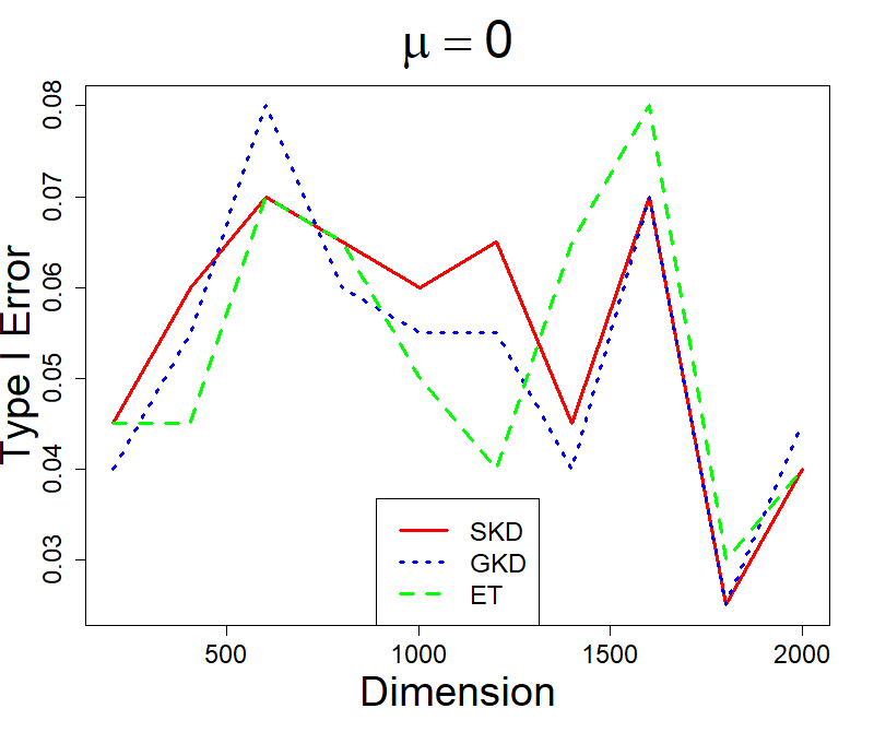
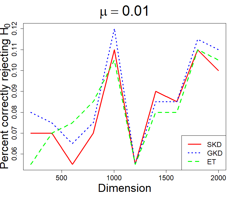
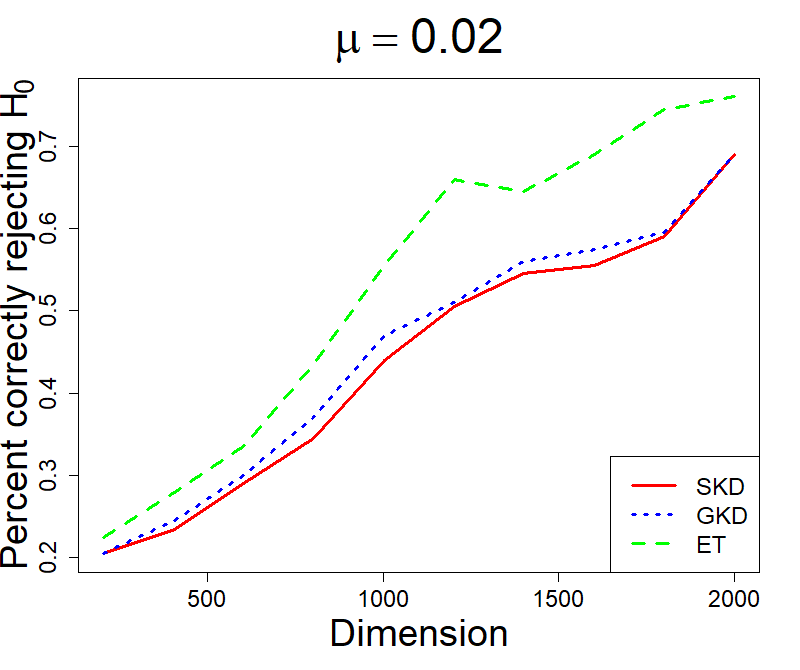
Figure 1: Perfomance of SKD, GKD, and ET under Model 1.1 with $\alpha=0.05$. Three values of $\mu$ are shown: $0$ (null hypothesis), $0.01$ and $0.02$ (alternative hypothesis).

Outputs from Model 1.1 are displayed in Figure 1. Tests calibration (i.e., the behaviour of the different tests under $\text{H}_{0}$) corresponds to the case $\mu=0$. Under the alternative hypothesis $\mu=0.01$ there is a lot of oscillation around the value $0.085$ (percentage of rejection). This is not surprising since this alternative hypothesis is close to the null. When $\mu=0.02$, we observe that the power of the three methods increases with dimension, with a faster growth for ET. This is a kind of dimension blessing and it has been observed before for kernel distances in [Gretton et al., 2008, Section 8.1]. Note also that the SKD and the GKD test (the latter with a data-driven choice of the parameter) have a very similar performance.

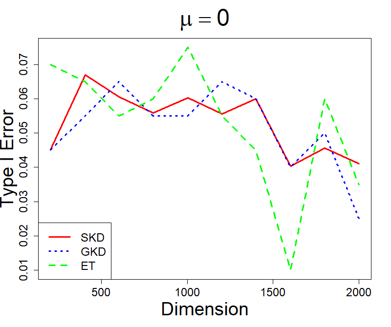
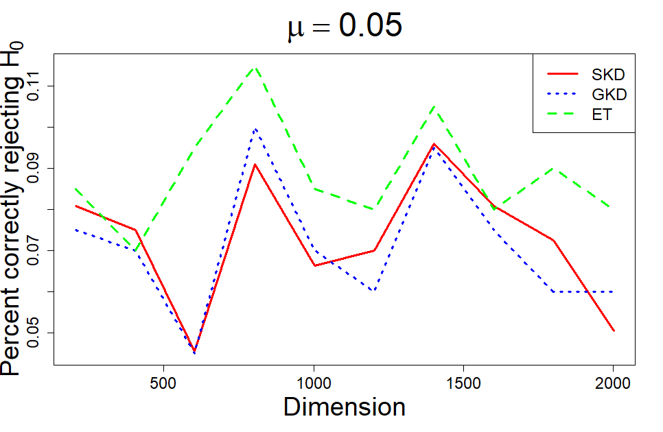
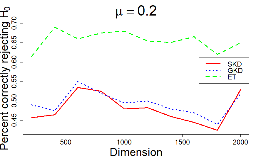
Figure 2: Perfomance of SKD, GKD, and ET under Model 1.2 with $\alpha=0.05$. Three values of $\mu$ are shown: $0$ (null hypothesis), $0.05$ and $0.2$ (alternative hypothesis).

Results of Model 1.2 can be seen in Figure 2. Test calibration outputs are depicted when $\mu=0$. As in the previous example, the second graph $\mu=0.05$ shows a relatively small power for all test, since both distributions are very close to each other. An obvious gain in power (with some advantage for ET) is observed in the case $\mu=0.2$. The functional nature of the data is apparent in the fact that there is no clear pattern of “dimensionality blessing” associated with the increase of grid size. Indeed, unlike the other examples we are considering, the use of higher dimensional observations (i.e., the use of a denser grid) does not entail a true gain in information, as the grid observations are correlated, due to the continuity of the trajectories. The ET test seems to perform better in this model and the two kernel based tests have a similar behaviour.

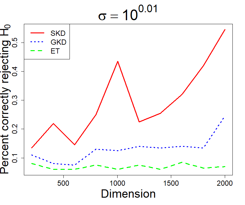
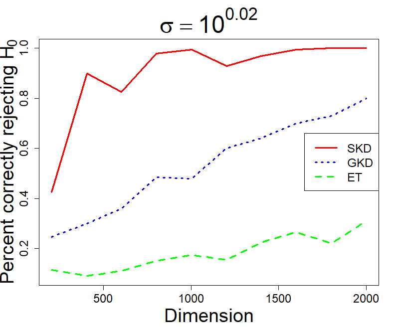
Figure 3: Perfomance of SKD, GKD, and ET under Model 2.1 with $\alpha=0.05$. Two values of $\sigma^{2}$ are shown: $10^{0.01}$ and $10^{0.02}$ (alternative hypothesis).

The outputs from the heteroscedastic Model 2.1 are placed in Figure 3. The most remarkable conclusion here is the good behaviour of the SKD test which, in particular, outperforms GKD. A plausible explanation for this difference is the fact that the median-based selection of $\lambda$ is not a good choice for the heteroscedastic case when the value of the location parameter is the same in both populations. It is also apparent, that this heteroscedastic, same-location, scenario is not the most favorable for the ET test.

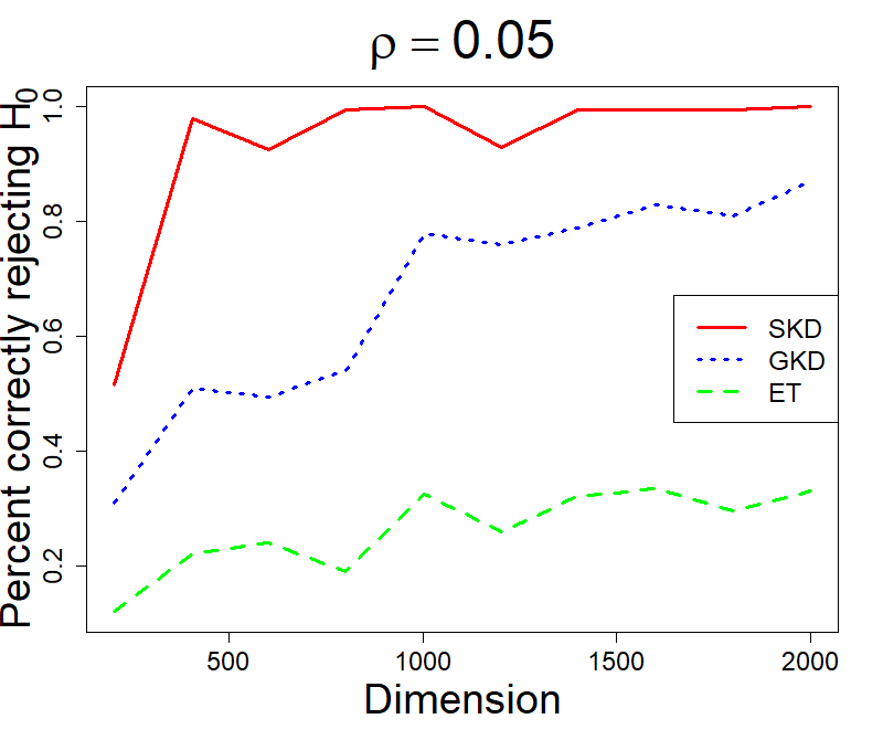
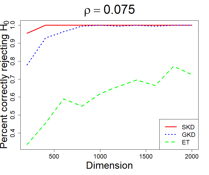
Figure 4: Perfomance of SKD, GKD, and ET under Model 2.2 with $\alpha=0.05$. Two values of $\rho$ are shown: $0.05$ and $0.075$ (alternative hypothesis).

Results of Model 2.2 are shown in Figure 4. In this model the conclusions are similar to those of Model 2.1. Note that SKD and GKD are particularly sensitive to dependence since a correlation of $\rho=0.05$ generates a power close to $1$ even in low dimension.

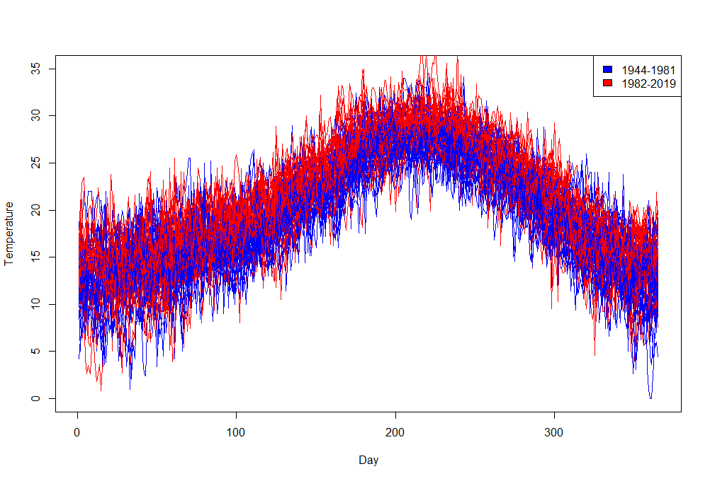
Figure 5: Maximum daily land surface temperature measured at El Prat Airport (Barcelona, Spain) between 1944 and 2019.

Finally, regarding the real data example, all the considered tests give a nearly null $p$-value. This is hardly surprising, in view of Figure 5, where the temperature curves are displayed (the red curves corresponding to the earlier period). While this is just a small, partial experiment, presented here for simple illustration purposes, the results are consistent with those of many other deeper analysis published in recent years.

Conclusions

In the light of the results, we can conclude that, globally, the supremum kernel distance test (SKD) performs at least as well as the proposal by [Gretton et al., 2008], GKD. The Energy Test (ET) of [Szekely & Rizzo, 2017] works better when the difference between the distributions lies in the location parameter. In the heteroscedastic case SKD obtains the best results. A possible explanation for this is that kernel distances are not based in the estimation of a correlation matrix. A more complete study (including derivation of the asymptotic distribution for the case of a data-driven selection of $\lambda$, the use of Pearson curves and/or modified bootstrap schemes, …) might be worthwhile in the future.

5 Proofs of the main results

We need two auxiliar lemmata to prove Theorem 1. The first result corresponds to [Marcus, 1985, Theorem 1.1].

Lemma 5.

Let $H$ be a real and separable Hilbert space. Let us consider a linear and continuous operator $T:H\rightarrow C_{b}({\mathcal{X}})$, where $C_{b}({\mathcal{X}})$ is the space of real bounded continuous functions on ${\mathcal{X}}$ endowed with the supremum norm. If $B_{H}$ is the unit ball in $H$, then the class $B=T(B_{H})$ is universal Donsker.

We also require Aronszajn’s inclusion theorem; see [Aronszajn, 1950, Theorem I].

Lemma 6.

Let $k_{1}$ and $k_{2}$ be two kernels on $\mathcal{X}$. Then, $\mathcal{H}_{k_{1}}\subset\mathcal{H}_{k_{2}}$ if and only if there exists a constant $c>0$ such that $c\,k_{2}-k_{1}$ is a positive definite kernel (i.e., $k_{1}\ll c\,k_{2}$). In such a case, we also have that $\|f\|_{\mathcal{H}_{k_{2}}}\leq\sqrt{c}\|f\|_{\mathcal{H}_{k_{1}}}$, for all $f\in\mathcal{H}_{k_{1}}$.

Proof of Theorem 1.

The first part can be seen as a consequence of Lemma 5. First, by [Berlinet & Thomas-Agnan, 2011, Theorem 17], the functions in $\mathcal{H}_{k}$ are continuous. In particular, using [Berlinet & Thomas-Agnan, 2011, Corollary 3], we conclude that $\mathcal{H}_{k}$ is a separable Hilbert space. On the other hand, for $x\in\mathcal{X}$, by the reproducing property (6) of $k$ (twice) and Cauchy–Schwarz inequality, we have that

$$\begin{split}|f(x)-g(x)|&=|\langle f-g,k(x,\cdot)\rangle_{\mathcal{H}_{k}}|\\ &\leq\|f-g\|_{\mathcal{H}_{k}}\|k(x,\cdot)\|_{\mathcal{H}_{k}}\\ &=\|f-g\|_{\mathcal{H}_{k}}\sqrt{k(x,x)}.\end{split}$$ (19)

Therefore, as $k$ is bounded on the diagonal, convergence in the RKHS norm entails uniform convergence. Further, from (19) we also see that the functions in ${\mathcal{H}}_{k}$ are bounded and hence ${\mathcal{H}}_{k}\subset C_{b}({\mathcal{X}})$. Now, we can apply Lemma 5 to $H={\mathcal{H}}_{k}$ and $T=I$, the inclusion map given by $I(f)=f$. According to (19), this linear transformation is continuous. As $B_{H}=\mathcal{F}_{k}$, by Lemma 5, we thus conclude that $\mathcal{F}_{k}=T(\mathcal{F}_{k})$ is universal Donsker.

The second part is a by-product of the first one together with Aronszajn’s inclusion theorem. According to Lemma 6, we have that $\|f\|_{{\mathcal{H}}_{k}}\leq\sqrt{c}\|f\|_{\mathcal{H}_{k,\lambda}}$, for all $f\in{\mathcal{H}}_{k,\lambda}$ and for all $\lambda\in\Lambda$. Therefore, $\mathcal{F}_{k,\Lambda}\subset\sqrt{c}\,\mathcal{F}_{k}$. Finally, from the first part of the theorem, the set $\sqrt{c}\,\mathcal{F}_{k}$ is universal Donsker as it is the unit ball of the RKHS generated by the kernel $ck$. Therefore, $\mathcal{F}_{k,\Lambda}$ is also universal Donsker (see [van der Vaart & Wellner, 1996, Theorem 2.10.1]) and the proof is complete. ∎

To prove Theorem 2, we need the following Karhunen-Loève-type result for the $\mathcal{F}_{k,\lambda}$-indexed Brownian bridge.

Lemma 7.

Under the assumptions of Theorem 2, we have that:

1. For each $\lambda\in\Lambda$, the $\mathcal{F}_{k,\lambda}$-indexed Brownian bridge $\mathbb{G}_{\text{\rm P}}$ can be extended almost surely to a continuous and linear map on $\mathcal{H}_{k,\lambda}$. Therefore, $\mathbb{G}_{\text{\rm P}}$ can be seen as a random element of the dual space $\mathcal{H}^{\ast}_{k,\lambda}$. For simplicity we also denote this extension in $\mathcal{H}^{\ast}_{k,\lambda}$ as $\mathbb{G}_{\mathrm{P}}$.

2. As an element of $\mathcal{H}^{\ast}_{k,\lambda}$, $\mathbb{G}_{\text{\rm P}}$ admits the following representation:

   $$\mathbb{G}_{\text{\rm P}}=_{\operatorname{a.s.}}\sum_{j\in\mathbb{N}}Z_{j,\lambda}\,\varphi_{j,\lambda},\quad\text{in }\mathcal{H}_{k,\lambda}^{\ast}.$$ (20)

   In particular, we have that

   $$\left\|\mathbb{G}_{\text{\rm P}}\right\|_{\mathcal{H}_{k,\lambda}^{\ast}}^{2}=_{\operatorname{a.s.}}\sum_{j\in\mathbb{N}}Z_{j,\lambda}^{2}.$$ (21)

Proof.

To show part (a), we note that, from Theorem 1, $\mathcal{F}_{k,\lambda}$ is a P-Donsker class and hence P-pre-Gaussian. Hence, by [Giné & Nickl, 2016, Theorem 3.7.28], for almost all $\omega$, the function $f\mapsto\mathbb{G}_{\text{\rm P}}(\omega)f$ ($f\in\mathcal{F}_{k,\lambda}$) is prelinear and can be uniquely extended to a linear map on $\operatorname{span}\left(\mathcal{F}_{k,\lambda}\right)=\mathcal{H}_{k,\lambda}$. Moreover, this extension is bounded and uniformly $d_{\text{\rm P}}$-continuous in $\mathcal{H}_{k,\lambda}$, where $d_{\text{\rm P}}$ is the intrinsic $\mathrm{L}^{2}(\text{\rm P})$ metric of the process. Finally, we observe that, thanks to (19),

$$d^{2}_{\text{\rm P}}(f,g)=\mathbb{E}_{\text{\rm P}}(f-g)^{2}\leq\|f-g\|_{\mathcal{H}_{k,\lambda}}^{2}\int_{\mathcal{X}}k(x,x)\,\text{\rm d}\text{\rm P}(x).$$ (22)

As by hypothesis $k$ is bounded on the diagonal, we have that uniformly $d_{\text{\rm P}}$-continuous functions on $\mathcal{H}_{k,\lambda}$ are also uniformly continuous functions with respect of the norm in $\mathcal{H}_{k,\lambda}$. In particular, $\mathbb{G}_{\text{\rm P}}$ is almost surely a continuous and linear functional on $\mathcal{H}_{k,\lambda}$, and thus an element of $\mathcal{H}^{\ast}_{k,\lambda}$. This finishes the proof of part (a).

To prove part (b) we first note that, by (a), $\mathbb{G}_{\text{\rm P}}$ is a Gaussian process in the Hilbert space $\mathcal{H}_{k,\lambda}^{\ast}$. The covariance operator $\mathcal{K}_{\mathbb{G}_{\text{\rm P}}}$ of $\mathbb{G}_{\text{\rm P}}$ is self-adjoint and compact. By the Fernique’s theorem [Bogachev, 1998, p. 74], $\mathbb{G}_{\text{\rm P}}$ is Bochner square-integrable, $\mathcal{K}_{\mathbb{G}_{\text{\rm P}}}$ is a trace-class operator and

$$\operatorname{trace}\left(\mathcal{K}_{\mathbb{G}_{\text{\rm P}}}\right)=\int_{\mathcal{H}_{k,\lambda}^{\ast}}\|z\|_{\mathcal{H}_{k,\lambda}^{\ast}}^{2}\,\mathrm{d}\nu_{\mathbb{G}_{\text{\rm P}}}(z)=\mathbb{E}\left(\left\|\mathbb{G}_{\text{\rm P}}\right\|_{\mathcal{H}_{k,\lambda}^{\ast}}^{2}\right),$$ (23)

where $\nu_{\mathbb{G}_{\text{\rm P}}}$ is the measure induced by the process $\mathbb{G}_{\text{\rm P}}$ in $\mathcal{H}_{k,\lambda}^{\ast}$. The proof of (23) can be found in [Bogachev, 1998, p. 48].

Now, by the spectral theorem, there exists $\left\{\left(\beta_{j,\lambda},\varphi_{j,\lambda}\right)\right\}_{j\in\mathbb{N}}\in\left([0,\infty)\times\mathcal{H}_{k,\lambda}^{\ast}\right)^{\mathbb{N}}$ such that $\beta_{1,\lambda}\geq\beta_{2,\lambda}\geq\cdots$; $\mathcal{K}_{\mathbb{G}_{P}}\,\varphi_{j,\lambda}=\beta_{j,\lambda}\,\varphi_{j,\lambda}$, for $j\in\mathbb{N}$; and $\left\langle\varphi_{j_{1},\lambda},\varphi_{j_{2},\lambda}\right\rangle_{\mathcal{H}_{k,\lambda}^{\ast}}=\delta_{j_{1}\,j_{2}}$, for $j_{1},j_{2}\in\mathbb{N}$ with $\delta_{i\,j}$ the Kronecker’s delta. As $\mathcal{K}_{\mathbb{G}_{\text{\rm P}}}$ is trace-class, we also have that

$$\operatorname{trace}\left(\mathcal{K}_{\mathbb{G}_{P}}\right)=\sum_{j\in\mathbb{N}}\beta_{j,\lambda}.$$

Additionally,

$$\mathbb{E}\left(\left\langle\mathbb{G}_{\text{\rm P}},\varphi_{j,\lambda}\right\rangle_{\mathcal{H}_{k,\lambda}^{\ast}}\right)=0\quad\text{and}\quad\mathbb{E}\left(\left\langle\mathbb{G}_{\text{\rm P}},\varphi_{j,\lambda}\right\rangle_{\mathcal{H}_{k,\lambda}^{\ast}}^{2}\right)=\left\langle\mathcal{K}_{\mathbb{G}_{\text{\rm P}}}\left(\varphi_{j,\lambda}\right),\varphi_{j,\lambda}\right\rangle_{\mathcal{H}_{k,\lambda}^{\ast}}=\beta_{j,\lambda}.$$ (24)

From (24), we have that $Z_{j,\lambda}=\left\langle\mathbb{G}_{\text{\rm P}},\varphi_{j,\lambda}\right\rangle_{\mathcal{H}_{k,\lambda}^{\ast}}\sim\mathcal{N}\left(0,\beta_{j,\lambda}\right)$ ($j\in\mathbb{N}$) are jointly Gaussian and independent.

To finish this proof of (20), by [Ledoux & Talagrand, 1991, Theorem 6.1], it is enough to show absolute mean convergence, which is a necessary and sufficient condition. First, by orthogonality, we observe that for every $J\subset\mathbb{N}$ finite, we have that

$$0\leq\left\|\mathbb{G}_{\text{\rm P}}-\sum_{j\in J}Z_{j,\lambda}\,\varphi_{j,\lambda}\right\|_{\mathcal{H}_{k,\lambda}^{\ast}}^{2}=\left\|\mathbb{G}_{\text{\rm P}}\right\|_{\mathcal{H}_{k,\lambda}^{\ast}}^{2}-\sum_{j\in J}Z_{j,\lambda}^{2}.$$

Then by (23),

$$\mathbb{E}\left(\left|\left\|\mathbb{G}_{\text{\rm P}}\right\|_{\mathcal{H}_{k,\lambda}^{\ast}}^{2}-\sum_{j\in J}Z_{j,\lambda}^{2}\right|\right)=\operatorname{trace}\left(\mathcal{K}_{\mathbb{G}_{\text{\rm P}}}\right)-\sum_{j\in J}\beta_{j,\lambda},$$ (25)

which is the remainder of a convergent series. Hence, (20) holds. As (21) follows from (20), the proof is complete. ∎

The proof of part (a) in Lemma 7 essentially follows from Theorem 1. However, part (b), where the series representation is obtained, must be discussed. Equation (20) shows the convergence of a series of functional random variables. This result looks like a standard Karhunen-Loève theorem, but some remarks should be done. The convergence of this series is on the dual space $\mathcal{H}_{k,\lambda}^{\ast}$, while Karhunen-Loève decomposition is stated classically on $\mathrm{L}^{2}$-type spaces. In fact, our decomposition in (20) can be seen as a particular case of the results in [Bay & Croix, 2017]. In [Giné & Nickl, 2016, Theorem 2.6.10] a similar decomposition is shown where the coordinates are deterministic while the basis is random, which is not useful for our purposes.

Proof of Theorem 2.

From Theorem 1, the class $\mathcal{F}_{k,\Lambda}$ is Donsker and hence we have that

$$\mathbb{G}_{n,m}=\sqrt{\frac{n\,m}{n+m}}\,\left(\mathbb{P}_{n}-\mathbb{Q}_{m}\right)\rightsquigarrow\mathbb{G}_{\text{\rm P}},\quad\text{in }\ell^{\infty}\left(\mathcal{F}_{k,\Lambda}\right).$$ (26)

Note that $d_{k,\Lambda}$ is the metric induced by the supremum norm in $\ell^{\infty}\left(\mathcal{F}_{k,\Lambda}\right)$, hence $d_{k,\Lambda}$ is a continuous functional. From (26) and by the continuous mapping theorem (see, for instance [van der Vaart & Wellner, 1996, Theorem 1.9.5]), we obtain that

$$\sqrt{\frac{n\,m}{n+m}}\,d_{k,\Lambda}\left(\mathbb{P}_{n},\mathbb{Q}_{m}\right)\rightsquigarrow\underset{\mathcal{F}_{k,\Lambda}}{\operatorname{sup}}\left(\mathbb{G}_{\text{\rm P}}\right).$$ (27)

From Lemma 7, the limit in (27) can be rewritten as

$$\underset{\mathcal{F}_{k,\Lambda}}{\operatorname{sup}}\left(\mathbb{G}_{\mathrm{P}}\right)=\underset{\lambda\in\Lambda}{\operatorname{sup}}\left(\underset{\mathcal{F}_{k,\lambda}}{\operatorname{sup}}\left(\mathbb{G}_{\mathrm{P}}\right)\right)=\underset{\lambda\in\Lambda}{\operatorname{sup}}\left(\left\|\mathbb{G}_{\mathrm{P}}\right\|_{\mathcal{H}_{k,\lambda}^{\ast}}\right).$$ (28)

Finally, from (28) and (21) we obtain the representation of the limit as in (13) and the proof of the theorem is complete. ∎

The next goal is to prove Corollary 4 as preparation for the proof of Theorem 3. We need a differentiability result for the supremum similar to those obtained in [Cárcamo et al., 2020]. Given a kernel $k$, we consider the mapping

$$\sigma_{k}(g)=\sup_{f\in\mathcal{F}_{k}}g(f),\quad\text{for }g\in\ell^{\infty}(\mathcal{F}_{k}),$$ (29)

where $\mathcal{F}_{k}$ is the unit ball as in (9). Observe that, by (3) and (10), if $\text{\rm P},\text{\rm Q}\in\mathcal{M}_{\operatorname{p}}(\mathcal{X})$ such that their mean embeddings $\mu_{\text{\rm P}}$ and $\mu_{\text{\rm Q}}$ exist, we have that

$$\sigma_{k}(\mathrm{P}-\mathrm{Q})=d_{k}(\mathrm{P},\mathrm{Q})=\left\|\mu_{\mathrm{P}}^{\lambda}-\mu_{\mathrm{Q}}^{\lambda}\right\|_{\mathcal{H}_{k}}.$$ (30)

The proof of Corollary 4 relies on Theorem 1 together with the differentiability properties of the mapping $\sigma_{k}$ in (29). Same ideas are used below in the proof of Theorem 3 using the mapping

$$\sigma_{k,\Lambda}(g)=\sup_{f\in\mathcal{F}_{k,\Lambda}}g(f),\quad\text{for }g\in\ell^{\infty}(\mathcal{F}_{k,\Lambda}),$$ (31)

where $\mathcal{F}_{k,\Lambda}$ is the union of balls in (11). These differentiability results might have independent interest as it can be applied in other contexts by means of the (extended) functional Delta method; see the examples in [Cárcamo et al., 2020].

The next corollary shows that $\sigma_{k}$ in (29) is fully Hadamard differentiable under some assumptions. For the precise definitions we refer to [Cárcamo et al., 2020] and the references therein.

Lemma 8.

Let us consider $\text{\rm P},\text{\rm Q}\in\mathcal{M}_{\operatorname{p}}(\mathcal{X})$ such that their mean embeddings $\mu_{\text{\rm P}}$ and $\mu_{\text{\rm Q}}$ exist and $\mu_{\text{\rm P}}\neq\mu_{\text{\rm Q}}$. We have that the mapping $\sigma_{k}$ in (29) is (fully) Hadamard differentiable at $\text{\rm P}-\text{\rm Q}$ tangentially to $\mathcal{C}(\mathcal{F}_{k},d_{\mathcal{H}_{k}})\equiv$ the subset of $\ell^{\infty}(\mathcal{F}_{k})$ constituted by continuous functionals with the RKHS norm. In such a case, the derivative of $\sigma_{k}$ at the point $\text{\rm P}-\text{\rm Q}$ is given by

$$\sigma^{\prime}_{k;\text{\rm P}-\text{\rm Q}}(g)=g(h^{+}),\quad\text{for }g\in\mathcal{C}(\mathcal{F}_{k},d_{\mathcal{H}_{k}}),$$ (32)

where $h^{+}\in\mathcal{F}_{k}$ is defined in (18).

Proof.

From [Cárcamo et al., 2020, Theorem 2.1], we have that $\sigma_{k}$ is Hadamard directionally differentiable and

$$\sigma_{k;\mathrm{P}-\mathrm{Q}}^{\prime}(g)=\underset{\varepsilon\searrow 0}{\operatorname{lim}}\,\underset{A_{\varepsilon}(\mathrm{P}-\mathrm{Q})}{\operatorname{sup}}\,(g),\quad g\in\ell^{\infty}\left(\mathcal{F}_{k}\right),$$ (33)

where

$$A_{\varepsilon}(\mathrm{P}-\mathrm{Q})=\left\{h\in\mathcal{F}_{k}:(\mathrm{P}-\mathrm{Q})\,(h)\geq d_{k}(\mathrm{P},\mathrm{Q})-\varepsilon\right\}.$$

We first check that if $h_{\varepsilon}\in A_{\varepsilon}(\mathrm{P}-\mathrm{Q})$, then $h_{\varepsilon}\to h^{+}$ in $\mathcal{H}_{k}$ as $\varepsilon\to 0$, with $h^{+}$ in (18). To see this, we first note that

$$\|h_{\varepsilon}-h^{+}\|_{\mathcal{H}_{k}}^{2}=1+\|h_{\varepsilon}\|_{\mathcal{H}_{k}}^{2}-\frac{2}{\|\mu_{\text{\rm P}}-\mu_{\text{\rm Q}}\|_{\mathcal{H}_{k}}}\left\langle h_{\varepsilon},\mu_{\text{\rm P}}-\mu_{\text{\rm Q}}\right\rangle_{\mathcal{H}_{k}}.$$ (34)

As $h_{\varepsilon}\in A_{\varepsilon}(\mathrm{P}-\mathrm{Q})$, from (8) and (30), we obtain that

$$\text{\rm P}(h_{\varepsilon})-\text{\rm Q}(h_{\varepsilon})=\left\langle h_{\varepsilon},\mu_{\text{\rm P}}-\mu_{\text{\rm Q}}\right\rangle_{\mathcal{H}_{k}}\geq\|\mu_{\text{\rm P}}-\mu_{\text{\rm Q}}\|_{\mathcal{H}_{k}}-\varepsilon.$$ (35)

Finally, from (34), (35), and as $h_{\varepsilon}\in\mathcal{F}_{k}$, we have that

$$\|h_{\varepsilon}-h^{+}\|_{\mathcal{H}_{k}}^{2}\leq\frac{2\varepsilon}{\|\mu_{\text{\rm P}}-\mu_{\text{\rm Q}}\|_{\mathcal{H}_{k}}},$$ (36)

and hence $h_{\varepsilon}\to h^{+}$ in $\mathcal{H}_{k}$ (as $\varepsilon\to 0$).

Now, we check that $\sigma^{\prime}_{k;\text{\rm P}-\text{\rm Q}}(g)=g(h^{+})$, for $g\in\mathcal{C}(\mathcal{F}_{k},d_{\mathcal{H}_{k}})$. We firstly observe that $h^{+}\in A_{\varepsilon}(\text{\rm P}-\text{\rm Q})$, for all $\varepsilon>0$. Hence, from equation (33), we have that $g(h^{+})\leq\sigma^{\prime}_{k;\text{\rm P}-\text{\rm Q}}(g)$. On the other hand, we can extract a maximizing sequence $h_{m}\in A_{1/m}(\text{\rm P}-\text{\rm Q})$ ($m\in\mathbb{N}$) satisfying that $\sup_{A_{1/m}(\text{\rm P}-\text{\rm Q})}g\leq g(h_{m})+1/m$. As $g$ is continuous and $h_{m}\to h^{+}$ as $m\to\infty$ in $\mathcal{H}_{k}$, we obtain that

$$\sigma^{\prime}_{k,\text{\rm P}-\text{\rm Q}}(g)=\lim_{m\to\infty}\sup_{A_{1/m}(\text{\rm P}-\text{\rm Q})}g\leq\lim_{m\to\infty}g(h_{m})=g(h^{+}).$$

Therefore, we obtain that $\sigma^{\prime}_{k;\text{\rm P}-\text{\rm Q}}(g)=g(h^{+})$, which is a linear mapping, so $\sigma_{k}$ is fully differentiable and the proof is complete. ∎

Proof of Corollary 4.

From Theorem 1, we have that

$$\mathbb{G}_{n,m}=\sqrt{\frac{n\,m}{n+m}}\,\left(\mathbb{P}_{n}-\mathbb{Q}_{m}-(\mathrm{P}-\mathrm{Q})\right)\rightsquigarrow\mathbb{G}=\sqrt{1-\theta}\,\mathbb{G}_{\mathrm{P}}-\sqrt{\theta}\,\mathbb{G}_{\mathrm{Q}},\quad\text{in }\ell^{\infty}\left(\mathcal{F}_{k}\right).$$ (37)

From (30), the statistic in the right-hand side of equation (17) is precisely

$$\sqrt{\frac{n\,m}{n+m}}\,\left(\sigma_{k}\left(\mathbb{P}_{n}-\mathbb{Q}_{m}\right)-\sigma_{k}(\mathrm{P}-\mathrm{Q})\right),$$ (38)

where $\sigma_{k}$ is defined in (29).

Using the same ideas as in the proof of [Cárcamo et al., 2020, Theorem 6.1], it can be checked that the paths of $\mathbb{G}$ in (37) are a.s. in $\mathcal{C}_{u}(\mathcal{F}_{k},\rho)$ (uniformly continuous), where

$$\rho=\operatorname{max}\left(d_{\mathrm{L}^{2}(\mathrm{P})},d_{\mathrm{L}^{2}(\mathrm{Q})}\right)$$ (39)

is the natural $\mathrm{L}^{2}$-metric of $\mathbb{G}$. From (22), it can be readily checked that $\mathcal{C}_{u}(\mathcal{F}_{k},\rho)\subset\mathcal{C}_{u}(\mathcal{F}_{k},d_{\mathcal{H}_{k}})$ and hence $\mathbb{G}\in\mathcal{C}(\mathcal{F}_{k},d_{\mathcal{H}_{k}})$ a.s. To finish the proof it is enough to apply Lemma 8 together with the functional Delta method [van der Vaart & Wellner, 1996, Section 3.9]. ∎

To prove Theorem 3 we need the following key lemma.

Lemma 9.

Let us assume that the family of kernels $\{k_{\lambda}:\lambda\in\Lambda\}$ satisfies 3, 3 and 3. If $\text{\rm P},\text{\rm Q}\in\mathcal{M}_{\operatorname{p}}(\mathcal{X})$ such that $\text{\rm P}\neq\text{\rm Q}$, then the mapping $\sigma_{k,\Lambda}$ in (31) is Hadamard directionally differentiable at $\text{\rm P}-\text{\rm Q}$ tangentially to $\mathcal{C}(\mathcal{F}_{k,\Lambda},\rho)\equiv$ the subset of $\ell^{\infty}(\mathcal{F}_{k,\Lambda})$ constituted by continuous functionals with respect to the distance $\rho$ in (39). In such a case, the (directional) derivative of $\sigma_{k,\Lambda}$ at the point $\text{\rm P}-\text{\rm Q}$ is given by

$$\sigma_{k,\Lambda;\mathrm{P}-\mathrm{Q}}^{\prime}(g)=\underset{\lambda\in\Lambda_{0}}{\operatorname{sup}}\left(g\left(h^{+,\lambda}\right)\right)=\underset{L}{\operatorname{sup}}\,(g),\quad g\in\mathcal{C}(\mathcal{F}_{k,\Lambda},\rho),$$ (40)

where the functions $h^{+,\lambda}$ are defined in (15) and the sets $\Lambda_{0}$ and $L$ in (16).

Proof.

Let us fix $g\in\mathcal{C}(\mathcal{F}_{k,\Lambda},\rho)$. Again, from [Cárcamo et al., 2020, Theorem 2.1], we have that $\sigma_{k,\Lambda}$ is Hadamard directionally differentiable and

$$\sigma_{k,\Lambda;\mathrm{P}-\mathrm{Q}}^{\prime}(g)=\underset{\varepsilon\searrow 0}{\operatorname{lim}}\,\underset{A_{\varepsilon,\Lambda}(\mathrm{P}-\mathrm{Q})}{\operatorname{sup}}\,(g),$$ (41)

where

$$A_{\varepsilon,\Lambda}(\mathrm{P}-\mathrm{Q})=\left\{h\in\mathcal{F}_{k,\Lambda}:(\mathrm{P}-\mathrm{Q})\,(h)\geq d_{k,\Lambda}(\mathrm{P},\mathrm{Q})-\varepsilon\right\}.$$

For every $\varepsilon>0$, it is clear that $L\subseteq A_{\varepsilon,\Lambda}(\mathrm{P}-\mathrm{Q})$, where $L$ is defined in (16). Hence, we have that

$$\underset{\lambda\in\Lambda_{0}}{\operatorname{sup}}\left(g\left(h^{+,\lambda}\right)\right)\leq\sigma_{k,\Lambda;\mathrm{P}-\mathrm{Q}}^{\prime}(g).$$ (42)

Conversely, we consider a maximizing sequence $(h_{m})_{m\in\mathbb{N}}$ satisfying that $h_{m}\in A_{1/m,\Lambda}(\text{\rm P}-\text{\rm Q})$ and

$$\sup_{A_{1/m,\Lambda}(\text{\rm P}-\text{\rm Q})}(g)\leq g(h_{m})+\frac{1}{m}.$$ (43)

Each $h_{m}\in\mathcal{F}_{k,\lambda_{m}}$ ($m\in\mathbb{N}$), for some $\lambda_{m}\in\Lambda$. We consider the sequence $(h^{+,\lambda_{m}})_{m\in\mathbb{N}}$. Using 3, by restricting, if needed, to a subsequence we can assume that $\lambda_{m}\to\lambda^{\star}\in\Lambda$. Next we prove the following facts:

1. $\lambda^{\star}\in\Lambda_{0}$, where $\Lambda_{0}$ is in (16), and

   $$\|\mu_{\text{\rm P}}^{\lambda_{m}}-\mu_{\text{\rm Q}}^{\lambda_{m}}\|_{\mathcal{H}_{k,\lambda_{m}}}\to\|\mu_{\text{\rm P}}^{\lambda^{\star}}-\mu_{\text{\rm Q}}^{\lambda^{\star}}\|_{\mathcal{H}_{k,\lambda^{\star}}}=d_{k,\Lambda}(\text{\rm P},Q)>0.$$ (44)

2. $\rho(h_{m},h^{+,\lambda_{m}})\to 0$, as $m\to\infty$.

3. $\rho(h_{m},h^{+,\lambda^{\star}})\to 0$, as $m\to\infty$.

First, (44) is obtained by using the representation of the kernel distance as a double integral in (3), together with 3, 3 and the dominated convergence theorem (DCT). Further, as $h_{m}\in\mathcal{F}_{k,\lambda_{m}}\cap A_{1/m,\Lambda}(\text{\rm P}-\text{\rm Q})$, we obtain that

$$\|\mu_{\mathrm{P}}^{\lambda_{m}}-\mu_{\mathrm{Q}}^{\lambda_{m}}\|_{\mathcal{H}_{k,\lambda_{m}}}\geq\text{\rm P}(h_{m})-\text{\rm Q}(h_{m})\geq d_{k,\Lambda}(\text{\rm P},\text{\rm Q})-\frac{1}{m}.$$

Hence, from (44) and by taking $m\to\infty$ we obtain that $\lambda^{\star}\in\Lambda_{0}$. The fact that $d_{k,\Lambda}(\text{\rm P},Q)>0$ follows from 3 and the proof of (i) is complete.

To show (ii), using the same ideas as in the proof of equation (36) and (i), we obtain that

$$\|h_{m}-h^{+,\lambda_{m}}\|^{2}_{\mathcal{H}_{k,\lambda_{m}}}\leq 2-\frac{2d_{k,\Lambda}(\text{\rm P},\text{\rm Q})-1/m}{\|\mu_{\mathrm{P}}^{\lambda_{m}}-\mu_{\mathrm{Q}}^{\lambda_{m}}\|_{\mathcal{H}_{k,\lambda_{m}}}}\to 0,\quad\text{as }m\to\infty.$$

Now, from (22) and 3, we have that

$$d^{2}_{\text{\rm P}}(h_{m},h^{+,\lambda_{m}})^{2}\leq\|h_{m}-h^{+,\lambda_{m}}\|^{2}_{\mathcal{H}_{k,\lambda_{m}}}c\int_{\mathcal{X}}k(x,x)\,\text{\rm d}\text{\rm P}(x)\to 0,\quad\text{as }m\to\infty.$$

Therefore, $\rho(h_{m},h^{+,\lambda_{m}})\to 0$, and (ii) holds.

To check (iii), by (ii), it is enough to see that $\rho(h^{+,\lambda_{m}},h^{+,\lambda^{\star}})\to 0$, as $m\to\infty$. By (44) and repeatedly applying DCT (thanks to 3), it can be checked that

$$h^{+,\lambda_{m}}(x)\to h^{+,\lambda^{\star}}(x),\quad\text{as $m\to\infty$ and for all }x\in\mathcal{X}.$$

Furthermore, for $m$ large enough, we have that

$$|h^{+,\lambda_{m}}(x)|\leq\frac{2c(|\mu_{\text{\rm P}}(x)|+|\mu_{\text{\rm Q}}(x)|)}{d_{k,\Lambda}(\text{\rm P},Q)}\in\mathrm{L}^{2}(\text{\rm P}),$$

where $\mu_{\text{\rm P}}$ and $\mu_{\text{\rm Q}}$ are the mean embeddings corresponding to the dominating kernel $k$ in 3. Hence, we can apply one more time DCT to obtain that $d_{\text{\rm P}}(h^{+,\lambda_{m}},h^{+,\lambda^{\star}})\to 0$. This implies that $\rho(h^{+,\lambda_{m}},h^{+,\lambda^{\star}})\to 0$, as $m\to\infty$.

To finish, we use (43), (i), (iii), as well as the continuity of the functional $g$ (with respect to the metric $\rho$) to obtain that

$$\sigma_{k,\Lambda;\mathrm{P}-\mathrm{Q}}^{\prime}(g) =\underset{m\to\infty}{\operatorname{lim}}\,\underset{A_{1/m,\Lambda}(\mathrm{P}-\mathrm{Q})}{\operatorname{sup}}\,(g)$$

$$\leq\underset{m\rightarrow\infty}{\operatorname{lim}}g\left(h_{m}\right)=g\left(h^{+,\lambda^{\star}}\right)$$

$$\leq\underset{\lambda\in\Lambda_{0}}{\operatorname{sup}}\left(g\left(h^{+,\lambda}\right)\right)=\underset{L}{\operatorname{sup}}\,(g).$$

The conclusion of this lemma follows from (42) and the previous inequalities. ∎

Proof of Theorem 3.

The proof of this theorem is analogous to that of Corollary 4 using Lemma 9 instead of Lemma 8. Details are ommited. ∎

Appendix

We collect here some technical results on the existence of the mean embedding in (1). Throughout this appendix $(\mathcal{X},\tau)$ is a topological space. We start with the formal definition of this concept.

Definition 10.

Let $\left(\mathcal{H}_{k},\left\langle\cdot,\cdot\right\rangle_{\mathcal{H}_{k}}\right)$ be a RKHS on $\mathcal{X}$ and let $\mathrm{P}$ be a Borel probability measure on $(\mathcal{X},\tau)$. The mean embedding of $\mathrm{P}$ is an element $\mu_{\mathrm{P}}\in\mathcal{H}_{k}$ such that $\mathrm{P}(f)=\left\langle f,\mu_{\mathrm{P}}\right\rangle_{\mathcal{H}_{k}}$, for all $f\in\mathcal{H}_{k}$.

The mean embedding has been used in [Berlinet & Thomas-Agnan, 2011, Chapter 4] and the references therein to induce a Hilbert space structure in the set of probability measures. A review of various applications of the mean embedding in statistics can be found in [Smola et al., 2007].

The mean embedding can be introduced in general Hilbert spaces. However, when the Hilbert space has a reproducing kernel the mean embedding can be expressed as the integral of a vector-valued function. This is the reason why it is called “mean” and not just embedding. The extension of the Lebesgue integral to vector-valued functions is carried out in two ways: Bochner or strong integral and Pettis or weak integral; see [Hille & Phillips, 1957, Chapter III] for further details. For our purposes the weak integral is suitable. Let us remind the definition, taken from [Pettis, 1938, Definition 2.1], of the weak integral.

Definition 11.

Let $\left(\mathcal{H}_{k},\left\langle\cdot,\cdot\right\rangle_{\mathcal{H}_{k}}\right)$ be a RKHS on $\mathcal{X}$ and $F:\mathcal{X}\longrightarrow\mathcal{H}_{k}$ be a weakly measurable map, that is, for every $h\in\mathcal{H}_{k}$ the function

$$\left\langle F,h\right\rangle_{\mathcal{H}_{k}}: \mathcal{X}\longrightarrow\mathbb{R}$$

$$x\longmapsto\left\langle F(x),g\right\rangle_{\mathcal{H}_{k}}$$

is Borel measurable. We say that $F$ is Pettis or weakly integrable with respect to a Borel probability measure $\mathrm{P}$ on $(\mathcal{X},\tau)$ if and only if

1. For every $h\in\mathcal{H}_{k}$, the map $\left\langle F(\cdot),h\right\rangle_{\mathcal{H}_{k}}$ belongs to $\mathrm{L}^{1}(\mathrm{P})$.

2. There exists $m_{F}\in\mathcal{H}_{k}$ such that $\left\langle m_{F},h\right\rangle_{\mathcal{H}_{k}}=\mathrm{P}\left(\left\langle F,h\right\rangle_{\mathcal{H}_{k}}\right)$, for every $h\in\mathcal{H}_{k}$.

In such a case, $m_{F}$ is called the integral of $F$ (with respect to $\mathrm{P}$).

Remark 12.

When $F(x)=k(\cdot,x)=\varphi_{x}$ is the feature mapping in Definition 11, we have that:

1. By the reproducing property, condition 1 is equivalent to $\mathcal{H}_{k}\subseteq\mathrm{L}^{1}(\mathrm{P})$.

2. By the Riesz representation theorem and the reproducing property, condition 2 is equivalent to saying that the integral operator $\mathrm{P}$ is a continuous functional on $\mathcal{H}_{k}$.

Remark 12 implies that the Pettis integrability of the feature mapping with respect to a measure is equivalent to the existence of the mean embedding of such measure. Let us now focus on the properties of Pettis integral to state necessary and sufficient conditions regarding the existence of the mean embedding of a probability measure.

Proposition 13.

Let $\left(\mathcal{H}_{k},\left\langle\cdot,\cdot\right\rangle_{\mathcal{H}_{k}}\right)$ be a RKHS on $\mathcal{X}$ and let $\mathrm{P}$ be a Borel probability measure on $(\mathcal{X},\tau)$. The following four conditions are equivalent:

1. The mean embedding of $\mathrm{P}$, $\mu_{\mathrm{P}}$, exists in $\mathcal{H}_{k}$.

2. The feature mapping $\varphi$ is Pettis integrable.

3. $\mathcal{F}_{k}$, the unit ball of $\mathcal{H}_{k}$, is $\mathrm{P}$-integrally bounded. In other words, $\underset{f\in\mathcal{F}_{k}}{\operatorname{sup}}\,(\mathrm{P}(f))<\infty$.

4. $\mathcal{H}_{k}\subseteq\mathrm{L}^{1}(\mathrm{P})$.

In any, and hence all, of these situations, $\mathrm{P}$ defines a continuous linear functional on $\mathcal{H}_{k}$ via (7) and

$$\left\|\mu_{\mathrm{P}}\right\|_{\mathcal{H}_{k}}=\|\mathrm{P}\|_{\mathcal{H}_{k}^{\ast}}=\left(\int_{\mathcal{X}}\int_{\mathcal{X}}k(x,y)\,\text{\rm d}\text{\rm P}(y)\,\text{\rm d}\text{\rm P}(x)\right)^{{}^{1}\!/_{2}},$$ (45)

where $\mathcal{H}_{k}^{\ast}$ is the dual space of $\mathcal{H}_{k}$.

Proof.

Next we show the following equivalences: 1$\Leftrightarrow$2, 2$\Leftrightarrow$3 and 2$\Leftrightarrow$4.

1$\Leftrightarrow$2.

The proof of this equivalence is a formalization of the statement of Remark 12. By definition of the feature mapping $\varphi$, we have that

$$\int_{\mathcal{X}}|f(x)|\,\mathrm{dP}(x)=\int_{\mathcal{X}}\left|\left\langle f,\varphi_{x}\right\rangle_{\mathcal{H}_{k}}\right|\,\mathrm{dP}(x),\quad f\in\mathcal{H}_{k}.$$

That is, condition 1 in Definition 11 and $\mathcal{H}_{k}\subseteq\mathrm{L}^{1}(\mathrm{P})$ are equivalent. Additionally,

$$\left\langle f,\mu_{\mathrm{P}}\right\rangle_{\mathcal{H}_{k}}=\int_{\mathcal{X}}f(x)\,\mathrm{dP}(x)=\int_{\mathcal{X}}\left\langle f,\varphi_{x}\right\rangle_{\mathcal{H}_{k}}\,\mathrm{dP}(x),\quad f\in\mathcal{H}_{k}.$$

Therefore, condition 2 in Definition 11 and the existence of the mean embedding are equivalent. In conclusion, Pettis integrability of the feature mapping $\varphi$ and the existence of the mean embedding $\mu_{\mathrm{P}}$ in $\mathcal{H}_{k}$ are equivalent.

2$\Leftrightarrow$3.

Condition 1 in Definition 11 means that $\mathrm{P}$ is well defined (as linear functional on $\mathcal{H}_{k}$). Additionally, by the Riesz’s representation theorem (see [Conway, 1994, Chapter 1, 3.4]), condition 2 in Definition 11 and the continuity of $\mathrm{P}$ are equivalent. Since $\mathrm{P}$ is linear, continuity of $\mathrm{P}$ and $\underset{f\in\mathcal{F}_{k}}{\operatorname{sup}}\,(|\mathrm{P}(f)|)<\infty$ are equivalent (see [Conway, 1994, Chapter 1, 3.1]).

2$\Leftrightarrow$4.

It is clear that, by condition 1 in Definition 11, statement 2 implies claim 4. Conversely, let us assume that $\mathcal{H}_{k}\subseteq\mathrm{L}^{1}(\mathrm{P})$, which is condition 1 in Definition 11. By [Hille & Phillips, 1957, Theorem 3.7.1], there exists $h^{\ast\ast}\in\mathcal{H}_{k}^{\ast\ast}$ (the bidual space of $\mathcal{H}_{k}$) such that for every $f\in\mathcal{H}_{k}$,

$$h^{\ast\ast}\left(\left\langle\cdot,f\right\rangle_{\mathcal{H}_{k}}\right)=\int_{\mathcal{X}}\left\langle\varphi_{x},f\right\rangle_{\mathcal{H}_{k}}\,\mathrm{dP}(x)=\int_{\mathcal{X}}f(x)\,\mathrm{dP}(x),$$

where $\left\langle\cdot,f\right\rangle_{\mathcal{H}_{k}}$ stands for the functional associated with $f$ by the Riesz’s representation theorem. Such $h^{\ast\ast}$ is unique. Since every Hilbert space is reflexive, there exists $h\in\mathcal{H}_{k}$ such that $h^{\ast\ast}\left(\left\langle\cdot,f\right\rangle_{\mathcal{H}_{k}}\right)=\left\langle h,f\right\rangle_{\mathcal{H}_{k}}$, for every $f\in\mathcal{H}_{k}$. Then condition 2 of Definition 11 holds. We conclude that $h$ is the Pettis integral of $\varphi$ with respect to $\mathrm{P}$.

Finally, equation (45) is just the expression of the norm of $\mu_{\mathrm{P}}$ deduced from the properties of the Pettis integral. ∎

We observe that conditions 1-4 in Proposition 13 always hold if

$$\int_{\mathcal{X}}\left\|\varphi_{x}\right\|_{\mathcal{H}_{k}}\,\mathrm{dP}(x)=\int_{\mathcal{X}}\sqrt{k(x,x)}\,\mathrm{dP}(x)<\infty.$$

Indeed, by Cauchy–Schwarz inequality,

$$|\mathrm{P}(f)|=\left|\int_{\mathcal{X}}\left\langle f,k(\cdot,x)\right\rangle_{\mathcal{H}_{k}}\,\mathrm{dP}(x)\right|\leq\|f\|_{\mathcal{H}_{k}}\,\int_{\mathcal{X}}\sqrt{k(x,x)}\,\mathrm{dP}(x).$$

Hence, we conclude that there exists $\mu_{\mathrm{P}}$ satisfying Definition 10. In particular, any kernel bounded on the diagonal trivially fulfills this requirement.

References

- [Aronszajn, 1950] Aronszajn, N. (1950). Theory of reproducing kernels. Transactions of the American mathematical society, 68(3), 337-404.
- [del Barrio et al., 2020] del Barrio, E., Inouzhe, H., and Matrán, C. (2020). On approximate validation of models: a Kolmogorov–Smirnov-based approach. TEST, 29(4), 938-965.
- [Bay & Croix, 2017] Bay, X., & Croix, J.-C. (2017). Karhunen-Loève decomposition of Gaussian measures on Banach spaces. https://arxiv.org/abs/1704.01448.
- [Berlinet & Thomas-Agnan, 2011] Berlinet, A., & Thomas-Agnan, C. (2011). Reproducing kernel Hilbert spaces in probability and statistics. Luxemburg: Springer Sciences & Bussiness Media.
- [Billingsley, 2013] Billingsley, P. (2013). Convergence of probability measures. John Wiley & Sons.
- [Brezis, 2010] Brezis, H. (2010). Functional analysis, Sobolev spaces and partial differential equations. New York: Springer New York.
- [Bogachev, 1998] Bogachev, V. I. (1998). Gaussian measures. Providence: American Mathematical Society.
- [Borgwardt et al., 2006] Borgwardt, K.M., Gretton, A., Rasch, M.J., Kriegel, H.P., Schölkopf, B., and Smola, A.J. (2006). Integrating structured biological data by kernel maximum mean discrepancy. Bioinformatics, 22(14), e49-e57.
- [Cárcamo et al., 2020] Cárcamo, J., Cuevas, A., & Rodríguez, L.-A. (2020). Directional differentiability for supremum-type functionals: Statistical applications. Bernoulli, 26(3), 2143–2175.
- [Conway, 1994] Conway, J. B. (1994). A course in functional analysis. New York: Springer New York.
- [Cuesta-Albertos et al., 2007] Cuesta-Albertos, J. A., Fraiman, R., and Ransford, T. (2007). A sharp form of the Cramer–Wold theorem. Journal of Theoretical Probability, 20(2), 201–209.
- [Cuevas et al., 2004] Cuevas, A., Febrero, M. & Fraiman, R. (2004). An anova test for functional data. Comput. Statist. Data Anal., 47(1), 111–-122.
- [Debnath & Mikusinski, 2005] Debnath, L., & Mikusinski, P. (2005). Introduction to Hilbert spaces with applications. Academic press.
- [Dette & Kokot, 2022] Dette, H., & Kokot, K. (2022). Detecting relevant differences in the covariance operators of functional time series: a sup-norm approach. Annals of the Institute of Statistical Mathematics, 74(2), 195-231.
- [Fang & Santos, 2019] Fang, Z., & Santos, A. (2019). Inference on directionally differentiable functions. The Review of Economic Studies, 86(1), 377-412.
- [El-Fallah, 2014] El-Fallah, O., Kellay, K., Mashreghi, J., & Ransford, T. (2014). A primer on the Dirichlet space (Vol. 203). Cambridge University Press.
- [Fukumizu et al., 2008] Fukumizu, K., Gretton, A., Sun, X., and Schölkopf, B. (2008). Kernel measures of conditional dependence. Advances in neural information processing systems, 489-496.
- [Giné & Nickl, 2008] Giné, E., and Nickl, R. (2008). Uniform central limit theorems for kernel density estimators. Probability Theory and Related Fields, 141(3), 333-387.
- [Giné & Nickl, 2016] Giné, E., and Nickl, R. (2016). Mathematical Foundations of Infinite-Dimensional Statistical Models. Cambridge Series in Statistical and Probabilistic Mathematics. Cambridge University Press.
- [Gretton et al., 2007] Gretton, A., Borgwardt, K., Rasch, M., Schölkopf, B., & Smola, A. J. (2007). A kernel method for the two-sample-problem. Advances in neural information processing systems pp. 513-520.
- [Gretton et al., 2008] Gretton, A., Fukumizu, Teo, C.H., Song, L., Schölkopf, B., and Smola, A. (2012). A kernel statistical test of independence. Advances in neural information processing systems, 585-592.
- [Gretton et al., 2012a] Gretton, A., Sejdinovic, D., Strathmann, H., Balakrishnan, S., Pontil, M., Fukumizu, K., & Sriperumbudur, B. K. (2012). Optimal kernel choice for large-scale two-sample tests. Advances in neural information processing systems (pp. 1205-1213).
- [Gretton et al., 2012b] Gretton, A., Borgwardt, K.M., Rasch, M.J., Schölkopf, B., and Smola, A. (2012). A kernel two-sample test. Journal of Machine Learning Research, 13(Mar), 723-773.
- [Hall & Van Keilegom 2007] Hall, P. and Van Keilegom, I. (2007). Two-sample tests in functional data analysis starting from discrete data. Statistica Sinica, 17(4), 151–1531.
- [Hsing & Eubank, 2015] Hsing, T., & Eubank, R. (1991). Theoretical Foundations of Functional Data Analysis, with an Introduction to Linear Operators. John Wiley & Sons.
- [Hille & Phillips, 1957] Phillips, R. S., & Hille, E. (1957). Functional analysis and semi-groups. RI.
- [Janson, 1997] Janson, S. (1997). Gaussian Hilbert Spaces. Cambridge University Press.
- [Ledoux & Talagrand, 1991] Ledoux, M., & Talagrand, M. (1991). Probability in Banach Spaces: isoperimetry and processes. Springer Science & Business Media.
- [Marcus, 1985] Marcus, D. J. (1985). Relationships between Donsker classes and Sobolev spaces. Zeitschrift für Wahrscheinlichkeitstheorie und Verwandte Gebiete, 69(3), 323-330.
- [Müller, 1997] Müller, A. (1997). Integral probability metrics and their generating classes of functions. Advances in Applied Probability, 29(2), 429-443.
- [Paulsen & Raghupathi, 2016] Paulsen, V. I., & Raghupathi, M. (2016). An introduction to the theory of reproducing kernel Hilbert spaces (Vol. 152). Cambridge University Press.
- [Pettis, 1938] Pettis, B. J. (1938). On integration in vector spaces. Transactions of the American Mathematical Society, 44(2), 277-304.
- [Pomann et al. 2016] Pomann, G. M., Staicu, A. M., and Ghosh, S. (2016). A two‐sample distribution‐free test for functional data with application to a diffusion tensor imaging study of multiple sclerosis. Journal of the Royal Statistical Society, Ser. C, , 65(3), 395–414.
- [Rachev et al., 2013] Rachev, S. T., Klebanov, L., Stoyanov, S. V., & Fabozzi, F. (2013). The methods of distances in the theory of probability and statistics. Springer Science & Business Media.
- [Rizzo & Szekely, 2022] Rizzo M, Szekely G (2022). E-Statistics: Multivariate Inference via the Energy of Data. R package version 1.7–10, https://CRAN.R-project.org/package=energy.
- [Scholkopf & Smola, 2018] Scholkopf, B., & Smola, A. J. (2018). Learning with kernels: support vector machines, regularization, optimization, and beyond. MIT press.
- [Sejdinovic et al., 2013] Scholkopf, B., Sriperumbudur, B., Gretton, A., & Fukumizu, K. (2013). Equivalence of distance-based and RKHS-based statistics in hypothesis testing. The Annals of Statistics, 2263-2291.
- [Shapiro, 1991] Shapiro, A. (1991). Asymptotic analysis of stochastic programs. Annals of Operations Research, 30(1), 169-186.
- [Smola et al., 2007] Smola, A., Gretton, A., Song, L., & Schölkopf, B. (2007, October). A Hilbert space embedding for distributions. In International Conference on Algorithmic Learning Theory (pp. 13-31). Springer, Berlin, Heidelberg.
- [Sriperumbudur et al., 2010] Sriperumbudur, B. K., Gretton, A., Fukumizu, K., Schölkopf, B., & Lanckriet, G. R. (2010). Hilbert space embeddings and metrics on probability measures. Journal of Machine Learning Research, 11(Apr), 1517-1561.
- [Sriperumbudur et al., 2011] Sriperumbudur, B.K., Fukumizu, K., & Lanckriet, G.R. (2011). Universality, characteristic kernels and RKHS embedding of measures. Journal of Machine Learning Research, 12(Jul), 2389-2410.
- [Sriperumbudur, 2016] Sriperumbudur, B. (2016). On the optimal estimation of probability measures in weak and strong topologies. Bernoulli, 22(3), 1839–1893.
- [Szekely & Rizzo, 2017] Szekely, G. J., & Rizzo, M. L. (2017). The energy of data. Annual Review of Statistics and Its Application, 4, 447-479.
- [Tukey, 1959] A quick, compact, two-sample test to Duckworth’s specifications. Technometrics, 1, 31-48.
- [van der Vaart & Wellner, 1996] van der Vaart, A.W., & Wellner, J.A. (1996). Weak Convergence and Empirical Processes: With Applications to Statistics. Springer.
- [Vapnik, 2013] Vapnik, V. (2013). The nature of statistical learning theory. Springer science & business media.
- [Wynne & Duncan, 2022] Wynne, G., & Duncan, A. B. (2022). A kernel two-sample test for functional data. Journal of Machine Learning Research, 23(73), 1–51.
- [Zhang, 2014] Zhang, J.T. (2014). Analysis of variance for functional data. Monographs on Statistics and Applied Probability, 127. CRC Press.
- [Zhang & Zhao, 2013] Zhang, H., & Zhao, L. (2013). On the inclusion relation of reproducing kernel Hilbert spaces. Analysis and Applications, 11(02), 1350014.
- [Zhang & Zhou, 2022] Zhang, J. T., Guo, J., & Zhou, B. (2022). Testing equality of several distributions in separable metric spaces: A maximum mean discrepancy based approach. Journal of Econometrics, in press.