GMMSeg: Gaussian Mixture based
Generative Semantic Segmentation Models

Abstract

Prevalent semantic segmentation solutions are, in essence, a dense discriminative classifier of $p(\text{{class}}\,|\text{{pixel${}_{\!}$ feature}})$. Though straightforward, this de facto paradigm neglects the underlying data distribution $p(\text{{pixel${}_{\!}$ feature}}\,|\text{{class}})$, and struggles to identify out-of-distribution data. Going beyond this, we propose GMMSeg, a new family of segmentation models that rely on a dense generative classifier for the joint distribution $p(\text{{pixel${}_{\!}$ feature}},\text{{class}})$. For each class, GMMSeg builds Gaussian Mixture Models (GMMs) via Expectation-Maximization (EM), so as to capture class-conditional densities. Meanwhile, the deep dense representation is end-to-end trained in a discriminative manner, i.e., maximizing $p(\text{{class}}\,|\text{{pixel${}_{\!}$ feature}})$. This endows GMMSeg with the strengths of both generative and discriminative models. With a variety of segmentation architectures and backbones, GMMSeg outperforms the discriminative counterparts on three closed-set datasets. More impressively, without any modification, GMMSeg even performs well on open-world datasets. We believe this work brings fundamental insights into the related fields.

1 Introduction

Semantic segmentation aims to explain visual semantics at the pixel level. It is typically considered as a problem of pixel-wise classification, i.e., assigning a class label $c\!\in\!\{1,_{\!}\cdots_{\!},C\}$ to each pixel data ${x}$.
Under this regime, deep-neural solutions are naturally built as a combination of two parts (Fig.${}_{\!}$ 1(a)): an encoder-decoder, dense feature extractor that maps $x$ to a high-dimensional feature representation $\bm{x}$, and a dense classifier that conducts $C$-way classification given input pixel feature $\bm{x}$. Starting from the first end-to-end segmentation solution – fully convolutional networks (FCN)${}_{\!}$ [1], researchers leave the classifier as parametric softmax, and fully devote to improving the dense feature extractor for learning better representation. As a result, a huge amount of FCN-based solutions${}_{\!}$ [2, 3, 4, 5] emerged and their state-of-the-art was further pushed forward by recent Transformer${}_{\!}$ [6]-style algorithms${}_{\!}$ [7, 8, 9, 10].

From a probabilistic perspective, the softmax classifier, supervised by the cross-entropy loss together with the feature extractor, directly models the class probability given an input, i.e., posterior $p(c|\bm{x})$.${}_{\!}$ This${}_{\!}$ is${}_{\!}$ known${}_{\!}$ as${}_{\!}$ a${}_{\!}$ discriminative${}_{\!}$ classifier,${}_{\!}$ as${}_{\!}$ the${}_{\!}$ conditional${}_{\!}$ probability${}_{\!}$ distribution${}_{\!}$ discriminates directly between the different values of $c_{\!}$ [11]. As discriminative classifiers directly find the classifica- tion rule with the smallest error rate, they often give excellent performance in downstream tasks, and hence become the de facto paradigm in segmentation. Yet, due to the discriminative nature, softmax- based${}_{\!}$ segmentation${}_{\!}$ models${}_{\!}$ suffer${}_{\!}$ from${}_{\!}$ several${}_{\!}$ limitations:${}_{\!}$ First,${}_{\!}$ they${}_{\!}$ only${}_{\!}$ learn${}_{\!}$ the${}_{\!}$ decision${}_{\!}$ boundary between classes, without modeling the underlying data distribution${}_{\!}$ [11]. Second, as only one weight vector is learned per class, they assume unimodality for each class${}_{\!}$ [12, 13], bearing no within-class variation. Third, they learn a prediction space where the model accuracy deteriorates rapidly away from the decision boundaries${}_{\!}$ [14] and thus yield poorly calibrated predictions${}_{\!}$ [15], struggling to recognize out-of-distribution data${}_{\!}$ [16]. The first two limitations may hinder the expressive power of segmentation models, and the last one challenges the adoption of segmentation models in decision-critical tasks (e.g., autonomous driving) and motivates the development of anomaly segmentation methods [17, 18, 19] (which, however, rely on pre-trained discriminative segmentation models).

Figure 1: (a) Existing softmax based discriminative regime only learns decision boundaries on the pixel embedding space. (b) Our GMMSeg models pixel feature densities via generative GMMs.

As an alternative of discriminative classifiers, generative classifiers first find the joint probability $p(\bm{x},c)$, and use $p(\bm{x},c)$ to evaluate the class-conditional densities $p(\bm{x}|c)$. Then classification is con- ducted using Bayes rule. Numerous theoretical and empirical comparisons${}_{\!}$ [20, 21] between these two approaches have been initiated even before the deep learning revolution. They reach the agreement that generative classifiers have potential to overcome shortcomings of their discriminative counterparts, as they are able to model the input data itself. This stimulates the recent investigation of generative (and discriminative-generative hybrid${}_{\!}$ [22, 23]) classifiers in trustworthy AI${}_{\!}$ [24, 25, 26, 27] and semi-supervised learning${}_{\!}$ [22, 23], while the discriminative classifiers are still dominant in most downstream tasks.

In light of this background, we propose a GMM based segmentation framework – GMMSeg – that addresses the limitations of current discriminative solutions from a generative perspective (Fig.${}_{\!}$ 1(b)). Our work not only represents a novel effort to advocate generative classifiers for end-to-end segmentation, but also evidences the merits of generative approaches in a challenging, dense classification task setting. In particular, we adopt a separate mixture of Gaussians for modeling the data distribution of each class in the feature space, i.e., class-conditional feature densities $p(\bm{x}|c)$. During training, GMM classifier is online optimized by a momentum version of (Sinkhorn) EM [28] on large-scale, so as to ensure its generative nature and synchronization with the evolving feature space. Meanwhile, the feature extractor is end-to-end trained with the discriminative (cross-entropy) loss, i.e., maximizing the conditional likelihood $p(c|\bm{x})$ derived with the generative GMM, so as to enable expressive representation learning. In this way, GMMSeg smartly learns generative classification with end-to-end discriminative representation in a compact and collaborative manner, exploiting the benefit of both generative and discriminative approaches. This also greatly distinguishes GMMSeg from most existing GMM based neural classifiers, which are either discriminatively trained${}_{\!}$ [12, 29, 30, 31] or trivially estimate a GMM in the feature space of a pre-trained discriminative classifier [19, 32, 33].

GMMSeg has several appealing facets: First, with the hybrid training strategy – online EM based classifier optimization and end-to-end discriminative representation learning, GMMSeg can precisely approximate the data distribution over a robust feature space. Second, the mixture components make GMMSeg a structured model that well adapts to multimodal data densities. Third, the distribution-preserving property allows GMMSeg to naturally reject abnormal inputs, without neither architectural change (like${}_{\!}$ [34, 35, 36, 37]) nor re-training (like${}_{\!}$ [38, 39, 40]) nor post-calibration (like${}_{\!}$ [17, 41, 42, 43, 18, 44, 45, 46]). Fourth, GMMSeg${}_{\!}$ is${}_{\!}$ a${}_{\!}$ principled${}_{\!}$ framework,${}_{\!}$ fully${}_{\!}$ compatible${}_{\!}$ with${}_{\!}$ modern${}_{\!}$ segmentation${}_{\!}$ network${}_{\!}$ architectures.

For thorough examination, in${}_{\!}$ §4.1, we approach GMMSeg on several representative segmentation architectures${}_{\!}$ (i.e.,${}_{\!}$ DeepLab${}_{\text{V3+}\!\!}$ [47],${}_{\!}$ OCRNet${}_{\!}$ [48],${}_{\!}$ UperNet${}_{\!}$ [49],${}_{\!}$ SegFormer${}_{\!}$ [7]),${}_{\!}$ with${}_{\!}$ diverse backbones (i.e., ResNet${}_{\!}$ [50], HRNet${}_{\!}$ [51], Swin${}_{\!}$ [52], MiT${}_{\!}$ [7]). Experimental results demonstrate GMMSeg even outperforms the softmax-based discriminative counterparts, e.g., 0.6% – 1.5%, 0.5% – 0.8%, and 0.7% – 1.7% mIoU gains over ADE${}_{\text{20K}\!}$ [53], Cityscapes${}_{\!}$ [54], and COCO-Stuff${}_{\!}$ [55], respectively. Furthermore, in §4.2, we validate our approach on anomaly segmentation. Without any modification, our Cityscapes-trained GMMSeg model is directly tested on Fishyscapes Lost&Found${}_{\!}$ [56] and Road Anomaly${}_{\!}$ [36] datasets, and outperforms all hand-tailored discriminative competitors.

To our best knowledge, GMMSeg is the first semantic segmentation method that reports promising results on both closed-set and open-world scenarios by using a single model instance. More notably, our impressive results manifest the advantages of generative classifiers in a large-scale real-world setting. We feel this work opens a new avenue for research in this field.

2 Related Work

Semantic Segmentation. Since the seminal work of FCN [1], deep-net segmentation solutions are typically built in a dense classification fashion, i.e., learning dense representation andcategorization end-to-end. By directly adopting discriminative softmax forcategorization,FCN-style solutions put focus on learning expressive dense representation; they modify the FCN architecture from various aspects, such as enlargingthe receptive field [3, 57, 58, 59, 2, 47, 60], modeling multi-scale context [61, 62, 59, 63, 64, 65, 66, 67, 68, 69, 48, 70, 71, 72, 73, 74, 75, 76, 77], investigating non-local operations [78, 79, 80, 81, 4, 82, 83, 5, 84], and exploring hierarchical information [85, 86, 87]. With a similar goal of sharpening representation, later Transformer-style solutions [7, 8, 9, 88] empower attentive networks with, for instance, local contiguity [7] and multi-level feature aggregation [10, 9]. Two very recent attentive models [89, 90] formulate the task in an alternative form of mask classification, however, still relying on discriminative softmax.

From the discussion above, we can find that current prevalent segmentation solutions are in essence a pixel-wise, discriminative classifier, which only learns decision boundaries between classes in the pixel feature space [91, 14], without modeling the underlying data distribution. In contrast, our GMMSeg tackles the task from a generative viewpoint. GMMSeg deeply embeds generative optimization of GMMs into end-to-end dense representation learning, so as to comprehensively describe the class-aware knowledge [92] in a discriminative feature space. GMMSeg is partly inspired by [13, 93], that also probe data structures via intra-class clustering. However, the dense classification in the two works are achieved via non-parametric, nearest centroid retrieving – still a discriminative model. In [94], though data density is estimated (as a mixture of vMF distributions [95]), it is only used as a supervisory signal for dense embedding learning, and the final prediction is still made by a discriminative classifier – $k$-NN. Our work represents the first step towards formulating (closed-set) semantic segmentation within a generative neural classification framework.

Discriminative vs Generative Classifiers. Generative classifiers and discriminative classifiers represent two contrasting ways of solving classification tasks [24]. Basically, the generative classifiers (such as Linear Discriminant Analysis and naive Bayes) learn the class densities $p(\bm{x}|c)$, while the discriminative classifiers (such as softmax) learn the class boundaries $p(c|\bm{x})$ without regard to the underlying class densities. In practical classification tasks, softmax discriminative classifier is used exclusively${}_{\!}$ [24], due to its simplicity and excellent discriminative performance. Nonetheless, genera-
tive classifiers are widely agreed to have several advantages over their discriminative counterparts${}_{\!}$ [21, 96], e.g., accurately modeling the input distribution, and explicitly identifying unlikely inputs in a natural way. Driven by this common belief, a surge of deep learning literature${}_{\!}$ [97, 98, 99, 14] investi- gated the potential (and the limitation) of generative classifiers in adversarial defense${}_{\!}$ [25, 26, 100, 101, 102], explainable AI${}_{\!}$ [24], out-of-distribution detection${}_{\!}$ [103, 27], and semi-supervised learning${}_{\!}$ [97, 22, 23].

As GMMs can express (almost) arbitrary continuous distributions, it has been adopted in many neural
classifiers${}_{\!}$ [104, 23]. However, most of these GMM classifiers are discriminative models${}_{\!}$ [12, 29, 30, 14] that${}_{\!}$ are${}_{\!}$ trained${}_{\!}$ ‘discriminatively’${}_{\!\!}$ (i.e.,${}_{\!}$ maximizing${}_{\!}$ posteriors${}_{\!}$ $p(c|\bm{x})$).${}_{\!}$ In${}_{\!}$ GMMSeg,${}_{\!}$ the${}_{\!}$ GMM${}_{\!}$ is${}_{\!}$ purely
optimized via EM (i.e., estimating class densities $p(\bm{x}|c)$) while the deep representation is trained via
gradient backpropagation of the discriminative loss. Thus the whole GMMSeg is a hybrid of genera- tive GMM and discriminative representation, getting the best of two worlds. Although bearing the general idea of trading-off between generative and discriminative classifiers${}_{\!}$ [105, 21, 96, 106, 22, 23], none of the previous hybrid algorithms demonstrate their utility in challenging segmentation tasks.

Anomaly Segmentation. Anomaly segmentation strives to identify unknown object regions, typically in road-driving scenarios [56]. Existing solutions can be generally categorized into three classes: i) Uncertainty estimation based algorithms [17, 41, 42, 43, 18, 44, 45, 46] usually approximate the uncertainty from simple statistics of the classification probability or logits of pre-trained segmentation models [17, 41, 42, 43, 18], or adopt Bayesian neural networks with Monte-Carlo dropout to capture pixel uncertainty [44, 45, 46]. ii) Outlier exposure based algorithms make use of auxiliary datasets as training samples of unexpected objects [38, 39, 40]. Therefore, this type of algorithms requires re-training the segmentation network, resulting in performance degradation. iii) Image resynthesis based algorithms reconstruct the input image and discriminate the anomaly instances according to the reconstruction error [34, 35, 36, 37].

With a generative classifier, our GMMSeg handles anomaly segmentation naturally, without neither external datasets of outliers, nor additional image resynthesis models. It also greatly differs from most uncertainty estimation-based methods that are post-processing techniques adjusting the prediction scores${}_{\!}$ of${}_{\!}$ softmax-based${}_{\!}$ segmentation${}_{\!}$ networks${}_{\!}$ [17, 41, 42, 43, 18].${}_{\!}$ The${}_{\!}$ most${}_{\!}$ relevant${}_{\!}$ ones${}_{\!}$ are${}_{\!}$ maybe${}_{\!}$ a${}_{\!}$ few
density estimation-based models${}_{\!}$ [107, 56, 108], which directly measure the likelihood of samples w.r.t. the data distribution. However, they are either limited to pre-trained representation${}_{\!}$ [56] or specialized for anomaly detection with simple data${}_{\!}$ [107, 108]. To our best knowledge, this is the first time to report promising results on both closed-set and open-world large-scale settings, through a single model instance without any change of network architecture as well as training and inference protocols.

3 Methodology

In this section, we first formalize modern semantic segmentation models within a dense discriminative classification framework and discuss defects of such discriminative regime from a probabilistic view-
point (§3.1). Then we describe our new segmentation framework – GMMSeg – that brings a paradigm shift from the discriminative to generative (§3.2). Finally, in §3.3, we provide implementation details.

3.1 Existing Segmentation Solutions: Dense Discriminative Classifier

In the standard semantic segmentation setting, we are given a training dataset $\mathcal{D}\!=\!\{(x_{n},c_{n})\}_{n=1}^{N}$ of $N$ pairs of pixel samples $x_{n}\!\in\!\mathbb{R}^{3}$ and corresponding semantic labels $c_{n}\!\in\!\{1,\!\cdots\!,C\}$. The goal is to use $\mathcal{D}$ to learn a classification rule which can predict the label $c^{\prime}\!\in\!\{1,\!\cdots\!,C\}$ of an unseen pixel $x^{\prime}$.

Recent mainstream solutions employ a deep neural network for pixel representation learning and softmax for semantic label prediction. Hence they are usually built as a composition of $f\!\circ\!g$:

• A dense${}_{\!}$ feature${}_{\!}$ extractor${}_{\!}$ $f_{\bm{\theta}\!}\!:\!\!~{}\mathbb{R}^{3\!}\!\rightarrow\!\mathbb{R}^{D\!}$, which is typically an encoder-decoder network that${}_{\!}$ maps${}_{\!}$ the input pixel $x$ to a $D$-dimensional feature representation $\bm{x}$, i.e., $\bm{x}\!=\!f_{\bm{\theta}}(x)\!\in\!\mathbb{R}^{D}$; and

• A dense classifier $g_{\bm{\omega}\!}\!:\!\!~{}\mathbb{R}^{D\!}\!\rightarrow\!\mathbb{R}^{C}$, which is achieved by parametric softmax that maps each pixel representation $\bm{x}\!\in\!\mathbb{R}^{D\!}$ to $C$ real-valued numbers $\{y_{c\!}\!\in\!\mathbb{R}\}^{C}_{c=1\!}$ termed as logits, i.e., $\{y_{c}\}^{C}_{c=1\!}\!=\!g_{\bm{\omega}}(\bm{x})$, and uses the logits to compute the posterior probability:

  $$p(c|\bm{x};\bm{\omega},\bm{\theta})\!=\!\frac{\textrm{exp}(y_{c})}{\sum_{c^{\prime}}\!\textrm{exp}(y_{c^{\prime}})}\!=\!\frac{\textrm{exp}(\bm{w}_{c}^{\!\top}\bm{x}+b_{c})}{\sum_{c^{\prime}}\!\textrm{exp}(\bm{w}_{c^{\prime}}^{\!\top}\bm{x}+b_{c^{\prime}})}\!=\!\frac{\textrm{exp}(\bm{w}_{c}^{\!\top}f_{\bm{\theta}}(x)+b_{c})}{\sum_{c^{\prime}}\!\textrm{exp}(\bm{w}_{c^{\prime}}^{\!\top}f_{\bm{\theta}}(x)+b_{c^{\prime}})},$$ (1)

  where${}_{\!}$ $\bm{w}_{c\!}\!\in\!\mathbb{R}^{D\!}$ and${}_{\!}$ $b_{c\!}\!\in\!\mathbb{R}_{\!}$ are${}_{\!}$ the${}_{\!}$ weight${}_{\!}$ and${}_{\!}$ bias${}_{\!}$ for${}_{\!}$ class${}_{\!}$ $c$,${}_{\!}$ respectively;${}_{\!}$ and${}_{\!}$ $\bm{\omega}\!=\!\{\bm{w}_{1:C},\!~{}b_{1:C}\}$. The final prediction is the class with the highest predicted probability: $\operatorname*{\mathrm{arg}\,max}_{c}p(c|\bm{x};\bm{\omega},\bm{\theta})$.

The feature extractor $f$ and softmax-based classifier $g$ are jointly trained end-to-end. Their corresponding parameters $\{\bm{\theta},\bm{\omega}\}$ are optimized by minimizing the so-called cross-entropy loss on $\mathcal{D}$:

$$\bm{\theta}^{\ast},\bm{\omega}^{\ast}=\operatorname*{\mathrm{arg}\,min}_{\bm{\theta},\bm{\omega}}-\!\!\sum\nolimits_{(x,c)\in\mathcal{D}}\log p(c|\bm{x};\bm{\omega},\bm{\theta}),$$ (2)

which is equivalent to maximizing conditional likelihood, i.e., $\Pi_{(x,c)\in\mathcal{D}}p(c|\bm{x})$. In some literature${}_{\!}$ [11, 109], such learning strategy is called discriminative training. As softmax directly models the conditional probability distribution $p(c|\bm{x})$ with no concern for modeling the input distribution $p(\bm{x},c)$, existing softmax-based segmentation models are in essence a dense discriminative classifier.

Discriminative softmax typically gives good predictive performance, as the pixel classification rule depends only on the conditional distribution $p(c|\bm{x})$ in the sense of minimum error rate and softmax optimizes the quantity of interest in a concise manner, i.e., learning a direct map from inputs $x$ to the
class labels $c$. In spite of its prevalence and effectiveness, this dense discriminative regime has some
drawbacks that are still poorly understood: First, it attends only to learning the decision boundaries between the $C$ classes on the pixel embedding space, i.e., splitting the $D$-dimensional feature space
using $C$ different ($D\!-\!1$)-dimensional hyperplanes. It achieves a simplified approach that eliminates extra parameters for modeling the data (representation) distribution${}_{\!}$ [110]. However, from another perspective, it fails to capture the intrinsic class characteristics and is hard to achieve good generalization on unseen data. Second, in softmax, each class $c$ corresponds to only a single weight ($\bm{w}_{c},b_{c}$). That means existing segmentation models rely on an implicit assumption of unimodality of data of each class in the feature space${}_{\!}$ [111, 12, 112]. However, this unimodality assumption is rarely the case in real-world scenarios and makes the model less tolerant of intra-class variances${}_{\!}$ [13], especially when the multimodality remains in the feature space${}_{\!}$ [12]. Third, softmax is not capable of inferring the data${}_{\!}$ distribution${}_{\!}$ –${}_{\!}$ it${}_{\!}$ is${}_{\!}$ notorious${}_{\!}$ with${}_{\!}$ inflating${}_{\!}$ the${}_{\!}$ probability${}_{\!}$ of${}_{\!}$ the${}_{\!}$ predicted${}_{\!}$ class${}_{\!}$ as${}_{\!}$ a${}_{\!}$ result${}_{\!}$ of${}_{\!}$ the${}_{\!}$ exponent${}_{\!}$ employed${}_{\!}$ on${}_{\!}$ the${}_{\!}$ network${}_{\!}$ outputs${}_{\!}$ [113].${}_{\!}$ Thus${}_{\!}$ the${}_{\!}$ prediction${}_{\!}$ score${}_{\!}$ of${}_{\!}$ a${}_{\!}$ class${}_{\!}$ is${}_{\!}$ useless${}_{\!}$ besides${}_{\!}$ its${}_{\!}$ comparative${}_{\!}$ value against other classes. This is the root cause of why existing segmentation models

are hard to identify pixel samples $x^{\prime}$ of an unseen class (out-of-distribution data), i.e., $c^{\prime}\!\centernot\in\!\{1,\!\cdots\!,C\}$.

Accordingly, we argue that the time might be right to rethink the current de facto, discriminative segmentation regime, where the softmax classifier may actually cause more harm than good.

3.2 GMMSeg: Dense GMM Generative Classification

Our GMMSeg reformulates the task from a dense generative classification point of view. Instead of building posterior $p(c|\bm{x})$ directly, generative classifiers predict labels using Bayes rule. Specifically, generative classifiers model the joint distribution $p(\bm{x},c)$, by estimating the class-conditional distribu- tion $p(\bm{x}|c)$ along with the class prior $p(c)$. Then, following Bayes rule, the posterior is derived as:

$$p(c|\bm{x})\!=\!\frac{p(c)p(\bm{x}|c)}{\sum_{c^{\prime}}\!p(c^{\prime})p(\bm{x}|c^{\prime})}.$$ (3)

Since the class probabilities $p(c)$ are typically set as a uniform prior (also in our case), estimating the class-conditional distributions (i.e., data densities) $p(\bm{x}|c)$ is the core and most difficult part of building a generative classifier. It is also worth noting that generative classifiers are optimized by approximating the data distribution $\Pi_{(x,c)\in\mathcal{D}}p(\bm{x}|c)$, which is called generative training${}_{\!}$ [11].

Although discriminative classifiers demonstrate impressive performance in many application tasks, there are several crucial reasons for using generative rather than discriminative classifiers, which can be succinctly articulated by Feynman’s mantra “What I cannot create, I do not understand.” Surprisingly, generative classifiers have been rarely investigated in modern segmentation models.

Driven by the belief that generative classifiers are the right way to remove the shortcomings of discri- minative approaches, we revisit GMM – one of the most classic generative probabilistic classifiers. We couple the generative EM optimization of GMMs with the discriminative learning of the dense feature extractor $f$ – the most successful part of modern segmentation models, leading to a powerful, principled, and dense generative classification based segmentation framework – GMMSeg (Fig.${}_{\!}$ 2).

Specifically, GMMSeg adopts a weighted mixture of $M$ multivariate Gaussians for modeling the pixel data distribution of each class $c$ in the $D$-dimensional embedding space:

$$p(\bm{x}|c;\bm{\phi}_{c})=\sum\nolimits_{m=1}^{M}p(m|c;\bm{\pi}_{c})p(\bm{x}|c,m;\bm{\mu}_{c},\bm{\Sigma}_{c})=\sum\nolimits_{m=1\!}^{M}{\pi}_{cm~{}\!}\mathcal{N}(\bm{x};\bm{\mu}_{cm},\bm{\Sigma}_{cm}).$$ (4)

Here $m|c\!\sim\!\mathrm{Multinomial}(\bm{\pi}_{c})$ is the prior probability, i.e., $\sum_{m\!}\pi_{cm}\!=\!1$; $\bm{\mu}_{cm\!}\!\in\!\mathbb{R}^{D\!}$ and $\bm{\Sigma}_{cm\!}\!\in\!\mathbb{R}^{D\!\times\!D\!}$ are the mean vector and covariance matrix for component $m$ in class $c$; and $\bm{\phi}_{c}\!=\!\{\bm{\pi}_{c},\bm{\mu}_{c},\bm{\Sigma}_{c}\}$. The mixture nature allows GMMSeg to accurately approximate the data densities and to be superior over softmax assuming unimodality for each class. Each Gaussian component has an independent co- variance structure, enabling a flexible local measure of importance along different feature dimensions.

To${}_{\!}$ find${}_{\!}$ the${}_{\!}$ optimal${}_{\!}$ parameters${}_{\!}$ of${}_{\!}$ the${}_{\!}$ GMM${}_{\!}$ classifier,${}_{\!}$ i.e.,${}_{\!}$ $\{\bm{\phi}^{\ast}_{c}\}_{c=1}^{C}$, a${}_{\!}$ standard${}_{\!}$ approach${}_{\!}$ is${}_{\!}$ EM${}_{\!}$ [114],${}_{\!}$ i.e.,${}_{\!}$ maximizing${}_{\!}$ the${}_{\!}$ log${}_{\!}$ likelihood${}_{\!}$ over${}_{\!}$ the${}_{\!}$ feature-label${}_{\!}$ pairs${}_{\!}$ $\{(\bm{x}_{n},c_{n})\}_{n=1\!}^{N}$ in${}_{\!}$ the${}_{\!}$ training${}_{\!}$ dataset${}_{\!}$ $\mathcal{D}$:

$$\bm{\phi}^{\ast}_{c}\!=\!\operatorname*{\mathrm{arg}\,max}_{\bm{\phi}_{c}}\sum\nolimits_{\bm{x}_{n}:c_{n}=c\!}\log p(\bm{x}_{n}|c;\bm{\phi}_{c})=\operatorname*{\mathrm{arg}\,max}_{\bm{\phi}_{c}}\sum\nolimits_{\bm{x}_{n}:c_{n}=c\!}\log\sum\nolimits_{m=1}^{M}p(\bm{x}_{n},m|c;\bm{\phi}_{c}),$$ (5)

EM starts with some initial guess at the maximum likelihood parameters $\bm{\phi}_{c}^{(0)}$, and then proceeds to iteratively create successive estimates $\bm{\phi}_{c}^{(t)\!}$ for $t\!=\!1,2,\!\cdots$, by repeatedly optimizing a $F$ function${}_{\!}$ [115]:

$$\textbf{E-Step:}~{}~{}~{}q^{(t)}_{c}=\operatorname*{\mathrm{arg}\,max}\nolimits_{q_{c}\!}F(q_{c},\bm{\phi}_{c}^{(t-1)}),~{}~{}~{}~{}~{}~{}~{}~{}~{}~{}\textbf{M-Step:}~{}~{}~{}\bm{\phi}^{(t)}_{c}=\operatorname*{\mathrm{arg}\,max}\nolimits_{\bm{\phi}_{c}\!}F(q_{c}^{(t)},\bm{\phi}_{c}).$$ (6)

$q_{c}[m]\!=\!p(m|\bm{x},c;\bm{\phi}_{c})$ gives the probability that data $\bm{x}$ is assigned to component $m$. $F$ is defined as:

$$F(q_{c},\bm{\phi}_{c})=\mathbb{E}_{q_{c}}[\log p(\bm{x},m|c;\bm{\phi}_{c})]+H(q_{c}),$$ (7)

where $\mathbb{E}_{q_{c}}[\cdot]$ gives the expectation w.r.t. the distribution over the $M$ components given by $q_{c}$, and $H(q_{c})\!=\!-_{\!}\mathbb{E}_{q_{c}}[\log q_{c}[m]]$ defines the entropy of $q_{c}$. Based on Eqs.${}_{\!}$ 4-7, for $\forall\bm{x}_{n\!}\!:\!c_{n\!}\!=\!c$, we have:

E-Step: $$~{}~{}~{}q^{(t)}_{cn}[m]=\frac{\pi^{(t-1)}_{cm}\mathcal{N}(\bm{x}_{n}|\bm{\mu}^{(t-1)}_{cm},\bm{\Sigma}^{(t-1)}_{cm})}{\sum_{m^{\prime}=1}^{M}\pi^{(t-1)}_{cm^{\prime}}\mathcal{N}(\bm{x}_{n}|\bm{\mu}^{(t-1)}_{cm^{\prime}},\bm{\Sigma}^{(t-1)}_{cm^{\prime}})},$$ (8)

M-Step: $$~{}~{}~{}\pi^{(t)}_{cm}\!=\!\frac{N^{(t)}_{cm}}{N_{c}},~{}~{}\bm{\mu}^{(t)}_{cm}\!=\!\frac{1}{N^{(t)}_{cm}}\!\sum_{\bm{x}_{n\!}:c_{n\!}=_{\!}c}\!\!\!q^{(t)}_{cn}[m]\bm{x}_{n},~{}~{}\bm{\Sigma}^{(t)}_{cm}\!=\!\frac{1}{N^{(t)}_{cm}}\!\sum_{\bm{x}_{n\!}:c_{n\!}=_{\!}c}\!\!\!q^{(t)}_{cn}[m](\bm{x}_{n\!}\!-\!\bm{\mu}^{(t)}_{cm})(\bm{x}_{n\!}\!-\!\bm{\mu}^{(t)}_{cm})^{\top},\!\!\!\!\!\!\!\!$$

where $N_{c\!}$ is the number of training samples labeled as $c$ and $N_{cm\!}\!=\!\!\sum_{n:c_{n}=c\!\!}~{}q_{cn}[m]$. In E-step, we re-
compute${}_{\!}$ the${}_{\!}$ posterior${}_{\!}$ $q^{(t)\!}_{c}$ over${}_{\!}$ the${}_{\!}$ $M_{\!}$ components${}_{\!}$ given${}_{\!}$ the${}_{\!}$ old${}_{\!}$ parameters${}_{\!}$ $\bm{\phi}^{(t-1)}$.${}_{\!}$ In${}_{\!}$ M-step,${}_{\!}$ with${}_{\!}$ the${}_{\!}$
soft cluster assignment $q^{(t)}_{c}$, the parameters are updated as $\bm{\phi}_{c}^{(t)\!}$ such that the $F$ function is maximized.

In practice, we find standard EM suffers from slow convergence and delivers unsatisfactory results (cf.${}_{\!}$ §4.3). A potential reason is the parameter sensitivity of EM – convergent parameters may change vastly even with slightly different initialization${}_{\!}$ [116]. Drawing inspiration from recent optimal transport (OT) based clustering algorithms${}_{\!}$ [117, 118], we introduce a uniform prior on the mixture weights $\bm{\pi}_{c}$, i.e., $\forall c,m\!:\!\pi_{cm}\!=\!\frac{1}{M}$. Recalling $q_{c}[m]\!=\!p(m|\bm{x},c)$, we can derive a constraint $\mathcal{Q}_{c\!}\!=_{\!}\!\{q_{c\!\!}:\!\!\frac{1}{N_{c}\!}\!\sum_{\bm{x}_{n}:c_{n}=c}p(m|\bm{x}_{n},c)\!=_{\!}\!\frac{1}{M}\}$. Then E-step in Eq. 6 is performed by restricting the optimi- zation of $q_{c}$ over the set $\mathcal{Q}_{c}$:

$$~{}~{}~{}~{}~{}~{}~{}~{}~{}\textbf{E-Step:}~{}~{}~{}q_{c}^{(t)}=\operatorname*{\mathrm{arg}\,max}\nolimits_{q_{c}\in\mathcal{Q}_{c}}F(q_{c},\bm{\phi}_{c}^{(t-1)}).$$ (9)

This can be intuitively viewed as an equipartition constraint guided clustering process: inside each class $c$, we expect the $N_{c}$ pixel samples to be evenly assigned to $M$ components. As indicated by${}_{\!}$ [28], Eq. 9 is analogous to entropy-regularized OT:

$$\!\!\!\!\!\!\!\!\min_{\bm{Q}_{c}\in\mathcal{Q}^{\prime}_{c}\!}\sum\nolimits_{n,m\!}\!\bm{Q}_{c}(n,m)\bm{O}_{c}(n,m)\!+\!\epsilon H(\bm{Q}_{c}),~{}~{}\mathcal{Q}^{\prime}_{c}\!=\!\{\bm{Q}_{c}\!\in\!\mathbb{R}^{N_{c}\!\times\!M\!}_{+}\!:\!\bm{Q}_{c}\mathbf{1}^{M\!}\!=\!\mathbf{1}^{N_{c}},{(\bm{Q}_{c})}^{\!\!\top}\!\mathbf{1}^{N_{c}\!}\!=\!\frac{N_{c}}{M}\mathbf{1}^{M}\},$$ (10)

where the transport matrix $\bm{Q}_{c\!}$ (i.e., target solution) can be viewed as the posterior distribution $q_{c\!}$ of $N_{c\!}$ samples over the $M$ components (i.e., $\bm{Q}_{c}(n,m)\!=\!q_{cn}[m]$), the cost matrix $\bm{O}_{c\!}\!\in\!\mathbb{R}^{N_{c}\times M\!}$ is given as the negative log-likelihood, i.e., $\bm{O}_{c}(n,m)\!=\!-\log p(\bm{x}_{n}|c,m)$, and the entropy $H(\cdot)$ is penalized by $\epsilon$. The set $\mathcal{Q}^{\prime}_{c}$ encapsulates all the desired constraints over $\bm{Q}_{c}$, where $\bm{1}^{M\!}$ is${}_{\!}$ a${}_{\!}$ $M$-dimensional${}_{\!}$ all-ones${}_{\!}$ vector. Intuitively, the more plausible a pixel sample $\bm{x}_{n\!}$ is with respect to component $m$, the less it costs to transport the underlying mass. Eq.${}_{\!}$ 10 can be efficiently solved via Sinkhorn-Knopp Iteration [118], where $\epsilon$ is set as the default (i.e., $0.05$). This optimization scheme, called Sinkhorn EM, is proved to have the same global optimum with the EM in Eq.${}_{\!}$ 9 yet is less${}_{\!}$ prone${}_{\!}$ to${}_{\!}$ getting${}_{\!}$ stuck${}_{\!}$ in${}_{\!}$ local${}_{\!}$ optima${}_{\!}$ [28],${}_{\!}$ which${}_{\!}$ is${}_{\!}$ in${}_{\!}$ line${}_{\!}$ with${}_{\!}$ our${}_{\!}$ empirical${}_{\!}$ results${}_{\!}$ (cf.${}_{\!}$ §4.3).

Figure 2: ${}_{\!\!}$Through${}_{\!}$ generative-discriminative${}_{\!}$ hybrid${}_{\!}$ training,${}_{\!}$ GMMSeg${}_{\!}$ gains${}_{\!}$ the${}_{\!}$ best${}_{\!}$ of${}_{\!}$ the${}_{\!}$ two${}_{\!}$ worlds.${}_{\!\!\!}$

Our GMMSeg adopts a hybrid training strategy that is partly generative and partly discriminative:

$$\text{{Generative Optimization} (Sinkhorn EM) of {GMM Classifier}:}~{}~{}~{}\{\bm{\phi}^{\ast}_{c}\}^{C}_{c=1}\!=\!$$ (11)

$$~{}~{}~{}~{}~{}~{}~{}~{}\{\operatorname*{\mathrm{arg}\,max}_{\bm{\phi}_{c}}\!\!\!\!\sum_{\bm{x}_{n\!}:c_{n}=c\!}\!\!\!\!\log p(\bm{x}_{n}|c;\bm{\phi}_{c})\}^{C}_{c=1}=\{\operatorname*{\mathrm{arg}\,max}_{\bm{\phi}_{c}}\!\!\!\!\sum_{\bm{x}_{n\!}:c_{n}=c\!}\!\!\!\!\log\sum_{m=1\!}^{M}{\pi}_{cm~{}\!}\mathcal{N}(\bm{x}_{n};\bm{\mu}_{cm},\bm{\Sigma}_{cm})\}^{C}_{c=1},$$

$$\text{{Discriminative Learning} (Cross-Entropy Loss) of {Dense Representation}:}~{}~{}~{}\bm{\theta}^{\ast}\!=\!$$

$$\operatorname*{\mathrm{arg}\,min}_{\bm{\theta}}-\!\!\!\!\!\sum_{(x,c)\in\mathcal{D}}\!\!\!\!\log p(c|\bm{x};\{\bm{\phi}^{\ast}_{c}\}^{C}_{c=1},\bm{\theta})=\!\operatorname*{\mathrm{arg}\,min}_{\bm{\theta}}-\!\!\!\!\!\!\sum_{(x,c)\in\mathcal{D}}\!\!\!\!\log\big{(}\frac{\sum_{m=1\!}^{M}{\pi}_{cm~{}\!}\mathcal{N}(f_{\bm{\theta}}(x);\bm{\mu}_{cm},\bm{\Sigma}_{cm})}{\sum_{c^{\prime}=1\!}^{C}\sum_{m=1\!}^{M}{\pi}_{c^{\prime}m~{}\!}\mathcal{N}(f_{\bm{\theta}}(x);\bm{\mu}_{c^{\prime}m},\bm{\Sigma}_{c^{\prime}m})}\big{)}.\!\!\!\!\!\!\!\!\!\!\!\!\!\!\!\!\!\!$$

In GMMSeg, GMM classifier (has $C\!\times\!M$ components in total) is purely optimized in a generative fashion, i.e., applying Sinkhorn EM to model the data densities $p(\bm{x}|c)$ within each class $c$ in the fea-
ture space $f_{\bm{\theta}}$. The feature extractor/space $f_{\bm{\theta}}$, in contrast, is end-to-end trained in a discriminative manner, i.e., minimizing the cross-entropy loss over the posteriors output by the GMM. During each
training iteration, the extractor’s parameters $\bm{\theta}$ are only updated by the gradient backpropagated from the discriminative loss, while the GMM’s parameters $\{\bm{\phi}_{c}\}_{c\!}$ are only optimized by EM. To accurately estimate the GMM distributions, an external memory is adopted to store a large set of pixel representations, sampled from several preceding training batches, enabling large-scale EM. Moreover, since the feature space $f_{\bm{\theta}}$ gradually evolves during training, we opt for a momentum EM: we directly use the GMM’s parameters $\{\hat{\bm{\phi}}_{c}\}_{c\!}$ estimated in the latest iteration as the initial guess in the current iteration $\{{\bm{\phi}}^{(0)}_{c}\}_{c}$, and adopt momentum update in the M-Step, i.e., $\{{\bm{\phi}}^{(t)\!}_{c\!}\!\leftarrow\!(1\!-\!\tau){\bm{\phi}}^{(t)\!}_{c\!}\!+\!\tau\hat{\bm{\phi}}_{c}\}_{c}$, where the momentum coefficient is set as $\tau\!=\!0.999$. This makes our training more stable and accelerates the convergence of EM – we empirically find even one EM loop per training iteration is good enough.

This hybrid training scheme brings several advantages: First, GMMSeg achieves the merits of both generative and discriminative learning. The online EM based generative optimization enables the GMM to best fit the data distribution even on the evolving feature space. On the other hand, the feature space is discriminatively end-to-end trained under the guidance of the GMM classifier, so as to maximize the pixel-wise predictive performance. Second, as the generative EM optimization and discriminative stochastic training work in an independent yet closely collaborative manner, GMMSeg is fully compatible with modern segmentation network architectures and existing discriminative training objectives. It can be further advanced with the development of network architectures of the discriminative counterparts. Third, as GMMSeg explicitly models class-conditional data distribution $p(\bm{x}|c)$, it can naturally handle off-manifold examples, i.e., directly giving meaningful likelihood of the example fitting each class GMM distribution (see §4.2 for experiments on anomaly segmentation).

3.3 Implementation Details

Network Architecture. GMMSeg is a general framework that can be built upon any modern segmen- tation network by replacing softmax with the GMM classifier. In our experiments (cf.${}_{\!}$ §4.1), we approach GMMSeg on a variety of segmentation models [47, 48, 49, 7] and backbones [50, 51]. In the GMM classifier, a $1\!\times\!1$ conv is used to compress each pixel feature to a 64-dimensional vector, i.e., $D_{\!}=_{\!}64$, and the covariance matrices $\bm{\Sigma}\!\in\!\mathbb{R}^{D\!\times\!D\!}$ are constrained to be diagonal, for computational efficiency. In our implementation, each class $c$ is represented by a mixture of $M_{\!}=_{\!}5$ Gaussians (there are a total of $5C$ Gaussian components for a segmentation task with $C$ semantic classes). Furthermore, we adopt the winner-take-all assumption [119, 120], i.e., the class-wise responsibility (Eq. 4) is dominated by the largest term, for better performance.

Training In each training iteration, we conduct one loop of momentum (Sinkhorn) EM (i.e., $t_{\!}\!=_{\!}\!1$) on current training batch as well as the external memory for the generative optimization of GMM, and backpropagate the gradient of the cross-entropy loss on current batch for the discriminative training of the feature extractor. The external memory maintains a queue for each component in each class; each queue gathers 32K pixel features from previous training batches in a first in, first out manner. To improve the diversity of the stored pixel features, we sample a sparse set of 100 pixels per class from each image, instead of directly storing the whole images into the memory. Note that the memory is discarded after training, and does not introduce extra overheads in inference.

Inference. GMMSeg only brings negligible delay in the inference speed compared to the discriminative counterparts (see experiments in §4.3). For standard (closed-set) semantic segmentation, pixel prediction is made using Bayes rule (cf.${}_{\!}$ Eq. 3): $\operatorname*{\mathrm{arg}\,max}_{c}p(c|\bm{x})$, where $p(c|\bm{x})\!\propto\!p(\bm{x}|c)$ with the uniform class distribution prior: $p(c)\!=\!1/C$. For anomaly segmentation, the pixel-wise uncertainty/anomaly score can be naturally raised as: $-\!\max_{c}p(\bm{x}|c)$, i.e., the outlier input should reside in low-probability regions [121].

4 Experiments

We respectively examine the efficacy and robustness of GMMSeg on semantic segmentation (§4.1) and anomaly segmentation (§4.2). In §4.3, we provide diagnostic analysis on our core model design.

4.1 Experiments on Semantic Segmentation

Datasets. We conduct experiments on three widely used semantic segmentation datasets:

• ADE${}_{\text{20K}\!}$ [53]${}_{\!}$ has${}_{\!}$ 20K/2K/3K${}_{\!}$ images${}_{\!}$ in${}_{\!}$ train/val/test${}_{\!}$ set,${}_{\!}$ with${}_{\!}$ 150${}_{\!}$ stuff/object${}_{\!}$ categories${}_{\!}$ in${}_{\!}$ total.

• Cityscapes${}_{\!}$ [54] has $2,975$/$500$/$1,524$ fine-labeled images for train/val/test set with $19$ classes.

• COCO-Stuff${}_{\!}$ [55] has $10$K images ($9$K/$1$K for train/test), pixel-wise labeled with $171$ classes.

Base${}_{\!}$ Segmentation${}_{\!}$ Architectures${}_{\!}$ and${}_{\!}$ Backbones.${}_{\!}$ For${}_{\!}$ thorough${}_{\!}$ evaluation,${}_{\!}$ we${}_{\!}$ apply${}_{\!}$ GMMSeg${}_{\!}$ to four${}_{\!}$ famous${}_{\!}$ segmentation${}_{\!}$ architectures${}_{\!}$ (i.e.,${}_{\!}$ DeepLab${}_{\text{V3+}\!\!}$ [47],${}_{\!}$ OCRNet${}_{\!}$ [48],${}_{\!}$ UPerNet${}_{\!}$ [49],${}_{\!}$ Segfor- mer${}_{\!}$ [7]), with various backbones (i.e., ResNet${}_{\!}$ [50], HRNet${}_{\!}$ [51], Swin${}_{\!}$ [52], MiT${}_{\!}$ [7]). For fairness, we re-implement${}_{\!}$ these${}_{\!}$ models${}_{\!}$ using${}_{\!}$ the${}_{\!}$ standardized${}_{\!}$ hyper-parameter${}_{\!}$ setting${}_{\!}$ in${}_{\!}$ MMSegmentation${}_{\!}$ [122].

Training Details. GMMSeg is implemented on MMSegmentation${}_{\!}$ [122] and follows the standard training setting for each dataset. All models are initialized with ImageNet-1K${}_{\!}$ [123] pretrained back-
bones and trained with commonly used data augmentations including resizing, flipping, color jittering and cropping. For ADE${}_{\text{20K}}$/COCO-Stuff/Cityscapes, images are cropped to $512\!\times\!512$/$512\!\times\!512$/$768\!\times\!768$ and models are trained for $160$K/$80$K/$80$K iterations with $16$/$16$/$8$ batch size, using 8/16 NVIDIA Tesla A100 GPUs. Other training hyper-parameters (i.e., optimizers, learning rates, weight decays, schedulers) are set as the default in MMSegmentation and can be found in the supplementary.

Inference${}_{\!}$ Details.${}_{\!}$ For${}_{\!}$ ADE${}_{\text{20K}\!}$ and${}_{\!}$ COCO-Stuff,${}_{\!}$ we${}_{\!}$ keep${}_{\!}$ the${}_{\!}$ aspect${}_{\!}$ ratio${}_{\!}$ of${}_{\!}$ test${}_{\!}$ images${}_{\!}$ and${}_{\!}$ rescale the${}_{\!}$ short${}_{\!}$ side${}_{\!}$ to${}_{\!}$ 512.${}_{\!}$ For${}_{\!}$ Cityscapes,${}_{\!}$ sliding${}_{\!}$ window${}_{\!}$ inference${}_{\!}$ is${}_{\!}$ used${}_{\!}$ with $768_{\!}\!\times_{\!}\!768_{\!}$ window${}_{\!}$ size.${}_{\!}$ Note that for fairness, all our results are reported without any test-time data augmentation.

Quantitative${}_{\!}$ Results.${}_{\!}$ Table${}_{\!}$ 1 demonstrates our quantitative results. Although mainly focusing on the comparison${}_{\!}$ with${}_{\!}$ the${}_{\!}$ four${}_{\!}$ base${}_{\!}$ segmentation models${}_{\!}$ [47, 48, 49, 7], we further include five widely recognized${}_{\!}$ methods${}_{\!}$ [1, 3, 9, 8, 89] for${}_{\!}$ completeness.${}_{\!}$ As${}_{\!}$ can${}_{\!}$ be${}_{\!}$ seen,${}_{\!}$ our${}_{\!}$ GMMSeg${}_{\!}$ outperforms${}_{\!}$ all${}_{\!}$ its${}_{\!}$ discriminative${}_{\!}$ counterparts${}_{\!}$ across${}_{\!}$ various${}_{\!}$ datasets, backbones, and network${}_{\!}$ architectures${}_{\!}$ (FCN-style${}_{\!}$

Table 1: Quantitative results (§4.1) on ADE${}_{\text{20K}\!}$ [53] val, City- scapes${}_{\!}$ [54] val, and COCO-Stuff${}_{\!}$ [55] test with mean IoU.

Method					Backbone	ADE${}_{\text{20K}}$	Citys.	​​​COCO.​​​
FCN [CVPR15] [1]	ResNet${}_{\text{101}}$	39.9	75.5	32.6
PSPNet [CVPR17] [3]	ResNet${}_{\text{101}}$	44.4	79.8	37.8
SETR [CVPR21] [9]	†ViT${}_{\text{Large}}$	48.2	79.2	-
Segmenter [ICCV21] [8]	†ViT${}_{\text{Large}}$	${}_{\!}$​​‡51.8	79.1	-
MaskFormer [NeurIPS21] [89]	†Swin${}_{\text{Base}}$	${}_{\!}$​​‡52.7	-	-
DeepLab${}_{\text{V3+}}$ [ECCV18] [47]		45.5	80.6	33.8
GMMSeg	ResNet${}_{\text{101}}$	46.7 $\!\uparrow\!$ 1.2	81.1 $\!\uparrow\!$ 0.5	35.5 $\!\uparrow\!$ 1.7
1-5[1pt/1pt] OCRNet [ECCV20] [48]		43.3	80.4	37.6
GMMSeg	HRNet${}_{\text{V2W48}}$	44.8 $\!\uparrow\!$ 1.5	81.2 $\!\uparrow\!$ 0.8	39.2 $\!\uparrow\!$ 1.6
UPerNet [ECCV18] [49]		48.0	81.1	43.4
GMMSeg	Swin${}_{\text{Base}}$	49.0 $\!\uparrow\!$ 1.0	81.8 $\!\uparrow\!$ 0.7	44.3 $\!\uparrow\!$ 0.9
1-5[1pt/1pt] SegFormer [NeurIPS21] [7]		50.0	82.0	44.0
GMMSeg	MiT${}_{\text{B5}}$	50.6 $\!\uparrow\!$ 0.6	82.6 $\!\uparrow\!$ 0.6	44.7 $\!\uparrow\!$ 0.7
$\dagger$: pretrained on ImageNet${}_{\text{22K}}$; $\ddagger$: using larger crop-size, i.e., 640$\times$640

and Transformer-like):

• ADE${}_{\text{20K}\!}$${}_{\!}$ [53]${}_{\!}$ val.${}_{\!}$ With${}_{\!}$ FCN- style${}_{\!}$ segmentation${}_{\!}$ neural${}_{\!}$ ar- chitectures,${}_{\!}$ i.e.,${}_{\!}$ DeepLab${}_{\text{V3+\!}}$ and${}_{\!}$ OCR,${}_{\!}$ GMMSeg${}_{\!}$ provides 1.2$\%$/1.5$\%$ mIoU gains over corresponding discriminative models.${}_{\!}$ Similar${}_{\!}$ performance improvements, i.e., 1.0$\%$ and 0.6$\%$, are also obtained with attentive neural architectures, i.e.,${}_{\!}$ Swin-UperNet${}_{\!}$ and${}_{\!}$ SegFor- mer, manifesting the universality and efficacy of GMMSeg.

• Cityscapes${}_{\!\!}$ [54]${}_{\!\!}$ val.${}_{\!\!}$ Again${}_{\!}$ our${}_{\!\!}$ GMMSeg surpasses all its discriminative counterparts by large margins, e.g., 0.5$\%$ over DeepLab${}_{\text{V3+}}$, 0.8$\%$ over OCRNet, 0.7$\%$ over Swin-UperNet, and 0.6$\%$ over SegFormer, suggesting its wide utility in this field.

• COCO-Stuff${}_{\!}$ [55]${}_{\!}$ test. Our GMMSeg also demonstrates promising results. This is particularly impressive considering these results are achieved by a dense generative classifier, while the semantic segmentation task is commonly considered as a battlefield for discriminative approaches.

Figure 3: Qualitative results (§4.1) on ADE${}_{\text{20K}}$ [53], Cityscapes [54], and COCO-Stuff [55].

Qualitative Results. In Fig. 3, we illustrate the qualitative comparisons of our GMMSeg against SegFormer [7]. It is evident that, among the representative samples in the three datasets, our method yields more accurate predictions when facing challenging scenarios, e.g., unconspicuous objects.

4.2 Experiments on Anomaly Segmentation

Datasets.${}_{\!}$ To${}_{\!}$ fully${}_{\!}$ reveal${}_{\!}$ the${}_{\!}$ merits${}_{\!}$ of${}_{\!}$ our${}_{\!}$ generative${}_{\!}$ method,${}_{\!}$ we${}_{\!}$ next${}_{\!}$ test${}_{\!}$ its${}_{\!}$ robustness${}_{\!}$ for${}_{\!}$ abnormal data,${}_{\!}$ i.e.,${}_{\!}$ identifying${}_{\!}$ test${}_{\!}$ samples${}_{\!}$ of${}_{\!}$ unseen${}_{\!}$ classes,${}_{\!}$ using${}_{\!}$ two${}_{\!}$ popular${}_{\!}$ anomaly${}_{\!}$ segmentation${}_{\!}$ datasets:

• Fishyscapes${}_{\!}$ Lost&Found${}_{\!}$ [56],${}_{\!}$ built${}_{\!}$ upon${}_{\!}$ [124],${}_{\!}$ has${}_{\!}$ $100$/$275$${}_{\!}$ val/test${}_{\!}$ images.${}_{\!}$ It${}_{\!}$ is${}_{\!}$ collected${}_{\!}$ under${}_{\!}$ the${}_{\!}$ same${}_{\!}$ setup${}_{\!}$ as${}_{\!}$ Cityscapes${}_{\!}$ [54]${}_{\!}$ but${}_{\!}$ with${}_{\!}$ real${}_{\!}$ obstacles${}_{\!}$ on${}_{\!}$ the${}_{\!}$ road.${}_{\!}$ Pixels${}_{\!}$ are${}_{\!}$ labeled${}_{\!}$ as${}_{\!}$ either${}_{\!}$ back- ground (i.e., pre-defined Cityscapes classes) or anomaly (i.e., other unexpected classes like crate).

• Road Anomaly [36] has 60 images containing anomalous objects in unusual road conditions.

Evaluation Metrics. The area under receiver operating characteristics (AUROC), average precision (AP), and false positive rate (FPR₉₅) at a true positive rate of 95%, are adopted following${}_{\!}$ [18, 56, 35].

Experiment Protocol. As in${}_{\!}$ [18, 17, 125], we adopt ResNet${}_{\text{101}}$-DeepLab${}_{\text{V3+}}$ architecture. For com- pleteness, we also report the results of our GMMSeg based on ResNet${}_{\text{101}}$-FCN and MiT${}_{\text{B5}}$-SegFormer.
All our models are the same ones in Table${}_{\!}$ 1, i.e., trained on Cityscapes train only. As GMMSeg estimates class densities $p(\bm{x}|c)$, it can naturally reject unlikely inputs (cf.${}_{\!}$ §3.3), i.e., directly thresholding ${}_{\!}$ $-\!\max_{c}p(\bm{x}|c)$ for computing the anomaly segmentation metrics, without any post-processing.

Table 2: Quantitative results (§4.2) on Fishyscapes Lost&Found [56] val and Road Anomaly [36].

	Extra	OOD		Fishyscapes Lost&Found			Road Anomaly
Method	Resyn.	Data	mIoU	AUROC$\uparrow$	AP$\uparrow$	FPR${}_{95}\!\downarrow$	AUROC$\uparrow$	AP$\uparrow$	FPR${}_{95}\!\downarrow$
SynthCP [ECCV20] [35]	✓	✓	80.3	88.34	6.54	45.95	76.08	24.86	64.69
SynBoost [CVPR21] [34]	✓	✓	-	96.21	60.58	31.02	81.91	38.21	64.75
MSP [ICLR17] [17]	✗	✗	80.3	86.99	6.02	45.63	73.76	20.59	68.44
Entropy [ICLR17] [17]	✗	✗	80.3	88.32	13.91	44.85	75.12	22.38	68.15
SML [ICCV21] [18]	✗	✗	80.3	96.88	36.55	14.53	81.96	25.82	49.74
∗Mahalanobis [NeurIPS18] [19]	✗	✗	80.3	92.51	27.83	30.17	76.73	22.85	59.20
∗GMMSeg-DeepLab${}_{\text{V3+}}$	✗	✗	81.1	97.34	43.47	13.11	84.71	34.42	47.90
∗GMMSeg-FCN	✗	✗	76.7	96.28	32.94	16.07	78.99	24.51	56.95
∗GMMSeg-SegFormer	✗	✗	82.6	97.83	50.03	12.55	89.37	57.65	44.34
$*$: confidence derived with generative formulation

Quantitative Results. As shown in Table${}_{\!}$ 2, based on DeepLab${}_{\text{V3+}}$ architecture, GMMSeg outper- forms${}_{\!}$ all${}_{\!}$ the${}_{\!}$ competitors${}_{\!}$ under${}_{\!}$ the${}_{\!}$ same${}_{\!}$ setting,${}_{\!}$ i.e.,${}_{\!}$ neither${}_{\!}$ using${}_{\!}$ external${}_{\!}$ out-of-distribution${}_{\!}$ data${}_{\!}$ nor
extra resynthesis module. Note that, [17, 18, 19] rely on pre-trained discriminative segmentation models and thus have to make post-calibration. However, GMMSeg${}_{\!}$ directly${}_{\!}$ derives${}_{\!}$ meaningful${}_{\!}$ confidence${}_{\!}$ scores${}_{\!}$ from${}_{\!}$ likelihood${}_{\!}$ $p(\bm{x}|c)$.${}_{\!}$ Mahalanobis${}_{\!}$ [19]${}_{\!}$ also${}_{\!}$ models data density, yet, merely on pre-trained feature space with a single Gaussian per class. In contrast, GMMSeg performs much better, proving the superiority of mixture modeling and hybrid training. Even with a weaker architecture, i.e., FCN, GMMSeg still performs robustly. When adopting SegFormer, better performance is achieved.

Figure 4: Qualitative results (§4.2) of anomaly heatmaps on Fishyscapes Lost&Found [56] val.

Qualitative Results. In Fig.${}_{\!}$ 4, we visualize the anomaly score heatmaps generated by MSP${}_{\!}$ [17]-DeepLab${}_{\text{V3+}}$${}_{\!}$ [47] and GMMSeg-DeepLab${}_{\text{V3+}}$. The softmax based counterpart ignores the anomalies with overconfident predictions; in contrast, GMMSeg naturally rejects them (red colored regions).

4.3 Diagnostic Experiments

For in-depth analysis, we conduct ablative studies using DeepLab${}_{\text{V3+}}\!$ [47]-ResNet${}_{\text{101}}\!$ [50] segmentation architecture. Due to limited space, we put some diagnostic experiments in our supplementary material.

Table 3: Online hybrid training (§4.3),${}_{\!}$ evaluated${}_{\!}$ on${}_{\!}$ ADE${}_{\text{20K}}\!$ [53]${}_{\!}$.

Method	mIoU (%)
DeepLab${}_{\text{V3+}}$ + GMM	31.6
GMMSeg-DeepLab${}_{\text{V3+}}$	46.0

Online Hybrid Training. We first investigate our hybrid training strategy (cf. Eq. LABEL:eq:loss), where the discriminative feature extractor and generative GMM classifier are online optimized iteratively. Owe to this ingenious design, both components are gradually updated, aligned with and adaptive to each other, making GMMSeg a compact model. To fully demonstrate the effectiveness, we study a variant, DeepLab${}_{\text{V3+\!}}$ +${}_{\!}$ GMM, where a GMM classifier is directly fitted onto the feature space trained with the softmax classifier beforehand. As shown in Table 3, a clear performance drop is observed, i.e., mIoU: $46.0\%$$\rightarrow$ $31.6\%$, revealing the appealing efficacy of our end-to-end hybrid training strategy.

Table 4: Discriminative GMMSeg vs. generative GMMSeg (§4.3).

		Cityscapes	Fishyscapes Lost&Found
GMMSeg	Training Objective	mIoU$\uparrow$	AUROC$\uparrow$	AP$\uparrow$	FPR${}_{95}\!\downarrow$
Discriminative	$\max p(c|\bm{x};\bm{\phi},\bm{\theta})$	81.0	89.77	17.68	51.81
Generative	$\max p(\bm{x}|c;\bm{\phi})\!+\!\max p(c|\bm{x};\bm{\theta})$	81.1	97.34	43.47	13.11

Discriminative GMMSeg vs.${}_{\!}$ Generative${}_{\!}$ GMMSeg. Our GMMSeg learns generative GMM via EM, i.e., $\max p(\bm{x}|c;\bm{\phi})$, with discri- minative representation learning, i.e., $\max p(c|\bm{x};\bm{\theta})$. A discriminative counterpart can be achieved by end-to-end learning all the parameters, i.e., $\{\bm{\phi},\bm{\theta}\}$, with cross-entropy loss, i.e., $\max p(c|\bm{x};\bm{\phi},\bm{\theta})$. Discriminative GMMSeg sacrifices data characterization for more flexiblility in discrimination, and yields poor performance in open-world setting. While inapparent effect on closed-set Cityscapes is observed, which in turn verifies the accurate specification of data distribution in generative GMMSeg.

Table 5: Ablative${}_{\!}$ studies${}_{\!}$ (§4.3)${}_{\!}$ on${}_{\!}$ ADE${}_{\text{20K}\!}$ [53]${}_{\!}$ val.${}_{\!}$ The adopted settings are marked in red.

EM algorithm	# Loop	mIoU (%)
	1	42.7
vanilla EM	10	44.8
	1	46.0
	5	46.0
Sinkhorn EM	10	46.0

(a) EM optimization

# Component	mIoU (%)
$M=1$	44.2
$M=3$	45.3
${\color[rgb]{1,0,0}\definecolor[named]{pgfstrokecolor}{rgb}{1,0,0}M=5}$	46.0
$M=10$	46.0
$M=15$	45.7

(b) # Component per class

Standard EM vs. Sinkhorn EM. In our GMMSeg, we leverage the entropic OT based Sinkhorn EM${}_{\!}$ [28] (cf.${}_{\!}$ Eq.${}_{\!}$ 10) instead of the classic one (cf.${}_{\!}$ Eq.${}_{\!}$ 8) for the generative optimization of the GMM. In Table${}_{\!}$ 5a, we investigate the impacts of these two different EM algorithms and show that Sinkhorn EM is more favored. More specifically, during the E-step, rather than the vanilla EM assigning data samples to Gaussian components independently, Sinkhorn EM restricts the assignment with an equipartition constraint. As pointed out in${}_{\!}$ [28], incorporating such prior information about the mixing weights of GMM components leads to higher curvature around the global optimum. Our empirical results confirm this theoretical finding.

Number of EM Loop per Training Iteration. EM algorithm alternates between E-step and M-step for maximum-likelihood inference (cf.${}_{\!}$ Eq.${}_{\!}$ 6). In GMMSeg, in order to blend EM with stochastic gradient descent, we adopt an online version of (Sinkhorn) EM based on momentum update. In Table${}_{\!}$ 5a, we also study the influence of looping EM different times per training iteration. We can find that one loop per iteration is enough to catch the drift of the gradually updated feature space.

Number${}_{\!}$ of${}_{\!}$ Gaussian${}_{\!}$ Components${}_{\!}$ per${}_{\!}$ Class.${}_{\!}$ In${}_{\!}$ GMMSeg,${}_{\!}$ data${}_{\!}$ distribution${}_{\!}$ of${}_{\!}$ each${}_{\!}$ class${}_{\!}$ is${}_{\!}$ modeled by${}_{\!}$ a${}_{\!}$ mixture${}_{\!}$ of${}_{\!}$ $M_{\!}$ Gaussian${}_{\!}$ components${}_{\!}$ (cf.${}_{\!}$ Eq.${}_{\!}$ 4).${}_{\!}$ Table${}_{\!}$ 5b${}_{\!}$ shows${}_{\!}$ the${}_{\!}$ results${}_{\!}$ with${}_{\!}$ different${}_{\!}$ values${}_{\!}$ of
$M$. When $M\!=\!1$, each class corresponds to a single Gaussian, which is directly estimated via Gaussian Discriminant Analysis, without EM. This baseline achieves $44.2\%$ mIoU. After adopting the mixture model, i.e., $M_{\!}\!:_{\!}\!1\!_{\!}\rightarrow_{\!}\!3_{\!}\!\rightarrow_{\!}\!5$, the performance is greatly improved, i.e., mIoU: $44.2\%$$\rightarrow$ $45.3\%$$\rightarrow$$46.0\%$. This verifies our hypothesis of class multimodality. Yet, further increasing component number (i.e., $M\!:_{\!}\!5\!\rightarrow\!15$) only brings marginal even negative gains, due to overparameterization.

Figure 5: Reliability diagrams for DeepLab${}_{\text{V3+}}$ [49] (left) and GMMSeg-DeepLab${}_{\text{V3+}}$ (right) on Cityscapes val.

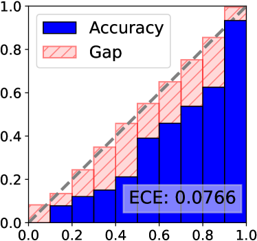
Confidence Calibration. We further study the model calibration of GMMSeg and the discriminative counterpart, i.e., DeepLab${}_{\text{V3+}}$ [49] with the softmax classifier. In Fig. 5, we illustrate the Expected Calibration Error (ECE) [15] along with reliability diagrams, which plot the expected pixel accuracy as a function of confidence [15]. As seen, GMMSeg yields better calibrated prefictions, i.e., smaller gaps between the expected accuracy and confidence. On the other hand, the discriminative softmax produces confidences that deviate more from the true probabilities, and suffers higher calibration error accordingly, which again verifies the better reliability and interpretability of GMMSeg compared to its discriminative counterparts.

Runtime Analysis. The inference speed of GMMSeg is $13.37$ fps, which only yields negligible overhead w.r.t. its discriminative softmax counterpart, i.e., $13.37$ vs. $14.16$ fps. We measure the fps with a single NVIDIA GeForce RTX 3090 GPU with a batch size of one.

5 Conclusion

We${}_{\!}$ presented${}_{\!}$ GMMSeg,${}_{\!}$ the${}_{\!}$ first${}_{\!}$ generative${}_{\!}$ neural${}_{\!}$ framework${}_{\!}$ for${}_{\!}$ semantic${}_{\!}$ segmentation.${}_{\!}$ By${}_{\!}$ explicitly${}_{\!}$ modeling data distribution as GMMs, GMMSeg shows promise to solve the intrinsic limitations of current softmax based discriminative regime. It successfully optimizes generative GMM with end-to-end discriminative representation learning in a compact and collaborative manner. This makes GMMSeg principled and well applicable in both closed-set and open-world settings. We believe this
work provides fundamental insights and can benefit a broad range of application tasks. As a part of our${}_{\!}$ future${}_{\!}$ work,${}_{\!}$ we${}_{\!}$ will${}_{\!}$ explore${}_{\!}$ our${}_{\!}$ algorithm${}_{\!}$ in${}_{\!}$ image${}_{\!}$ classification${}_{\!}$ and${}_{\!}$ trustworthy${}_{\!}$ AI${}_{\!}$ related${}_{\!}$ tasks.

SUMMARY OF THE APPENDIX

In the appendix, we provide the following items that shed deeper insight on our contributions:

• §A: Detailed training parameters.

• §B: More experimental results.

• §C: More qualitative visualization.

Appendix A Detailed Training Parameters

We evaluate our GMMSeg on six base segmentation architectures. Four of them, i.e., DeepLab${}_{\text{v3+}}$ [47], OCRNet[48], Swin-UperNet [52], SegFormer [7], are presented in our main paper. And the two additional base architectures, i.e., FCN [1] and Mask2Former [90], are provided in this supplemental material (cf. §B). We follow the default training settings in the official Mask2Former codebase and MMSegmentation for Mask2Former and other base architectures respectively. In particular, we train FCN, DeepLab${}_{\text{v3+}}$ and OCRNet using SGD optimizer with initial learning rate $0.1$, weight decay 4e-4 with polynomial learning rate annealing; we train Swin-UperNet and SegFormer using AdamW optimizer with initial learning rate 6e-5, weight decay 1e-2 with polynomial learning rate annealing; we train Mask2Former using AdamW optimizer with initial learning rate 1e-4, weight decay 5e-2 and the learning rate is decayed by a factor of 10 at 0.9 and 0.95 fractions of the total training steps.

Appendix B More Experimental Results

More Base Segmentation Architectures. We first demonstrate the efficacy of our GMMSeg on two additional base segmentation architectures, i.e., FCN [1] and Mask2Former [90], with quantitative results summarized in Table B. We train FCN based models with the according training hyperparameter

Table 6: Additional quantitative results (§B) on ADE${}_{\text{20K}\!}$ [53] val, Cityscapes${}_{\!}$ [54] val, and COCO-Stuff${}_{\!}$ [55] test in mean IoU.

Method					Backbone	ADE${}_{\text{20K}}$	Citys.	​​​COCO.​​​
FCN [CVPR15] [1]		39.9	75.5	32.6
GMMSeg	ResNet${}_{\text{101}}$	41.8 $\!\uparrow\!$ 1.9	76.7 $\!\uparrow\!$ 1.2	34.1 $\!\uparrow\!$ 1.5
Mask2Former [CVPR22] [90]		56.1	83.3	51.0
GMMSeg	Swin${}_{\text{Large}}$	56.7 $\!\uparrow\!$ 0.6	83.8 $\!\uparrow\!$ 0.5	52.0 $\!\uparrow\!$ 1.0
1-5[1pt/1pt]

settings mentioned in §A and strictly follow the same training and inference setups in our main manuscript (cf. §4.1). Furthermore, for a fair comparison with Mask2Former, the backbone, i.e., Swin${}_{\text{Large}}$ [52], is pretrained with ImageNet${}_{\text{22K}}$ [123]. For ADE${}_{\text{20K}}$/COCO-Stuff/Cityscapes, we train Mask2Former based models using images cropped to $640\!\times\!640$/$640\!\times\!640$/$1024\!\times\!1024$, for $160$K/$80$K/$90$K iterations with $16$/$16$/$16$ batch size. We adopt sliding window inference on Cityscapes with a window size of $1024\!\times\!1024$ and we keep the aspect ratio of test images and rescale the short side to $640$ on ADE${}_{\text{20K}}$ and COCO-Stuff.

Here FCN is a famous fully convolutional model that is in line with the per-pixel dense classification models we discussed in the main paper (cf. §3.1). Besides, of particular interest is the Mask2Former, which is an attentive model proposed very recently that formulates the task as a mask classification problem, where a mask-level representation is learned instead of pixel-level. However, it still relies on a discriminative softmax based classifier for mask classification. We equip Mask2Former by replacing the softmax classification module with our generative GMM classifier.

As seen, GMMSeg consistently boosts the model performance despite different segmentation formulations, i.e., pixel classification or mask classification, verifying the superiority of our GMMSeg that brings a paradigm shift from a discriminative softmax to a generative GMM. Notably, with Mask2Former-Swin${}_{\text{Large}}$ as base segmentation architecture, our GMMSeg earns mIoU scores of 56.7%/83.8%/52.0%, establishing new state-of-the-arts among ADE${}_{\text{20K}}$/Cityscapes/COCO-Stuff.

Anomaly Segmentation Result on Fishyscapes Lost&Found test and Static test. We additionally report the anomaly segmentation performance of our Cityscapes [54] trained GMMSeg built upon DeepLab${}_{\text{V3+}}$ [47]-ResNet${}_{\text{101}}$ [50] on Fishyscapes [56] Lost&Found test and Static test. Fishyscapes Static is a blending-based dataset built upon backgrounds from Cityscapes and anomalous objects from Pascal VOC [126], that contains $30$/$1,000$ images in val/test set. The test splits of Fishyscapes Lost&Found and Static are privately held by the Fishyscapes organization that contain entirely unknown anomalies to the methods. The results are summarized in Table 7, and are also publicly available in anonymous on the official leaderboard. We categorize the methods by checking whether they require retraining, extra segmentation networks or utilize OoD data, following [56, 18].

As seen, without any add-on post-calibration technique, GMMSeg significantly surpasses the state-of-the-art methods by even larger margins on the challenging test set compared to results on val set, i.e., +24.58%/+14.91% in AP and +22.91%/+3.68% in FPR${}_{\text{95}}$ on Fishyscapes Lost&Found/Static test. Notably, GMMSeg even outperforms all other benchmark methods that employ additional training networks/data on Fishyscapes Lost&Found test, verifying the strong robustness to unexpected anomalies on-road due to the accurate data density modeling of GMMSeg.

Table 7: Quantitative results (§B) on Fishyscapes (FS) Lost&Found test and Static test.

	Re-	Extra	OoD	FS Lost&Found		FS Static
Method	training	Network	Data	AP $\uparrow$	FPR${}_{\text{95}}$ $\downarrow$	AP $\uparrow$	FPR${}_{\text{95}}$ $\downarrow$
Density - Single-layer NLL [56]	✗	✓	✗	3.01	32.9	40.86	21.29
Density - Minimum NLL [56]	✗	✓	✗	4.25	47.15	62.14	17.43
Density - Logistic Regression [56]	✗	✓	✓	4.65	24.36	57.16	13.39
Image Resynthesis [36]	✗	✓	✗	5.70	48.05	29.6	27.13
Bayesian Deeplab [46]	✓	✗	✗	9.81	38.46	48.70	15.05
OoD Training - Void Class [127]	✓	✗	✓	10.29	22.11	45.00	19.40
Discriminative Outlier Detection Head [38]	✓	✓	✓	31.31	19.02	96.76	0.29
Dirichlet Deeplab [128]	✓	✗	✓	34.28	47.43	31.30	84.60
SynBoost [34]	✗	✓	✓	43.22	15.79	72.59	18.75
MSP [129]	✗	✗	✗	1.77	44.85	12.88	39.83
Entropy [17]	✗	✗	✗	2.93	44.83	15.41	39.75
kNN Embedding - density [56]	✗	✗	✗	3.55	30.02	44.03	20.25
SML [18]	✗	✗	✗	31.05	21.52	53.11	19.64
GMMSeg-DeepLab${}_{\text{V3+}}$	✗	✗	✗	55.63	6.61	76.02	15.96

Table 8: Impact of memory size, evaluated on ADE${}_{\text{20K}\!}$ [53] val.

# Sample	mIoU (%)
0	40.3
8K	45.1
16K	45.4
32K	46.0
48K	46.0

Impact of Memory Capacity. In Table 8, we further explore the influence of the memory capacity, i.e., the amount of pixel representations stored for class-wise EM estimation, with DeepLab${}_{\text{V3+}}$-ResNet${}_{\text{101}}$ on ADE${}_{\text{20K}}$ val trained for 80K iterations. For the first row, where the memory size is set to $0$, the EM is only performed within mini-batches. Not surprisingly, data distribution estimated at such a local scale is far from accurate, leading to inferior results. With enlarged memory capacity, the performance is increased. When the performance reaches saturation, the stored pixel samples are sufficient enough to represent the true data distribution of the whole training set.

Appendix C More Qualitative Visualization

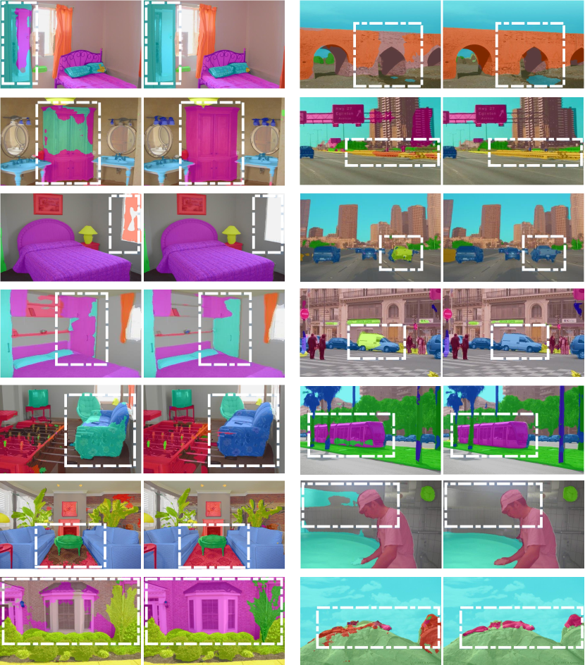
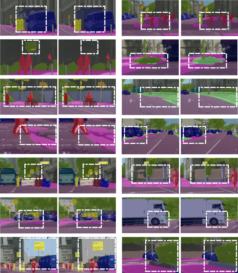
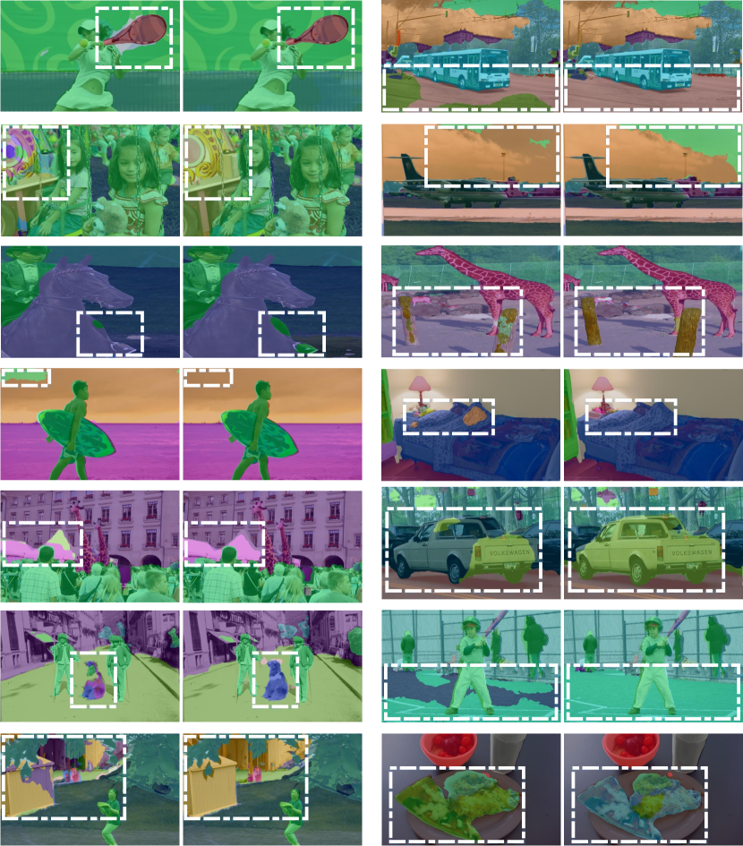
Semantic${}_{\!}$ Segmentation. We${}_{\!}$ illustrate${}_{\!}$ the${}_{\!}$ qualitative${}_{\!}$ comparisons${}_{\!}$ of${}_{\!}$ GMMSeg${}_{\!}$ equipped${}_{\!}$ SegFormer [7]-MiT${}_{\text{B5}}$${}_{\!}$ against${}_{\!}$ the${}_{\!}$ original${}_{\!}$ model${}_{\!}$ on${}_{\!}$ ADE${}_{\text{20K}}$${}_{\!}$ [53]${}_{\!}$ (Fig.${}_{\!}$ 6),${}_{\!}$ Cityscapes${}_{\!}$ [54]${}_{\!}$ (Fig.${}_{\!}$ 7)${}_{\!}$ and${}_{\!}$ COCO-Stuff${}_{\!}$ [55]${}_{\!}$ (Fig.${}_{\!}$ 8). It is evident that, benefiting from the accurate data characterization modeling, GMMSeg is less confused by object categories and gives preciser predictions than SegFormer.

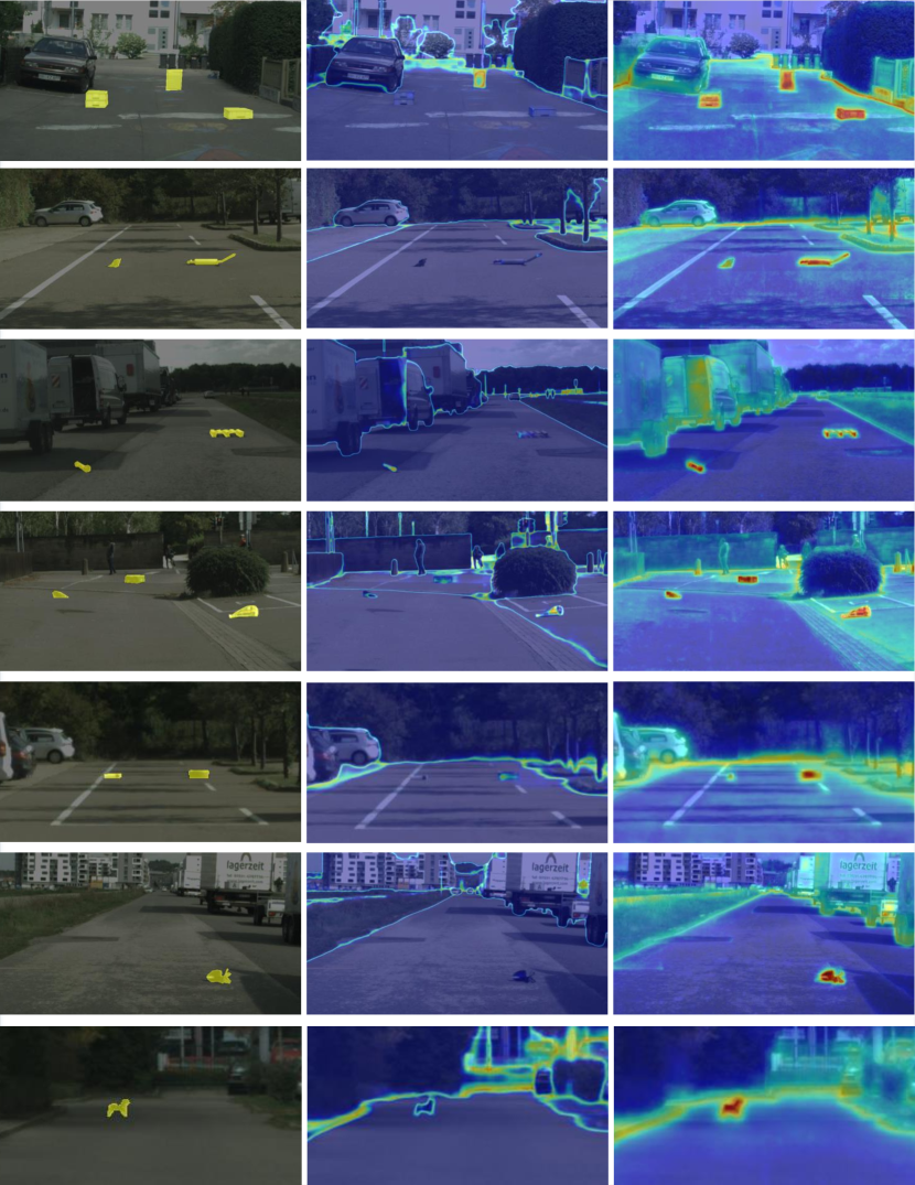
Anomaly${}_{\!}$ Segmentation. We${}_{\!}$ then${}_{\!}$ show${}_{\!}$ more${}_{\!}$ qualitative${}_{\!}$ results${}_{\!}$ of${}_{\!}$ MSP [17]-DeepLab${}_{\text{V3+}}$ [47]${}_{\!}$ and${}_{\!}$ GMMSeg-DeepLab${}_{\text{V3+}}$${}_{\!}$ on${}_{\!}$ Fishyscapes${}_{\!}$ Lost&Found${}_{\!}$ val. As observed, different from MSP, GMMSeg gets rid of being overwhelmed by overconfident predictions and successfully identifies the anomalies.

Figure 6: Qualitative results (§C) of SegFormer [7] and our GMMSeg on ADE${}_{\text{20K}}$ [53].

Figure 7: Qualitative results (§C) of SegFormer [7] and our GMMSeg on Cityscapes [54].

Figure 8: Qualitative results (§C) of SegFormer [7] and our GMMSeg on COCO-Stuff [55].

Figure 9: Qualitative results (§C) of anomaly heatmaps on Fishyscapes Lost&Found [56] val.

References

- [1] Jonathan Long, Evan Shelhamer, and Trevor Darrell. Fully convolutional networks for semantic segmentation. In CVPR, 2015.
- [2] Liang-Chieh Chen, George Papandreou, Iasonas Kokkinos, Kevin Murphy, and Alan L Yuille. Deeplab: Semantic image segmentation with deep convolutional nets, atrous convolution, and fully connected crfs. IEEE TPAMI, 2017.
- [3] Hengshuang Zhao, Jianping Shi, Xiaojuan Qi, Xiaogang Wang, and Jiaya Jia. Pyramid scene parsing network. In CVPR, 2017.
- [4] Jie Hu, Li Shen, and Gang Sun. Squeeze-and-excitation networks. In CVPR, 2018.
- [5] Jun Fu, Jing Liu, Haijie Tian, Yong Li, Yongjun Bao, Zhiwei Fang, and Hanqing Lu. Dual attention network for scene segmentation. In CVPR, 2019.
- [6] Ashish Vaswani, Noam Shazeer, Niki Parmar, Jakob Uszkoreit, Llion Jones, Aidan N Gomez, Lukasz Kaiser, and Illia Polosukhin. Attention is all you need. In NeurIPS, 2017.
- [7] Enze Xie, Wenhai Wang, Zhiding Yu, Anima Anandkumar, Jose M Alvarez, and Ping Luo. Segformer: Simple and efficient design for semantic segmentation with transformers. In NeurIPS, 2021.
- [8] Robin Strudel, Ricardo Garcia, Ivan Laptev, and Cordelia Schmid. Segmenter: Transformer for semantic segmentation. In ICCV, 2021.
- [9] Sixiao Zheng, Jiachen Lu, Hengshuang Zhao, Xiatian Zhu, Zekun Luo, Yabiao Wang, Yanwei Fu, Jianfeng Feng, Tao Xiang, Philip HS Torr, et al. Rethinking semantic segmentation from a sequence-to-sequence perspective with transformers. In CVPR, 2021.
- [10] Yuhui Yuan, Rao Fu, Lang Huang, Weihong Lin, Chao Zhang, Xilin Chen, and Jingdong Wang. Hrformer: High-resolution transformer for dense prediction. In NeurIPS, 2021.
- [11] JM Bernardo, MJ Bayarri, JO Berger, AP Dawid, D Heckerman, AFM Smith, and M West. Generative or discriminative? getting the best of both worlds. Bayesian statistics, 8(3):3–24, 2007.
- [12] Hideaki Hayashi and Seiichi Uchida. A discriminative gaussian mixture model with sparsity. In ICLR, 2021.
- [13] Tianfei Zhou, Wenguan Wang, Ender Konukoglu, and Luc Van Gool. Rethinking semantic segmentation: A prototype view. In CVPR, 2022.
- [14] Lynton Ardizzone, Radek Mackowiak, Carsten Rother, and Ullrich Köthe. Training normalizing flows with the information bottleneck for competitive generative classification. In NeurIPS, 2020.
- [15] Chuan Guo, Geoff Pleiss, Yu Sun, and Kilian Q Weinberger. On calibration of modern neural networks. In ICML, 2017.
- [16] Yaniv Ovadia, Emily Fertig, Jie Ren, Zachary Nado, David Sculley, Sebastian Nowozin, Joshua Dillon, Balaji Lakshminarayanan, and Jasper Snoek. Can you trust your model’s uncertainty? evaluating predictive uncertainty under dataset shift. NeurIPS, 2019.
- [17] Dan Hendrycks and Kevin Gimpel. A baseline for detecting misclassified and out-of-distribution examples in neural networks. In ICLR, 2017.
- [18] Sanghun Jung, Jungsoo Lee, Daehoon Gwak, Sungha Choi, and Jaegul Choo. Standardized max logits: A simple yet effective approach for identifying unexpected road obstacles in urban-scene segmentation. In ICCV, 2021.
- [19] Kimin Lee, Kibok Lee, Honglak Lee, and Jinwoo Shin. A simple unified framework for detecting out-of-distribution samples and adversarial attacks. NeurIPS, 2018.
- [20] Bradley Efron. The efficiency of logistic regression compared to normal discriminant analysis. Journal of the American Statistical Association, 70(352):892–898, 1975.
- [21] Andrew Ng and Michael Jordan. On discriminative vs. generative classifiers: A comparison of logistic regression and naive bayes. In NeurIPS, 2001.
- [22] Eric Nalisnick, Akihiro Matsukawa, Yee Whye Teh, Dilan Gorur, and Balaji Lakshminarayanan. Hybrid models with deep and invertible features. In ICML, 2019.
- [23] Pavel Izmailov, Polina Kirichenko, Marc Finzi, and Andrew Gordon Wilson. Semi-supervised learning with normalizing flows. In ICML, 2020.
- [24] Radek Mackowiak, Lynton Ardizzone, Ullrich Kothe, and Carsten Rother. Generative classifiers as a basis for trustworthy image classification. In CVPR, 2021.
- [25] Lukas Schott, Jonas Rauber, Matthias Bethge, and Wieland Brendel. Towards the first adversarially robust neural network model on mnist. In NeurIPS, 2018.
- [26] Yang Song, Taesup Kim, Sebastian Nowozin, Stefano Ermon, and Nate Kushman. Pixeldefend: Leveraging generative models to understand and defend against adversarial examples. In ICLR, 2018.
- [27] Joan Serrà, David Álvarez, Vicenç Gómez, Olga Slizovskaia, José F Núñez, and Jordi Luque. Input complexity and out-of-distribution detection with likelihood-based generative models. In ICLR, 2019.
- [28] Gonzalo Mena, Amin Nejatbakhsh, Erdem Varol, and Jonathan Niles-Weed. Sinkhorn em: an expectation-maximization algorithm based on entropic optimal transport. arXiv preprint arXiv:2006.16548, 2020.
- [29] Ehsan Variani, Erik McDermott, and Georg Heigold. A gaussian mixture model layer jointly optimized with discriminative features within a deep neural network architecture. In ICASSP, 2015.
- [30] Zoltán Tüske, Muhammad Ali Tahir, Ralf Schlüter, and Hermann Ney. Integrating gaussian mixtures into deep neural networks: Softmax layer with hidden variables. In ICASSP, 2015.
- [31] Aldebaro Klautau, Nikola Jevtic, and Alon Orlitsky. Discriminative gaussian mixture models: A comparison with kernel classifiers. In ICML, 2003.
- [32] Zhihao Zheng and Pengyu Hong. Robust detection of adversarial attacks by modeling the intrinsic properties of deep neural networks. In NeurIPS, 2018.
- [33] Kimin Lee, Sukmin Yun, Kibok Lee, Honglak Lee, Bo Li, and Jinwoo Shin. Robust inference via generative classifiers for handling noisy labels. In ICML, 2019.
- [34] Giancarlo Di Biase, Hermann Blum, Roland Siegwart, and Cesar Cadena. Pixel-wise anomaly detection in complex driving scenes. In CVPR, 2021.
- [35] Yingda Xia, Yi Zhang, Fengze Liu, Wei Shen, and Alan L Yuille. Synthesize then compare: Detecting failures and anomalies for semantic segmentation. In ECCV, 2020.
- [36] Krzysztof Lis, Krishna Nakka, Pascal Fua, and Mathieu Salzmann. Detecting the unexpected via image resynthesis. In ICCV, 2019.
- [37] Tomas Vojir, Tomáš Šipka, Rahaf Aljundi, Nikolay Chumerin, Daniel Olmeda Reino, and Jiri Matas. Road anomaly detection by partial image reconstruction with segmentation coupling. In ICCV, 2021.
- [38] Petra Bevandić, Ivan Krešo, Marin Oršić, and Siniša Šegvić. Simultaneous semantic segmentation and outlier detection in presence of domain shift. In GCPR, 2019.
- [39] Robin Chan, Matthias Rottmann, and Hanno Gottschalk. Entropy maximization and meta classification for out-of-distribution detection in semantic segmentation. In ICCV, 2021.
- [40] Dan Hendrycks, Mantas Mazeika, and Thomas Dietterich. Deep anomaly detection with outlier exposure. arXiv preprint arXiv:1812.04606, 2018.
- [41] Shiyu Liang, Yixuan Li, and Rayadurgam Srikant. Enhancing the reliability of out-of-distribution image detection in neural networks. arXiv preprint arXiv:1706.02690, 2017.
- [42] KIMIN LEE, Kibok Lee, Honglak Lee, and Jinwoo Shin. Training confidence-calibrated classifiers for detecting out-of-distribution samples. In ICLR, 2018.
- [43] Matthias Rottmann, Pascal Colling, Thomas Paul Hack, Robin Chan, Fabian Hüger, Peter Schlicht, and Hanno Gottschalk. Prediction error meta classification in semantic segmentation: Detection via aggregated dispersion measures of softmax probabilities. In IJCNN, 2020.
- [44] Alex Kendall and Yarin Gal. What uncertainties do we need in bayesian deep learning for computer vision? In Advances in neural information processing systems, 2017.
- [45] Balaji Lakshminarayanan, Alexander Pritzel, and Charles Blundell. Simple and scalable predictive uncertainty estimation using deep ensembles. In NeurIPS, 2017.
- [46] Jishnu Mukhoti and Yarin Gal. Evaluating bayesian deep learning methods for semantic segmentation. arXiv preprint arXiv:1811.12709, 2018.
- [47] Liang-Chieh Chen, Yukun Zhu, George Papandreou, Florian Schroff, and Hartwig Adam. Encoder-decoder with atrous separable convolution for semantic image segmentation. In ECCV, 2018.
- [48] Yuhui Yuan, Xilin Chen, and Jingdong Wang. Object-contextual representations for semantic segmentation. In ECCV, 2020.
- [49] Tete Xiao, Yingcheng Liu, Bolei Zhou, Yuning Jiang, and Jian Sun. Unified perceptual parsing for scene understanding. In ECCV, 2018.
- [50] Kaiming He, Xiangyu Zhang, Shaoqing Ren, and Jian Sun. Deep residual learning for image recognition. In CVPR, 2016.
- [51] Jingdong Wang, Ke Sun, Tianheng Cheng, Borui Jiang, Chaorui Deng, Yang Zhao, Dong Liu, Yadong Mu, Mingkui Tan, Xinggang Wang, et al. Deep high-resolution representation learning for visual recognition. IEEE TPAMI, 2020.
- [52] Ze Liu, Yutong Lin, Yue Cao, Han Hu, Yixuan Wei, Zheng Zhang, Stephen Lin, and Baining Guo. Swin transformer: Hierarchical vision transformer using shifted windows. In ICCV, 2021.
- [53] Bolei Zhou, Hang Zhao, Xavier Puig, Sanja Fidler, Adela Barriuso, and Antonio Torralba. Scene parsing through ade20k dataset. In CVPR, 2017.
- [54] Marius Cordts, Mohamed Omran, Sebastian Ramos, Timo Rehfeld, Markus Enzweiler, Rodrigo Benenson, Uwe Franke, Stefan Roth, and Bernt Schiele. The cityscapes dataset for semantic urban scene understanding. In CVPR, 2016.
- [55] Holger Caesar, Jasper Uijlings, and Vittorio Ferrari. Coco-stuff: Thing and stuff classes in context. In CVPR, 2018.
- [56] Hermann Blum, Paul-Edouard Sarlin, Juan Nieto, Roland Siegwart, and Cesar Cadena. The fishyscapes benchmark: Measuring blind spots in semantic segmentation. IJCV, 2021.
- [57] Jifeng Dai, Haozhi Qi, Yuwen Xiong, Yi Li, Guodong Zhang, Han Hu, and Yichen Wei. Deformable convolutional networks. In CVPR, 2017.
- [58] Maoke Yang, Kun Yu, Chi Zhang, Zhiwei Li, and Kuiyuan Yang. Denseaspp for semantic segmentation in street scenes. In CVPR, 2018.
- [59] Fisher Yu and Vladlen Koltun. Multi-scale context aggregation by dilated convolutions. In ICLR, 2016.
- [60] Guolei Sun, Wenguan Wang, Jifeng Dai, and Luc Van Gool. Mining cross-image semantics for weakly supervised semantic segmentation. In ECCV, 2020.
- [61] Olaf Ronneberger, Philipp Fischer, and Thomas Brox. U-net: Convolutional networks for biomedical image segmentation. In MICCAI, 2015.
- [62] Shuai Zheng, Sadeep Jayasumana, Bernardino Romera-Paredes, Vibhav Vineet, Zhizhong Su, Dalong Du, Chang Huang, and Philip HS Torr. Conditional random fields as recurrent neural networks. In ICCV, 2015.
- [63] Vijay Badrinarayanan, Alex Kendall, and Roberto Cipolla. Segnet: A deep convolutional encoder-decoder architecture for image segmentation. IEEE TPAMI, 39(12):2481–2495, 2017.
- [64] Ziwei Liu, Xiaoxiao Li, Ping Luo, Chen Change Loy, and Xiaoou Tang. Deep learning markov random field for semantic segmentation. IEEE TPAMI, 40(8):1814–1828, 2017.
- [65] Guosheng Lin, Anton Milan, Chunhua Shen, and Ian Reid. Refinenet: Multi-path refinement networks for high-resolution semantic segmentation. In CVPR, 2017.
- [66] Sachin Mehta, Mohammad Rastegari, Anat Caspi, Linda Shapiro, and Hannaneh Hajishirzi. Espnet: Efficient spatial pyramid of dilated convolutions for semantic segmentation. In ECCV, 2018.
- [67] Hang Zhang, Kristin Dana, Jianping Shi, Zhongyue Zhang, Xiaogang Wang, Ambrish Tyagi, and Amit Agrawal. Context encoding for semantic segmentation. In CVPR, 2018.
- [68] Junjun He, Zhongying Deng, Lei Zhou, Yali Wang, and Yu Qiao. Adaptive pyramid context network for semantic segmentation. In CVPR, 2019.
- [69] Hanzhe Hu, Deyi Ji, Weihao Gan, Shuai Bai, Wei Wu, and Junjie Yan. Class-wise dynamic graph convolution for semantic segmentation. In ECCV, 2020.
- [70] Changqian Yu, Jingbo Wang, Changxin Gao, Gang Yu, Chunhua Shen, and Nong Sang. Context prior for scene segmentation. In CVPR, 2020.
- [71] Mingyuan Liu, Dan Schonfeld, and Wei Tang. Exploit visual dependency relations for semantic segmentation. In CVPR, 2021.
- [72] Chi-Wei Hsiao, Cheng Sun, Hwann-Tzong Chen, and Min Sun. Specialize and fuse: Pyramidal output representation for semantic segmentation. In ICCV, 2021.
- [73] Zhenchao Jin, Bin Liu, Qi Chu, and Nenghai Yu. Isnet: Integrate image-level and semantic-level context for semantic segmentation. In ICCV, 2021.
- [74] Zhenchao Jin, Tao Gong, Dongdong Yu, Qi Chu, Jian Wang, Changhu Wang, and Jie Shao. Mining contextual information beyond image for semantic segmentation. In ICCV, 2021.
- [75] Wenguan Wang, Tianfei Zhou, Fisher Yu, Jifeng Dai, Ender Konukoglu, and Luc Van Gool. Exploring cross-image pixel contrast for semantic segmentation. In ICCV, 2021.
- [76] Jiaxu Miao, Yunchao Wei, Yu Wu, Chen Liang, Guangrui Li, and Yi Yang. Vspw: A large-scale dataset for video scene parsing in the wild. In CVPR, 2021.
- [77] Zongxin Yang, Yunchao Wei, and Yi Yang. Collaborative video object segmentation by multi-scale foreground-background integration. IEEE TPAMI, 2021.
- [78] Adam W Harley, Konstantinos G Derpanis, and Iasonas Kokkinos. Segmentation-aware convolutional networks using local attention masks. In ICCV, 2017.
- [79] Xiaolong Wang, Ross Girshick, Abhinav Gupta, and Kaiming He. Non-local neural networks. In CVPR, 2018.
- [80] Hanchao Li, Pengfei Xiong, Jie An, and Lingxue Wang. Pyramid attention network for semantic segmentation. arXiv preprint arXiv:1805.10180, 2018.
- [81] Hengshuang Zhao, Yi Zhang, Shu Liu, Jianping Shi, Chen Change Loy, Dahua Lin, and Jiaya Jia. Psanet: Point-wise spatial attention network for scene parsing. In ECCV, 2018.
- [82] Junjun He, Zhongying Deng, and Yu Qiao. Dynamic multi-scale filters for semantic segmentation. In ICCV, 2019.
- [83] Xia Li, Zhisheng Zhong, Jianlong Wu, Yibo Yang, Zhouchen Lin, and Hong Liu. Expectation-maximization attention networks for semantic segmentation. In ICCV, 2019.
- [84] Zilong Huang, Xinggang Wang, Lichao Huang, Chang Huang, Yunchao Wei, and Wenyu Liu. Ccnet: Criss-cross attention for semantic segmentation. In ICCV, 2019.
- [85] Liulei Li, Tianfei Zhou, Wenguan Wang, Jianwu Li, and Yi Yang. Deep hierarchical semantic segmentation. In CVPR, pages 1246–1257, 2022.
- [86] Wenguan Wang, Hailong Zhu, Jifeng Dai, Yanwei Pang, Jianbing Shen, and Ling Shao. Hierarchical human parsing with typed part-relation reasoning. In CVPR, 2020.
- [87] Wenguan Wang, Zhijie Zhang, Siyuan Qi, Jianbing Shen, Yanwei Pang, and Ling Shao. Learning compositional neural information fusion for human parsing. In ICCV, 2019.
- [88] Zongxin Yang, Yunchao Wei, and Yi Yang. Associating objects with transformers for video object segmentation. NeurIPS, 2021.
- [89] Bowen Cheng, Alexander G. Schwing, and Alexander Kirillov. Per-pixel classification is not all you need for semantic segmentation. In NeurIPS, 2021.
- [90] Bowen Cheng, Ishan Misra, Alexander G Schwing, Alexander Kirillov, and Rohit Girdhar. Masked-attention mask transformer for universal image segmentation. CVPR, 2022.
- [91] Weiyang Liu, Yandong Wen, Zhiding Yu, and Meng Yang. Large-margin softmax loss for convolutional neural networks. In ICML, 2016.
- [92] Yi Yang, Yueting Zhuang, and Yunhe Pan. Multiple knowledge representation for big data artificial intelligence: framework, applications, and case studies. Frontiers of Information Technology & Electronic Engineering, 22(12):1551–1558, 2021.
- [93] Wenguan Wang, Cheng Han, Tianfei Zhou, and Dongfang Liu. Visual recognition with deep nearest centroids. arXiv preprint arXiv:2209.07383, 2022.
- [94] Jyh-Jing Hwang, Stella X Yu, Jianbo Shi, Maxwell D Collins, Tien-Ju Yang, Xiao Zhang, and Liang-Chieh Chen. Segsort: Segmentation by discriminative sorting of segments. In ICCV, 2019.
- [95] Arindam Banerjee, Inderjit S Dhillon, Joydeep Ghosh, Suvrit Sra, and Greg Ridgeway. Clustering on the unit hypersphere using von mises-fisher distributions. Journal of Machine Learning Research, 6(9), 2005.
- [96] Rajat Raina, Yirong Shen, Andrew Mccallum, and Andrew Ng. Classification with hybrid generative/discriminative models. NeurIPS, 2003.
- [97] Tim Salimans, Ian Goodfellow, Wojciech Zaremba, Vicki Cheung, Alec Radford, and Xi Chen. Improved techniques for training gans. In NeurIPS, 2016.
- [98] Ricky TQ Chen, Jens Behrmann, David K Duvenaud, and Jörn-Henrik Jacobsen. Residual flows for invertible generative modeling. In NeurIPS, 2019.
- [99] Will Grathwohl, Kuan-Chieh Wang, Joern-Henrik Jacobsen, David Duvenaud, Mohammad Norouzi, and Kevin Swersky. Your classifier is secretly an energy based model and you should treat it like one. In ICLR, 2019.
- [100] Yingzhen Li, John Bradshaw, and Yash Sharma. Are generative classifiers more robust to adversarial attacks? In ICML, 2019.
- [101] Xinshuai Dong, Hong Liu, Rongrong Ji, Liujuan Cao, Qixiang Ye, Jianzhuang Liu, and Qi Tian. Api-net: Robust generative classifier via a single discriminator. In ECCV, 2020.
- [102] Ethan Fetaya, Jörn-Henrik Jacobsen, Will Grathwohl, and Richard Zemel. Understanding the limitations of conditional generative models. 2020.
- [103] Eric Nalisnick, Akihiro Matsukawa, Yee Whye Teh, Dilan Gorur, and Balaji Lakshminarayanan. Do deep generative models know what they don’t know? In ICLR, 2019.
- [104] Florian Wenzel, Théo Galy-Fajou, Christan Donner, Marius Kloft, and Manfred Opper. Efficient gaussian process classification using pòlya-gamma data augmentation. In AAAI, 2019.
- [105] Tommi Jaakkola and David Haussler. Exploiting generative models in discriminative classifiers. In NeurIPS, 1998.
- [106] Julia A Lasserre, Christopher M Bishop, and Thomas P Minka. Principled hybrids of generative and discriminative models. In CVPR, 2006.
- [107] Hyunsun Choi, Eric Jang, and Alexander A Alemi. Waic, but why? generative ensembles for robust anomaly detection. arXiv preprint arXiv:1810.01392, 2018.
- [108] Jie Ren, Peter J Liu, Emily Fertig, Jasper Snoek, Ryan Poplin, Mark Depristo, Joshua Dillon, and Balaji Lakshminarayanan. Likelihood ratios for out-of-distribution detection. In NeurIPS, 2019.
- [109] Durk P Kingma, Shakir Mohamed, Danilo Jimenez Rezende, and Max Welling. Semi-supervised learning with deep generative models. In NeurIPS, 2014.
- [110] Guillaume Bouchard and Bill Triggs. The tradeoff between generative and discriminative classifiers. In IASC International Symposium on Computational Statistics, 2004.
- [111] Thomas Mensink, Jakob Verbeek, Florent Perronnin, and Gabriela Csurka. Distance-based image classification: Generalizing to new classes at near-zero cost. IEEE TPAMI, 35(11):2624–2637, 2013.
- [112] Kateryna Chumachenko, Alexandros Iosifidis, and Moncef Gabbouj. Feedforward neural networks initialization based on discriminant learning. Neural Networks, 146:220–229, 2022.
- [113] Murat Sensoy, Lance Kaplan, and Melih Kandemir. Evidential deep learning to quantify classification uncertainty. In NeurIPS, 2020.
- [114] Arthur P Dempster, Nan M Laird, and Donald B Rubin. Maximum likelihood from incomplete data via the em algorithm. Journal of the Royal Statistical Society: Series B (Methodological), 39(1):1–22, 1977.
- [115] Radford M Neal and Geoffrey E Hinton. A view of the em algorithm that justifies incremental, sparse, and other variants. In Learning in graphical models, pages 355–368. 1998.
- [116] Naonori Ueda and Ryohei Nakano. Deterministic annealing variant of the em algorithm. NeurIPS, 7, 1994.
- [117] Yuki Markus Asano, Christian Rupprecht, and Andrea Vedaldi. Self-labelling via simultaneous clustering and representation learning. In ICLR, 2020.
- [118] Marco Cuturi. Sinkhorn distances: Lightspeed computation of optimal transport. In NeurIPS, 2013.
- [119] Steven Nowlan. Maximum likelihood competitive learning. NeurIPS, 1989.
- [120] Nanda Kambhatla and Todd Leen. Classifying with gaussian mixtures and clusters. NeurIPS, 1994.
- [121] Xuefeng Du, Xin Wang, Gabriel Gozum, and Yixuan Li. Unknown-aware object detection: Learning what you don’t know from videos in the wild. In CVPR, 2022.
- [122] MMSegmentation Contributors. MMSegmentation: Openmmlab semantic segmentation toolbox and benchmark. https://github.com/open-mmlab/mmsegmentation, 2020.
- [123] Olga Russakovsky, Jia Deng, Hao Su, Jonathan Krause, Sanjeev Satheesh, Sean Ma, Zhiheng Huang, Andrej Karpathy, Aditya Khosla, Michael S. Bernstein, Alexander C. Berg, and Fei-Fei Li. Imagenet large scale visual recognition challenge. IJCV, 115(3):211–252, 2015.
- [124] Peter Pinggera, Sebastian Ramos, Stefan Gehrig, Uwe Franke, Carsten Rother, and Rudolf Mester. Lost and found: detecting small road hazards for self-driving vehicles. In IROS, 2016.
- [125] Weitang Liu, Xiaoyun Wang, John Owens, and Yixuan Li. Energy-based out-of-distribution detection. NeurIPS, 2020.
- [126] Mark Everingham, SM Eslami, Luc Van Gool, Christopher KI Williams, John Winn, and Andrew Zisserman. The pascal visual object classes challenge: A retrospective. IJCV, 2015.
- [127] Terrance DeVries and Graham W Taylor. Learning confidence for out-of-distribution detection in neural networks. arXiv preprint arXiv:1802.04865, 2018.
- [128] Andrey Malinin and Mark Gales. Predictive uncertainty estimation via prior networks. NeurIPS, 2018.
- [129] Dan Hendrycks, Steven Basart, Mantas Mazeika, Mohammadreza Mostajabi, Jacob Steinhardt, and Dawn Song. Scaling out-of-distribution detection for real-world settings. arXiv preprint arXiv:1911.11132, 2019.