Opportunistic Qualitative Planning in Stochastic Systems with Incomplete Preferences over Reachability Objectives

Abstract

Preferences play a key role in determining what goals/constraints to satisfy when not all constraints can be satisfied simultaneously. In this paper, we study how to synthesize preference satisfying plans in stochastic systems, modeled as a Markov Decision Process (MDP), given a (possibly incomplete) combinative preference model over temporally extended goals. We start by introducing new semantics to interpret preferences over infinite plays of the stochastic system. Then, we introduce a new notion of improvement to enable comparison between two prefixes of an infinite play. Based on this, we define two solution concepts called Safe and Positive Improving (SPI) and Safe and Almost-Sure Improving (SASI) that enforce improvements with a positive probability and with probability one, respectively. We construct a model called an improvement MDP, in which the synthesis of SPI and SASI strategies that guarantee at least one improvement reduces to computing positive and almost-sure winning strategies in an MDP. We present an algorithm to synthesize the SPI and SASI strategies that induce multiple sequential improvements. We demonstrate the proposed approach using a robot motion planning problem.

I Introduction

With the rise of artificial intelligence, robotics and autonomous systems are being designed to make complex decisions by reasoning about multiple goals at the same time. Preference-based planning (PBP) allows the systems to decide which goals to satisfy when not all of them can be achieved [1]. Even though PBP has been studied since the early 1950s, most works on preference-based temporal planning (c.f. [2]) fall into at least one of the following categories: (a) those which assume that all outcomes are pairwise comparable—that is, the preference relation is complete [3, 4], (b) those which study exclusionary preferences—that is, the set of outcomes is mutually exclusive (see [5] and the references within), (c) those which are interpreted over finite traces [6]. In this work, we study the PBP problem for the class of systems in which the preference model is incomplete, combinative (as opposed to exclusionary) and is interpreted over infinite plays of the stochastic system.

The motivation to study incomplete, combinative preferences comes from two well-known facts that the assumption of completeness is strong and, in many cases, unrealistic [7], and that combinative preferences are more expressive than exclusionary preferences [8]. In many control applications, preferences may need to admit incompleteness because of (a) Inescapability: An agent has to make decisions under time limits but with incomplete information about preferences because, for example, it lost communication with the server; and (b) Incommensurability: Some situations, for instance, comparing the quality of an apple to that of banana, are fundamentally incomparable since they lack a standard basis to compare. Similarly, the common preferences in robotics such as “visiting A is preferred to visiting B” are better interpreted under a combinative model because a path visiting A may pass through B, which means that the outcomes (sets of plays of the stochastic model satisfying a certain property) are not mutually exclusive.

Preference-based planning problems over temporal goals have been well-studied for deterministic planning given both complete and incomplete preferences (see [2] for a survey). For preference specified over temporal goals, several works [9, 10, 11] proposed minimum violation planning methods that decide which low-priority constraints should be violated in a deterministic system. Mehdipour et al. [12] associate weights with Boolean and temporal operators in signal temporal logic to specify the importance of satisfying the sub-formula and priority in the timing of satisfaction. This reduces the PBP problem to that of maximizing the weighted satisfaction in deterministic dynamical systems. However, the solutions to the PBP problem for deterministic systems cannot be applied to stochastic systems. This is because, in stochastic systems, even a deterministic strategy yields a distribution over outcomes. Hence, to determine a better strategy, we need a comparison of distributions—a task a deterministic planner cannot do.

Several works have studied the PBP problem for stochastic systems. Lahijanian and Kwiatkowska [13] considered the problem of revising a given specification to improve the probability of satisfaction of the specification. They formulated the problem as a multi-objective MDP problem that trades off minimizing the cost of revision and maximizing the probability of satisfying the revised formula. Li et al. [14] solve a preference-based probabilistic planning problem by reducing it to a multi-objective model checking problem. However, all these works assume the preference relation to be complete. To the best of our knowledge, [15] is the only work that studies the problem of probabilistic planning with incomplete preferences. The authors introduce the notion of the value of preference satisfaction for planning within a pre-defined finite time duration and developed a mixed-integer linear program to maximize the satisfaction value for a subset of preference relations.

The aforementioned work studied preference-based quantitative planning. In comparison, this work focuses on qualitative planning in MDPs with preferences over a set of outcomes, representable by reachability objectives. We first introduce new semantics to interpret an incomplete, combinative preference model over infinite plays of a stochastic system. We observe that uncertainties in the planning environment combined with infinite plays might give rise to opportunities to improve the outcomes achieved by the agent. Thus, analogous to the idea of an improving flip [16], we define the notion of improvement that compares two prefixes of an infinite play to determine which one is more preferred, based on their different prospects regarding the set of possible, achievable objectives. Based on whether a strategy exists to enforce an improvement with a positive probability or with probability one, we introduce two solution concepts called safe and positively improving and safe and almost-surely improving which ensure an improvement can be made with positive probability and with probability one, respectively. The synthesis of SPI and SASI strategies is through a construction called improvement MDP and a reduction to that of computing positive and almost-sure winning strategies for some reachability objectives of the improvement MDP. In the case of almost-surely improvement, we also provide an algorithm to determine the maximum number of improvements achievable given any given state. The correctness of the proposed algorithms is demonstrated through a robot motion planning example.

II Preliminaries

Notation. Given a finite set $X$, the powerset of $X$ is denoted as $\wp(X)$. The set of all finite (resp., infinite) ordered sequences of elements from $X$ is denoted by $X^{\ast}$ (resp., $X^{\omega}$). The set of all finite ordered sequences of length $>0$ is denoted by $X^{+}$. We write $\mathcal{D}(X)$ to denote the set of probability distributions over $X$. The support of a distribution $D\in\mathcal{D}(X)$ is denoted by $\mbox{Supp}(D)=\{x\in X\mid D(x)>0\}$.

In this paper, we consider a class of decision-making problems in stochastic systems modeled as a MDP without the reward function. We then introduce a preference model over the set of infinite plays in the MDP.

Definition 1 (MDP).

An MDP is a tuple $M=\langle S,A,T,\iota\rangle,$ where $S$ and $A$ are finite state and action sets, $\iota\in S$ is an initial state, and $T:S\times A\rightarrow\mathcal{D}(S)$ is the transition probability function such that $T(s,a,s^{\prime})$ is the probability of reaching the state $s^{\prime}\in S$ when action $a\in A$ is chosen at the state $s\in S$.

A play in an MDP $M$ is an infinite sequence of states $\rho=s_{0}s_{1}\ldots\in S^{\omega}$ such that, for every integer $i\geq 0$, there exists an action $a\in A$ such that $T(s_{i},a,s_{i+1})>0$. We denote the set of all plays starting from $s\in S$ in the MDP by $\mathsf{Plays}(M,s)$ and the set of all plays in $M$ is denoted by $\mathsf{Plays}(M)=\bigcup_{s\in S}\mathsf{Plays}(M,s)$. The set of states occurring in a play is given by ${\mathsf{Occ}}(\rho)=\{s\in S\mid\exists i\geq 0,s_{i}=s\}$. A prefix of a play $\rho$ is a finite sub-sequence of states $\nu=s_{0}s_{1}\ldots s_{k}$, $k\geq 0$, whose the length is $|\nu|=k+1$. The set of all prefixes of a play $\rho$ is denoted by $\mathsf{Pref}(\rho)$. The set of all prefixes in $M$ is denoted by $\mathsf{PrefPlays}(M)=\cup_{\rho\in\mathsf{Plays}(M)}\mathsf{Pref}(\rho)$. Given a prefix $\nu=s_{0}s_{1}\ldots s_{k}\in\mathsf{PrefPlays}(M)$, the sequence of states $s_{k+1}s_{k+2}\ldots\in S^{\omega}$ is called a suffix of $\nu$ if the play $\nu\rho^{\prime}=s_{0}s_{1}\ldots s_{k}s_{k+1}s_{k+2}\ldots$ is an element of $\mathsf{Plays}(M)$.

In this MDP, we consider reachability objectives for the agent. Given a set $F\subseteq S$, a reachability objective is characterized by the set $\mathsf{Reach}(F)=\{\rho\in\mathsf{Plays}(M)\mid{\mathsf{Occ}}(\rho)\cap F\neq\emptyset\}$, which contains all the plays in $M$ starting at the state $s\in S$ that visit $F$. Any play $\rho\in\mathsf{Plays}(M)$ that satisfies a reachability objective $\mathsf{Reach}(F)$ has a good prefix $\nu\in\mathsf{Pref}(\rho)$ such that the last state of $\nu$ is in $F$ [17].

A finite-memory (resp., memoryless), non-deterministic strategy in the MDP is a mapping $\pi:S^{+}\rightarrow\wp(A)$ (resp., $\pi:S\rightarrow\wp(A)$) from a prefix to a subset of actions that can be taken from that prefix. The set of all finite-memory, nondeterministic strategies is denoted $\Pi$. Given a prefix $\nu=s_{0}\ldots s_{k}\in\mathsf{PrefPlays}(M)$, a suffix $\rho=s_{k+1}s_{k+2}\ldots\in S^{\omega}$ is consistent with $\pi$, if for all $i\geq 0$, there exists an action $a\in\pi(s_{0}\ldots s_{k}\ldots s_{k+i})$ such that $T(s_{i},a,s_{i+1})>0$. Given an MDP $M$, a prefix $\nu\in\mathsf{PrefPlays}(M)$ and a strategy $\pi$, the cone is defined as the set of consistent suffixes of $\nu$ w.r.t. $\pi$, that is

$$\mathsf{Cone}(M,\nu,\pi)=\{\rho\in S^{\omega}\mid\nu\rho\text{ is consistent with }\pi\}.$$

Given a prefix ${\nu}\in\mathsf{PrefPlays}(M)$ and a reachability objective $\mathsf{Reach}(F)$, a (finite-memory/memoryless) strategy $\pi^{\mathsf{PWin}(F)}$ is said to be positive winning if $\mathsf{Cone}(M,{\nu},\pi)\cap\mathsf{Reach}(F)\neq\emptyset$. Similarly, a (finite-memory/memoryless) strategy $\pi^{\mathsf{ASWin}(F)}$ is said to be almost-sure winning if $\mathsf{Cone}(M,\nu,\pi)\subseteq\mathsf{Reach}(F)$.

The set of states in the MDP $M$, starting from which the agent has an almost-sure (resp. positive) winning strategy to satisfy a reachability objective $F\in\mathbb{F}$ is called the almost-sure (resp., positive) winning region and is denoted by $\mathsf{ASWin}(F)$ (resp., $\mathsf{PWin}(F)$). The almost-sure and positive winning strategies in the product MDP are known to be memoryless. The almost-sure winning region and strategies can be synthesized in polynomial time and linear time, respectively [18].

III Preference Model

Definition 2.

A preference model is a tuple $\langle U,\succeq\rangle$, where $U$ is a countable set of outcomes and $\succeq$ is a reflexive and transitive binary relation on $U$.

Given $u_{1},u_{2}\in U$, we write $u_{1}\succeq u_{2}$ if $u_{1}$ is weakly preferred to (i.e., is at least as good as) $u_{2}$; and $u_{1}\sim u_{2}$ if $u_{1}\succeq u_{2}$ and $u_{2}\succeq u_{1}$, that is, $u_{1}$ and $u_{2}$ are indifferent. We write $u_{1}\succ u_{2}$ to mean that $u_{1}$ is strictly preferred to $u_{2}$, i.e., $u_{1}\succeq u_{2}$ and $u_{2}\not\succeq u_{1}$. We write $u_{1}\nparallel u_{2}$ if $u_{1}$ and $u_{2}$ are incomparable. Since Def. 3 allows outcomes to be incomparable, it models incomplete preferences [19].

We consider planning objectives specified as preferences over reachability objectives.

Definition 3.

A preference model over reachability objectives in an MDP $M$ is a tuple $\langle\mathbb{F},\trianglerighteq\rangle$, where $\mathbb{F}=\{\mathsf{Reach}(F_{1}),\mathsf{Reach}(F_{2}),\ldots,\mathsf{Reach}(F_{n})\}$ is a set of reachability objectives such that $F_{1},\ldots,F_{n}$ are subsets of $S$.

Intuitively, a preference $\mathsf{Reach}(F_{1})\trianglerighteq\mathsf{Reach}(F_{2})$ means that any play in $\mathsf{Reach}(F_{1})$ is weakly preferred to any play in $\mathsf{Reach}(F_{2})$. The strict preference ($\triangleright$), indifference and incomparability are understood similarly.

The model $\langle\mathbb{F},\trianglerighteq\rangle$ is a combinative preference model, as opposed to exclusionary one. This is because we do not assert the exclusivity condition $\mathsf{Reach}(F_{1})\cap\mathsf{Reach}(F_{2})=\emptyset$. This allows us to represent a preference such as “Visiting A and B is preferred to visiting A,” where the less preferred outcome must be satisfied first in order to satisfy the more preferred outcome. In literature, it is common to study exclusionary preference models (see [2, 4] and the references within) because of their simplicity [5]. However, we focus on planning with combinative preferences since they are more expressive than the exclusionary ones [8]. That is, every exclusionary preference model can be transformed into a combinative one, but the opposite is not true.

When a combinative preference model is interpreted over infinite plays, the agent needs a way to compare the sets of reachability objectives satisfied by two plays. For instance, in the example from previous paragraph, to compare a play that visits A and B with a play that visits only A, the agent must compare the sets $\{\mathsf{Reach}(F_{B}),\mathsf{Reach}(F_{A})\}$ with $\{\mathsf{Reach}(F_{A})\}$. Since visiting A and B is more preferred than visiting A, first play is preferred over the second. However, if the preference was “visiting A is preferred over visiting B”, then the two plays would be indifferent since both visit the more preferred objective. In this case, the less preferred objective of visiting B does not influence the comparison of the sets. To formalize this notion, we define notion of most-preferred outcomes.

Given a non-empty subset $\mathbb{X}\subseteq\mathbb{F}$, let $\mathsf{MP}(\mathbb{X})\triangleq\{R\in\mathbb{X}\mid\nexists R^{\prime}\in\mathbb{X}:R^{\prime}\triangleright R\}$ denote the set of most-preferred outcomes in $\mathbb{X}$.

Definition 4.

Given a preference model $\langle\mathbb{F},\trianglerighteq\rangle$ and a play $\rho\in\mathsf{Plays}(M)$, the set of most-preferred outcomes satisfied by $\rho$ is given by $\mathsf{MP}(\rho)\triangleq\mathsf{MP}(\{\mathsf{Reach}(F)\in\mathbb{F}\mid\exists\nu\in\mathsf{Pref}(\rho):\nu\text{ is a good prefix for }\mathsf{Reach}(F)\})$.

By definition, there is no outcome included in $\mathsf{MP}(\rho)$ that is preferred to any other outcome in $\mathsf{MP}(\rho)$. Thus, we have the following result.

Lemma 1.

For any play $\rho\in\mathsf{Plays}(M)$, every pair of outcomes in $\mathsf{MP}(\rho)$ is incomparable to each other.

Now, we formally define the interpretation of $\langle\mathbb{F},\trianglerighteq\rangle$ in terms of the preference relation it induces on $\mathsf{Plays}(M)$.

Definition 5.

Let $\langle\mathsf{Plays}(M),\succeq\rangle$ be the preference model induced by $\langle\mathbb{F},\trianglerighteq\rangle$. Then, for any $\rho_{1},\rho_{2}\in\mathsf{Plays}(M)$, we have

• $\rho_{1}\succ\rho_{2}$ if and only if there exist a pair of outcomes $R\in\mathsf{MP}(\rho_{1})$ and $R^{\prime}\in\mathsf{MP}(\rho_{2})$ such that $R\triangleright R^{\prime}$, and there does not exist a pair of outcomes $R\in\mathsf{MP}(\rho_{1})$ and $R^{\prime}\in\mathsf{MP}(\rho_{2})$ such that $R^{\prime}\triangleright R$.

• $\rho_{1}\sim\rho_{2}$ if and only if $\mathsf{MP}(\rho_{1})=\mathsf{MP}(\rho_{2})$.

• $\rho_{1}\nparallel\rho_{2}$, otherwise.

IV Solution Concept

In preference-based planning, the agent is to choose its next action given a finite prefix ${\nu}\in\mathsf{PrefPlays}(M)$ in order to satisfy the given preference relation on a set of outcomes. A naïve approach to this problem is to follow the strategy to satisfy a most-preferred outcome from the set of almost-surely achievable outcomes given $\nu$. However, this is not sufficient as illustrated by the following example.

Example 1.

Consider the toy MDP shown in the Fig. 1. To clarify, the exact probabilities are omitted. The transitions are understood as follows: Given action $a$ at state $s_{0}$, it is possible to reach both $s_{5}$ and $s_{1}$ with positive probabilities. Given the three sets $F_{1}=\{s_{1},s_{5}\},F_{2}=\{s_{2},s_{4}\}$ and $F_{3}=\{s_{3}\}$, let $\langle\mathbb{F},\trianglerighteq\rangle$ be the preference model such that $\mathbb{F}=\{\mathsf{Reach}(F_{1}),\mathsf{Reach}(F_{2}),\mathsf{Reach}(F_{3})\}$ and $\mathsf{Reach}(F_{2})\triangleright\mathsf{Reach}(F_{1})$ and $\mathsf{Reach}(F_{3})\triangleright\mathsf{Reach}(F_{1})$. Consider the state $s_{0}$ at which the agent is to choose its next action. From $s_{0}$, the agent can visit $F_{1}$ almost surely by choosing the action $a$. It, however, does not have an almost sure winning strategy to visit either $F_{2}$ or $F_{3}$, individually. But, by choosing action $b$ at $s_{0}$, the agent will almost surely visit either $F_{2}$ or $F_{3}$ and, thereby, achieve an outcome strictly better than $F_{1}$.

Figure 1: Toy example to illustrate the limitation of almost-sure winning solution concept for preference-based planning. The states with no outgoing transitions are sink states.

The example highlights that almost-sure winning solution concept is not suitable for preference-based planning because it reasons about exactly one outcome at a time. As a result, the agent cannot reason about opportunities to achieve a better outcome that may become available to due to stochasticity in the environment.

In the sequel, we introduce two new solution concepts for probabilistic planning under incomplete preferences interpreted over infinite plays. Our solution concepts are based upon the notion of an improvement that generalizes the idea of improving flip [16] which is defined for propositional preferences. An improving flip compares two outcomes representable as propositional logic formulas to determine which is more preferred. Analogously, an improvement compares two prefixes of a play to determine which one can yield a more preferred outcome with probability one.

Given a prefix $\nu$, let $\mathsf{Outcomes}(\nu)=\{\mathsf{Reach}(F)\in\mathbb{F}\mid\exists\pi\in\Pi,\forall\rho\in\mathsf{Cone}(M,\nu,\pi):\rho\in\mathsf{Reach}(F)\}$ be the set of outcomes, each of which can be achieved almost-surely under some strategy. Note that different outcomes may require different policies to achieve them.

Definition 6.

Given a play $\rho\in\mathsf{Plays}(M)$ and two of its prefixes $\nu,\nu^{\prime}\in\mathsf{Pref}(\rho)$ such that $|\nu^{\prime}|>|\nu|$, $\nu^{\prime}$ is said to be an improvement of $\nu$ if there exists a pair of outcomes $R\in\mathsf{MP}(\mathsf{Outcomes}(\nu))$ and $R^{\prime}\in\mathsf{MP}(\mathsf{Outcomes}(\nu^{\prime}))$ such that $R^{\prime}\triangleright R$. And, $\nu^{\prime}$ is said to be a weakening of $\nu$ if there exists a pair of outcomes $R\in\mathsf{MP}(\mathsf{Outcomes}(\nu))$ and $R^{\prime}\in\mathsf{MP}(\mathsf{Outcomes}(\nu^{\prime}))$ such that $R\triangleright R^{\prime}$.

Given a prefix $s_{0}s_{1}\ldots s_{k}\in\mathsf{PrefPlays}(M)$, the transition from $s_{k-1}$ to $s_{k}$ is said to be an improving transition if the prefix $s_{0}s_{1}\ldots s_{k-1}s_{k}$ is an improvement over $s_{0}s_{1}\ldots s_{k-1}$. A play that contains an improving transition is called an improving play. It is noted that a prefix $\nu^{\prime}$ can simultaneously be an improvement and a weakening of a prefix $\nu$.

Next, we define the two solution concepts that, while avoiding any weakening, induce improvements either with positive probability or with probability one.

Definition 7 (SPI/SASI Strategy).

Given a prefix $\nu=s_{0}s_{1}\ldots s_{k}\in\mathsf{PrefPlays}(M)$, a strategy $\pi:S^{+}\rightarrow 2^{A}$ is said to be safe and positively (resp., safe and almost-surely) improving for $\nu$ if the following conditions hold:

1. (Safety) For all $\rho\in\mathsf{Cone}(M,\nu,\pi)$, the play $\nu\rho$ satisfies that $s_{0}s_{1}\ldots s_{j}$ is not a weakening of $s_{0}s_{1}\ldots s_{k}$ for any integer $j>k$.

2. (Improvement) There exists (resp., for any) $\rho\in\mathsf{Cone}(M,\nu,\pi)$, the play $\nu\rho$ satisfies the condition that there exists an integer $j>k$ such that $s_{0}s_{1}\ldots s_{j}$ is an improvement over $s_{0}s_{1}\ldots s_{k}$.

We now state our problem statement.

Problem 1.

Given an MDP $M$ and a preference model $\langle\mathbb{F},\trianglerighteq\rangle$, design an algorithm to synthesize an SPI and a SASI strategy.

V Opportunistic Qualitative Planning with Incomplete Preferences

Our approach to synthesize SPI and SASI strategies distinguishes between opportunistic states, i.e., the states from which an improvement could be made, and non-opportunistic states. We now introduce a new model called an improvement MDP to synthesize the SPI and SASI strategies.

To facilitate the definition, we slightly abuse the notation and let $\mathsf{MP}(s)\triangleq\mathsf{MP}(\{\mathsf{Reach}(F)\in\mathbb{F}\mid s\in\mathsf{ASWin}(F)\})$ be the set of outcomes almost-surely achievable from state $s$ in $M$.

Definition 8 (Improvement MDP).

Given an MDP $M=\langle S,A,T,s_{0}\rangle$ and a preference model $\langle\mathbb{F},\trianglerighteq\rangle$, an improvement MDP is the tuple,

$$\mathcal{M}=\langle V,A,\Delta,v_{0},\mathcal{F}\rangle,$$

where $V=S\times\{0,1\}$ is the set of states, $A$ is the same set of actions as $M$, $v_{0}=(s_{0},0)$ is the initial state, and $\mathcal{F}=\{(s,1)\mid s\in S\}$ is a set of final states. The transition function $\Delta:V\times A\rightarrow\mathcal{D}(V)$ is defined as follows: For any states $v=(s,m),v^{\prime}=(s^{\prime},m^{\prime})\in V$ and for any action $a\in A$, $\Delta(v,a,v^{\prime})>0$ holds if and only if the following conditions hold:

1. $T(s,a,s^{\prime})>0$.

2. (Safety) For all pairs of outcomes $R\in\mathsf{MP}(s)$ and $R^{\prime}\in\mathsf{MP}(s^{\prime})$, we have $R\not\triangleright R^{\prime}$.

3. (Improvement) If there exists a pair $R\in\mathsf{MP}(s)$ and $R^{\prime}\in\mathsf{MP}(s^{\prime})$ such that $R^{\prime}\triangleright R$, then $m^{\prime}=1$ else $m^{\prime}=0$.

Every play $\rho=s_{0}s_{1}\ldots\in\mathsf{Plays}(M)$ induces a play $\varrho=v_{0}v_{1}\ldots$ in $\mathcal{M}$ such that for all $i=0,1,\ldots$, $v_{i}=(s_{i},m_{i})$ where $m_{i}\in\{0,1\}$ represents a memory element that captures whether the transition from $s_{i-1}$ to $s_{i}$ is improving. The following proposition highlights important features of the improvement MDP. Before that we note the following fact to prove Proposition 1.

Lemma 2.

For every prefix $\nu=s_{0}s_{1}\ldots s_{k}\in\mathsf{PrefPlays}(M)$, it holds that $\mathsf{Outcomes}(\nu)=\mathsf{Outcomes}(s_{k})$ and thus $\mathsf{MP}(\mathsf{Outcomes}(\nu))=\mathsf{MP}(\mathsf{Outcomes}(s_{k}))$.

The proof follows from the fact that memoryless strategies are sufficient to ensure the satisfaction of reachability objectives in MDPs [20]. In other words, if an outcome is almost-surely achievable given a prefix $\nu=s_{0}s_{1}\ldots s_{k}$, then it is almost-surely achievable given $s_{k}$.

For convenience, we will write $\mathsf{MP}(s)=\mathsf{MP}(\mathsf{Outcomes}(s))$ to denote the set of most preferred outcomes satsfiable/achievable with some strategy from a state $s\in S$.

Proposition 1.

For any play $\varrho=v_{0}v_{1}\ldots\in\mathsf{Plays}(\mathcal{M})$ such that $v_{i}=(s_{i},m_{i})$ for all $i=0,1\ldots$, the following statements hold.

1. (Safety). For every prefix $v_{0}v_{1}\ldots v_{j}\in\mathsf{PrefPlays}(\varrho)$, $s_{0}s_{1}\ldots s_{j}$ is not a weakening of $s_{0}s_{1}\ldots s_{i}$ for any $0\leq i<j$.

2. (Improvement). For every integer $k>0$ such that $s_{k}\in\mathcal{F}$, the prefix $s_{0}s_{1}\ldots s_{k}$ is an improvement of $s_{0}s_{1}\ldots s_{k-1}$.

Proof (Sketch).

For statement (1) to hold, it must be the case that $R\not\triangleright R^{\prime}$ holds for all pairs of outcomes $R\in\mathsf{MP}(s_{i})$ and $R^{\prime}\in\mathsf{MP}(s_{j})$. This is true because of Lma. 2 and the fact that every transition from $v_{i}$ to $v_{i+1}$, $j<i\leq k$, that violates the condition is disabled by Def. 8.

To see why statement (2) holds, consider an integer $k>0$ such that $v_{k}\in\mathcal{F}$. Then, by construction, there exists a pair $R\in\mathsf{MP}(s_{k-1})$ and $R^{\prime}\in\mathsf{MP}(s_{k})$ such that $R^{\prime}\triangleright R$. ∎

In words, the improvement MDP guarantees by construction that no play in $\mathsf{Plays}(\mathcal{M})$ violates the safety condition of Def. 7. Moreover, it helps identify the opportunistic states as the ones that have an outgoing transition into $\mathcal{F}$.

Corollary 1.

A play $\varrho\in\mathsf{Plays}(\mathcal{M})$ is improving if and only if ${\mathsf{Occ}}(\varrho)\cap\mathcal{F}\neq\emptyset$.

As a result, the problem of determining whether an improvement is possible from a state $v\in V$ reduces to checking whether a state in $\mathcal{F}$ can be reached from $v$ with a positive probability (in case of SPI strategy) or with probability one (in case of SASI strategy).

Theorem 1.

The following statements hold:

1. The positive winning strategy $\pi^{\mathsf{PWin}(\mathcal{F})}$ in $\mathcal{M}$ to visit $\mathcal{F}$ is an SPI strategy.

2. The almost-sure winning strategy $\pi^{\mathsf{ASWin}(\mathcal{F})}$ in $\mathcal{M}$ to visit $\mathcal{F}$ is a SASI strategy.

The proof follows from the fact that there exists a (resp., every) play $\rho\in\mathsf{Cone}(\mathcal{M},v_{0},\pi)$ induced by any positive (resp., almost-sure) winning strategy $\pi$ visits $\mathcal{F}$ with positive probability (resp., probability one) [21]. Therefore, Thm. 1 establishes that by following $\pi^{\mathsf{PWin}(\mathcal{F})}$ (resp., $\pi^{\mathsf{ASWin}(\mathcal{F})}$), the agent is ensured to make an improvement with a positive probability (resp., with probability one).

Algorithm 1 Level set for constructing SASI strategy

1:Improvement MDP, $\mathcal{M}=\langle\rangle$.

2:Level set, $\mathcal{W}$.

3:$i\leftarrow 0$

4:$R_{i}\leftarrow\mathcal{F}$

5:while $R_{i}$ is not empty do

6:     $W_{i+1}\leftarrow\mathsf{ASWin}(R_{i})$

7:     $R_{i+1}\leftarrow\{(s,1)\in\mathcal{F}\mid(s,0)\in W_{i+1}\}$

8:     if $i=0$ then

9:         Add $V\setminus W_{i+1}$ to level $0$ in $\mathcal{W}$.      

10:     Add $W_{i+1}$ to level $i+1$ in $\mathcal{W}$.

11:     $i\leftarrow i+1$

12:return $\mathcal{W}$

The SPI and SASI strategies from Thm. 1 guarantee that at least one improvement will occur with positive probability or with probability one. Next, we present Alg. 1, using which we can determine the maximum number of improvements that can almost-surely be made from a given state in $\mathcal{M}$. The algorithm to determine the maximum number of improvements possible from a given state in $\mathcal{M}$ with a positive probability and its properties are similar to Alg. 1.

First, note the following properties of the improvement MDP which follow from the construction of MDP.

Proposition 2.

Consider two states $(s,0),(s,1)\in V$, it holds that for any action $a\in A$, we have $\mbox{Supp}(\Delta((s,0),a))=\mbox{Supp}(\Delta((s,1),a))$.

The proof is straightforward because given $(s,0),(s,1)$, for any action $a\in A$, if a transition from $s$ to $s^{\prime}$ given $a$ is improving, then $\Delta((s,0),a,(s^{\prime},1))>0$ and $\Delta((s,1),a,(s^{\prime},1))>0$. Else, $\Delta((s,0),a,(s^{\prime},0))>0$ and $\Delta((s,1),a,(s^{\prime},0))>0$.

Corollary 2.

The final states $\mathcal{F}$ can be visited again from a state $(s,1)\in V$ with a positive probability (resp., with probability one) if and only if $\mathcal{F}$ can be visited from $(s,0)$ with a positive probability (resp., with probability one).

Proof.

Let $\pi$ be a positive winning strategy to visit $\mathcal{F}$ from $(s,0)$. Let $Y=\mbox{Supp}(\Delta((s,0),a))$ for some $a\in\pi((s,0))$. By the property of a positive winning strategy, a state in $\mathcal{F}$ is reached with positive probability by following $\pi$ from any state in $Y$. By Proposition 2, $Y=\mbox{Supp}(\Delta((s,1),a))$. Therefore, by choosing $a$ at $(s,1)$ and then following $\pi$, a state in $\mathcal{F}$ is visited with positive probability from $(s,1)$. The proof for almost-sure winning is similar. ∎

Intuitively, Alg. 1 constructs a set $\mathcal{W}$ of level sets such that from any state that appears at $k$-th level in $\mathcal{W}$, at least $k$ visits to $\mathcal{F}$ are guaranteed and, thereby, at least $k$ improvements can be made.

For this purpose, it iteratively computes the almost-sure winning region to visit the states in $R_{i}\subseteq\mathcal{F}$, from which $\mathcal{F}$ can be visited at least $i$ times. We denote by $W_{i}$ the $i$-th level set. The level-$0$ of $\mathcal{W}$ contains the states $V\setminus\mathsf{ASWin}(\mathcal{F})$ from which $\mathcal{F}$ cannot be visited again with probability one. That is, $0$-visits to $\mathcal{F}$ are guaranteed from any state in level-$0$ of $\mathcal{W}$. Every state in level-$1$ of $\mathcal{W}$ is almost-surely winning to visit $\mathcal{F}$. Hence, at least one visit to $\mathcal{F}$ is guaranteed. Now, consider the subset $R_{1}=\{(s,1)\in\mathcal{F}\mid(s,0)\in W_{1}\}$ of final states $\mathcal{F}$. By Corollary 2, because $(s,0)\in W_{1}=\mathsf{ASWin}(\mathcal{F})$, there exists a strategy from every state in $R_{1}$ to visit $\mathcal{F}$ with probability one. Therefore, from any state $(s,0)\in W_{2}=\mathsf{ASWin}(R_{1})$ at least two improvements are guaranteed—first, when visiting $(s^{\prime},1)\in R_{1}$ and, second, when visiting $R_{0}=\mathcal{F}$ by following the almost-sure winning strategy at $(s^{\prime},1)$. Repeating a similar argument, it follows that at least $k$-visits are guaranteed almost-surely from states at $k$-th level in $\mathcal{W}$.

The largest integer $k\geq 0$ such that the state $(s,0)\in V$ appears at $k$-th level of $\mathcal{W}$ is called the rank of the states $(s,0)$ and $(s,1)$, denoted as $\mathop{\mathrm{rank}}(s,0)=\mathop{\mathrm{rank}}(s,1)=k$.

Proposition 3.

From any state $v=(s,m)\in V$, $m\in\{0,1\}$, there exists a strategy to visit $\mathcal{F}$ at least $\mathop{\mathrm{rank}}(v)$-many times.

Proof.

We prove this by constructing the strategy that achieves $\mathop{\mathrm{rank}}(v)$ improvements: First, if $\mathop{\mathrm{rank}}(v)=k$, then by construction it is in $\mathsf{ASWin}(R_{k-1})$. Following the almost-sure winning strategy a state in $R_{k-1}$ can be reached with probability one and thus the first improvement is made. Upon reaching a state, say $(s^{\prime},1)$, in $R_{k-1}$, one identify $(s^{\prime},0)\in W_{k-1}$. Because $W_{k-1}=\mathsf{ASWin}(R_{k-2})$, an almost-sure winning strategy exists to reach $R_{k-2}$ and hence the second improvement. Repeating the similar steps, eventually $R_{0}$ will be reached after the $k$-th improvement. ∎

Corollary 3.

From any state $v=(s,m)\in V$ at most $\mathop{\mathrm{rank}}(v)$-many visits to $\mathcal{F}$ are almost-surely guaranteed.

Proof (Sketch).

By contradiction. Let $\mathop{\mathrm{rank}}(v)=k$. Suppose that $k+1$ visits are possible from $v$. Then, following the argument in the proof of Proposition 3, on making $k$-th visit to $\mathcal{F}$, the resulting state must still be in $W_{1}$ so that $k+1$-th visit to $\mathcal{F}$ could be made. By definition, this means that the state from which $k$-th visit is made is also contained in $W_{2}$. Using a similar argument repeatedly, it must be the case that $v\in W_{k+1}$, which means that $\mathop{\mathrm{rank}}(v)=k+1$—a contradiction. ∎

Complexity. Alg. 1 runs in polynomial time with respect to the size of $\mathcal{M}$ since the while loop can run no more than $|V|$ times and the complexity of $\mathsf{ASWin}$ is quadratic in the size of $\mathcal{M}$ [18].

VI Example: Robot Motion Planning

We illustrate our approach using a motion planning problem for a robot in a $5\times 5$ gridworld as shown in Figure 2. The gridworld environment consists of seven regions: $\{A:(0,0),B:(2,0),C:(4,0),D:(2,4),E:(4,4),F:(1,2)\}$ from which the robot must pick up an item. There is a charging station at cell $(4,2)$. Each cell denoted using the convention (row, col). The robot can choose among four actions N, S, E, W to deterministically move north, east, south and west by one cell. The actions E, W are disabled in the cells $(4,2)$ and $(2,2)$. The cells $(1,1),(3,1),(1,3),(3,3)$ are slippery, that is, whenever the robot moves into any of these cells, say $(1,1)$, it may non-deterministically end up in either the same cell $(1,1)$, or the cell north to it $(2,1)$, or south to it $(0,1)$. In any cell, if applying an action results in a cell that is outside the gridworld or contains an obstacle, the robot returns to the same cell. The robot has limited battery of $5$ units, which it may recharge by visiting the charging station. The robot spends $1$ unit to execute each action.

At the beginning, only the items at $A,B$ and $C$ are available for pickup. That is, if the robot visits the charging station or regions $D,E,F$, then neither its battery will be recharged nor will it be able to pickup items $D,E,F$. When the robot picks up an item at $A$ or $B$, the charging station and the items at $D,E$ become available. When the robot picks up an item at $C$, the charging station and the items at $E,F$ become available. The following preference about picking up the items is given to the robot: $D\triangleright A,E\triangleright A,D\triangleright B,E\triangleright B,E\triangleright C,F\triangleright C$. By default, picking up any item is preferred to not picking up any item.

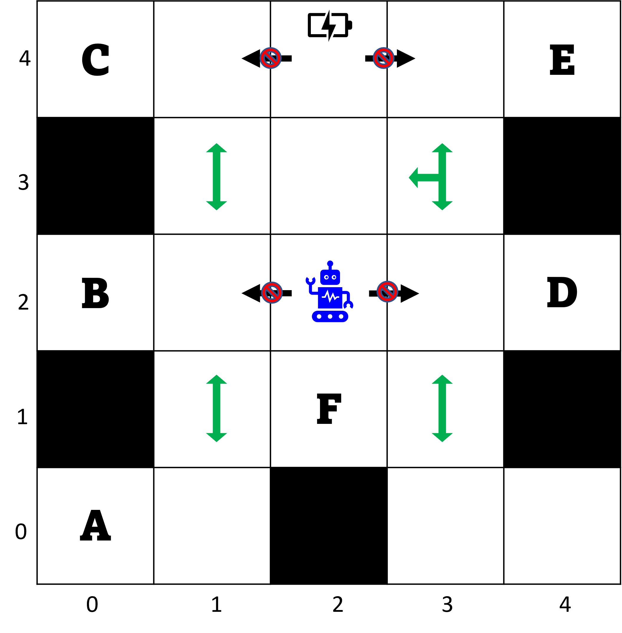
Figure 2: A gridworld example in which the black arrows with no-entry symbol denotes the disabled actions from that state and green arrows show the random outcomes on entering the cell.

Note that the preference model given to the robot is incomplete as well as combinative. It is incomplete because picking up items $A,B,C$ are mutually incomparable outcomes. Similarly, picking up items $D,E,F$ are mutually incomparable. It is combinative because, for instance, any play in which robot picks up an item from $D$ or $E$ is considered preferred to a play in which robot only picks an item from $A$ or $B$, even though to pick an item from $D$ or $E$ an item from $A$ or $B$ must be picked first.

We implemented the example in Python 3.9 on a Windows 10 machine with a core i$7$, 2.80GHz CPU and a 32GB memory. We discuss few noteworthy observations next. The MDP for this case has $3600$ states and $18496$ transitions, whereas the improvement MDP has $7200$ states and $35524$ transitions.

Consider the initial state $s_{0}=(2,2,8,(1,1,1,0,0,0,0))$ in which the robot is at cell $(2,2)$ with $8$ units of battery. The fourth component of the state denotes which items are available for pickup with the last element of the tuple reserved for availability of the charging station. In this state, the robot does not have an almost-sure winning strategy to visit any of $A,B$ or $C$. This is because to visit, say $A$, the robot must visit the slippery cell $(1,1)$. But whenever $(1,1)$ is visited, the robot may reach $(2,1)$ with a positive probability. Hence, $\mathsf{MP}(\mathsf{Outcomes}(s_{0}))=\emptyset$.

When under the SASI concept, the rank of the state $(s_{0},1)$ is $2$ indicating that two improvements are almost-surely guaranteed. This is understood by observing the SASI strategy which chooses action N at $(s_{0},0)$ to reach $s_{1}=(3,2,7,(1,1,1,0,0,0,0))$. At $(s_{1},0)$ the strategy selects W and visits either $B$ or $C$ with probability one. Since a pickup from $B$ and $C$ are incomparable, both actions N and S are deemed valid under SASI strategy at $(3,1,6,(1,1,1,0,0,0,0))$. On visiting either $B$ or $C$, the SASI strategy follows the almost-sure winning strategy to visit either $D$ or $E$ to make a second improvement. Since visiting the cell $(3,3)$ may result in returning back to the cell $(3,2)$ with a positive probability, the robot can recharge itself until a successful visit to $E$ or $D$ is made.

The SASI strategy at $(s_{0},0)$ does not select S because a second improvement cannot be guaranteed with probability one after visiting $A$ since the robot may remain at the cell $(0,1)$ until its battery runs out. However, we observe that the SPI strategy at $(s_{0},0)$ allows selection of both actions N, S at $(s_{0},0)$ since in both cases two improvements are possible with positive probability.

We conclude with Table I, which shows the number of states from which the robot has an SPI and SASI strategies to make at least $1$ or $2$ improvements, since the maximum number of improvements possible under given preference model is $2$. It is noted that the states from which a SASI strategy exists are a subset of states from which a SPI strategy exists.

	SASI	SPI
Rank-$1$	768	926
Rank-$2$	98	167

TABLE I: Number of states from which the robot has SPI and SASI strategies to make at least $1$ or at least $2$ improvements.

VII Conclusion

In this paper, we introduced two solution concepts, namely SPI and SASI to solve a preference-based planning problem given a combinative, incomplete preference model over infinite plays of a stochastic system. In the improvement MDP, we showed that the synthesis of SPI and SASI strategies reduces to that of computing positive and almost-sure winning strategies. Finally, we designed an algorithm using which we can synthesize a strategy that induces the maximum number of improvements under the SASI concept. Building on this work, there are a number of future directions: 1) it is possible to consider a preference over temporal objectives that encompass more general properties such as safety, recurrence, and liveness; 2) it remains open as how to connect qualitative reasoning with quantitative planning with such preference specifications.

References

- [1] R. Hastie and R. M. Dawes, Rational choice in an uncertain world: The psychology of judgment and decision making. Sage, 2010.
- [2] J. A. Baier and S. A. McIlraith, “Planning with Preferences,” AI Magazine, vol. 29, no. 4, p. 25, 2008.
- [3] T. C. Son and E. Pontelli, “Planning with preferences using logic programming,” Theory and Practice of Logic Programming, vol. 6, no. 5, pp. 559–607, 2006.
- [4] M. Bienvenu, C. Fritz, and S. A. McIlraith, “Specifying and computing preferred plans,” Artificial Intelligence, vol. 175, no. 7-8, pp. 1308–1345, 2011.
- [5] S. O. Hansson and T. Grüne-Yanoff, “Preferences”, the stanford encyclopedia of philosophy (spring 2022 edition).” [Online]. Available: https://plato.stanford.edu/archives/spr2022/entries/preferences/
- [6] H. Rahmani, A. N. Kulkarni, and J. Fu, “Probabilistic planning with partially ordered preferences over temporal goals,” arXiv preprint arXiv:2209.12267, 2022.
- [7] R. J. Aumann, “Utility theory without the completeness axiom,” Econometrica: Journal of the Econometric Society, pp. 445–462, 1962.
- [8] S. O. Hansson, The structure of values and norms. Cambridge University Press, 2001.
- [9] J. Tumova, G. C. Hall, S. Karaman, E. Frazzoli, and D. Rus, “Least-violating control strategy synthesis with safety rules,” in Proceedings of the 16th international conference on Hybrid systems: computation and control. ACM, 2013, pp. 1–10.
- [10] T. Wongpiromsarn, K. Slutsky, E. Frazzoli, and U. Topcu, “Minimum-violation planning for autonomous systems: Theoretical and practical considerations,” in 2021 American Control Conference, 2021, submitted.
- [11] H. Rahmani and J. M. O’Kane, “What to do when you can’t do it all: Temporal logic planning with soft temporal logic constraints,” in 2020 IEEE/RSJ International Conference on Intelligent Robots and Systems (IROS). IEEE, 2020, pp. 6619–6626.
- [12] N. Mehdipour, C.-I. Vasile, and C. Belta, “Specifying User Preferences Using Weighted Signal Temporal Logic,” IEEE Control Systems Letters, vol. 5, no. 6, pp. 2006–2011, Dec. 2021.
- [13] M. Lahijanian and M. Kwiatkowska, “Specification revision for Markov decision processes with optimal trade-off,” in Proc. 55th Conference on Decision and Control (CDC’16), 2016, pp. 7411–7418.
- [14] M. Li, A. Turrini, E. M. Hahn, Z. She, and L. Zhang, “Probabilistic preference planning problem for markov decision processes,” IEEE transactions on software engineering, 2020.
- [15] J. Fu, “Probabilistic planning with preferences over temporal goals,” in 2021 American Control Conference (ACC). IEEE, 2021, pp. 4854–4859.
- [16] G. R. Santhanam, S. Basu, and V. Honavar, “Representing and Reasoning with Qualitative Preferences: Tools and Applications,” Synthesis Lectures on Artificial Intelligence and Machine Learning, vol. 10, no. 1, pp. 1–154, Jan. 2016, zSCC: 0000006 Publisher: Morgan & Claypool Publishers. [Online]. Available: https://www.morganclaypool.com/doi/10.2200/S00689ED1V01Y201512AIM031
- [17] O. Kupferman and M. Y. Vardi, “Model checking of safety properties,” Formal methods in system design, vol. 19, no. 3, pp. 291–314, 2001.
- [18] C. Baier and J.-P. Katoen, Principles of model checking. MIT press, 2008.
- [19] D. Bouyssou, D. Dubois, and M. Pirlot, Concepts & Methods of Decision-Making. John Wiley & Sons Inc., 2009.
- [20] L. de Alfaro and R. Majumdar, “Quantitative solution of omega-regular games,” in Proceedings of the thirty-third annual ACM symposium on Theory of computing, 2001, pp. 675–683.
- [21] K. Chatterjee and T. A. Henzinger, “A survey of stochastic -regular games,” Journal of Computer and System Sciences, vol. 78, no. 2, pp. 394–413, 2012.