The Missing Link Between Black Holes in High-Mass X-ray Binaries and Gravitational-Wave Sources:
Observational Selection Effects

Abstract

There are few observed high-mass X-ray binaries (HMXBs) that harbor massive black holes, and none are likely to result in a binary black hole (BBH) that merges within a Hubble time; however, we know that massive merging BBHs exist from gravitational-wave observations. We investigate the role that X-ray and gravitational-wave observational selection effects play in determining the properties of their respective detected binary populations. We find that, as a result of selection effects, detectable HMXBs and detectable BBHs form at different redshifts and metallicities, with detectable HMXBs forming at much lower redshifts and higher metallicities than detectable BBHs. We also find disparities in the mass distributions of these populations, with detectable merging BBH progenitors pulling to higher component masses relative to the full detectable HMXB population. Fewer than $3\%$ of detectable HMXBs host black holes $>35M_{\odot}$ in our simulated populations. Furthermore, we find the probability that a detectable HMXB will merge as a BBH system within a Hubble time is $\simeq 0.6\%$. Thus, it is unsurprising that no currently observed HMXB is predicted to form a merging BBH with high probability.

1 Introduction

Current gravitational-wave (GW) sources consist of merging double compact objects with neutron star (NS) or black hole (BH) components (Abbott et al., 2019, 2021a, 2021b, 2022a). Their progenitors are important markers of binary evolution, as they provide information on the origin of DCOs and inform which evolutionary scenarios dominate their formation (Podsiadlowski et al., 2003; Tauris & Heuvel, 2003; Kratter, 2011; Miller & Miller, 2015; Heuvel, 2018; Abbott et al., 2016b). Such progenitors include high-mass X-ray binaries, which are binary systems that contain a massive OB-type donor star with an accreting compact object (CO) that can be either a NS or a BH (e.g., Verbunt, 1993; Remillard & McClintock, 2006). The donor star in HMXB systems is massive enough to itself form a CO, making HMXBs prime candidates for the progenitors of GW sources detectable by current ground-based detectors.

HMXBs are predominantly wind fed, meaning the accretion process is fueled by the stellar wind of the donor star (Blondin & Owen, 1997). At its simplest level, accretion can be modeled using the classical Bondi–Hoyle method (Bondi & Hoyle, 1944) and drives X-ray emission that can be observed with contemporary X-ray surveys (e.g., Oh et al., 2018; Krivonos et al., 2021; Pavlinsky et al., 2021; Predehl et al., 2021). When accretion is Eddington-limited, the X-ray accretion luminosity is also limited, e.g., emission is limited to $\sim 10^{39}~{}\mathrm{erg\,s}^{-1}$ for a $10~{}M_{\odot}$ BH accretor. All observed wind-fed HMXBs with confirmed BH accretors have high Roche lobe filling factors (Orosz et al., 2007, 2009; Miller-Jones et al., 2021), which means that these systems could soon begin Roche lobe overflow mass transfer. High Roche lobe filling factors may also be important in determining which HMXBs are detectable, as they are critical in forming focused accretion streams that drive BH disk formation (Hirai & Mandel, 2021).

Approximately $80$ Galactic HMXBs have been observed, but not all systems have well-constrained binary properties (Krivonos et al., 2012; Clavel et al., 2019; Kretschmar et al., 2019). Most of these HMXBs are thought to have BH accretors, but the majority have yet to be dynamically confirmed with spectroscopic observations (Motta et al., 2021). Cyg X-1, a Galactic HMXB containing the first-ever dynamically confirmed stellar-mass BH (Bolton, 1972; Webster & Murdin, 1972), is estimated to contain a $21.2^{+2.2}_{-2.2}~{}M_{\odot}$ BH accretor and a ${40.6^{+7.7}_{-7.1}~{}M_{\odot}}$ main-sequence donor (Miller-Jones et al., 2021). Another well-studied Galactic HMXB is Cyg X-3, which is estimated to contain a CO accretor of $2.4^{+2.1}_{-1.1}~{}M_{\odot}$ and a Wolf–Rayet donor of $10.3^{+3.9}_{-2.8}~{}M_{\odot}$ (Zdziarski et al., 2013). While the mass of the accretor falls near the maximum mass allowed by the uncertain NS equation of state (Lattimer, 2021), radio, infrared and X-ray properties of the system suggest that it is a low-mass BH (Zdziarski et al., 2013). Thus, of the few Galactic HMXBs that have well-constrained binary properties, only Cyg X-1 is thought to contain a BH $\gtrsim 20M_{\odot}$.

Observational campaigns throughout the past two decades have uncovered a large number of extragalactic HMXB candidates (e.g., Fabbiano, 2006; Haberl & Sturm, 2016; Lazzarini et al., 2018; Rice et al., 2021). Of these sources, one of the few that has well-resolved binary properties is LMC X-1, the brightest X-ray source in the Large Magellanic Cloud (Mark et al., 1969). Orosz et al. (2009) estimate it to have a donor mass of $(31.8\pm 3.5)~{}M_{\odot}$ and a BH accretor mass of $(10.9\pm 1.4)~{}M_{\odot}$. Another resolved extragalactic HMXB is M33 X-7, an HMXB in the spiral galaxy M33 estimated to have a $38^{+22}_{-10}M_{\odot}$ donor star and a $11.4^{+3.3}_{-1.7}~{}M_{\odot}$ BH (Ramachandran et al., 2022). Similar to Galactic HMXBs, the population of well-constrained extragalactic sources is small, and in this case none are found to harbor BH accretors $>20~{}M_{\odot}$.

In addition to dynamically-observed BHs in HMXBs, many stellar-mass BHs have been discovered with the Laser Interferometer Gravitational-Wave Observatory (LIGO; Aasi et al., 2015) and Virgo (Acernese et al., 2015) GW detectors as DCO mergers (Abbott et al., 2016a, 2021b). The global GW detector network made the first observation of GWs from a merging binary black hole (BBH) with component masses of $34.6^{+4.4}_{-2.6}~{}M_{\odot}$ and $30.0^{+2.9}_{-4.6}~{}M_{\odot}$ in 2015 (Abbott et al., 2016a, 2022a). The Laser Interferometer Gravitational-Wave Observatory (LIGO) Scientific, Virgo and KAGRA Collaboration has identified $90$ probable DCO merger candidates during their first three observing runs (Abbott et al., 2019, 2021a, 2022a, 2021b), including two sources that have component masses consistent with a NS–NS merger (Abbott et al., 2017, 2020a) and a few sources with component masses consistent with a NS–BH merger (Abbott et al., 2020c, 2021b, 2021c, 2022a).

Using GW observations, population analyses are able to constrain aspects of the underlying BBH mass distribution, with the most recent analyses identifying substructure in the mass distribution beyond the simplest phenomenological models (Tiwari & Fairhurst, 2021; Abbott et al., 2022b; Edelman et al., 2022). The global peak of the mass distribution is at $\simeq 10M_{\odot}$, and there is strong evidence of a secondary peak at $\simeq 35M_{\odot}$. Though there is clear support for masses above what would be allowed for a simple power law with a cutoff, the $99$th percentile of the underlying mass distribution is $44^{+9.2}_{-5.1}M_{\odot}$ (Abbott et al., 2022b). Distributions of BH source properties, such as their mass, can be used to probe the astrophysics of BBH formation and evolution (Belczynski et al., 2016; Barrett et al., 2018; Fishbach et al., 2020; Zevin et al., 2021; Mandel & Farmer, 2018).

Since HMXBs will potentially form DCOs, they are prime candidates for the progenitors of compact binary mergers detected via GWs. However, there is uncertainty as to whether HMXB progenitors significantly contribute to the merging compact binary population. For example, the HMXB donor star and CO may merge later in their evolution before becoming a compact binary, get disrupted during the supernova that forms the second CO, or have too wide of an orbital separation at DCO formation to merge within a Hubble time.

Several studies have been conducted to predict the fate of observed HMXBs. Neijssel et al. (2021) predict the fate of Cyg X-1 with its updated BH and donor star mass estimates from Miller-Jones et al. (2021) by evolving it forward with the COMPAS population synthesis code (Riley et al., 2022). They find that the system will most likely form a BH–NS binary that has a $\simeq 7\%$ chance of remaining bound after the NS natal kick. With revised models of mass transfer and natal kicks that produce heavier donor remnant masses, Neijssel et al. (2021) predict that Cyg X-1 could potentially form a BBH albeit at a low probability; in these scenarios, they find the probability Cyg X-1 will merge as a BBH within a Hubble time is $\simeq$ 4–5%. Similar studies have been done for LMC X-1 (Belczynski et al., 2012) and Cyg X-3 (Belczynski et al., 2013). Of these two binaries, only Cyg X-3 is predicted to potentially merge as a BBH within a Hubble time, although this outcome heavily relies on where the component masses fall within the measured observational uncertainties as well as the assumed models of binary evolution. Thus, it is unlikely that any currently observed HMXBs will form merging BBHs within a Hubble time.

In addition to the lack of currently observed HMXBs that are thought to be merging BBH progenitors, there are differences in the BH masses of the observed HMXB and merging BBH populations. While the primary BH mass distribution predicted from GW observations extends to masses higher than the peak near $35M_{\odot}$ (Abbott et al., 2022b), there are no observed HMXBs with BH accretor masses that fall near or beyond this limit. Rather than arising from fundamental astrophysical differences, the disparities in the observed HMXB and GW BH population masses may actually be a product of detector selection effects alone. Fishbach & Kalogera (2022) compare the observed mass distributions of BHs in HMXBs and BHs observed with GWs, and find that when GW detector selection effects are accounted for, there are currently no statistically significant mass differences between the HMXB and GW BH populations. However, it is critical that X-ray and GW observational selection effects are jointly examined, as they may produce differing outcomes in the observed populations.

The spin distributions of X-ray and GW BH populations can also provide insight on their evolutionary history and the role of selection effects in determining their properties. Fishbach & Kalogera (2022) examine the BH spin distributions of BH–HMXBs and GW–BBHs and find them to be inconsistent with one another. It is possible, however, that differing binary evolutionary channels between the two populations may contribute to this discrepancy. For example, Gallegos-Garcia et al. (2022) find that high-spin HMXBs formed through Case-A mass transfer can only form merging BBHs within a small parameter space, and thus it is not surprising that the observed spin distributions are observed to be different.

In this paper, we show that observational selection effects play an important role in determining the observed BH population masses and the evolutionary predictions of detected HMXBs. We compare detectable HMXB populations with detectable GW populations using simulated astrophysical samples of binaries, and we quantify the probability that detectable HMXBs will form BH–BH binaries that will merge in a Hubble time, accounting for X-ray selection effects. We do not attempt to reproduce HMXB or GW observations in detail; rather, we seek to understand how observational selection effects may produce the aforementioned differences in mass ranges and evolutionary predictions of HMXBs.

In Section 2, we discuss our methods for sampling populations of binaries distributed throughout the universe, as well as how we model their X-ray and GW emission properties. We develop a formalism for quantifying the probability of obtaining a given source in our sampled population, taking into account observational selection effects. In Section 3, we discuss parameter distribution properties for detectable HMXBs and detectable merging BBHs in our sample, as well as evolutionary probabilities for these sources. Finally, in Section 4, we discuss our main results, caveats in our analysis, and the implications of our findings in the context of X-ray and GW observations. Throughout this work, we assume Planck 2018 cosmological parameters (Aghanim et al., 2020), including values for the Hubble constant ($H_{0}=67.7\,\mathrm{km}\,\mathrm{s}^{-1}\mathrm{Mpc}^{-1}$) and the mass and dark energy density parameters ($\Omega_{\mathrm{m}}=0.31$ and $\Omega_{\Lambda}=0.69$, respectively). All data and code files supporting the findings reported in this paper are provided as supplementary information on Zenodo and Github, respectively.

2 Methods

We examine populations of HMXBs with the rapid binary population synthesis code COSMIC (version 3.4; Breivik et al., 2020). COSMIC is based on the single-stellar evolution formulae from Hurley et al. (2000) and the binary evolution prescriptions from Hurley et al. (2002). COSMIC includes many updates to these prescriptions, such as those for OB stellar winds (Vink et al., 2001), Wolf–Rayet star winds (Vink & de Koter, 2005), the initiation of unstable mass transfer (Belczynski et al., 2008; Claeys et al., 2014; Neijssel et al., 2019), remnant formation (Fryer et al., 2012), and pair instability supernovae (Woosley, 2017; Marchant et al., 2019; Spera et al., 2019). We generate binary populations with COSMIC across a grid of metallicities, and then sample systems from these populations and distribute them across redshifts.

2.1 Binary Population Models

We use COSMIC to generate populations of HMXBs. To do this, we allow the formation of DCOs where the first-born object is a BH or NS and the second-born object is a white dwarf (WD), NS, or BH. We only keep binaries that remain bound after the first supernova (SN) event and have stellar companion masses $>5M_{\odot}$ at the formation time of the first-born CO. We make these cuts because we define HMXBs to be systems that are concurrently bound and contain one accreting CO and one stellar object $\geq$ 5 $M_{\odot}$ at some point in their evolution. These cuts ensure that our initial sample space allows for HMXB formation but is not restricted to only merging BBH progenitors.

We simulate 16 DCO populations across a discrete log-spaced metallicity grid that spans $(1/200)Z_{\odot}$ to $(7/4)Z_{\odot}$, as this metallicity range is approximately that of the grids used for stellar evolution within COSMIC (Hurley et al., 2000). Our population models include a set of key assumptions. We draw primary masses using the initial mass function from Kroupa (2001), and initial orbital periods and eccentricities following the prescriptions from Sana et al. (2012). We fix the binary fraction to be 0.7. We limit the minimum mass ratio to be set such that the pre-main sequence lifetime of the secondary is not longer than the full lifetime of the primary if it were to evolve as a single star. We assume a solar metallicity of $Z_{\odot}=0.017$ (Grevesse & Sauval, 1998) for all calculations. To calculate CO remnant properties from the pre-supernova properties of a star, we employ the Delayed remnant mass prescription from Fryer et al. (2012) that allows for CO formation in the lower mass gap (e.g., Zevin et al., 2020). We assume a conservative upper-limit for the maximum NS mass of $3~{}M_{\odot}$ (Rhoades & Ruffini, 1974; Kalogera & Baym, 1996). To determine respective remnant masses for pulsational pair-instability supernovae and pair-instability supernovae, we use fits to Table 1 of Marchant et al. (2019). For common-envelope evolution, we use the prescription from Belczynski et al. (2008) to determine the critical mass ratio for the onset of unstable mass transfer. We set $\alpha=1$ for the common-envelope efficiency parameter (Livio & Soker, 1988; Ivanova et al., 2013), and use a variable prescription for the envelope binding energy factor $\lambda$ (Claeys et al., 2014). Last, we set the wind-accretion efficiency factor to $0.5$, and enforce Eddington-limited accretion in all binaries.

These assumptions represent a single fiducial point in a high-dimensional parameter space of binary evolution uncertainties that can have a significant impact on the population properties of compact binaries and their progenitors (e.g., Barrett et al., 2018; Belczynski et al., 2022; Broekgaarden et al., 2022). Because we do not attempt to reproduce observations in detail and rather seek to understand how selection effects impact HMXB and merging BBH populations, a fiducial model is satisfactory for our purposes. We reserve a more systematic exploration of this parameter space for future work, and we comment on possible impacts to our results in Section 4.

2.2 Population Sampling

From our set of COSMIC models run at discrete metallicities, we sample two populations of binaries: the first is a local population sampled out to redshift 0.05 (denoted $z_{<0.05}$), and the second is a population sampled out to redshift 20 (denoted $z_{<20}$). Because our COSMIC populations assume a single burst of star formation and evolve all systems for a Hubble time, we must assign binary redshifts and metallicities in postprocessing. We sample a $z_{<0.05}$ population to acquire robust detectable HMXB population statistics that cannot be acquired in a $z_{<20}$ sample, as the effective sample size of detectable HMXBs in the $z_{<20}$ population is small (there are $\simeq 100$ detectable HMXBs in the $z_{<20}$ sample compared to $\simeq 7\times 10^{3}$ in the $z_{<0.05}$ sample). Our choice to use a locally-sampled population of HMXBs in our analysis is discussed in more detail in Section 3.1.

We draw redshifts and metallicites jointly from a two-dimensional redshift–metallicity grid using the weights

$$\mathcal{W}(z,Z)=\zeta(Z)P(Z|z)\psi[z(t)]\ \frac{\mathrm{d}t}{\mathrm{d}z}.$$ (1)

Here, $\zeta(Z)$ is the number of HMXBs formed per unit stellar mass formed at metallicity $Z$; $P(Z|z)$ is the probability of drawing metallicity $Z$ at redshift $z$; $\psi[z(t)]$ is the star formation rate at redshift $z$ attained by marginalizing over metallicity in a grid of stellar mass formed per unit lookback time and metallicity, and the term $\mathrm{d}t/\mathrm{d}z$ is to change of variables from time to redshift space for $\psi[z(t)]$,

$$\frac{\mathrm{d}t}{\mathrm{d}z}=\frac{1}{(1+z)E(z)},$$ (2)

where $E(z)$ is the cosmological factor for a flat universe (Ryden, 2002),

$$E(z)=\sqrt{\Omega_{\mathrm{m}}(1+z)^{3}+\Omega_{\nu}(1+z)^{4}+\Omega_{\Lambda}}.$$ (3)

We determine $P(Z|z)$ using publicly-available data from the Illustris-TNG simulation (Nelson et al., 2019). This simulation provides stellar mass formed per unit lookback time and metallicity in a $100~{}\mathrm{Mpc}^{3}$ comoving box (Zevin & Bavera, 2022, Section 2.3). The bounds of the distribution for $P(Z|z)$ are $Z/Z_{\odot}=5\times 10^{-5}$ and $Z/Z_{\odot}=0.04$, which approximately correspond to the lower and upper bounds of our COSMIC population metallicity grid. Though the redshift–metallicity evolution $P(Z|z)$ is highly uncertain, especially at high redshifts, the star formation rate density evolution predicted from Illustris-TNG falls within the range of uncertainty (e.g., Chruślińska, 2022), and the evolution of the metallicity distribution is more astrophysically motivated than analytic approaches, such as truncated log-normal distributions.

We jointly draw $N_{\mathrm{total}}=10^{6}$ redshifts and metallicities using the relative weights from Eq. (1), and randomly sample binaries from the discrete COSMIC metallicity models based on which discrete metallicity model is closest to a drawn metallicity in log-space. This provides a DCO population distributed across metallicity and redshift that is representative of a population of binaries in the universe.

2.3 X-Ray Binary Detection Flux

As we are interested in binaries that can potentially lead to BBH mergers, we consider BH–HMXBs in our sample to be systems that are concurrently bound and contain one BH object and one stellar object $\geq$ 5 $M_{\odot}$ at some point in their evolution. The X-ray binary (XRB) phase begins at first BH formation and ends at second CO formation or when the donor mass falls below 5 $M_{\odot}$.

Since the time series resolution needed to calculate the X-ray emission of HMXBs is much finer than what COSMIC can handle for large populations, we re-evolve HMXBs in our sample with a small timestep resolution of $10^{3}$ years. We only apply this fine resolution during the HMXB phase to ensure computational efficiency. This is possible due to the ability of COSMIC to restart binaries in the middle of their evolution and evolve them forward (Breivik et al., 2020).

We adopt the method from Podsiadlowski et al. (2003) to calculate the HMXB accretion luminosity,

$$L_{\mathrm{acc}}=\eta\dot{M}_{\mathrm{acc}}c^{2},$$ (4)

where $\dot{M}_{\mathrm{acc}}$ is the Eddington-limited accretion rate of matter onto the BH and $\eta$ is an efficiency factor for the BH conversion of rest mass into radiative energy. For simplicity, we calculate $\eta$ assuming zero initial BH spin and that it is determined entirely by the last stable particle orbit. For $M_{\mathrm{BH}}<\sqrt{6}M_{\mathrm{BH},0}$, the efficiency $\eta$ is

$$\eta=1-\sqrt{1-\bigg{(}\frac{M_{\mathrm{BH}}}{3M_{\mathrm{BH},0}}\bigg{)}^{2}},$$ (5)

where $M_{\mathrm{BH}}$ is the BH mass at a given time and $M_{\mathrm{BH},0}$ is the initial BH gravitating mass–energy at formation according to Bardeen (1970). If $M_{\mathrm{BH}}$ exceeds $\sqrt{6}M_{\mathrm{BH},0}$, then $\eta$ is taken to be 0.42. The accretion rate is related to the change in BH mass by

$$\dot{M}_{\mathrm{BH}}=(1-\eta)\dot{M}_{\mathrm{acc}},$$ (6)

as energy released as radiation will not contribute to the BH mass. COSMIC includes wind prescriptions for mass loss in its evolution, so we do not need to explicitly calculate wind accretion. All changes in BH mass from both Roche lobe overflow and wind mass transfer are included in $\dot{M}_{\mathrm{BH}}$.

To determine if a given HMXB is detectable, we impose a flux limit for observations. The X-ray flux is

$$F=\frac{L_{\mathrm{acc}}}{4\pi D_{\mathrm{L}}(z)^{2}},$$ (7)

where $D_{\mathrm{L}}(z)$ is the luminosity distance of the binary at the start of the HMXB phase. An HMXB is considered detectable when its flux exceeds $5\times 10^{-15}$ erg s^-1 cm^-2, which is an observational threshold commonly used in X-ray surveys (e.g., Chandra X-ray Center et al., 2021).

2.4 Gravitational-Wave Detection Probability

We calculate the GW detection probabilities $p_{\mathrm{det}}$ of DCO binaries in our sample that have merged by today ($z=0$). We evaluate the source signal-to-noise ratio (S/N) $\rho$ as

$$\rho=\rho_{0}\omega,$$ (8)

where $\rho_{0}$ is the maximal S/N of a face-on, overhead source with component masses $m_{1}$ and $m_{2}$ at redshift $z$, and $\omega$ is a projection factor that depends on the relative angular orientation of the source and the detector (Dominik et al., 2015).

We approximate $\rho_{0}$ following Fishbach et al. (2018) as

$$\rho_{0}=8\left[\frac{\mathcal{M}(1+z_{\mathrm{m}})}{\mathcal{M}_{8}}\right]^{5/6}\frac{D_{\mathrm{L},8}}{D_{\mathrm{L}}},$$ (9)

where $\mathcal{M}=(m_{1}m_{2})^{3/5}/(m_{1}+m_{2})^{1/5}$ is the source chirp mass, $D_{\mathrm{L}}$ is the luminosity distance of the source, $z_{\mathrm{m}}$ is the merger redshift, and the constants $\mathcal{M}_{8}$ and $D_{\mathrm{L},8}$ are set to $10\;M_{\odot}$ and $1~{}\mathrm{Gpc}$, respectively, such that they represent the typical distances (Chen et al., 2021) at which sources are detectable by Advanced LIGO at design sensitivity (Aasi et al., 2015). This scaling approximates the amplitude of a GW coalescence signal to first order. For the projection factor $\omega$, we use the analytical expression for a single-detector network from Dominik et al. (2015), which is equivalent to $\Theta/4$ in Finn & Chernoff (1993). We calculate the detection probability $p_{\mathrm{det}}$ by Monte Carlo sampling $\omega$ and taking the fraction of the resulting source S/N that exceed a detection threshold of $\rho=8$ (Thorne, 1997; Chen et al., 2021).

2.5 Population Probabilities

We are interested in calculating the probability of obtaining sources in our sampled populations. In the most general form, we define the probability of finding a given source in state $X$ in our sample as

$$P({X})=\frac{N_{X}}{N_{\mathrm{total}}},$$ (10)

where $N_{X}$ is the number of sources in state $X$ and $N_{\mathrm{total}}$ is the number of sources in the full sample of interest. Because we need to count sources with different lifetimes distributed across space and time relative to an observer, a more involved framework is necessary to obtain values for $N_{X}$ and $N_{\mathrm{total}}$.

We first need to count the number of binaries of interest $N_{X}$ in a given spatial comoving volume $V_{\mathrm{c}}$ with spatial points $\vec{x}$ surveyed from comoving times $t_{1}=t_{1}(\vec{x})$ to $t_{2}=t_{2}(\vec{x})$ in the source frame. Each source in a small spatial density of sources $n(\vec{x},t)$ has its own worldline along which it may be in some state $X$ for some time, which we track with an indicator function $I(\vec{x},t)$ that is nonzero when in state $X$ and zero otherwise, and normalized such that for a single source $\int\int I(\vec{x},t)\,\mathrm{d}t\mathrm{d}\vec{x}=1$. Thus, we count the number of systems in state $X$ as

$$N_{X}=\int_{V_{\mathrm{c}}}\int_{t_{1}(\vec{x})}^{t_{2}(\vec{x})}{n(\vec{x},t)I(\vec{x},t)}\,\mathrm{d}t\mathrm{d}\vec{x}.$$ (11)

2.5.1 Long-lived Sources

For any type of source whose lifetime is significantly longer than the length of the observing window ${T=(t_{2}-t_{1})}$, the number of counted sources $N_{\mathrm{long}}$ does not change during the observing period. This implies that the spatial density is only a function of position $n(\vec{x})$. The indicator function takes on a form $I(x)/T$, and all observing-time dependence disappears after integrating over time. One instance where this is the case is with detectable HMXBs. As detailed in Section 3.1, even HMXBs that emit above the X-ray detection threshold for a comparatively short amount of time emit on the order of thousands of years, making it valid to count them as long-lived sources compared to the timescale of astronomical surveys. This long-lived limit also holds for binaries that exist in some evolutionary state for a significant length of time, e.g., bound BBHs that have not merged.

With this simplification considered, we now count the number of long-lived sources as

$$N_{\mathrm{long}}=\int_{V_{\mathrm{c}}}n(\vec{x})\,\mathrm{d}\vec{x}.$$ (12)

This equation can be rewritten in terms of redshift,

$$N_{\mathrm{long}}=\int_{z_{1}}^{z_{2}}n(z)\frac{\mathrm{d}V_{\mathrm{c}}}{\mathrm{d}z}\mathrm{d}z,$$ (13)

where the redshifts $z_{1},z_{2}$ are the bounds of the volume $V_{\mathrm{c}}$, $n(z)$ is the number density of sources in terms of redshift, and the factor $\mathrm{d}V_{\mathrm{c}}/\mathrm{d}z$ is the comoving volume element corresponding to redshift $z$, which is given by (Ryden, 2002),

$$\frac{\mathrm{d}V_{\mathrm{c}}}{\mathrm{d}z}=\frac{4\pi c}{H_{0}}\frac{D_{\mathrm{c}}(z)^{2}}{E(z)},$$ (14)

where $D_{\mathrm{c}}(z)$ is the comoving distance at redshift $z$ and $E(z)$ is defined in Eq. (3). Changing variables from spatial coordinates to redshift significantly simplifies the evaluation of the integral for $N_{\mathrm{long}}$.

Since we use a discrete simulation for our calculations, Eq. (13) must be approximated as a discrete sum over individual sources in our COSMIC populations and a Riemann sum over redshift,

$$N_{\mathrm{long}}=\sum_{i}\sum_{j}\frac{I_{i}^{X}(z_{j})}{V_{\mathrm{box}}}\frac{\mathrm{d}V_{\mathrm{c}}}{\mathrm{d}z_{j}}\Delta z_{j},$$ (15)

where we have re-written the spatial density of sources as $n(z_{j})=\sum_{i}I_{i}^{X}(z_{j})/V_{\mathrm{box}}$. Here, $I_{i}^{X}(z_{j})$ indicates if the $i$-th system in the sample is in state $X$ at redshift $z_{j}$, and $V_{\mathrm{box}}$ is the volume of the comoving box that we consider for our resampled population. Eq. (15) allows for a quick, simplified computation of $N_{\mathrm{long}}$.

2.5.2 Short-lived Sources

We can also apply Eq. (11) to calculate the number of sources $N_{\mathrm{short}}$ in the case that their lifetimes are significantly shorter than the length of the observing window. This includes BBH mergers in the frequency band of ground-based GW detectors which only exist as detectable sources for at most a few seconds before coalescence. In this case, the length of the source lifetime approaches zero, which causes the indicator function to act as a delta function,

$$N_{\mathrm{short}}=\int_{V_{\mathrm{c}}}\int_{t_{1}(\vec{x})}^{t_{2}(\vec{x})}n(\vec{x},t)\delta(t-t^{\prime}(\vec{x}))\,\mathrm{d}t\mathrm{d}\vec{x},$$ (16)

where $t^{\prime}(\vec{x})$ marks the time at which state $X$ occurs at spatial position $\vec{x}$. In the continuum limit, this expression is an integral over the rate density of sources $r(\vec{x},t)$,

$$N_{\mathrm{short}}=\int_{V_{\mathrm{c}}}\int_{t_{1}(\vec{x})}^{t_{2}(\vec{x})}r(\vec{x},t)\,\mathrm{d}t\mathrm{d}\vec{x}.$$ (17)

When we observe for some time window $T$, the time dependence of the rate density in Eq. (17) integrates to $T$ with a factor of $1/(1+z)$ to account for transitioning between the source frame and observer frame time. As with Eq. (13), we use a change of variables to write the volume integral as an integral over redshift,

$$N_{\mathrm{short}}=T\int_{z_{1}}^{z_{2}}r(z)\frac{\mathrm{d}V_{\mathrm{c}}}{\mathrm{d}z}\frac{1}{1+z}\mathrm{d}z.$$ (18)

where $r(z)$ is the rate density of sources as a function of redshift. Rewriting this equation as a sum over individual sources, we obtain

$$N_{\mathrm{short}}=T\sum_{i}\sum_{j}\frac{I_{i}^{X}(t_{j},t_{j}+\tau)}{\tau V_{\mathrm{box}}}\frac{\mathrm{d}V_{\mathrm{c}}}{\mathrm{d}z_{j}}\frac{1}{1+z_{j}}\Delta z_{j},$$ (19)

where we have re-written the rate density of sources as $r(t_{j})=\sum_{i}I_{i}^{X}(t_{j},t_{j}+\tau)/[\tau V_{\mathrm{box}}]$, with $t_{j}=t(z_{j})$. $I_{i}^{X}(t_{j},t_{j}+\tau)$ indicates if the $i$-th system in the sample undergoes an event $X$ at redshift $z_{j}$ between times $t_{j}$ and $t_{j}+\tau$, where $\tau$ is a chosen time interval significantly shorter than the timescale on which the rate density evolves. For practical purposes, $\tau$ can be thought of as a chosen bin width in time. Eq. (19) allows for an efficient computation of $N_{\mathrm{short}}$.

2.5.3 Detection Weights

We apply the formalism developed in the previous subsections to assign relative detection weights to all binaries in our sample. Specifically, the sums over redshift in Eq. (15) and Eq. (19) are the expressions we use to define the weight of source $i$ in state $X$. As we consider relative weights, we can ignore the constant volume factor $V_{\mathrm{box}}$ and the time factors $T$ and $\tau$. We use the formalism for long-lived sources to calculate detectable HMXB weights, and that for short-lived sources to calculate detectable GW weights.

For HMXB sources that emit for long times, this weighting is the sum over redshift in Eq. (15), which becomes

$$\mathcal{W}_{\mathrm{xrb},i}\propto\sum_{j}I_{i}^{\mathrm{HMXB}_{\mathrm{obs}}}(z_{j})\frac{\mathrm{d}V_{\mathrm{c}}}{\mathrm{d}z_{j}}\Delta z_{j},$$ (20)

where the indicator $I^{\mathrm{HMXB}_{\mathrm{obs}}}(z_{j})$ has value equal to unity if the HMXB exceeds a given X-ray detection threshold at redshift $z_{j}$, and has value zero otherwise. Thus, sources that emit above the detection threshold for longer periods of time will contribute more in the summation and be given a higher relative detection weighting.

The weights for merging BBH sources are similar, but now the GW detection probability is included with the indicator function to account for selection effects,

$$\mathcal{W}_{\mathrm{gw},i}\propto\sum_{j}I_{i}^{\mathrm{BBH}_{\mathrm{m}}}(z_{j})p_{\mathrm{det},i}\frac{\mathrm{d}V_{\mathrm{c}}}{\mathrm{d}z_{j}}\frac{1}{1+z_{j}}\Delta z_{j},$$ (21)

where the indicator $I_{i}^{\mathrm{BBH}_{\mathrm{m}}}(z_{j})$ has value unity if the BBH coalesces at redshift $z_{j}$ and zero otherwise. Thus, for BBHs merging at redshift $z_{m}$, each system has a relative weight of

$$\mathcal{W}_{\mathrm{gw},i}\propto p_{\mathrm{det},i}\frac{\mathrm{d}V_{\mathrm{c}}}{\mathrm{d}z_{m}}\frac{1}{1+z_{m}}\Delta z_{m}.$$ (22)

Building this formalism for relative detection weights allows us to easily compare detectable systems and their progenitors in Section 3.

2.5.4 Probability Expressions

We use the counting expressions in Section 2.5.1 and Section 2.5.2 to calculate probabilities in the form of Eq. (10). For detectable HMXBs, this equation becomes

$$P(\mathrm{HMXB}_{\mathrm{obs}})=\frac{N_{\mathrm{HMXB}_{\mathrm{obs}}}}{N_{\mathrm{total}}},$$ (23)

which, written in summation form, is

$$P(\mathrm{HMXB}_{\mathrm{obs}})=\frac{\sum_{i}\sum_{j}I_{i}^{\mathrm{HMXB}_{\mathrm{obs}}}(z_{j})[\mathrm{d}V_{\mathrm{c}}/\mathrm{d}z_{j}]\Delta z_{j}}{\sum_{i^{\prime}}\sum_{j^{\prime}}I_{i^{\prime}}^{\mathrm{ZAMS}}(z_{j^{\prime}})[\mathrm{d}V_{\mathrm{c}}/\mathrm{d}z_{j^{\prime}}]\Delta z_{j^{\prime}}},$$ (24)

where $I_{i^{\prime}}^{\mathrm{ZAMS}}(z_{j^{\prime}})$ indicates if the $i$-th system in the sample has been initialized at zero-age main-sequence (ZAMS) and exists as any form of bound binary at redshift $z_{j^{\prime}}$. These are the systems we count as members of the $N_{\mathrm{total}}$ sample of binaries.

For merging BBHs, the probability of detecting a source is

$$P(\mathrm{BBHm}_{\mathrm{obs}})=\\ \frac{T}{\tau}\frac{\sum_{i}\sum_{j}I_{i}^{\mathrm{BBHm}}(t_{j},t_{j}+\tau)p_{\mathrm{det},i}[{\mathrm{d}V_{\mathrm{c}}}/{\mathrm{d}z_{j}}][{1+z_{j}}]^{-1}\Delta z_{j}}{\sum_{i^{\prime}}\sum_{j^{\prime}}I_{i^{\prime}}^{\mathrm{ZAMS}}(z_{j^{\prime}})[{\mathrm{d}V_{\mathrm{c}}}/{\mathrm{d}z_{j^{\prime}}}]\Delta z_{j^{\prime}}}.$$ (25)

This probability heavily depends on choices for the observing window $T$ and the detector sensitivity described by $p_{\mathrm{det}}$, so it is primarily determined by survey details. The time $\tau$ is a choice of bin width in time for approximating time integrals. The probability $P(\mathrm{BBHm}_{\mathrm{obs}})$ is only loosely dependent on $\tau$, because $I_{i}^{\mathrm{BBHm}}(t_{j},t_{j}+\tau)$ scales approximately linearly with $\tau$, which counters the $\tau$ in the denominator.

We also consider conditional probabilities for sources in our sample. For example, the probability a detectable HMXB will become a BBH that merges within a Hubble time can be written as

$$P(\mathrm{BBHm}_{\mathrm{H}}|\mathrm{HMXB}_{\mathrm{obs}})=\frac{P(\mathrm{BBHm}_{\mathrm{H}}\cap\mathrm{HMXB}_{\mathrm{obs}})}{P(\mathrm{HMXB}_{\mathrm{obs}})},$$ (26)

which, in summation form, is

$$P(\mathrm{BBHm}_{\mathrm{H}}|\mathrm{HMXB}_{\mathrm{obs}})=\\ \frac{\sum_{i}\sum_{j}I_{i}^{\mathrm{HMXB}_{\mathrm{obs}}\cap\mathrm{BBHm}_{\mathrm{H}}}(z_{j})[{\mathrm{d}V_{\mathrm{c}}}/{\mathrm{d}z_{j}}]\Delta z_{j}}{\sum_{i^{\prime}}\sum_{j^{\prime}}I_{i^{\prime}}^{\mathrm{HMXB}_{\mathrm{obs}}}(z_{j^{\prime}})[{\mathrm{d}V_{\mathrm{c}}}/{\mathrm{d}z_{j^{\prime}}}]\Delta z_{j^{\prime}}},$$ (27)

where $I_{i}^{\mathrm{HMXB}_{\mathrm{obs}}\cap\mathrm{BBHm}_{\mathrm{H}}}(z_{j})$ indicates if the $i$-th system in the sample is an HMXB emitting above a given detection flux threshold at redshift $z_{j}$ that will also become a merging BBH within a Hubble time.

These probability expressions, along with those for the relative detection weights in Eq. (20) and Eq. (22), provide all the mathematical tools necessary to quantify the relationships between detectable sources and their progenitors.

3 Results

To determine the impact of X-ray and GW selection effects on their observed populations, we apply detection weights as calculated in Section 2.5.3 to our sampled binaries from COSMIC. To fully understand these results, we must also understand the emission behavior of our X-ray and GW populations. This provides context for their evolutionary behavior and how it relates to their detectability, especially in the HMXB case where emission behavior has not been well-characterized for large theoretical populations. We also examine the mass distributions of detected HMXB and BBH populations and calculate probabilities describing the relationships of sources to one another. Through this analysis, we illuminate possible causes of the observational discrepancies in BH masses and evolutionary predictions between X-ray and GW sources.

3.1 HMXB Emission Properties

The emission properties of our HMXB populations, as calculated in Section 2.3, provide insight into the nature of their detectability. Figure 1 shows the maximum X-ray luminosity $L_{\mathrm{max}}$ reached by all HMXBs in our $z_{<0.05}$ and $z_{<20}$ samples, as well as the time-averaged X-ray luminosity $L_{\mathrm{avg}}$ of HMXBs during the XRB phase for the $z_{<0.05}$ sample. We mark the Eddington luminosities for $10~{}M_{\odot}$ and $30~{}M_{\odot}$ BH accretors with vertical dotted lines. Almost $70\%$ of the $z_{<0.05}$ HMXBs achieve peak luminosities between $10^{38}$ and $10^{39}~{}\mathrm{erg\,s^{-1}}$ during their XRB phase, which is roughly within one order of magnitude of their Eddington luminosity. The overall maximum emission behavior of the $z_{<0.05}$ and $z_{<20}$ HMXBs is similar across all luminosities. Both exhibit a steep drop in the distribution close to the Eddington limit along with a tail to lower X-ray luminosities.

The time-averaged luminosity during the XRB phase follows approximately the same distribution as the maximum luminosity for values $<10^{33}~{}\mathrm{erg\,s^{-1}}$. At higher luminosities, however, these distributions diverge, with a larger discrepancy between the average and maximum luminosities reached during the XRB phase. This is because in our models, most systems emitting at higher luminosities only reach their peak emission for a short time and emit at luminosities a few orders of magnitude lower for most of the XRB phase.

The detectability of HMXBs is influenced by the time for which they maintain high luminosities, which varies between binaries. HMXB detectability may also be correlated with accretor mass, as indicated in Eq. (4) through Eq. (6), and we explore this relationship in conjunction with HMXB emission properties in Section 3.2.2. Figure 2 shows the duration of detectable emission $T_{\mathrm{obs}}$ for HMXBs in our $z_{<20}$ and $z_{<0.05}$ samples that emit above the minimum X-ray detection threshold of $5\times 10^{-15}~{}\mathrm{erg\,s^{-1}\,cm^{-2}}$ for a nonzero period of time. We also show the total duration of the XRB phase $T_{\mathrm{xrb}}$ for the same binaries in our $z_{<0.05}$ sample. Once again, the emission behavior between the $z_{<20}$ and $z_{<0.05}$ samples is consistent. More than $98\%$ of HMXBs emit above the X-ray detection threshold for less than $1~{}\mathrm{Myr}$, with the $T_{\mathrm{obs}}$ distributions peaking near $0.3~{}\mathrm{Myr}$. For the majority of binaries, this time is less than half of the duration of the XRB phase, which is governed by the remaining lifetime of the donor star after the formation of the first CO.

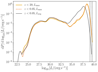
Figure 1: Distributions of the maximum X-ray luminosity $L_{\mathrm{max}}$ reached by all HMXBs in the $z_{<20}$ (solid gold line) and $z_{<0.05}$ (dashed red line) populations, along with the time-averaged X-ray luminosity $L_{\mathrm{avg}}$ of binaries during the XRB phase for the $z_{<0.05}$ population (solid black line). The left and right vertical dotted lines mark the Eddington luminosity limits for $10M_{\odot}$ and $30M_{\odot}$ BH accretors, respectively.

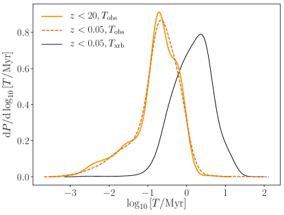
Figure 2: Distributions of the duration of detectable X-ray emission $T_{\mathrm{obs}}$ for all HMXBs in the $z_{<20}$ (solid gold line) and $z_{<0.05}$ (dashed red line) populations that emit above the minimum X-ray detection threshold for a nonzero period of time. For the $z_{<0.05}$ population, we also show the total duration of the XRB phase $T_{\mathrm{xrb}}$ (solid black line). This distribution is nearly identical to that for the $z_{<20}$ population.

3.2 Comparing Selection Effects

Here we compare the detectable HMXB and detectable merging BBH populations in order to understand the existing observational discrepancies between BHs detected in X-ray versus GW sources. Namely, we investigate the lack of observed HMXBs that are predicted to become BBH mergers, as well as the lack of high-mass BHs found in HMXBs. We use Eq. (20) and Eq. (22) to calculate detectability weights for HMXBs ($\mathcal{W}_{\mathrm{xrb}}$) and GWs ($\mathcal{W}_{\mathrm{gw}}$), respectively.

In all of these comparisons, we use the $z_{<0.05}$ HMXB population and the $z_{<20}$ BBH population. This is because the effective sample size of detectable HMXBs in the $z_{<0.05}$ population is $\simeq 50$ times larger, and thus allows for more robust statistics. The detectable HMXBs in both populations have comparable properties (in addition to the emission properties in Figure 1 and Figure 2, their redshift, metallicity, and mass distributions are consistent). We find that more than $99.9\%$ of all HMXBs in the $z_{<20}$ sample are too distant to be observed, even if they achieve high luminosities. In addition, the maximum ZAMS formation redshift of detectable HMXBs in our $z_{<0.05}$ sample is $\simeq 8\times 10^{-3}$, which is much smaller than the upper sampling bound of $z=0.05$. Thus, even if we sampled a $z_{<20}$ population with one billion systems, we still would not find any detectable HMXBs beyond $z\sim 0.01$.

3.2.1 Redshifts and Metallicities

In Figure 3, we compare the redshift distributions of HMXBs formed by today (HMXB_z0) and BBHs merged by today (BBHm_z0), weighted by their respective detectability In Figure 4, we do the same for the metallicity distributions. As expected, the progenitors of detectable HMXBs form at very low redshifts ($z_{\mathrm{f}}\lesssim 0.01$), whereas the progenitors of detectable BBHs mergers form at much higher redshifts ($z_{\mathrm{f}}\gtrsim 1$), leading to detectable BBH mergers in the redshift range $0.01\lesssim z_{\mathrm{m}}\lesssim 1$.

As a consequence of the differing redshift distributions of detectable HMXB and BBH-merger progenitors, there are also differences in the population metallicities, with the detection-weighted HMXBs having higher typical metallicities than the merging BBHs. The metallicity distribution of detectable HMXBs peaks near $0.5Z/Z_{\odot}$ while that for detectable merging BBHs peaks near $0.08Z/Z_{\odot}$. There is almost no support for detectable HMXB formation below $0.1Z/Z_{\odot}$, as fewer than $0.05\%$ of detectable HMXBs have metallicities below this limit. This is expected because the distance at which GW detectors are sensitive to merging BBHs is much larger than the distance to which we can observe HMXBs, and thus GWs probe higher redshifts and lower metallicites.

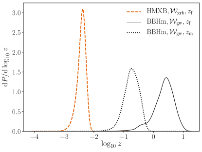
Figure 3: Distributions of the ZAMS formation redshifts $z_{\mathrm{f}}$ for $z_{<0.05}$ HMXB and $z_{<20}$ merging BBH progenitors, as well as the merger redshifts $z_{\mathrm{m}}$ for $z_{<20}$ merging BBHs, weighted by their X-ray and GW detectability, respectively.

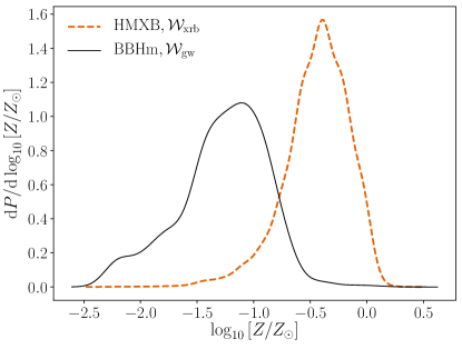
Figure 4: Distributions of progenitor metallicities for $z_{<0.05}$ HMXBs and $z_{<20}$ merging BBHs, weighted by their X-ray and GW detectability, respectively.

3.2.2 Binary Component Masses

Next, we examine the mass distributions of the $z_{<0.05}$ HMXB and $z_{<20}$ merging BBH populations. In Figure 5, we show distributions of the binary component masses at the beginning of the HMXB phase for all $z_{<0.05}$ HMXBs formed by today (HMXB_z0) and all $z_{<20}$ HMXBs that will merge as BBHs by today (BBHm_z0). The horizontal axis shows the BH accretor mass, $M_{\mathrm{BH}}/M_{\odot}$, and the vertical axis shows the donor star mass, $M_{\mathrm{donor}}/M_{\odot}$, at the start of the HMXB phase. In the top panel of Figure 5, we show the underlying mass distributions for the HMXB_z0 and BBHm_z0 populations. While the distributions mostly overlap, the BBHm_z0 distribution is centered at lower BH masses ($<20M_{\odot}$) because the majority ($\sim 70$%) of HMXBs with high-mass BH accretors form BBH systems with long delay times that do not merge by $z=0$. Finding BHs with longer delay times at higher redshifts could be an artifact of various population synthesis prescriptions for binary evolution, such as those for BH kicks, common-envelope evolution, mass transfer, etc. (e.g., van Son et al., 2022b). However, because we are only interested in obtaining a fiducial model for binary evolution in this paper, we do not investigate these effects in detail.

In the central panel of Figure 5, we show the same distributions weighted by their respective selection effects. We weight the HMXB_z0 population by their X-ray detection weights $\mathcal{W}_{\mathrm{xrb}}$ and the BBHm_z0 population by their GW detection weights $\mathcal{W}_{\mathrm{gw}}$, defined in Eq. (20) and Eq. (22), respectively. While the distributions still overlap, the detectable BBHm_z0 distribution is pulled to higher masses ($>20M_{\odot}$), which is the result of heavier BH mergers having higher GW detection probabilities. The detectable HMXB_z0 distribution remains at masses similar to the underlying distribution, as we do not find a strong correlation of $\mathcal{W}_{\mathrm{xrb}}$ with BH or donor mass. If all HMXBs were emitting at the same distance for the exact same duration and had Eddington-limited accretion, the HMXB detectability would scale with the mass of the BH accretor according to Eq. (4) through Eq. (6). However, since we do not find a discernible correlation between BH mass and detectability, it is clear that the duration of detectable emission plays a critical role in the detectability of HMXBs.

There are very few detectable HMXBs that have BH accretor masses $>35M_{\odot}$, while there is significant support for these massive systems in the GW population: fewer than $3\%$ of detectable HMXBs host BHs $>35M_{\odot}$, while $\simeq 20\%$ of detectable merging BBH progenitors have primary BH masses that exceed this limit. However, there is significant overlap between the BH masses in the detectable HMXB and detectable BBH below $35~{}M_{\odot}$. This falls in accordance with observations: the BH mass distribution inferred from GW observations peaks near $10~{}M_{\odot}$ (Abbott et al., 2022b), and all observed HMXBs have BH accretors with masses well below $35~{}M_{\odot}$.

In the bottom panel of Figure 5, we plot the same HMXB_z0 distribution along with the subpopulation of $z_{<0.05}$ HMXBs that will form merging BBHs within a Hubble time of ZAMS (BBHm_H). Here, the distributions are both weighted by their X-ray detectability. This compares the full detectable population of HMXBs to the subpopulation that will become merging BBHs within a Hubble time. Changing the (black) distribution of the BBH sample from $z_{<20}$ in the central panel to $z_{<0.05}$ in the bottom panel creates extra support for low-mass BBH mergers that is independent of changing the weights from $\mathcal{W}_{\mathrm{gw}}$ to $\mathcal{W}_{\mathrm{xrb}}$. This spread to lower masses is a result of the $z_{<0.05}$ population residing at higher metallicities.

We find that the X-ray detection-weighted BBHm_H progenitors have higher donor masses relative to the full detection-weighted HMXB population. This is because detectable HMXBs are unlikely to form BBHs in our sample; in addition to the progenitors of these stars having lower ZAMS masses, we find that many lose additional mass during the HMXB phase, making it more likely that they will ultimately form a NS or WD. In fact, only $\simeq 20\%$ of HMXBs that emit above the X-ray detection threshold for $1~{}\mathrm{Myr}$ or longer (the upper tail of the emission distribution in Figure 2) contain donor stars that will form BHs. Of these HMXBs that emit for longer times and form BBHs, over $80\%$ are too wide to merge within a Hubble time.

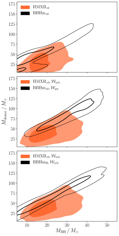
Figure 5: Distributions of HMXB component masses at the start of the XRB phase, weighted by different detector selection effects. We plot the $50\%$ and $90\%$ probability levels. The top panel shows the HMXB component masses for the full underlying $z_{<0.05}$ HMXB population (HMXB_z0) and the subpopulation of $z_{<20}$ HMXBs that will form merging BBHs by $z=0$ (BBHm_z0). The central panel shows these populations weighted by X-ray detector ($\mathcal{W}_{\mathrm{xrb}}$) and GW detector ($\mathcal{W}_{\mathrm{gw}}$) selection effects. The bottom panel shows the same HMXB_z0 population compared with the supopulation of $z_{<0.05}$ HMXBs that will form merging BBHs within a Hubble time (BBHm_H), both weighted by X-ray detector selection effects ($\mathcal{W}_{\mathrm{xrb}}$). Changing the BBH sample from $z_{<20}$ in the central panel to $z_{<0.05}$ in the bottom panel creates extra support for low-mass BBH mergers due to the $z_{<0.05}$ population residing at higher metallicities.

Finally, in Figure 6, we plot the component BH masses for HMXBs in the $z_{<0.05}$ sample that become merging BBHs in a Hubble time (BBHm_H) and the component BH masses for the population of BBHs in the $z_{<20}$ sample that merge by today (BBHm_z0). We weight the BBHm_H population by their X-ray detectability and the BBHm_z0 population by their GW detectability. This allows for comparison of the component BH mass distributions for detectable HMXBs that become BBHs and detectable BBH mergers. The population of HMXBs that become merging BBHs within a Hubble time of formation accounts for $<1\%$ of the full HMXB_z0 population, and the number of these systems that are detectable in X-ray is even smaller ($<0.05\%$ of the HMXB_z0 population). Consequently, we also plot the individual points for these systems, with the point size scaling with their X-ray detection weighting.

We find that the detection-weighted BH mass distributions overlap significantly. This is primarily because there are a handful of HMXBs with large X-ray detection weights that will form high-mass BBH mergers, even though the majority of detectable HMXBs in this population form lower-mass BBHs that are unlikely to be detected using GWs. Thus, though detectable HMXBs that result in BBH mergers have lower typical masses than BBH mergers detected via GWs, it is plausible that X-ray detectors could find a high-mass BH in a detectable HMXB system that is predicted to become a BBH GW source.

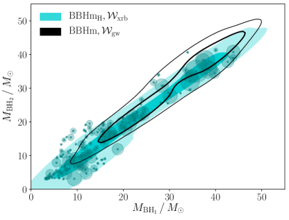
Figure 6: Distributions of the final BH component masses for the subpopulation of $z_{<0.05}$ HMXBs that will become merging BBHs in a Hubble time (BBHm_H) and the full population of $z_{<20}$ BBHs that merge by today (BBHm_z0). We plot the $50\%$ and $90\%$ probability levels. The BBHm_H distribution is weighted by X-ray detector selection effects ($\mathcal{W}_{\mathrm{xrb}}$) and the BBHm_z0 distribution is weighted by GW detector selection effects ($\mathcal{W}_{\mathrm{gw}}$). As the number of HMXBs with $\mathcal{W}_{\mathrm{xrb}}>0$ that become BBHm_H in our population is small, we plot the points for individual systems, with the point size scaling with $\mathcal{W}_{\mathrm{xrb}}$.

3.2.3 Population Probability Results

Table 1: Probabilities of obtaining various sources in our sampled populations as calculated using the methods described in Section 2.5. Here, $P(\mathrm{HMXB}_{\mathrm{obs}}|\mathrm{HMXB}_{z0})$ is the probability of detecting an HMXB in our sample; $P(\mathrm{BBHm}_{\mathrm{obs}}|\mathrm{BBHm}_{T})$ is the probability of detecting a merging BBH in our sample within an observing window of $T=100~{}\mathrm{yr}$; $P(\mathrm{BBHm}_{\mathrm{H}}|\mathrm{HMXB}_{\mathrm{obs}})$ is the probability that a detectable HMXB becomes a merging BBH within a Hubble time of formation, and $P(\mathrm{HMXB}_{\mathrm{obs}}|\mathrm{BBHm}_{\mathrm{H}})$ is the probability that a BBH that merges within a Hubble time of formation underwent a detectable HMXB phase in the past.

Probability	Approximate Value
$P(\mathrm{HMXB}_{\mathrm{obs}}|\mathrm{HMXB}_{z0})$	$2.6\times 10^{-6}$
$P(\mathrm{BBHm}_{\mathrm{obs}}|\mathrm{BBHm}_{T})$	$4.8\times 10^{-3}$
$P(\mathrm{BBHm}_{\mathrm{H}}|\mathrm{HMXB}_{\mathrm{obs}})$	$6.2\times 10^{-3}$
$P(\mathrm{HMXB}_{\mathrm{obs}}|\mathrm{BBHm}_{\mathrm{H}})$	$9.3\times 10^{-7}$

To further quantify our results, we calculate the probabilities of obtaining sources in our sampled populations using the method described in Section 2.5. These quantities are defined in the context of our sampled populations, which consist of binaries that have survived the first SN with primary NS or BH progenitor stars and companion stars that are $\geq 5M_{\odot}$ at first CO formation. The probability results are summarized in Table 1.

We find that the probability of detecting an HMXB in our $z_{<0.05}$ sample is $P(\mathrm{HMXB}_{\mathrm{obs}}|\mathrm{HMXB}_{z0})\simeq 2.6\times 10^{-6}$. This means that most HMXBs in our sample are not probable to be detected via their X-ray emission. We calculate the analogous probability for the merging BBH population in our $z_{<20}$ sample, and find the probability of detecting a BBH within an observing window of $T=100$ years is $P(\mathrm{BBHm}_{\mathrm{obs}}|\mathrm{BBHm}_{T})\simeq 4.8\times 10^{-3}$. Here, $\mathrm{BBHm}_{T}$ is the population of BBHs that merge within our past light cone for the observing window $T$. This population can be thought of as the BBH mergers we would detect in time $T$ if with a perfect detector ($p_{\mathrm{det}}=1$). Our result for this probability indicates that most BBHs in our sample are not detectable as GW sources, although this probability is higher than that for the detectable HMXBs. Thus, we conclude that both detectable HMXBs and detectable BBHs are rare outcomes from binaries across the Universe.

The probability that a detectable HMXB becomes a merging BBH in a Hubble time is $P(\mathrm{BBHm}_{\mathrm{H}}|\mathrm{HMXB}_{\mathrm{obs}})\simeq 6.2\times 10^{-3}$. This implies that even if we detect an HMXB, which itself is improbable, the detected binary will most probably not merge as a BBH within a Hubble time. This is consistent with predictions for the fates of Cyg X-1, LMC X-1, and Cyg X-3, as discussed in Section 1. Conversely, we calculate the probability that a BBH that merges within a Hubble time of formation underwent a detectable HMXB phase in the past. We find this to be $P(\mathrm{HMXB}_{\mathrm{obs}}|\mathrm{BBHm}_{\mathrm{H}})\simeq 9.3\times 10^{-7}$ for the $z_{<0.05}$ population. This probability is considerably smaller than $P(\mathrm{BBHm}_{\mathrm{H}}|\mathrm{HMXB}_{\mathrm{obs}})$, which indicates that for the population of $\mathrm{BBHm}_{\mathrm{H}}$, far fewer will have undergone a detectable HMXB phase compared to the amount of detectable HMXBs that will become merging BBHs within a Hubble time. This is expected, as only binaries formed at low redshifts can become detectable HMXBs. Thus, although $>97\%$ of BBH mergers experience an XRB phase during their evolution, it is unsurprising that the observed HMXBs are not the progenitors of merging BBHs.

The probability of a detectable HMXB forming a detectable BBH merger, $P(\mathrm{BBHm}_{\mathrm{obs}}|\mathrm{HMXB}_{\mathrm{obs}}$), is essentially zero. This is because the delay time between the HMXB phase and the GW merger is much longer than the observing window $T$. This probability is also highly sensitive to the choice of $T$, as one could theoretically choose a very long observing window and force this probability to be non-zero. Thus, $P(\mathrm{BBHm}_{\mathrm{obs}}|\mathrm{HMXB}_{\mathrm{obs}})$, and similarly $P(\mathrm{HMXB}_{\mathrm{obs}}|\mathrm{BBHm}_{\mathrm{obs}})$, do not have strong physical meanings, as they are largely determined by the choice of observing period.

4 Discussion

We investigate the major current discrepancies in HMXB and GW BH observations, namely the lack of observed HMXBs that are predicted to become BBH mergers as well as the lack of high-mass BHs found in XRBs, and find that X-ray and GW detector selection effects can explain them. To arrive at this conclusion, we applied X-ray and GW selection effects to simulated binaries from COSMIC and examined their impact on population parameters. Using our new probability formalism, we quantified the probability of obtaining detectable sources in our samples of binaries. We discuss the main conclusions of our study in detail in Section 4.1, and summarise caveats and areas for future work in Section 4.2.

4.1 Main Conclusions

From our population synthesis analysis, we conclude that:

1. Detectable HMXBs are not likely to host BHs $\mathbf{>35\emph{M}_{\odot}}$ relative to detectable BBH mergers. The mass distributions in the central panel of Figure 5 show that GW detection-weighted merging BBH progenitors pull to higher donor and BH masses compared to the full detectable HMXB population. This is expected because the GW detection probability increases with mass, while we find no strong correlation between mass and X-ray detectability. Fewer than $3\%$ of detectable HMXBs host BH accretors $>35M_{\odot}$, while $\simeq 20\%$ of detectable BBH mergers have primary BH masses that exceed this limit. These results indicate that GW detectors will preferentially see more binaries of higher mass than X-ray surveys.

2. It is highly unlikely that detectable HMXBs will form merging BBHs within a Hubble time. We calculate that the probability a detectable HMXB will merge as a BBH within a Hubble time is $\simeq 0.6\%$. This result is within one order of magnitude of predictions for the fates of Cyg X-1, Cyg X-3, and LMC X-1 (Section 1), even though population synthesis prescriptions for binary evolution vary between all studies (Belczynski et al., 2012, 2013; Neijssel et al., 2021). This rarity implies that the population of HMXBs that we do observe is unlikely to form merging BBHs. Since the sample size of observed HMXB sources with well-constrained binary properties is small, our results confirm that it is unsurprising none of these systems are likely to form merging BBHs.

3. X-ray and GW selection effects probe different redshifts and metallicities. The ZAMS formation redshift distributions for detectable HMXB and detectable merging BBH sources in Figure 3 show that detectable HMXBs form locally (around $13~{}\mathrm{Mpc}$, if these systems were in the Hubble flow), while detectable merging BBH sources form and merge at much farther distances. As a result, detectable HMXBs also form at higher metallicities near $0.5Z/Z_{\odot}$ while detectable BBH mergers form at lower metallicities below $0.1Z/Z_{\odot}$. This behavior is expected, as it mirrors what we see in observations: most HMXBs with well-constrained binary parameters are in the Milky Way or nearby Local Group galaxies that have typical metallicities of $0.1\lesssim Z/Z_{\odot}\lesssim 1$, whereas GW sources are detected at farther distances where there are more environments with low metallicity (e.g., Evans et al., 2010; Rosen et al., 2016; Krivonos et al., 2021; Abbott et al., 2019, 2021a, 2021b, 2022a).

The differences between the observational samples of HMXBs and GWs sources means that these measurements are complementary, each providing different probes of the evolution of massive stars and the formation of COs.

4.2 Caveats & Future Work

In performing our calculations, we made several simplifying approximations. First, we assume that the local universe is homogeneous, and we do not model individual galaxies or changes in metallicity within those galaxies. Variations in metallicity within galaxies can be significant (e.g., Williams et al., 2021; Taibi et al., 2022), having potential effects on binary stellar evolution. Our results should therefore be taken as approximate estimates for the $z_{<0.05}$ HMXB population.

We have also approximated the selection function of X-ray sources with a single flux threshold, but in reality these detected sources may not be resolvable as BH X-ray binaries (e.g., Lutovinov et al., 2013; Clavel et al., 2019). This discrepancy can be seen through the difference in redshifts between our sampled HMXB distribution in Figure 3 and those found in observations (e.g., Evans et al., 2010; Arnason et al., 2021; Krivonos et al., 2021). Most observed HMXBs with well-constrained binary parameters are ${<50~{}\mathrm{kpc}}$ away, which is significantly closer than the peak of our redshift distribution. To accurately model these sources, separate simulations of the Milky Way and local galaxies are required. However, as we do not attempt to reproduce existing observations of individual HMXBs, our results give a good sense of how selection effects play a role in detecting larger X-ray populations.

In addition, the Roche lobe filling factor may be important in determining HMXB detectability. Recent results from Hirai & Mandel (2021) show that focused accretion streams necessary for BH disk formation can only form in wind-fed binaries when the Roche lobe filling factor is $\gtrsim 0.8$. We check whether this condition for detectability affects our results by cutting our detectable HMXB population to include only wind-fed systems with Roche lobe filling factors $>0.8$. We find that these cuts do not significantly change our main qualitative conclusions, but they reduce the size of our detectable HMXB population by 95%. This reduction in population size will change the probabilities reported in Section 3.2.3, though it does not strongly alter the distributions in our plots; the HMXB redshift and metallicity distributions in Figure 3 and Figure 4 are nearly identical to those of the population cut based on Roche lobe filling factor, and the HMXB mass distributions in the top and center panels of Figure 5 shift to slightly lower masses with the cut population. Thus, if anything, incorporating this additional condition for detectability will further emphasize the differences in the detected binary populations due to selection effects.

While we sample our populations with redshift–metallicity evolution from the Illustris-TNG simulations (Nelson et al., 2021), the true distribution of $P(Z|z)$ is uncertain (e.g., Neijssel et al., 2019). For example, though sampling with a truncated log-normal distribution with a spread of $\sigma=0.5~{}\mathrm{dex}$ for $P(Z|z)$ gives similar fundamental results to sampling with our method using Illustris-TNG, using a tighter log-normal distribution with $\sigma=0.1~{}\mathrm{dex}$ significantly alters our results. We choose to sample with Illustris-TNG because this redshift–metallicity evolution is more physically motivated than simple analytic alternatives. Uncertainties in the redshift–metallicity evolution can affect GW populations by changing the initial conditions and evolutionary properties of their progenitor populations (e.g., Chruślińska, 2022). However, features in the BBH mass spectrum are relatively robust to variations in the joint redshift and metallicity evolution (van Son et al., 2022a).

Rapid population synthesis codes like COSMIC necessarily use approximate prescriptions for stellar and binary evolution. Therefore, they are known to have systematic effects on their produced binary populations (e.g., Shao & Li, 2019; Gallegos-Garcia et al., 2021; Marchant et al., 2021). Most of the shortcomings associated with these approximations can be well-addressed with state-of-the-art population synthesis codes like POSYDON (Fragos et al., 2022), which use detailed MESA simulations (Paxton et al., 2011) to model the full evolution of binary systems. Currently, such codes only cover a limited range of metallicities, and so cannot yet be used for studies such as ours. However, our analysis framework can be adapted to use updated population synthesis results as they become available.

We only examine isolated binary evolution scenarios in this project. In reality, we expect GW sources to form through a number of channels (e.g., Zevin et al., 2021), and these must be considered as well in order to fully understand GW sources. Considering additional formation channels may further differentiate the evolution of HMXB sources from BBH sources, which exemplifies the need to understand the selection effects (both in terms of source formation and detectability) unique to each of these populations.

Once we have more sophisticated population models that accurately track mass transfer and stellar structure, and once we include all potential formation channels, it will be possible to make more accurate forecasts of the diverse populations of detectable HMXBs and detectable BBHs. These predictions could then be compared to observations to jointly constrain uncertainties in the physics of these systems’ evolution. While we only consider masses in our work, including properties such as BH spin would provide further insights into the formation of HMXBs and BBHs, and how these populations are related.

As the LIGO–Virgo–KAGRA detector network prepares for its fourth observing run (Abbott et al., 2020b), new GW data will better resolve the mass distribution of BBHs. In addition, as HMXB measurements continue to improve with upcoming missions like the eROSITA survey set to complete in 2023 (Basu-Zych et al., 2020), more binaries will be detected with resolved component masses and more accurate BH mass measurements will be attained for previously observed systems. Combining GW and X-ray observations using studies like ours can help us build a more complete concordance model of binary evolution.

References

- Aasi et al. (2015) Aasi, J., Abbott, B. P., Abbott, R., et al. 2015, Classical and Quantum Gravity, 32, 074001, doi: 10.1088/0264-9381/32/7/074001
- Abbott et al. (2016a) Abbott, B., Abbott, R., Abbott, T., et al. 2016a, Physical Review Letters, 116, 061102, doi: 10.1103/PhysRevLett.116.061102
- Abbott et al. (2016b) Abbott, B. P., Abbott, R., Abbott, T. D., et al. 2016b, 818, L22, doi: 10.3847/2041-8205/818/2/L22
- Abbott et al. (2017) —. 2017, Physical Review Letters, 119, 161101, doi: 10.1103/PhysRevLett.119.161101
- Abbott et al. (2019) —. 2019, Physical Review X, 9, 031040, doi: 10.1103/PhysRevX.9.031040
- Abbott et al. (2020a) —. 2020a, The Astrophysical Journal Letters, 892, L3, doi: 10.3847/2041-8213/ab75f5
- Abbott et al. (2020b) —. 2020b, Living Reviews in Relativity, 23, 3, doi: 10.1007/s41114-020-00026-9
- Abbott et al. (2020c) Abbott, R., Abbott, T. D., Abraham, S., et al. 2020c, The Astrophysical Journal Letters, 896, L44, doi: 10.3847/2041-8213/ab960f
- Abbott et al. (2021a) Abbott, R., Abbott, T., Abraham, S., et al. 2021a, Physical Review X, 11, 021053, doi: 10.1103/PhysRevX.11.021053
- Abbott et al. (2021b) Abbott, R., Abbott, T. D., Acernese, F., et al. 2021b, arXiv:2111.03606 [astro-ph, physics:gr-qc]. http://arxiv.org/abs/2111.03606
- Abbott et al. (2021c) Abbott, R., Abbott, T. D., Abraham, S., et al. 2021c, The Astrophysical Journal Letters, 915, L5, doi: 10.3847/2041-8213/ac082e
- Abbott et al. (2022a) Abbott, R., Abbott, T. D., Acernese, F., et al. 2022a, GWTC-2.1: Deep Extended Catalog of Compact Binary Coalescences Observed by LIGO and Virgo During the First Half of the Third Observing Run, arXiv, doi: 10.48550/arXiv.2108.01045
- Abbott et al. (2022b) —. 2022b, The population of merging compact binaries inferred using gravitational waves through GWTC-3, arXiv, doi: 10.48550/arXiv.2111.03634
- Acernese et al. (2015) Acernese, F., Agathos, M., Agatsuma, K., et al. 2015, Classical and Quantum Gravity, 32, 024001, doi: 10.1088/0264-9381/32/2/024001
- Aghanim et al. (2020) Aghanim, N., Akrami, Y., Ashdown, M., et al. 2020, Astronomy and Astrophysics, 641, A6, doi: 10.1051/0004-6361/201833910
- Arnason et al. (2021) Arnason, R. M., Papei, H., Barmby, P., Bahramian, A., & Gorski, M. D. 2021, Monthly Notices of the Royal Astronomical Society, 502, 5455, doi: 10.1093/mnras/stab345
- Bardeen (1970) Bardeen, J. M. 1970, Nature, 226, 64, doi: 10.1038/226064a0
- Barrett et al. (2018) Barrett, J. W., Gaebel, S. M., Neijssel, C. J., et al. 2018, Monthly Notices of the Royal Astronomical Society, 477, 4685, doi: 10.1093/mnras/sty908
- Basu-Zych et al. (2020) Basu-Zych, A. R., Hornschemeier, A. E., Haberl, F., et al. 2020, Monthly Notices of the Royal Astronomical Society, 498, 1651, doi: 10.1093/mnras/staa2343
- Belczynski et al. (2012) Belczynski, K., Bulik, T., & Fryer, C. L. 2012, arXiv:1208.2422 [astro-ph]. http://arxiv.org/abs/1208.2422
- Belczynski et al. (2013) Belczynski, K., Bulik, T., Mandel, I., et al. 2013, The Astrophysical Journal, 764, 96, doi: 10.1088/0004-637X/764/1/96
- Belczynski et al. (2016) Belczynski, K., Holz, D. E., Bulik, T., & O’Shaughnessy, R. 2016, Nature, 534, 512, doi: 10.1038/nature18322
- Belczynski et al. (2008) Belczynski, K., Kalogera, V., Rasio, F. A., et al. 2008, The Astrophysical Journal Supplement Series, 174, 223, doi: 10.1086/521026
- Belczynski et al. (2022) Belczynski, K., Romagnolo, A., Olejak, A., et al. 2022, The Astrophysical Journal, 925, 69, doi: 10.3847/1538-4357/ac375a
- Blondin & Owen (1997) Blondin, J. M., & Owen, M. P. 1997, 121, 361. https://ui.adsabs.harvard.edu/abs/1997ASPC..121..361B
- Bolton (1972) Bolton, C. T. 1972, Nature, 235, 271, doi: 10.1038/235271b0
- Bondi & Hoyle (1944) Bondi, H., & Hoyle, F. 1944, Monthly Notices of the Royal Astronomical Society, 104, 273, doi: 10.1093/mnras/104.5.273
- Breivik et al. (2020) Breivik, K., Coughlin, S., Zevin, M., et al. 2020, The Astrophysical Journal, 898, 71, doi: 10.3847/1538-4357/ab9d85
- Broekgaarden et al. (2022) Broekgaarden, F. S., Berger, E., Stevenson, S., et al. 2022, Monthly Notices of the Royal Astronomical Society, doi: 10.1093/mnras/stac1677
- Chandra X-ray Center et al. (2021) Chandra X-ray Center, Chandra Project Science, MSFC, & Chandra IPI Teams. 2021, Chandra Cycle 24 Proposers’ Observatory Guide. https://cxc.harvard.edu/proposer/POG/
- Chen et al. (2021) Chen, H.-Y., Holz, D. E., Miller, J., et al. 2021, Classical and Quantum Gravity, 38, 055010, doi: 10.1088/1361-6382/abd594
- Chruślińska (2022) Chruślińska, M. 2022, Chemical evolution of the Universe and its consequences for gravitational-wave astrophysics, arXiv, doi: 10.48550/arXiv.2206.10622
- Claeys et al. (2014) Claeys, J. S. W., Pols, O. R., Izzard, R. G., Vink, J., & Verbunt, F. W. M. 2014, Astronomy and Astrophysics, 563, A83, doi: 10.1051/0004-6361/201322714
- Clavel et al. (2019) Clavel, M., Tomsick, J. A., Hare, J., et al. 2019, The Astrophysical Journal, 887, 32, doi: 10.3847/1538-4357/ab4b55
- Dominik et al. (2015) Dominik, M., Berti, E., O’Shaughnessy, R., et al. 2015, The Astrophysical Journal, 806, 263, doi: 10.1088/0004-637X/806/2/263
- Edelman et al. (2022) Edelman, B., Doctor, Z., Godfrey, J., & Farr, B. 2022, The Astrophysical Journal, 924, 101, doi: 10.3847/1538-4357/ac3667
- Evans et al. (2010) Evans, I. N., Primini, F. A., Glotfelty, K. J., et al. 2010, The Astrophysical Journal Supplement Series, 189, 37, doi: 10.1088/0067-0049/189/1/37
- Fabbiano (2006) Fabbiano, G. 2006, Annual Review of Astronomy and Astrophysics, 44, 323, doi: 10.1146/annurev.astro.44.051905.092519
- Finn & Chernoff (1993) Finn, L. S., & Chernoff, D. F. 1993, Physical Review D, 47, 2198, doi: 10.1103/PhysRevD.47.2198
- Fishbach et al. (2020) Fishbach, M., Farr, W. M., & Holz, D. E. 2020, The Astrophysical Journal, 891, L31, doi: 10.3847/2041-8213/ab77c9
- Fishbach et al. (2018) Fishbach, M., Holz, D. E., & Farr, W. M. 2018, The Astrophysical Journal, 863, L41, doi: 10.3847/2041-8213/aad800
- Fishbach & Kalogera (2022) Fishbach, M., & Kalogera, V. 2022, The Astrophysical Journal Letters, 929, L26, doi: 10.3847/2041-8213/ac64a5
- Fragos et al. (2022) Fragos, T., Andrews, J. J., Bavera, S. S., et al. 2022, POSYDON: A General-Purpose Population Synthesis Code with Detailed Binary-Evolution Simulations, arXiv, doi: 10.48550/arXiv.2202.05892
- Fryer et al. (2012) Fryer, C. L., Belczynski, K., Wiktorowicz, G., et al. 2012, The Astrophysical Journal, 749, 91, doi: 10.1088/0004-637X/749/1/91
- Gallegos-Garcia et al. (2021) Gallegos-Garcia, M., Berry, C. P. L., Marchant, P., & Kalogera, V. 2021, The Astrophysical Journal, 922, 110, doi: 10.3847/1538-4357/ac2610
- Gallegos-Garcia et al. (2022) Gallegos-Garcia, M., Fishbach, M., Kalogera, V., Berry, C. P. L., & Doctor, Z. 2022, Do high-spin high mass X-ray binaries contribute to the population of merging binary black holes?, arXiv, doi: 10.48550/arXiv.2207.14290
- Grevesse & Sauval (1998) Grevesse, N., & Sauval, A. J. 1998, Space Science Reviews, 85, 161, doi: 10.1023/A:1005161325181
- Haberl & Sturm (2016) Haberl, F., & Sturm, R. 2016, Astronomy & Astrophysics, 586, A81, doi: 10.1051/0004-6361/201527326
- Heuvel (2018) Heuvel, E. P. J. v. d. 2018, Proceedings of the International Astronomical Union, 14, 1, doi: 10.1017/S1743921319001315
- Hirai & Mandel (2021) Hirai, R., & Mandel, I. 2021, Publications of the Astronomical Society of Australia, 38, e056, doi: 10.1017/pasa.2021.53
- Hunter (2007) Hunter, J. D. 2007, Computing in Science & Engineering, 9, 90, doi: 10.1109/MCSE.2007.55
- Hurley et al. (2000) Hurley, J. R., Pols, O. R., & Tout, C. A. 2000, Monthly Notices of the Royal Astronomical Society, 315, 543, doi: 10.1046/j.1365-8711.2000.03426.x
- Hurley et al. (2002) Hurley, J. R., Tout, C. A., & Pols, O. R. 2002, Monthly Notices of the Royal Astronomical Society, 329, 897, doi: 10.1046/j.1365-8711.2002.05038.x
- Ivanova et al. (2013) Ivanova, N., Justham, S., Chen, X., et al. 2013, Astronomy and Astrophysics Review, 21, 59, doi: 10.1007/s00159-013-0059-2
- Kalogera & Baym (1996) Kalogera, V., & Baym, G. 1996, The Astrophysical Journal Letters, 470, L61, doi: 10.1086/310296
- Kratter (2011) Kratter, K. M. 2011, arXiv:1109.3740 [astro-ph]. http://arxiv.org/abs/1109.3740
- Kretschmar et al. (2019) Kretschmar, P., Fürst, F., Sidoli, L., et al. 2019, New Astronomy Reviews, 86, 101546, doi: 10.1016/j.newar.2020.101546
- Krivonos et al. (2012) Krivonos, R., Tsygankov, S., Lutovinov, A., et al. 2012, Astronomy and Astrophysics, 545, A27, doi: 10.1051/0004-6361/201219617
- Krivonos et al. (2021) Krivonos, R. A., Bird, A. J., Churazov, E. M., et al. 2021, New Astronomy Reviews, 92, 101612, doi: 10.1016/j.newar.2021.101612
- Kroupa (2001) Kroupa, P. 2001, Monthly Notices of the Royal Astronomical Society, 322, 231, doi: 10.1046/j.1365-8711.2001.04022.x
- Lattimer (2021) Lattimer, J. 2021, Annual Review of Nuclear and Particle Science, 71, 433, doi: 10.1146/annurev-nucl-102419-124827
- Lazzarini et al. (2018) Lazzarini, M., Hornschemeier, A. E., Williams, B. F., et al. 2018, The Astrophysical Journal, 862, 28, doi: 10.3847/1538-4357/aacb2a
- Livio & Soker (1988) Livio, M., & Soker, N. 1988, The Astrophysical Journal, 329, 764, doi: 10.1086/166419
- Lutovinov et al. (2013) Lutovinov, A. A., Revnivtsev, M. G., Tsygankov, S. S., & Krivonos, R. A. 2013, Monthly Notices of the Royal Astronomical Society, 431, 327, doi: 10.1093/mnras/stt168
- Mandel & Farmer (2018) Mandel, I., & Farmer, A. 2018, arXiv:1806.05820 [astro-ph, physics:gr-qc]. http://arxiv.org/abs/1806.05820
- Marchant et al. (2021) Marchant, P., Pappas, K. M. W., Gallegos-Garcia, M., et al. 2021, Astronomy & Astrophysics, 650, A107, doi: 10.1051/0004-6361/202039992
- Marchant et al. (2019) Marchant, P., Renzo, M., Farmer, R., et al. 2019, The Astrophysical Journal, 882, 36, doi: 10.3847/1538-4357/ab3426
- Mark et al. (1969) Mark, H., Price, R., Rodrigues, R., Seward, F. D., & Swift, C. D. 1969, The Astrophysical Journal, 155, L143, doi: 10.1086/180322
- McKinney (2010) McKinney, W. 2010, Proceedings of the 9th Python in Science Conference, 56, doi: 10.25080/Majora-92bf1922-00a
- Miller & Miller (2015) Miller, M. C., & Miller, J. M. 2015, Physics Reports, 548, 1, doi: 10.1016/j.physrep.2014.09.003
- Miller-Jones et al. (2021) Miller-Jones, J. C. A., Bahramian, A., Orosz, J. A., et al. 2021, Science, 371, 1046, doi: 10.1126/science.abb3363
- Motta et al. (2021) Motta, S. E., Rodriguez, J., Jourdain, E., et al. 2021, New Astronomy Reviews, 93, 101618, doi: 10.1016/j.newar.2021.101618
- Neijssel et al. (2021) Neijssel, C. J., Vinciguerra, S., Vigna-Gomez, A., et al. 2021, The Astrophysical Journal, 908, 118, doi: 10.3847/1538-4357/abde4a
- Neijssel et al. (2019) Neijssel, C. J., Vigna-Gómez, A., Stevenson, S., et al. 2019, Monthly Notices of the Royal Astronomical Society, 490, 3740, doi: 10.1093/mnras/stz2840
- Nelson et al. (2019) Nelson, D., Springel, V., Pillepich, A., et al. 2019, Computational Astrophysics and Cosmology, 6, 2, doi: 10.1186/s40668-019-0028-x
- Nelson et al. (2021) —. 2021, The IllustrisTNG Simulations: Public Data Release, arXiv, doi: 10.48550/arXiv.1812.05609
- Oh et al. (2018) Oh, K., Koss, M., Markwardt, C. B., et al. 2018, The Astrophysical Journal Supplement Series, 235, 4, doi: 10.3847/1538-4365/aaa7fd
- Orosz et al. (2007) Orosz, J. A., McClintock, J. E., Narayan, R., et al. 2007, Nature, 449, 872, doi: 10.1038/nature06218
- Orosz et al. (2009) Orosz, J. A., Steeghs, D., McClintock, J. E., et al. 2009, The Astrophysical Journal, 697, 573, doi: 10.1088/0004-637X/697/1/573
- Pavlinsky et al. (2021) Pavlinsky, M., Tkachenko, A., Levin, V., et al. 2021, Astronomy & Astrophysics, 650, A42, doi: 10.1051/0004-6361/202040265
- Paxton et al. (2011) Paxton, B., Bildsten, L., Dotter, A., et al. 2011, The Astrophysical Journal Supplement Series, 192, 3, doi: 10.1088/0067-0049/192/1/3
- Podsiadlowski et al. (2003) Podsiadlowski, P., Rappaport, S., & Han, Z. 2003, Monthly Notices of the Royal Astronomical Society, 341, 385, doi: 10.1046/j.1365-8711.2003.06464.x
- Predehl et al. (2021) Predehl, P., Andritschke, R., Arefiev, V., et al. 2021, Astronomy & Astrophysics, 647, A1, doi: 10.1051/0004-6361/202039313
- Ramachandran et al. (2022) Ramachandran, V., Oskinova, L. M., Hamann, W.-R., et al. 2022, Astronomy & Astrophysics, doi: 10.1051/0004-6361/202243683
- Remillard & McClintock (2006) Remillard, R. A., & McClintock, J. E. 2006, Annual Review of Astronomy and Astrophysics, 44, 49, doi: 10.1146/annurev.astro.44.051905.092532
- Rhoades & Ruffini (1974) Rhoades, C. E., & Ruffini, R. 1974, Physical Review Letters, 32, 324, doi: 10.1103/PhysRevLett.32.324
- Rice et al. (2021) Rice, J. R., Rangelov, B., Prestwich, A., et al. 2021, The Astrophysical Journal, 922, 178, doi: 10.3847/1538-4357/ac22ac
- Riley et al. (2022) Riley, J., Agrawal, P., Barrett, J. W., et al. 2022, The Astrophysical Journal Supplement Series, 258, 34, doi: 10.3847/1538-4365/ac416c
- Rosen et al. (2016) Rosen, S. R., Webb, N. A., Watson, M. G., et al. 2016, Astronomy & Astrophysics, 590, A1, doi: 10.1051/0004-6361/201526416
- Ryden (2002) Ryden, B. S. 2002, Introduction to Cosmology: Barbara Ryden, 1st edn. (San Francisco: Addison-Wesley)
- Sana et al. (2012) Sana, H., de Mink, S. E., de Koter, A., et al. 2012, Science, 337, 444, doi: 10.1126/science.1223344
- Shao & Li (2019) Shao, Y., & Li, X.-D. 2019, The Astrophysical Journal, 885, 151, doi: 10.3847/1538-4357/ab4816
- Spera et al. (2019) Spera, M., Mapelli, M., Giacobbo, N., et al. 2019, Monthly Notices of the Royal Astronomical Society, 485, 889, doi: 10.1093/mnras/stz359
- Taibi et al. (2022) Taibi, S., Battaglia, G., Leaman, R., et al. 2022, The stellar metallicity gradients of Local Group dwarf galaxies, arXiv, doi: 10.48550/arXiv.2206.08988
- Tauris & Heuvel (2003) Tauris, T. M., & Heuvel, E. v. d. 2003, arXiv:astro-ph/0303456. http://arxiv.org/abs/astro-ph/0303456
- Thorne (1997) Thorne, K. S. 1997, Gravitational Radiation – A New Window Onto the Universe, arXiv, doi: 10.48550/arXiv.gr-qc/9704042
- Tiwari & Fairhurst (2021) Tiwari, V., & Fairhurst, S. 2021, The Astrophysical Journal Letters, 913, L19, doi: 10.3847/2041-8213/abfbe7
- van der Walt et al. (2011) van der Walt, S., Colbert, S. C., & Varoquaux, G. 2011, Computing in Science & Engineering, 13, 22, doi: 10.1109/MCSE.2011.37
- van Son et al. (2022a) van Son, L. A. C., de Mink, S. E., Chruslinska, M., et al. 2022a, The locations of features in the mass distribution of merging binary black holes are robust against uncertainties in the metallicity-dependent cosmic star formation history, arXiv. http://arxiv.org/abs/2209.03385
- van Son et al. (2022b) van Son, L. A. C., de Mink, S. E., Callister, T., et al. 2022b, The Astrophysical Journal, 931, 17, doi: 10.3847/1538-4357/ac64a3
- Verbunt (1993) Verbunt, F. 1993, Annual Review of Astronomy and Astrophysics, 31, 93, doi: 10.1146/annurev.aa.31.090193.000521
- Vink & de Koter (2005) Vink, J. S., & de Koter, A. 2005, Astronomy and Astrophysics, 442, 587, doi: 10.1051/0004-6361:20052862
- Vink et al. (2001) Vink, J. S., de Koter, A., & Lamers, H. J. G. L. M. 2001, Astronomy and Astrophysics, 369, 574, doi: 10.1051/0004-6361:20010127
- Waskom (2021) Waskom, M. 2021, The Journal of Open Source Software, 6, 3021, doi: 10.21105/joss.03021
- Webster & Murdin (1972) Webster, B. L., & Murdin, P. 1972, Nature, 235, 37, doi: 10.1038/235037a0
- Williams et al. (2021) Williams, T. G., Kreckel, K., Belfiore, F., et al. 2021, Monthly Notices of the Royal Astronomical Society, 509, 1303, doi: 10.1093/mnras/stab3082
- Woosley (2017) Woosley, S. E. 2017, The Astrophysical Journal, 836, 244, doi: 10.3847/1538-4357/836/2/244
- Zdziarski et al. (2013) Zdziarski, A. A., Mikolajewska, J., & Belczynski, K. 2013, Monthly Notices of the Royal Astronomical Society: Letters, 429, L104, doi: 10.1093/mnrasl/sls035
- Zevin & Bavera (2022) Zevin, M., & Bavera, S. S. 2022, The Astrophysical Journal, 933, 86, doi: 10.3847/1538-4357/ac6f5d
- Zevin et al. (2020) Zevin, M., Spera, M., Berry, C. P. L., & Kalogera, V. 2020, The Astrophysical Journal Letters, 899, L1, doi: 10.3847/2041-8213/aba74e
- Zevin et al. (2021) Zevin, M., Bavera, S. S., Berry, C. P. L., et al. 2021, The Astrophysical Journal, 910, 152, doi: 10.3847/1538-4357/abe40e