BayesFT: Bayesian Optimization for Fault Tolerant Neural Network Architecture

Abstract

To deploy deep learning algorithms on resource-limited scenarios, an emerging device-resistive random access memory (ReRAM) has been regarded as promising via analog computing. However, the practicability of ReRAM is primarily limited due to the weight drifting of ReRAM neural networks due to multi-factor reasons, including manufacturing, thermal noises, and etc. In this paper, we propose a novel Bayesian optimization method for fault tolerant neural network architecture (BayesFT). For neural architecture search space design, instead of conducting neural architecture search on the whole feasible neural architecture search space, we first systematically explore the weight drifting tolerance of different neural network components, such as dropout, normalization, number of layers, and activation functions in which dropout is found to be able to improve the neural network robustness to weight drifting. Based on our analysis, we propose an efficient search space by only searching for dropout rates for each layer. Then, we use Bayesian optimization to search for the optimal neural architecture robust to weight drifting. Empirical experiments demonstrate that our algorithmic framework has outperformed the state-of-the-art methods by up to 10 times on various tasks, such as image classification and object detection.

I Introduction

Deep learning has achieved tremendous success in various fields, such as image classification, objection detection, natural language processing, and autonomous driving. To deploy deep learning algorithms on resource limited scenarios, such as internet of things, a lot of research has been conducted on integrating deep learning algorithms into deep neural network (DNN) accelerators, such as FPGAs, and domain specific ASICs. Whereas these approaches have demonstrated energy, latency and throughout efficiency improvements over traditional ways of using a general-purpose graphic computing unit (GPU), one inherent limitation is that digital circuits consume a lot of power to maintain high enough triggering voltage to differentiate two states. Besides, unlike human brains where neurons are all capable of computation and storage, information has to be transmitted repeatedly between computing component and memory to update DNNs. These properties are fundamentally different from human brains and lead to high energy costs and arguably deviating our DNN systems from emulating human intelligence.

To build machines like humans, neuromorphic computing has been proposed to simulate the human brain circuits for deep learning, which receives wide attention both from academia and industry. One emerging trend in neuromorphic computing is resistive random access memory (ReRAM) for deep learning with memristors [1, 2, 3]. Memristor is a non-volatile electronic memory device and one of the four fundamental electronic circuit components taking decades to be realized.

However, ReRAM has been demonstrated to be not well compatible with existing deep learning paradigms designed for deterministic circuit behaviors. Due to the analog property of ReRAM, the stability of ReRAM can be largely affected by thermal noises, electrical noises, process variations, and programming errors. The weights of DNN represented by the memristance of a memristor cell, can be easily distorted, largely jeopardizing the utility of the ReRAM deep learning systems.

To mitigate the negative effects of memristance distortion, several methods have been proposed whereas most of the settings are at the cost of extra hardware costs. For example, Liu et al. first learned the importance of neural network weights and then finetuned the important weights that were distorted [4]. Chen et al. proposed a method to re-write DNN into ReRAM after diagnosis for each ReRAM device. This approach is not scalable as re-training DNN is needed for each weight distortion pattern of ReRAM devices [5]. While improvements have been observed, these methods ignore factors, such as programming errors and weight drifting during usage. Besides, they are not scalable for massive production of ReRAM devices. Diagnosing and re-training DNNs for each ReRAM device are time-consuming and expensive. Recently, Liu et al. mitigated this problem with a new DNN architecture by substituting the error correction code scheme of the commonly-used softmax layer for outputting the prediction for image classification tasks [6]. In this approach, instead of predicting each class’s probability in image classification, it computed a series of binary codes from images and predicted the image’s class by comparing the series of codes with each class’s codes precomputed and stored in a codebook. For example, if for an image, the computed code is 10001, and in the codebook, the class cat’s code is 10000 and the dog’s code is 11111. As the computed code has a smaller hamming distance to the class cat’s code, the neural network will output cat as the result. Although this method does not need re-training DNNs each time, in this scheme, the errors caused by the previous layer’s weight drifts will propagate to later layers, leading to high error entanglement in the last layers responsible for generating codes. Besides, the error-correction scheme is designed for image classification tasks cannot be directly implemented in object detection tasks that are crucial in many applications, such as autonomous driving.

In this paper, we revisited the problem of fault tolerance of neural networks and identified several factors that are crucial to the robustness to weight drifting. Perhaps surprisingly, we found that the architectural choice (i.e. dropout, normalization, and complexity of models, etc) played an essential role in determining the robustness to weight drifting. We proposed a Bayesian optimization method to automatically search for fault tolerant neural network architectures. We name this approach “BayesFT”.

Our contributions can be summarized as follows:

1. We systematically analyzed the weight drifting robustness of different neural architecture components. We identified key architectural factors in determining the weight drifting robustness, such as dropout, normalization, and complexity of models.

2. Based on our analysis, we proposed a Bayesian optimization framework—BayesFT to automatically search for the fault tolerant neural network architectures that are robust to weight drifting in ReRAM devices.

3. We conducted extensive numerical experiments on various tasks and datasets, such as CIFAR-10, traffic sign recognition for image classification and PennFudanPed for object detection. Results demonstrated that our methods could improve robustness by more than 10-100 times with only negligible computational costs and engineering efforts.

II Preliminary

II-A Basics of DNN

A DNN can be viewed as the composition of many non-linear functions. Formally, given input data $\mathbf{x}\in\mathcal{R}^{d}$ and its corresponding label $\mathbf{y}$, the task is to minimize the loss $\ell(f_{\boldsymbol{\theta}}(\mathbf{x}),\mathbf{y})$, where $\ell$ is the loss function, $f$ is the neural network with weights $\mathbf{w}$. For a $K$ layer neural network, $f$ can be viewed as the composite of a series of functions $f=f_{1}\circ f_{2}\circ\cdots\circ f_{K}$. There are several commonly used layers in DNN. Convolutional layers extract features with convolution operation based on learned kernels. Fully connected layers apply non-linear function after matrix product. For more detailed introductions, we refer readers to the deep learning book [7].

II-B Memristance drifting modeling

Following the setting of [6] and [5], to simulate the memristance drifting due to multi factors as mentioned above, we apply the following drifting term to each neural network weight $w$:

$$\theta^{\prime}\leftarrow\theta e^{\lambda},\quad\lambda\sim\mathcal{N}(0,\sigma^{2})$$ (1)

where $\theta^{\prime}$ is the drifted neural network parameters, which follows a log-normal distribution. We can vary $\sigma$ to change the level of variation to simulate different ReRAM devices and deployment scenarios. It is worth noting that although we consider this setting in our paper, our methodology can be seamlessly extended to other possible weight drifting distributions.

The weight drifting in ReRAM can cause significant performance degradation for DNNs. To visualize this, a plotting of simple binary classification dataset generated with Scikit-Learn is presented. As the level of weight perturbation increases, the shape of the decision boundary shifts and therefore reduces the accuracy of classification. These figures give the intuition that the weight perturbation would cause reduction in classification accuracy.

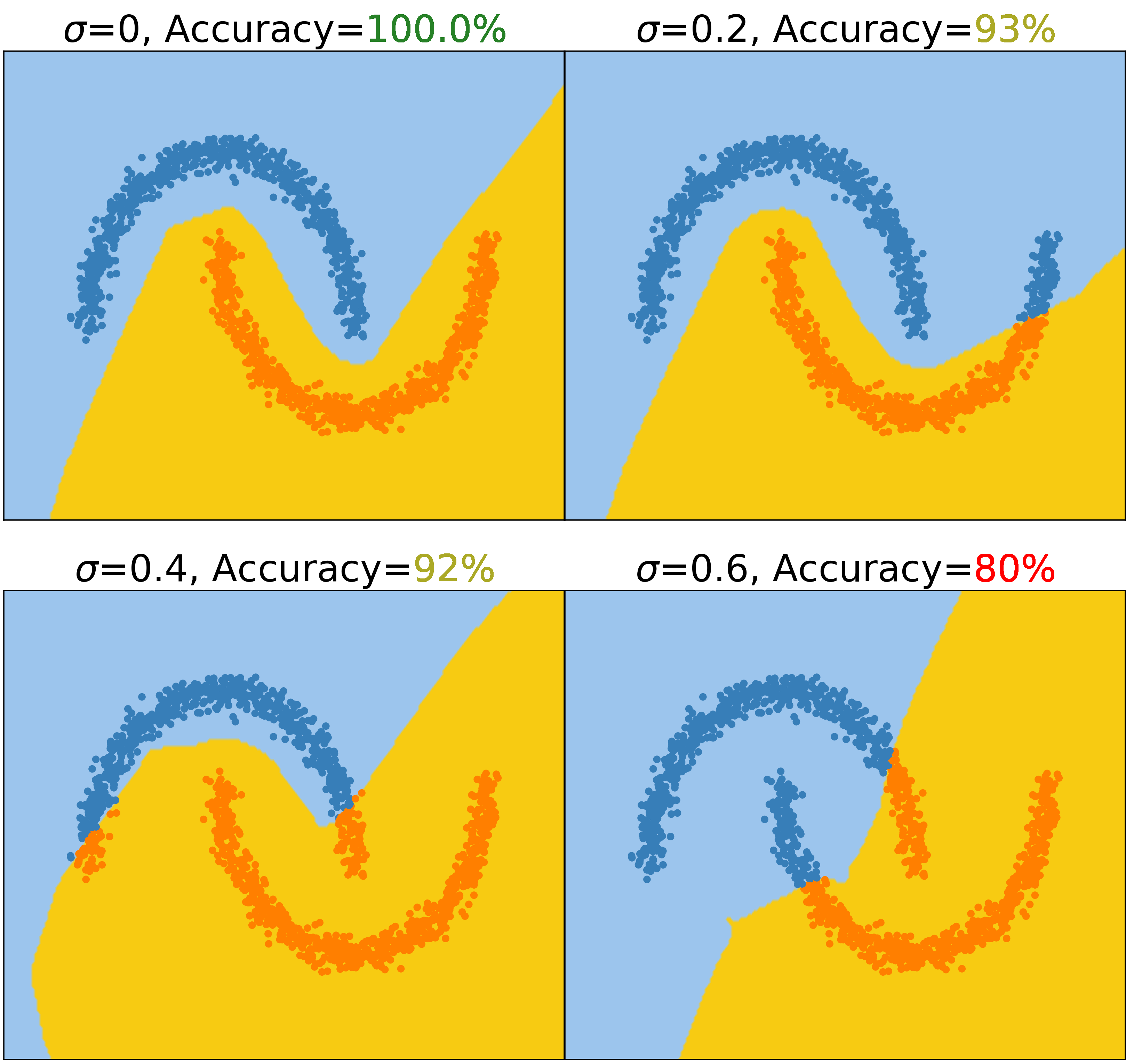
Figure 1: Decision boundary shifts caused by memristance drifting

III BayesFT: Bayesian Optimization for Fault Tolerant Neural Network Architecture

III-A Exploration of fault tolerant neural architecture

We first do an ablation study to investigate the fault tolerance of neural architecture factors, such as dropout, normalization, model complexity, and activation function using a multi-layer perceptron (MLP) on MNIST dataset. The results are shown in Figure 2. Next, we will discuss the experiment results in detail.

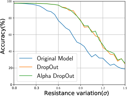
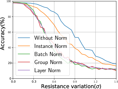
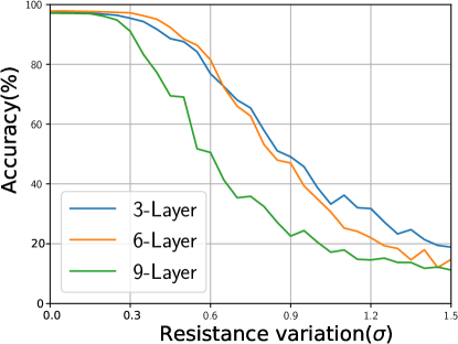
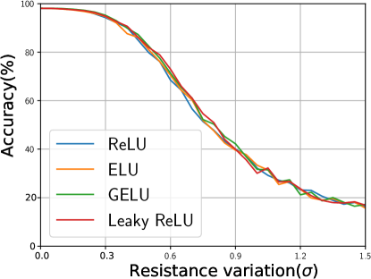
(a) Dropout (*)	(b) Normalization (*)	(c) Model complexity (*)	(d) Activation functions

Figure 2: Exploration of neural network architecture factors for fault tolerance. (*) indicates there are significant differences between methods.

Dropout

Dropout layers randomly remove neurons with a probability, often referred to as the dropout rate, which has proven effective in mitigating over-fitting in machine learning research [8]. More formally, given a weight matrix $\boldsymbol{\theta}$, the dropout layer applies a binomial distribution $\mathbf{I}\sim\text{Bernoulli}(p)$: $\boldsymbol{\theta}\leftarrow\boldsymbol{\theta}\mathbf{I}$, where $p$ is the dropout rate. We also explore a variant of dropout—alpha dropout [9]. Perhaps surprisingly, Figure 2(a) reveals that dropout layers significantly improve the robustness of network to memristance drifting. The network with dropout layer could gain self-healing ability while randomly removing weights during training process. The enhanced robustness to missing weights transfers to robustness to weight drifting. The performance of original dropout and alpha dropout are similar. The alpha dropout maintains the original input mean and variance by re-scaling after dropout. The re-scaling increases computational cost without improving the performance significantly compared to original dropout. We thus focus on the dropout for later studies.

Normalization

We considered different normalization methods commonly used in machine learning, i.e. batch normalization [10], layer normalization [11], instance normalization [12], and group normalization [13]. Each normalization method normalizes across some dimension of input features. Normalization methods empirically facilitate the convergence of optimization algorithms in machine learning.

For this family of feature normalisation methods, we perform the following computation:

$$\hat{x}_{i}=\beta\dfrac{x_{i}-\mu_{i}}{\sigma_{i}}+\gamma$$ (2)

For $\hat{x}$, the features computed by a layer, $\mu_{i}$ and $\sigma_{i}$ are mean and variance over the set $\mathcal{S}_{i}$ respectively. $i$ is the index, e.g. for 2D images $i=(i_{N},i_{C},i_{H},i_{W})$ is a 4D vector representing the features in $(N,C,H,W)$ order, where $N$ is the batch axis, $C$ is the channel axis, $H,W$ are the spatial height and width axis. $\beta$ and $\gamma$ are parameters to be trained in normalization layers. From Figure 2(b), adding normalization generally worsens the performance. This is because normalizing the hidden layer’s input to have zero mean and unit variance and then being linearly transformed creates “Achilles’s heel” as weight drifting on transformation parameter $\beta$ and $\gamma$ can be more harmful because of the normalization.

Model complexity

We tested whether more complex models or deeper DNNs can improve robustness. As shown in Figure  2(c), increasing model complexity i.e. number of layers can decrease performance. This is because drifted weights accumulate errors as the layer goes deeper. This indicates that naively applying neural architecture search (NAS) method can lead to sub-optimal performance as most NAS search spaces are built on larger models for accuracy.

Activation Function

The robustness of networks with ReLU activation function, leaky ReLU, ELU and GELU[14] is also explored. From Figure  2(c), there are no statistical differences between these methods.

III-B Bayesian optimization for fault tolerant neural network architecture

From the above analysis, we found that adding dropout layers can improve the neural network’s robustness to weight drifting significantly. However, misspecification of dropout layers can also lead to suboptimal performances. To automatically search for the optimal neural network architecture robust to weight drifting. To simplify the neural architecture search, instead of searching for all possible topology structures of DNNs, we append dropout layers after each DNN layer except the last softmax layer for output and search for the dropout rate of each layer only. We denote the specification of neural network architecture as $\boldsymbol{\alpha}\in\mathcal{R}^{K-1}$, where $K$ is the number of layers of DNNs for architectural selection. In addition to its simplicity, this neural architecture search space design is also compatible with all existing neural network architectures. This makes our method suitable for integrating into many platforms where not all neural network architectures are supported. As there is no exact gradient information available for $\boldsymbol{\alpha}$, we consider Bayesian optimization to search for the optimal $\boldsymbol{\alpha}$ from the search space [15].

We first define our objective function by marginalizing the loss over the distribution of drifting neural network parameters $\boldsymbol{\theta}$:

$$u(\boldsymbol{\alpha},\boldsymbol{\theta}) =-\mathbb{E}_{\tilde{\boldsymbol{\theta}}\sim p(\tilde{\boldsymbol{\theta}})}[\ell(f_{(\boldsymbol{\alpha},\tilde{\boldsymbol{\theta}})}(\mathbf{x}),\mathbf{y})]$$ (3)

where $\tilde{\boldsymbol{\theta}}=\boldsymbol{\theta}\exp^{\lambda}$ ,$\lambda\sim\mathcal{N}(0,\sigma^{2})$, $\ell(f_{(\boldsymbol{\alpha},\tilde{\boldsymbol{\theta}})}(\mathbf{x}),\mathbf{y})$ is the loss of a neural network with architecture $\boldsymbol{\alpha}$ and parameter $\boldsymbol{\theta}$ given input data $\mathbf{x}$ and target $\mathbf{y}$. This intractable equation can be approximately computed by Monte Carlo sampling:

$$u(\boldsymbol{\alpha},\boldsymbol{\theta}) \simeq-\frac{1}{T}\sum_{t=1}^{T}\ell(f_{(\boldsymbol{\alpha},\tilde{\boldsymbol{\theta}}_{t})}(\mathbf{x}),\mathbf{y})]$$ (4)

where $T$ is the number of Monte Carlo samples and $\tilde{\boldsymbol{\theta}}_{t}$ is the $t$-th sample randomly drawn from $p(\tilde{\boldsymbol{\theta}})$. For maximizing the objective function, we use an optimization scheme where $\boldsymbol{\alpha}$ and $\boldsymbol{\theta}$ are optimized alternatively. When optimizing $\boldsymbol{\alpha}$, we use Bayesian optimization as the gradient for $\boldsymbol{\alpha}$ is not available. Bayesian optimization uses a surrogate model constructed from previous trials to determine the point for next trial,i.e. the point which is the most likely to give the optimal solution for the gradient-free optimization problem [16]. For $\boldsymbol{\theta}$, we use the stochastic gradient descent method.

For Bayesian optimization, we use a Gaussian process regression model as the surrogate model. Suppose we already have $n$ trials of different settings of $\boldsymbol{\alpha}$ denoted as $\boldsymbol{\alpha}_{1:n}$, its corresponding objective function value $g(\boldsymbol{\alpha}_{1:n})$, and kernel matrix $\kappa(\boldsymbol{\alpha}_{1:n},\boldsymbol{\alpha}_{1:n})$, more specifically:

$$\boldsymbol{\alpha}_{1:n} =[\boldsymbol{\alpha}_{1},\cdots,\boldsymbol{\alpha}_{n}]$$ (5)

$$g(\boldsymbol{\alpha}_{1:n}) =\begin{bmatrix}u(\boldsymbol{\alpha}_{1},\boldsymbol{\theta}),&\cdots,&u(\boldsymbol{\alpha}_{n},\boldsymbol{\theta})\end{bmatrix}$$ (6)

$$\kappa(\boldsymbol{\alpha}_{1:n},\boldsymbol{\alpha}_{1:n}) =\begin{bmatrix}\kappa(\boldsymbol{\alpha}_{1},\boldsymbol{\alpha}_{1}),&\cdots,&\kappa(\boldsymbol{\alpha}_{1},\boldsymbol{\alpha}_{n})\\ \cdots,&\cdots,&\cdots\\ \kappa(\boldsymbol{\alpha}_{n},\boldsymbol{\alpha}_{1}),&\cdots,&\kappa(\boldsymbol{\alpha}_{n},\boldsymbol{\alpha}_{n})\end{bmatrix}$$ (7)

Then, according to Gaussian process’s property, the posterior probability of $g(\boldsymbol{\alpha})$ after $n$ trials follows a Gaussian distribution:

$$p(g(\boldsymbol{\alpha})|g(\boldsymbol{\alpha}_{1:n}))\sim\mathcal{N}\left(\mu_{n}(\boldsymbol{\alpha}),\sigma^{2}_{n}(\boldsymbol{\alpha})\right)$$ (8)

$$\kappa_{n}(\boldsymbol{\alpha})=\kappa(\boldsymbol{\alpha},\boldsymbol{\alpha}_{1:n})\kappa(\boldsymbol{\alpha}_{1:n},\boldsymbol{\alpha}_{1:n})^{-1}g(\alpha_{1:n})$$

$$\sigma^{2}_{n}(\boldsymbol{\alpha})=\kappa(\boldsymbol{\alpha},\boldsymbol{\alpha})-\kappa(\boldsymbol{\alpha},\boldsymbol{\alpha}_{1:n})\kappa(\boldsymbol{\alpha}_{1:n},\boldsymbol{\alpha}_{1:n})^{-1}\kappa(\boldsymbol{\alpha}_{1:n},\boldsymbol{\alpha})$$

where $\kappa$ is the kernel function. In our experiment, we use the exponential kernel function:

$$\kappa(\boldsymbol{\alpha}_{1},\boldsymbol{\alpha}_{2})=k_{0}\exp(-||\boldsymbol{\alpha}_{1}-\boldsymbol{\alpha}_{2}||^{2})$$ (9)

where $||\boldsymbol{\alpha}_{1}-\boldsymbol{\alpha}_{2}||^{2}=\sum_{i=1}^{d}k_{i}(\alpha_{1,i}-\alpha_{2,i})^{2}$, and $k_{0:d}$ are parameters of the kernel.

Then, the next trial is given by finding the point that is most likely to result in the optimal objective value: $\boldsymbol{\alpha}=\max_{\boldsymbol{\alpha}}p(g(\boldsymbol{\alpha})|g(\boldsymbol{\alpha}_{1:n}))$. Thus, we have the algorithm based on Bayesian optimization for fault tolerant neural network architecture as shown in Algorithm 1.

Algorithm 1 Bayesian Optimization for Fault Tolerant DNN

1:  Input: Dataset $(\mathbf{x},\mathbf{y})$, neural network parameters $\boldsymbol{\theta}$, dropout rates for each layer $\boldsymbol{\alpha}$, number of epochs for training neural networks $E$.

2:  Output: Trained neural network $\boldsymbol{\theta}$ and dropout rates for each layer $\boldsymbol{\alpha}$.

3:  Initialization: initialize $\boldsymbol{\theta}$ with Xavier random initialization [17], $\boldsymbol{\alpha}$ with a uniform distribution on $[0,1]$, number of iterations $t=0$:

4:  repeat

5:     for $e=1$ to $e=E$ do

6:        Optimize neural network parameters $\boldsymbol{\theta}$:

$$\boldsymbol{\theta}_{t}\leftarrow\boldsymbol{\theta}_{t-1}-\nabla_{\boldsymbol{\theta}}u(\alpha_{t-1},\boldsymbol{\theta}_{t-1})$$

7:     end for

8:     Update the posterior distribution function for Bayesian optimization:

$$g(\boldsymbol{\alpha}_{1:t-1})=\begin{bmatrix}u(\boldsymbol{\alpha}_{1},\boldsymbol{\theta}_{t}),\cdots,u(\boldsymbol{\alpha}_{t-1},\boldsymbol{\theta}_{t})\end{bmatrix}$$ (10)

$$\kappa_{t-1}(\boldsymbol{\alpha})=\kappa(\boldsymbol{\alpha},\boldsymbol{\alpha}_{1:t-1})\kappa(\boldsymbol{\alpha}_{1:t-1},\boldsymbol{\alpha}_{1:t-1})^{-1}g(\alpha_{1:t-1})$$

$$\sigma^{2}_{t-1}(\boldsymbol{\alpha})=\kappa(\boldsymbol{\alpha},\boldsymbol{\alpha})-\kappa(\boldsymbol{\alpha},\boldsymbol{\alpha}_{1:t-1})$$ (11)

$$\kappa(\boldsymbol{\alpha}_{1:t-1},\boldsymbol{\alpha}_{1:t-1})^{-1}\kappa(\boldsymbol{\alpha}_{1:t-1},\boldsymbol{\alpha})$$ (12)

9:     Calculate the optimal $\boldsymbol{\alpha}$ from the updated posterior distribution function for the surrogate model:

$$\boldsymbol{\alpha}_{t}\leftarrow\max_{\boldsymbol{\alpha}}p(g(\boldsymbol{\alpha})|g(\boldsymbol{\alpha}_{1:t-1}))$$

10:     $t\leftarrow t+1$

11:  until convergence;

IV Experiment results

In this section, we discuss the experimental details to evaluate our BayesFT. The first section describes the implementation tasks and details. And then, we discuss the illustrative results. For all our experiments, we used a server with Intel Xeon E5-2630 CPU and Geforce RTX 2080Ti GPUs. We used Pytorch 1.7.0 and CUDA 10.1 for implementing numerical experiments. We consider the experimental setting where neural networks are trained off-line on GPU servers and then deployed on ReRAM devices. This is arguably more realistic as diagnosing and correcting ReRAM on-line may largely increase latency and energy consumption. For comparison, we implemented the following baseline algorithms:

1. Empirical risk minimization(ERM):the baseline algorithm that only minimizes the empirical risk.

2. ReRAM-variations (ReRAM-V,[5]): ReRAM-V diagnoses the ReRAM circuits and readjusts the weights iteratively to improve the robustness to weight drifting until convergence.

3. Adversarial weight perturbations (AWP, [18]): AWP conducts adversarial training on the weight perturbations of neural networks to improve the robustness against weight shifts.

4. Fault tolerant neural network architecture (FTNA,[6]): FTNA replaced the original model’s last softmax layer with an error-correction coding scheme as discussed before.

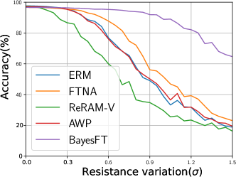
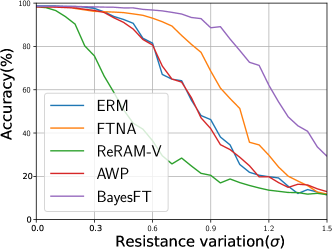
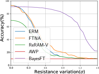
(a) MLP, Mnist	(b) LeNet, Mnist	(c) AlexNet, Cifar10	(d) ResNet-18, Cifar10	(e) VGG11, Cifar10
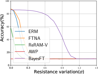
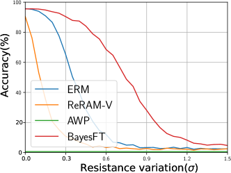
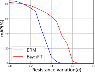
(f) PreAct-18, Cifar10	(g) PreAct-50, Cifar10	(h) PreAct-152, Cifar10	(i) MLP, GTSRB	(j) Object Detection,
				PennFudan

Figure 3: Numerical experiment results. Better viewed in the zoom-in mode.

IV-A Evaluation tasks

Image classification We consider MNIST [19], CIFAR-10 [20] , and German Traffic Sign Benchmarks (GTSRB,[21]) dataset for image classification tasks. Both MNIST and CIFAR-10 have 10 classes and GTSRB has 43 classes. For MNIST dataset, experiments were carried out on 3-layer MLP and LeNet5[22]. For CIFAR-10, we provide experimental results on commonly-used larger networks, such as ResNet[23], VGG[24], AlexNet[25], Pre-Activation-ResNet[26]. For traffic sign recognition, we used the spatial transformer network that could learn a spatial transformation to automatically transform input images for classification [27].

Object detection PennFudanPed dataset [28] was considered for object detection. The task is to detect pedestrians from input images. For this task, we used the Mask-RCNN network [29]. In this task, we found that there is no direct way to implement ReRAM-V, AWP and FTNA methods. We thus compared ERM and BayesFT.

IV-B Evaluation results

Figure 3 compares the accuracy with baseline algorithms and BayesFT across different levels of resistance variance ($0\leq\sigma\leq 1.5$) on 10 different tasks and models.

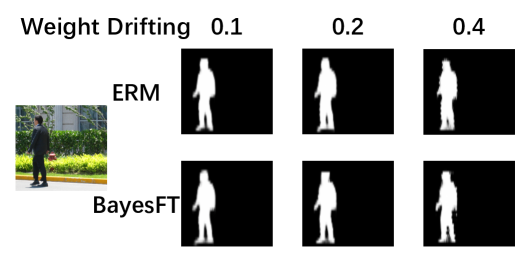
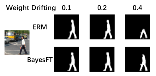
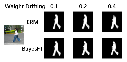
Figure 4: Visualization of object detection.

MNIST classification On MNIST dataset, all the algorithms except BayesFT experienced severe accuracy degradation as resistance variation increases. As shown in Figure 3(a), BayesFT achieved the best performance among all methods. In the small variance region ($\sigma\leq 0.6$), the MLP-MNIST remained perfectly robust with no reduction in classification accuracy. Only when $\sigma$ exceeded 0.9, the accuracy drop slightly. In contrast, the accuracy of other algorithms started to drop significantly when $\sigma$ reaches around 0.2. For larger variance ($1.2<\sigma<1.5$), BayesFT’s accuracy remained around $70\%$, making it $50\%$ more accurate than other methods. For LeNet[22] convolutional nerual network result shown in Figure 3(b), BayesFT still outperformed all the other baseline methods. For MNIST dataset, AWP had a similar performance compared to ERM, while ReRAM-V showed an unsatisfactory performance under our experimental setting. Additionally, FTNA boosted the accuracy slightly.

CIFAR-10 classification The results for CIFAR-10 classification are shown in Figure 3(c)-(g). The baseline methods’ accuracy dropped rapidly as the resistance variance increased while BayesFT could still performed stably. For example, in Figure 3(c), the accuracy of BayesFT remained almost the same for $\sigma<0.6$ and remained greater than $80\%$ for $\sigma<0.9$. It is also worth noting that in BayesFT, the accuracy drop was within $0.3\%$ when resistance variance was smaller than 0.3. Similarly, as $\sigma$ increased to 0.6 the accuracy drop was less than $2.5\%$. The improvement of accuracy gained by BayeFT is from $17\%$ to $68\%$ compared to ERM when $\sigma$ varies from $0.3$ to $0.9$. Moreover, BayesFT also demonstrated competitive results on ResNet. Figure 3(f) shows the experiment results for PreAct-18. The ERM robustness is comparably poor to AlexNet and VGG. However, applying BayesFT boosted the robustness significantly with around $50\%$ more accurate classification at variation $0.3<\sigma<1$. In addition, by comparing Figure 3(f),(g),(h), an increasingly steeper fall could be observed. This verified the conclusion we drew that the increase in depth of the neural network hurt the robustness to weight drifting. For other algorithms, the performance on CIFAR-10 dataset was not comparable to BayesFT. AWP performed the worst among all algorithms since the strong adversarial attack on the neural network parameters caused training failures.

Trafficsign classification The BayesFT method boosts performance on this 43-class and randomized input shape classification task with transformer network. ERM performs poorly on this dataset. The accuracy falls quickly and drops to around $10\%$ when $\sigma=0.6$. In contrast, with the help of BayesFT, the accuracy remains around a tolerable $70\%$. Additionally, for lower sigma variation, say $0<\sigma<0.4$, the accuracy surpasses $80\%$.

Object detection The results for object detection are shown in Figure 3(j). Compared with ERM, BayesFT largely improved the object detection accuracy—mean average precision (mAP). There is also a visualization of object detection results in Figure 4, from which we can see that ERM lost more details when weight drifting is larger. This example further shows that BayesFT can be seaminglessly applied to other tasks in addition to image classification.

V Conclusion and future work

In this paper, we proposed a novel Bayesian optimization algorithmic framework to search for fault tolerant neural architectures that are robust to memristance drifting in ReRAM DNNs. Extensive numerical experiment results demonstrate the superiority of our algorithm over other baseline methods by a large margin.

References

- [1] A. Shafiee, A. Nag, N. Muralimanohar, R. Balasubramonian, J. P. Strachan, M. Hu, R. S. Williams, and V. Srikumar, “ISAAC: A convolutional neural network accelerator with in-situ analog arithmetic in crossbars,” ACM SIGARCH Computer Architecture News, vol. 44, no. 3, pp. 14–26, 2016.
- [2] T. Liu, L. Jiang, Y. Jin, G. Quan, and W. Wen, “PT-spike: A precise-time-dependent single spike neuromorphic architecture with efficient supervised learning,” in 2018 23rd Asia and South Pacific Design Automation Conference, 2018, pp. 568–573.
- [3] P. Yao, H. Wu, B. Gao, J. Tang, and H. Qian, “Fully hardware-implemented memristor convolutional neural network,” Nature, vol. 577, no. 7792, pp. 641–646, 2020.
- [4] C. Liu, M. Hu, J. P. Strachan, and H. Li, “Rescuing memristor-based neuromorphic design with high defects,” in Design Automation Conference, 2017, pp. 1–6.
- [5] L. Chen, J. Li, Y. Chen, Q. Deng, J. Shen, X. Liang, and L. Jiang, “Accelerator-friendly neural-network training: learning variations and defects in rram crossbar,” in Proceedings of the Conference on Design, Automation & Test in Europe, 2017, pp. 19–24.
- [6] T. Liu, W. Wen, L. Jiang, Y. Wang, C. Yang, and G. Quan, “A fault-tolerant neural network architecture,” in 2019 56th ACM/IEEE Design Automation Conference, 2019, pp. 1–6.
- [7] I. Goodfellow, Y. Bengio, and A. Courville, Deep Learning. MIT Press, 2016, http://www.deeplearningbook.org.
- [8] N. Srivastava, G. Hinton, A. Krizhevsky, I. Sutskever, and R. Salakhutdinov, “Dropout: A simple way to prevent neural networks from overfitting,” Journal of Machine Learning Research, vol. 15, no. 1, pp. 1929–1958, 2014.
- [9] G. Klambauer, T. Unterthiner, A. Mayr, and S. Hochreiter, “Self-normalizing neural networks,” in Advances in Neural Information Processing Systems, 2017, pp. 971–980.
- [10] S. Ioffe and C. Szegedy, “Batch normalization: Accelerating deep network training by reducing internal covariate shift,” arXiv preprint :1502.03167, 2015.
- [11] J. L. Ba, J. R. Kiros, and G. E. Hinton, “Layer normalization,” arXiv preprint :1607.06450, 2016.
- [12] D. Ulyanov, A. Vedaldi, and V. Lempitsky, “Instance normalization: The missing ingredient for fast stylization,” arXiv preprint :1607.08022, 2016.
- [13] Y. Wu and K. He, “Group normalization,” in Proceedings of the European Conference on Computer Vision, 2018, pp. 3–19.
- [14] D. Hendrycks and K. Gimpel, “Gaussian Error Linear Units (GELUs),” arXiv preprint :1606.08415, 2016.
- [15] J. Snoek, H. Larochelle, and R. P. Adams, “Practical bayesian optimization of machine learning algorithms,” in Advances in Neural Information Processing Systems, 2012, pp. 2951–2959.
- [16] E. Brochu, V. M. Cora, and N. De Freitas, “A tutorial on bayesian optimization of expensive cost functions, with application to active user modeling and hierarchical reinforcement learning,” arXiv preprint :1012.2599, 2010.
- [17] X. Glorot and Y. Bengio, “Understanding the difficulty of training deep feedforward neural networks,” in Proceedings of the International Conference on Artificial Intelligence and Statistics (AISTATS’10). Society for Artificial Intelligence and Statistics, 2010.
- [18] D. Wu, S.-T. Xia, and Y. Wang, “Adversarial weight perturbation helps robust generalization,” Advances in Neural Information Processing Systems, vol. 33, 2020.
- [19] Y. LeCun and C. Cortes, “MNIST handwritten digit database,” 2010. [Online]. Available: http://yann.lecun.com/exdb/mnist/
- [20] A. Krizhevsky, “Learning multiple layers of features from tiny images,” Tech. Rep., 2009.
- [21] J. Stallkamp, M. Schlipsing, J. Salmen, and C. Igel, “The German Traffic Sign Recognition Benchmark: A multi-class classification competition,” in IEEE International Joint Conference on Neural Networks, 2011, pp. 1453–1460.
- [22] P. Simard, D. Steinkraus, and J. Platt, “Best practices for convolutional neural networks applied to visual document analysis,” in Seventh International Conference on Document Analysis and Recognition, vol. 2, 2003, pp. 958–958.
- [23] K. He, X. Zhang, S. Ren, and J. Sun, “Deep residual learning for image recognition,” in Proceedings of the IEEE Conference on Computer Vision and Pattern Recognition, 2016, pp. 770–778.
- [24] K. Simonyan and A. Zisserman, “Very deep convolutional networks for large-scale image recognition,” arXiv preprint :1409.1556, 2014.
- [25] A. Krizhevsky, I. Sutskever, and G. Hinton, “Imagenet classification with deep convolutional neural networks,” in Neural Information Processing Systems, 2012.
- [26] K. He, X. Zhang, S. Ren, and J. Sun, “Identity mappings in deep residual networks,” in European Conference on Computer Vision. Springer, 2016, pp. 630–645.
- [27] A. Arcos-Garcia, J. A. Alvarez-Garcia, and L. M. Soria-Morillo, “Deep neural network for traffic sign recognition systems: An analysis of spatial transformers and stochastic optimisation methods,” Neural Networks, vol. 99, pp. 158–165, 2018.
- [28] L. Wang, J. Shi, G. Song, and I.-F. Shen, “Object detection combining recognition and segmentation,” in Asian Conference on Computer Vision. Springer, 2007, pp. 189–199.
- [29] K. He, G. Gkioxari, P. Dollár, and R. Girshick, “Mask R-CNN,” in Proceedings of the IEEE international Conference on Computer Vision, 2017, pp. 2961–2969.