COARSE3D: Class-Prototypes for Contrastive Learning in Weakly-Supervised 3D Point Cloud Segmentation

Abstract

Annotation of large-scale 3D data is notoriously cumbersome and costly. As an alternative, weakly-supervised learning alleviates such a need by reducing the annotation by several order of magnitudes. We propose COARSE3D, a novel architecture-agnostic contrastive learning strategy for 3D segmentation. Since contrastive learning requires rich and diverse examples as keys and anchors, we leverage a prototype memory bank capturing class-wise global dataset information efficiently into a small number of prototypes acting as keys. An entropy-driven sampling technique then allows us to select good pixels from predictions as anchors. Experiments on three projection-based backbones show we outperform baselines on three challenging real-world outdoor datasets, working with as low as 0.001% annotations.

1 Introduction

Semantic segmentation is the holy task of any scene understanding system. For driving, this is of utmost importance, because driving requires a fine-grained 3D understanding for navigation and planning. Subsequently, in recent years, 3D semantic segmentation attracted a plethora of works [Cortinhal et al.(2020)Cortinhal, Tzelepis, and Erdal Aksoy, Hu et al.(2020)Hu, Yang, Xie, Rosa, Guo, Wang, Trigoni, and Markham, Wu et al.(2018a)Wu, Wan, Yue, and Keutzer, Zhu et al.(2021)Zhu, Zhou, Wang, Hong, Ma, Li, Li, and Lin]. However, the vast majority of the literature relies on supervised learning – thus assuming dense point-wise semantic labels – which are laborious and costly to acquire. A striking example is the popular urban dataset SemKITTI [Behley et al.(2019)Behley, Garbade, Milioto, Quenzel, Behnke, Stachniss, and Gall], which took more than 1700 hours to label by human operators.

To alleviate this cost, weakly-supervised 3D segmentation uses several orders of magnitude fewer labels [Hu et al.(2022)Hu, Yang, Fang, Guo, Leonardis, Trigoni, and Markham, Liu et al.(2021)Liu, Qi, and Fu, Wu et al.(2021)Wu, Liu, Huang, Lee, Su, Huang, and Hsu, Wei et al.(2020)Wei, Lin, Yap, Hung, and Xie]. Still, researches are mostly focused on point-based backbones which are efficient but often slow at inference. Conversely, projection-based methods [Milioto et al.(2019)Milioto, Vizzo, Behley, and Stachniss, Aksoy et al.(2020)Aksoy, Baci, and Cavdar, Cortinhal et al.(2020)Cortinhal, Tzelepis, and Erdal Aksoy, Xu et al.(2020a)Xu, Wu, Wang, Zhan, Vajda, Keutzer, and Tomizuka] were shown to operate at high speed with competitive performance [Cortinhal et al.(2020)Cortinhal, Tzelepis, and Erdal Aksoy].

In this work, we propose an architecture-agnostic contrastive learning framework for weakly-supervised semantic segmentation. Since our approach does not alter the backbone segmentation, we demonstrate its usage on a lightweight projection backbone, thus enabling both efficient trainings with extreme scarce labels and fast inference. Of paramount importance, contrastive learning needs abundant representative examples [He et al.(2020)He, Fan, Wu, Xie, and Girshick, Chen et al.(2020b)Chen, Fan, Girshick, and He, Wu et al.(2018c)Wu, Xiong, Yu, and Lin] which is non-trivial to get in weakly-supervised settings. To solve this we introduce two mechanisms. First, we propose a prototype memory bank that stores the global dataset per-class information into a small number of rich and compact prototypes. Second, we employ an entropy-driven sampling to select sufficiently good anchors from inaccurate predictions. Experiments show that our method outperform existing weakly-supervised baselines on three real-world outdoor datasets SemKITTI [Behley et al.(2019)Behley, Garbade, Milioto, Quenzel, Behnke, Stachniss, and Gall], SemPOSS [Pan et al.(2020)Pan, Gao, Mei, Geng, Li, and Zhao], and nuScenes [Caesar et al.(2020)Caesar, Bankiti, Lang, Vora, Liong, Xu, Krishnan, Pan, Baldan, and Beijbom]. On SemKITTI we also show that we on par with full-supervision (i.e., 100% labels) performance, using only 1% of the labels. Our code is released at: https://github.com/cv-rits/COARSE3D.
In brief, our contributions can be summarized as follows:

• We propose an architecture-agnostic framework for weakly-supervised 3D point cloud segmentation and, to the best of our knowledge, first, demonstrate its usage on a lightweight projection backbone.

• We introduce a prototype memory bank that captures per-class dataset information with an entropy-driven sampling technique to sample more confident pixels as anchors.

• Our strategy significantly outperforms all comparable baselines on three real-world outdoor datasets, with as few labels as 0.001% – roughly corresponding to a single labelled point per frame.

2 Related Work

Label-efficient 3D Semantic Segmentation. With the abundant annotated large-scale 3D datasets [Behley et al.(2019)Behley, Garbade, Milioto, Quenzel, Behnke, Stachniss, and Gall, Pan et al.(2020)Pan, Gao, Mei, Geng, Li, and Zhao, Caesar et al.(2020)Caesar, Bankiti, Lang, Vora, Liong, Xu, Krishnan, Pan, Baldan, and Beijbom, Liao et al.(2021)Liao, Xie, and Geiger, Dai et al.(2017)Dai, Chang, Savva, Halber, Funkhouser, and Nießner], point cloud semantic segmentation advanced rapidly. The methods can be categorized into point-based [Cheng et al.(2021)Cheng, Razani, Taghavi, Li, and Liu, Tang et al.(2020)Tang, Liu, Zhao, Lin, Lin, Wang, and Han, Rosu et al.(2020)Rosu, Schutt, Quenzel, and Behnke, Hu et al.(2020)Hu, Yang, Xie, Rosa, Guo, Wang, Trigoni, and Markham, Tatarchenko et al.(2018)Tatarchenko, Park, Koltun, and Zhou, Su et al.(2018)Su, Jampani, Sun, Maji, Kalogerakis, Yang, and Kautz, Landrieu and Simonovsky(2018)] and projection-based [Cortinhal et al.(2020)Cortinhal, Tzelepis, and Erdal Aksoy, Aksoy et al.(2020)Aksoy, Baci, and Cavdar, Xu et al.(2020a)Xu, Wu, Wang, Zhan, Vajda, Keutzer, and Tomizuka, Wu et al.(2019)Wu, Zhou, Zhao, Yue, and Keutzer, Wu et al.(2018a)Wu, Wan, Yue, and Keutzer, Milioto et al.(2019)Milioto, Vizzo, Behley, and Stachniss] approaches. To learn from fewer labels, various strategies were proposed with point-based methods: enforcing geometric prior [Xu and Lee(2020)], local neighborhood propagation [Hu et al.(2022)Hu, Yang, Fang, Guo, Leonardis, Trigoni, and Markham, Liu et al.(2021)Liu, Qi, and Fu], for smarter use of the rare labels some used active learning  [Wu et al.(2021)Wu, Liu, Huang, Lee, Su, Huang, and Hsu], pseudo labelling [Wei et al.(2020)Wei, Lin, Yap, Hung, and Xie, Li et al.(2022)Li, Xie, Shen, Ke, Qiao, Ren, Lin, and Ma, Shi et al.(2022)Shi, Wei, Li, Liu, and Lin], graph propagation [Liu et al.(2021)Liu, Qi, and Fu, Shi et al.(2022)Shi, Wei, Li, Liu, and Lin], self-training [Li et al.(2022)Li, Xie, Shen, Ke, Qiao, Ren, Lin, and Ma, Zhang et al.(2021b)Zhang, Qu, Xie, Li, Zheng, and Li], temporal matching [Shi et al.(2022)Shi, Wei, Li, Liu, and Lin, Unal et al.(2022)Unal, Dai, and Van Gool].

Contrastive Learning for 3D. Contrastive learning [Chen et al.(2020a)Chen, Kornblith, Norouzi, and Hinton, Chen et al.(2020b)Chen, Fan, Girshick, and He, He et al.(2020)He, Fan, Wu, Xie, and Girshick], initially designed for 2D, was extended to 3D using similar points from different views in [Zhang et al.(2021c)Zhang, Girdhar, Joulin, and Misra, Xie et al.(2020b)Xie, Gu, Guo, Qi, Guibas, and Litany, Hou et al.(2021)Hou, Graham, Nießner, and Xie, Lal et al.(2021)Lal, Prabhudesai, Mediratta, Harley, and Fragkiadaki]. Limited training data is considered in [Hou et al.(2021)Hou, Graham, Nießner, and Xie]. Invariant representation is learned from spatio-temporal cues in [Chen et al.(2022)Chen, Nießner, and Dai, Huang et al.(2021)Huang, Xie, Zhu, and Zhu, Liang et al.(2021)Liang, Jiang, Feng, Chen, Xu, Liang, Zhang, Li, and Van Gool]. Pairs of point and pixels regions were matched in [Sautier et al.(2022)Sautier, Puy, Gidaris, Boulch, Bursuc, and Marlet] while point-pixel pairs are regarded as a whole in [Liu et al.(2020)Liu, Yi, Zhang, Fan, Funkhouser, and Dong]. We focus the literature on crucial aspects for our work.

Sampling Strategy is crucial for constrastive learning that requires many good examples [Kaya and Bilge(2019), Chen et al.(2020b)Chen, Fan, Girshick, and He, He et al.(2020)He, Fan, Wu, Xie, and Girshick, Wu et al.(2018c)Wu, Xiong, Yu, and Lin]. Prior knowledge is used to guide sampling in [Hadsell et al.(2006)Hadsell, Chopra, and LeCun, Bell and Bala(2015)]. Multiple pairs of positive and negative data are sampled in [Bucher et al.(2016b)Bucher, Herbin, and Jurie, Sohn(2016)]. To improve convergence, hard negative sampling is exploited in [Simo-Serra et al.(2015)Simo-Serra, Trulls, Ferraz, Kokkinos, Fua, and Moreno-Noguer, Bucher et al.(2016a)Bucher, Herbin, and Jurie, Schroff et al.(2015)Schroff, Kalenichenko, and Philbin, Khosla et al.(2020)Khosla, Teterwak, Wang, Sarna, Tian, Isola, Maschinot, Liu, and Krishnan, Robinson et al.(2021)Robinson, Chuang, Sra, and Jegelka, Kalantidis et al.(2020)Kalantidis, Sariyildiz, Pion, Weinzaepfel, and Larlus] and point proxies serve as examples in [Movshovitz-Attias et al.(2017)Movshovitz-Attias, Toshev, Leung, Ioffe, and Singh]. To avoid local minima, semi-hard negative sampling is proposed in [Schroff et al.(2015)Schroff, Kalenichenko, and Philbin, Cai et al.(2020)Cai, Frankle, Schwab, and Morcos, Xie et al.(2020a)Xie, Zhan, Liu, Ong, and Loy]. In [Cui et al.(2016)Cui, Zhou, Lin, and Belongie], false positive images are used as hard negative examples. Since noisy samples were shown to deteriorate performance [Wu et al.(2017)Wu, Manmatha, Smola, and Krahenbuhl], hard positive/negative examples sampling is applied in [Khosla et al.(2020)Khosla, Teterwak, Wang, Sarna, Tian, Isola, Maschinot, Liu, and Krishnan] while high-quality anchors are sampled by considering correct prediction in [Wang et al.(2021a)Wang, Zhou, Yu, Dai, Konukoglu, and Gool]. We instead propose entropy-driven anchors sampling techniques to learn more robust representations.

Memory Bank introduced in [Wu et al.(2018c)Wu, Xiong, Yu, and Lin] allows storing many examples, e.gpixels in 2D, typically sampled per image [Xie et al.(2021)Xie, Lin, Zhang, Cao, Lin, and Hu, Wang et al.(2021b)Wang, Zhang, Shen, Kong, and Li, Chaitanya et al.(2020)Chaitanya, Erdil, Karani, and Konukoglu] or mini-batch [Wang et al.(2021a)Wang, Zhou, Yu, Dai, Konukoglu, and Gool] to increase variety. However, such storage comes at the cost of large memory and asynchronous updates. These issues are mitigated using momentum encoder [Chen et al.(2020b)Chen, Fan, Girshick, and He, He et al.(2020)He, Fan, Wu, Xie, and Girshick] or keeping examples in recent batches [Chen et al.(2020b)Chen, Fan, Girshick, and He, He et al.(2020)He, Fan, Wu, Xie, and Girshick, Wang et al.(2020)Wang, Zhang, Huang, and Scott]. Pixels are selected randomly [Wang et al.(2021a)Wang, Zhou, Yu, Dai, Konukoglu, and Gool] or selectively [Alonso et al.(2021)Alonso, Sabater, Ferstl, Montesano, and Murillo] from each image. Still, only a few pixels are stored due to memory constraints, losing full dataset content. Moreover, using pixels embeddings is redundant [Wang et al.(2021a)Wang, Zhou, Yu, Dai, Konukoglu, and Gool]. Regions [Wang et al.(2021a)Wang, Zhou, Yu, Dai, Konukoglu, and Gool, Hu et al.(2021)Hu, Cui, and Wang] can be employed as more compact representation but not with label sparsity settings due to the need of per-pixel annotation. Hence, we propose an efficient memory bank, storing prototypes (instead of pixels) that can capture the class-wise dataset-wise information using only a small number of prototypes.

Prototype Learning aims to represent the embedding space as a set of prototypes. It is used for many tasks like classification [Cover and Hart(1967), Garcia et al.(2012)Garcia, Derrac, Cano, and Herrera, Goldberger et al.(2004)Goldberger, Hinton, Roweis, and Salakhutdinov, Salakhutdinov and Hinton(2007), Guerriero et al.(2018)Guerriero, Caputo, and Mensink, Mettes et al.(2019)Mettes, van der Pol, and Snoek, Wu et al.(2018b)Wu, Efros, and Yu, Yang et al.(2018)Yang, Zhang, Yin, and Liu], few-/zero-shot [Snell et al.(2017)Snell, Swersky, and Zemel, Jetley et al.(2015)Jetley, Romera-Paredes, Jayasumana, and Torr, Bucher et al.(2016a)Bucher, Herbin, and Jurie], regression [Mettes et al.(2019)Mettes, van der Pol, and Snoek], unsupervised learning [Wu et al.(2018c)Wu, Xiong, Yu, and Lin, Xu et al.(2020b)Xu, Xian, Wang, Schiele, and Akata], explanability [Li et al.(2018)Li, Liu, Chen, and Rudin], and semantic segmentation [Zhou et al.(2022)Zhou, Wang, Konukoglu, and Van Gool, Dong and Xing(2018), Vinyals et al.(2016)Vinyals, Blundell, Lillicrap, Wierstra, et al., Wang et al.(2019)Wang, Liew, Zou, Zhou, and Feng]. Different from the literature, we use prototypes as a memory bank to gather the rich class-wise global context information from the whole dataset efficiently.

3 Proposed approached

We address the problem of 3D semantic segmentation of point clouds and propose, a novel architecture-agnostic training strategy for weakly-supervised learning coined ‘COARSE3D’. To learn efficient semantic representation from scarce labels, we leverage a custom contrastive learning module whose originality resides in a lightweight memory footprint and sparse embedding optimization. Results show our methodology is efficient with as little as $0.001\%$ of the labelled data – stepping ahead of prior works [Hu et al.(2022)Hu, Yang, Fang, Guo, Leonardis, Trigoni, and Markham, Xu and Lee(2020), Zhang et al.(2021a)Zhang, Li, Xie, Qu, Li, and Mei, Zhang et al.(2021c)Zhang, Girdhar, Joulin, and Misra].

COARSE3D, depicted in Fig. 1, uses a custom contrastive module (Sec. 3.1) that projects features of the segmenter encoder into a different embedding space. As for the segmenter backbone, we employ the fast and memory efficient SalsaNext [Cortinhal et al.(2020)Cortinhal, Tzelepis, and Erdal Aksoy] which processes 3D point cloud as 2D range images. Rather than the greedy pixel-wise memory [Wang et al.(2021a)Wang, Zhou, Yu, Dai, Konukoglu, and Gool], our projected features are clustered into a prototype memory bank (Sec. 3.2) that captures compact class-wise semantic embeddings. This enables preserving the dataset context in a significantly lighter fashion. In each iteration, we optimize only a small subset of pixels (i.e. anchors) sampled with an entropy-based strategy (Sec. 3.3) considering prototypes as positive/negative samples (i.e. keys). Our training strategy (Sec. 3.4) combines standard segmentation and contrastive losses, along with a simple labels propagation strategy.

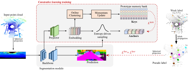
Figure 1: Our COARSE3D uses a contrastive learning strategy (Sec. 3.1) to learn high dimensional semantic embeddings from the encoder features, later clustered into a lightweight prototype memory bank (Sec. 3.2). At each step, contrastive learning is applied on a scarce set of ‘anchors’, selected from an entropy-based sampling (Sec. 3.3), which features are pushed towards (pulled away from) positive (negative) prototypes acting as ‘keys’.

3.1 Contrastive Learning Pipeline

We leverage a contrastive learning scheme since prior works have shown its effectiveness to learn from limited labels [Xie et al.(2020b)Xie, Gu, Guo, Qi, Guibas, and Litany, Rozenberszki et al.(2022)Rozenberszki, Litany, and Dai, Hou et al.(2021)Hou, Graham, Nießner, and Xie]. We build on the standard InfoNCE pixel-wise contrastive loss [Oord et al.(2018)Oord, Li, and Vinyals, Gutmann and Hyvärinen(2010)] but apply the latter between our class-wise representations, hereafter prototypes (Sec. 3.2), and a subset of sampled pixels (Sec. 3.3).

More specifically, at each training iteration we select a set of pixels, called anchors having features $\mathcal{A}{=}\{a_{j},...,a_{N_{\text{a}}}\}$. For each anchor, we select the corresponding prototypes of similar semantic class, i.e. positive keys with features $\mathcal{P}^{+}{=}\{p^{+}_{1},...,p^{+}_{N^{+}}\}$, or different semantic class, i.e. negative keys with features $\mathcal{P}^{-}{=}\{p^{-}_{1},...,p^{-}_{N^{-}}\}$. The InfoNCE optimization objective is to simultaneously pull the embedding of anchors towards positive keys while pushing them away from the negative keys. Formally, it writes:

$$\mathcal{L}^{\text{Pix2Proto}}=\frac{1}{N_{\text{a}}}\sum_{a_{i}\in\mathcal{A}}-\text{log}\frac{\sum_{p_{j}^{+}\in\mathcal{P}^{+}}\exp\left(a_{i}\cdot p_{j}^{+}/\tau\right)}{\sum_{p_{j}^{+}\in\mathcal{P}^{+}}\exp\left(a_{i}\cdot p_{j}^{+}/\tau\right)+\sum_{p_{j}^{-}\in\mathcal{P}^{-}}\exp\left(a_{i}\cdot p_{j}^{-}/\tau\right)}\,,$$ (1)

where $\tau$ is the temperature hyperparameter. All feature vectors are extracted by first linearly interpolating multi-scale features to the full image size. Then, they are concatenated and mapped to 256-dim using two $1{\times}1$ 2D convolutional layers. Finally, they are $\ell^{2}$-normalized. Following previous works [Kaya and Bilge(2019), Wang et al.(2021a)Wang, Zhou, Yu, Dai, Konukoglu, and Gool] that demonstrated the benefit of a custom selection of keys and anchors, we consider a set of anchors sampled using the entropy of the segmentation output and keys from a newly introduced prototype memory bank, that we describe next.

3.2 Prototype Memory Bank

The memory bank requires massive data to learn good representation which is traditionally achieved by storing a large number of pixels as in [He et al.(2020)He, Fan, Wu, Xie, and Girshick, Wang et al.(2021a)Wang, Zhou, Yu, Dai, Konukoglu, and Gool, Wu et al.(2018c)Wu, Xiong, Yu, and Lin, Wang et al.(2020)Wang, Zhang, Huang, and Scott]. Still, this is very costly in terms of memory and computation for contrastive sampling. Furthermore, storing pixels is semantically redundant which can be mitigated by storing semantic regions [Wang et al.(2021a)Wang, Zhou, Yu, Dai, Konukoglu, and Gool]. However, the latter would be poorly reliable given the limited labels. Therefore, we introduce a prototype memory bank that encodes class-wise embedding into compact prototypes.

More in-depth, the memory bank stores $\{P_{k}\in\mathbb{R}^{N_{p}{\times}D}\}^{K}_{k=1}$ prototypes of feature dimension $D$, corresponding to $N_{p}$ prototypes per class for each of the $K$ semantic classes. For each semantic class $k$, at each training iteration, we cluster the $N_{k}$ labelled pixels of such class into the corresponding $N_{p}$ class prototypes. We frame this as an optimal transport problem and employ the Sinkhorn algorithm [Cuturi(2013)], similar to [Zhou et al.(2022)Zhou, Wang, Konukoglu, and Van Gool] because it balances the pixels assignment between all prototypes. Here, note that the prototypes are solely updated from the embeddings of labelled pixels which guarantees reliable information.

In pratice, we compute the optimal transport matrix $T\in\mathbb{R}^{N_{k}{\times}N_{p}}$ by unrolling three iterations of the Sinkhorn algorithm on the cost matrix $\mathcal{C}\in\mathbb{R}^{N_{k}{\times}N_{p}}$ – where $\mathcal{C}_{ij}$ is the cosine distance between the feature maps of pixel $i$ and prototype $j$. The pixel-prototype mapping of pixel $p_{i}$ is obtained with $m(p_{i}){=}\text{argmax}_{j}T_{ij}$. In practice, to encourage exploration we use a Gumbel-Softmax ($\tau{=}0.5$) as differentiable argmax. Given a random initialization, we update each prototype with a $\sigma=0.999$ momentum towards the mean of the clustered pixels embeddings in each training iteration. Hence, $j^{th}$ prototype $\{P_{k}\}_{j}$ of class $k$ is updated as:

$$\{P_{k}\}_{j}=\sigma\{P_{k}\}_{j}+(1-\sigma)\frac{1}{\sum_{i=1}^{N_{k}}\llbracket m(x_{i}){=}j\rrbracket}\sum_{i=1}^{N_{k}}{x_{i}}\llbracket m(x_{i}){=}j\rrbracket\,,$$ (2)

with $\llbracket.\rrbracket$ the Iverson brackets.

3.3 Entropy-driven Anchors Sampling

Prior works have shown the importance of proper sampling in contrastive learning [Bucher et al.(2016a)Bucher, Herbin, and Jurie, Kalantidis et al.(2020)Kalantidis, Sariyildiz, Pion, Weinzaepfel, and Larlus, Sohn(2016), Cai et al.(2020)Cai, Frankle, Schwab, and Morcos, Wang et al.(2021a)Wang, Zhou, Yu, Dai, Konukoglu, and Gool, Xie et al.(2020a)Xie, Zhan, Liu, Ong, and Loy, Schroff et al.(2015)Schroff, Kalenichenko, and Philbin]. However, such strategies are inappropriate in our setup given the limited labels and the need for abundant samples in contrastive learning. Instead, we build on information theory [Shannon(2001)] and introduce an entropy-driven sampling technique to select the most appropriate pixels to serve as anchors among the abundant pseudo-labels predictions.

Given an image $x$ processed by the segmentation module, we estimate the quality of the semantic prediction for pixel $x_{i}$ using its Shannon entropy $H(x_{i})=-$ $\sum_{k=1}^{K}f(x_{i})\log(f(x_{i}))$, where $K$ is the number of classes and $f(x_{i})\in\mathcal{R}^{K}$ is the softmax prediction. Subsequently, we define the sampling probability as $\rho(x_{i})=\frac{\exp{-{H(x_{i})}^{2}}}{\sum_{x_{j}\in\mathcal{X}}\exp{-{H(x_{j})}^{2}}}$ where $\mathcal{X}$ is set of pixels with the same predicted label as $x_{i}$. Intuitively, pixels with low entropy will have higher chances to be selected. The power of $2$ is used to make the distribution steeper. Finally, we perform weighted sampling to select the $N_{a}$ pixels as a set of anchors $\mathcal{A}$. Unlike standard pixel-wise contrastive loss [Wang et al.(2021a)Wang, Zhou, Yu, Dai, Konukoglu, and Gool] requiring thousands of pixels, we start with only one anchor and linearly increase during training – up to 50% pseudo label. This follows the intuition that the segmentation module improves as training progresses.

3.4 Training Strategy

To train the method, we first apply a simple voxel propagation scheme to expand labels illustrated in Fig. 1 and detailed in Appendix B.1. We then train with two supervised and one unsupervised loss. First, the focal loss [Lin et al.(2020)Lin, Goyal, Girshick, He, and Dollár] is applied on all labelled points to alleviate classes imbalance:

$$\mathcal{L}_{i}^{\mathrm{foc}}=-\alpha(1-(f(x_{i}))^{\gamma}\log(f(x_{i}))\,,$$ (3)

where $\alpha=\{w_{k}\mid y_{i}=k\}$ is the weight of class $k$, $y_{i}$ the pseudo label of point $i$, and $w_{k}=\log(1+\frac{1}{\text{freq}_{k}})$ with $\text{freq}_{k}$ is the class frequency before voxel propagation. Second, we use the lovász-softmax loss [Berman et al.(2018)Berman, Triki, and Blaschko] to directly optimize the mean intersection-over-union, defined as:

$$\mathcal{L}_{i}^{\mathrm{lov}}=\frac{1}{k}\sum_{k=1}^{K}\overline{\Delta_{J_{k}}}(\tilde{\mathbf{m}}(c))\;\text{, with}\;\;\;\;\tilde{\mathbf{m}}_{i}(k)=\begin{cases}1-f(x_{i})&\text{ if }k=y_{i},\\ f(x_{i})&\text{ otherwise, }\end{cases}\,$$ (4)

where $\overline{\Delta_{J_{s}}}$ indicates the Lovász extension of the Jaccard index for class $k$. $y_{i}$ is the label of point $x_{i}$. Finally, the overall training target is

$$\mathcal{L}=\sum_{i}\left(\lambda_{\text{ce}}\mathcal{L}_{i}^{\mathrm{foc}}+\lambda_{\text{lov}}\mathcal{L}_{i}^{\mathrm{lov}}+\lambda_{\text{nce}}\mathcal{L}_{i}^{\mathrm{nce}}\right)\,.$$ (5)

4 Experiments

We evaluate our proposal by comparing against recent baselines on 3 challenging real-world LiDAR datasets, being SemKITTI [Behley et al.(2019)Behley, Garbade, Milioto, Quenzel, Behnke, Stachniss, and Gall], nuScenes [Caesar et al.(2020)Caesar, Bankiti, Lang, Vora, Liong, Xu, Krishnan, Pan, Baldan, and Beijbom] and SemPOSS[Pan et al.(2020)Pan, Gao, Mei, Geng, Li, and Zhao] and report main results in Sec. 4.2 and ablations in Sec. 4.3. For memory-efficient processing, we evaluate solely on projection-based backbones but COARSE3D is applicable to any architecture (e.g., point-based). In particular main results use SalsaNext [Cortinhal et al.(2020)Cortinhal, Tzelepis, and Erdal Aksoy] backbone and we experiment with Rangenet-21 [Milioto et al.(2019)Milioto, Vizzo, Behley, and Stachniss] and SqueezeSegV3-21 [Xu et al.(2020a)Xu, Wu, Wang, Zhan, Vajda, Keutzer, and Tomizuka] backbones in ablations. Importantly, all our components are removed at inference, leaving the segmenter backbone unchanged.

4.1 Experimental Setup

Datasets. SemanticKITTI [Behley et al.(2019)Behley, Garbade, Milioto, Quenzel, Behnke, Stachniss, and Gall] has 22 German scenes recorded at 10Hz with an HDL-64E LiDAR. We follow common practice and train on sequences 00 to 10, except 08 for validation. The hidden test set uses sequences 11 to 21. nuScenes [Caesar et al.(2020)Caesar, Bankiti, Lang, Vora, Liong, Xu, Krishnan, Pan, Baldan, and Beijbom] has 850 scenes from U.S.A./Singapore acquired with a VLP-32 LiDAR, labelled at 2Hz. Again, we follow standards using 700 scenes for training and 150 scenes for validation. SemanticPOSS [Pan et al.(2020)Pan, Gao, Mei, Geng, Li, and Zhao] recorded Chinese campus scenes with @10Hz 40-layers LiDAR. Though much smaller, the dataset has many pedestrians. We train on sequences 00 to 05, except 02 for validation.

Model Selection. For SemKITTI [Behley et al.(2019)Behley, Garbade, Milioto, Quenzel, Behnke, Stachniss, and Gall], we cherrypick the best model after hyperparameter tuning on the validation set. The main evaluation of the chosen model is done using an online official benchmark (hidden test set). Evaluations on SemPOSS [Pan et al.(2020)Pan, Gao, Mei, Geng, Li, and Zhao] and nuScenes [Caesar et al.(2020)Caesar, Bankiti, Lang, Vora, Liong, Xu, Krishnan, Pan, Baldan, and Beijbom] use the exact same setting but without any hyperparameters tuning thus reporting only results of the last training model on their validation sets.

Annotation Strategy. To avoid the human labeling efforts of active learning [Wu et al.(2021)Wu, Liu, Huang, Lee, Su, Huang, and Hsu] or one-point-per-object annotation [Liu et al.(2021)Liu, Qi, and Fu], we apply random subsampling to existing dense ground truths (i.e. 100% annotation) to obtain sparse labels (e.g0.01%) as in [Hu et al.(2022)Hu, Yang, Fang, Guo, Leonardis, Trigoni, and Markham, Xu and Lee(2020), Zhang et al.(2021a)Zhang, Li, Xie, Qu, Li, and Mei]. For a given setting, all methods share the same labels.

Implementation and Training. We train on 4 NVIDIA Tesla V100 for 100 epochs, using AdamW with 0.01 learning rate and batch size 16. We balance losses with $\lambda_{\text{foc}}=1.0$, $\lambda_{\text{lov}}=1.0$ and $\lambda_{\text{nce}}=0.1$ and use standard data augmentation as in [Cortinhal et al.(2020)Cortinhal, Tzelepis, and Erdal Aksoy]. Because early prototypes are too noisy, we apply a 5 epochs warm-up without contrastive learning.

4.2 Performance

Quantitative Results. We report performance on SemKITTI [Behley et al.(2019)Behley, Garbade, Milioto, Quenzel, Behnke, Stachniss, and Gall] hidden test set in Tab. 2, and on SemPOSS [Pan et al.(2020)Pan, Gao, Mei, Geng, Li, and Zhao] and nuScenes-Lidarseg [Caesar et al.(2020)Caesar, Bankiti, Lang, Vora, Liong, Xu, Krishnan, Pan, Baldan, and Beijbom] using their validation sets both in Tab. 2. On all datasets, we consistently outperform other weakly-supervised baselines being projection-based networks like SalsaNext [Cortinhal et al.(2020)Cortinhal, Tzelepis, and Erdal Aksoy] or point-based networks like SQN [Hu et al.(2022)Hu, Yang, Fang, Guo, Leonardis, Trigoni, and Markham]. Specifically, comparing Ours and SalsaNext - our backbone - the mIoU is +5.6/+3.6 mIoU on SemKITTI (Tab. 2) with only 0.1%/0.01% annotations and +4.1/+3.7 on SemPOSS (Tab. 2a). On nuScenes (Tab. 2b), we get +2.2 mIoU with 0.1% labels but -1.6% in the 0.01% labels case. We argue the drop relates to nuScenes (24x sparser than SemKITTI) having 10 of the 16 classes with less than 20 labels in the 0.01% setting. Subsequently, our clustering fails to associate labels with our 20 prototypes per class and the latter act as noise. Importantly, in Tab. 2 note that despite the projection-based nature of our backbone we significantly outperform SQN, a point-based method. Furthermore, we even beat some recent fully supervised baselines on each dataset despite the fact that we use 1000x or even 10000x fewer labels.

This demonstrates our ability to learn robust semantic embeddings with significantly less labels. The ablation in Tab. 4, later discussed, even advocates that 1% of labels is sufficient to perform on par with full supervision.

Anno.(%)	Method	Projection-based	mIoU (%)	$\blacksquare$ road (19.87%)	$\blacksquare$ sidewalk (14.39%)	$\blacksquare$ parking (1.47%)	$\blacksquare$ other-grnd (0.39%)	$\blacksquare$ building (13.26%)	$\blacksquare$ car (4.08%)	$\blacksquare$ truck (0.21%)	$\blacksquare$ bicycle (0.02%)	$\blacksquare$ m.cycle (0.04%)	$\blacksquare$ other-veh. (0.16%)	$\blacksquare$ vegetation (26.68%)	$\blacksquare$ trunk (0.60%)	$\blacksquare$ terrain (7.81%)	$\blacksquare$ person (0.18%)	$\blacksquare$ bicyclist (1.11e-6%)	$\blacksquare$ m.cyclist (5.53e-9%)	$\blacksquare$ fence (7.23%)	$\blacksquare$ pole (0.28%)	$\blacksquare$ traf.-sign (0.06%)
100	TangentConv [Tatarchenko et al.(2018)Tatarchenko, Park, Koltun, and Zhou]	✗	40.9	83.9	63.9	33.4	15.4	83.4	90.8	15.2	2.7	16.5	12.1	79.5	49.3	58.1	23.0	28.4	8.1	49.0	35.8	28.5
	RandLA-Net [Hu et al.(2020)Hu, Yang, Xie, Rosa, Guo, Wang, Trigoni, and Markham]		55.9	90.5	74.0	61.8	24.5	89.7	94.2	43.9	47.4	32.2	39.1	83.8	63.6	68.6	48.4	47.4	9.4	60.4	51.0	50.7
	SPVNAS [Tang et al.(2020)Tang, Liu, Zhao, Lin, Lin, Wang, and Han]		67.0	90.2	75.4	67.6	21.8	91.6	97.2	56.6	50.6	50.4	58.0	86.1	73.4	71.0	67.4	71.0	50.3	66.9	64.3	67.3
	$\mathrm{(AF)^{2}S3Net}$ [Cheng et al.(2021)Cheng, Razani, Taghavi, Li, and Liu]		69.7	91.3	72.5	68.8	53.5	87.9	94.5	39.2	65.4	86.8	41.1	70.2	68.5	53.7	80.7	74.3	74.3	63.2	61.5	71.0
	DarkNet53Seg [Behley et al.(2019)Behley, Garbade, Milioto, Quenzel, Behnke, Stachniss, and Gall]	✓	49.9	91.8	74.6	64.8	27.9	84.1	86.4	25.5	24.5	32.7	22.6	78.3	50.1	64.0	36.2	33.6	4.7	55.0	38.9	52.2
	RangeNet53++ [Milioto et al.(2019)Milioto, Vizzo, Behley, and Stachniss]		52.2	91.8	75.2	65.0	27.8	87.4	91.4	25.7	25.7	34.4	23.0	80.5	55.1	64.6	38.3	38.8	4.8	58.6	47.9	55.9
	SqueezeSegV3 [Xu et al.(2020a)Xu, Wu, Wang, Zhan, Vajda, Keutzer, and Tomizuka]		55.9	91.7	74.8	63.4	26.4	89.0	92.5	29.6	38.7	36.5	33.0	82.0	58.7	65.4	45.6	46.2	20.1	59.4	49.6	58.9
	SalsaNext [Cortinhal et al.(2020)Cortinhal, Tzelepis, and Erdal Aksoy]		59.5	91.7	75.8	63.7	29.1	90.2	91.9	38.9	48.3	38.6	31.9	81.8	63.6	66.5	60.2	59.0	19.4	64.2	54.3	62.1
0.1	SQN [Hu et al.(2022)Hu, Yang, Fang, Guo, Leonardis, Trigoni, and Markham]	✗	50.8	90.5	72.9	56.8	19.1	84.8	92.1	36.7	39.3	30.1	26.0	80.8	59.1	67.0	36.4	25.3	7.2	53.3	44.5	44.0
	SalsaNext [Cortinhal et al.(2020)Cortinhal, Tzelepis, and Erdal Aksoy]	✓	50.1	87.2	66.0	51.6	18.4	86.2	88.2	31.6	25.3	29.9	31.8	77.0	59.0	60.1	44.6	44.2	15.6	54.9	39.6	41.4
	Ours		55.7	88.4	68.2	57.6	23.4	87.7	89.7	41.0	36.2	36.3	38.3	79.1	62.3	60.2	52.6	45.0	24.6	58.1	49.4	59.9
0.01	SQN [Hu et al.(2022)Hu, Yang, Fang, Guo, Leonardis, Trigoni, and Markham]	✗	39.1	86.6	66.4	43.0	16.9	80.0	85.5	12.9	4.0	1.4	18.4	72.7	49.6	58.8	16.9	22.3	4.3	42.3	31.7	16.6
	SalsaNext [Cortinhal et al.(2020)Cortinhal, Tzelepis, and Erdal Aksoy]	✓	42.6	86.0	65.4	43.7	14.5	85.1	83.1	19.5	21.9	14.9	17.6	73.8	45.9	59.7	29.4	23.6	4.2	50.7	32.6	38.1
	Ours		46.2	88.4	68.0	52.7	17.4	87.0	87.3	28.5	25.3	16.0	23.6	79.8	55.5	62.8	28.6	25.3	1.5	55.0	40.3	43.9

Table 1: On SemKITTI [Behley et al.(2019)Behley, Garbade, Milioto, Quenzel, Behnke, Stachniss, and Gall] hidden test set, our method outperforms all weakly-supervised baselines with either 0.1% or 0.01% labels and some fully supervised methods.

Method Anno.(%) mIoU% RandLA-Net [Hu et al.(2020)Hu, Yang, Xie, Rosa, Guo, Wang, Trigoni, and Markham] 100 53.5 KPConv [Thomas et al.(2019)Thomas, Qi, Deschaud, Marcotegui, Goulette, and Guibas] 55.2 JS3C-Net [Yan et al.(2021)Yan, Gao, Li, Zhang, Li, Huang, and Cui] 60.2 SqueezeSegV2 [Wu et al.(2019)Wu, Zhou, Zhao, Yue, and Keutzer] 100 29.8 SalsaNext [Cortinhal et al.(2020)Cortinhal, Tzelepis, and Erdal Aksoy] 45.0 SalsaNext [Cortinhal et al.(2020)Cortinhal, Tzelepis, and Erdal Aksoy] 0.1 38.9 Ours 43.0 SalsaNext [Cortinhal et al.(2020)Cortinhal, Tzelepis, and Erdal Aksoy] 0.01 27.4 Ours 31.1

Method Anno.(%) mIoU(%) RandLA-Net [Hu et al.(2020)Hu, Yang, Xie, Rosa, Guo, Wang, Trigoni, and Markham] 100 53.5 PolarNet [Zhang et al.(2020)Zhang, Zhou, David, Yue, Xi, and Foroosh] 72.2 Cylinder3D [Zhu et al.(2021)Zhu, Zhou, Wang, Hong, Ma, Li, Li, and Lin] 76.1 RangeNet++ [Milioto et al.(2019)Milioto, Vizzo, Behley, and Stachniss] 100 65.5 SalsaNext [Cortinhal et al.(2020)Cortinhal, Tzelepis, and Erdal Aksoy] 72.2 SalsaNext [Cortinhal et al.(2020)Cortinhal, Tzelepis, and Erdal Aksoy] 0.1 56.5 Ours 58.7 SalsaNext [Cortinhal et al.(2020)Cortinhal, Tzelepis, and Erdal Aksoy] 0.01 44.5 Ours 42.9

(a) SemPOSS

(b) nuScenes

Table 2: Performance on SemPOSS [Pan et al.(2020)Pan, Gao, Mei, Geng, Li, and Zhao] (a) and nuScenes [Caesar et al.(2020)Caesar, Bankiti, Lang, Vora, Liong, Xu, Krishnan, Pan, Baldan, and Beijbom] (b) validation sets.

Qualitative Results. Fig. 2 shows qualitative outputs on SemKITTI [Behley et al.(2019)Behley, Garbade, Milioto, Quenzel, Behnke, Stachniss, and Gall] validation set, along with ground truth and SalsaNext [Cortinhal et al.(2020)Cortinhal, Tzelepis, and Erdal Aksoy] baseline given the absence of public implementation for SQN [Hu et al.(2022)Hu, Yang, Fang, Guo, Leonardis, Trigoni, and Markham]. In both 0.1% and 0.01% settings, our method surpasses SalsaNext, especially on thin objects. More qualitative results are in the Appendix C.

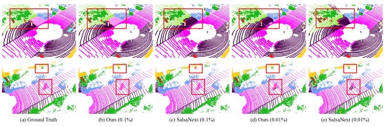
$\blacksquare$bicycle  $\blacksquare$car  $\blacksquare$motorcycle  $\blacksquare$truck  $\blacksquare$other vehicle  $\blacksquare$person  $\blacksquare$bicyclist  $\blacksquare$motorcyclist  $\blacksquare$road  $\blacksquare$parking 
$\blacksquare$sidewalk  $\blacksquare$other ground  $\blacksquare$building  $\blacksquare$fence  $\blacksquare$vegetation  $\blacksquare$trunk  $\blacksquare$terrain  $\blacksquare$pole  $\blacksquare$traffic sign

Figure 2: Sampled predictions on SemKITTI [Behley et al.(2019)Behley, Garbade, Milioto, Quenzel, Behnke, Stachniss, and Gall] validation set.

4.3 Ablation Study

We first vary the backbone used and then ablate our method. Unless otherwise mentioned, we employ SalsaNet backbone with 0.1% annotation evaluated on SemKITTI val. set.

Choice of Backbones. To demonstrate our approach is architecture-agnostic, Tab. 3 shows experiments on the val. sets of SemKITTI [Behley et al.(2019)Behley, Garbade, Milioto, Quenzel, Behnke, Stachniss, and Gall] and SemPOSS [Pan et al.(2020)Pan, Gao, Mei, Geng, Li, and Zhao] with various backbones, namely: RangeNet-21 [Milioto et al.(2019)Milioto, Vizzo, Behley, and Stachniss], SqueezeSegV3-21 [Xu et al.(2020a)Xu, Wu, Wang, Zhan, Vajda, Keutzer, and Tomizuka], and SalsaNext [Cortinhal et al.(2020)Cortinhal, Tzelepis, and Erdal Aksoy] (details in Appendix B.2). For all backbones and datasets, we boost results significantly w.r.t. to the original segmentation backbone, with mIoU difference of $[+3.8,+6.3]$. The results also advocate for our choice of SalsaNext backbone which performs best over all three.

Architectural Components. Tab. 4a shows that all of our designs contribute to the best results. More in depth, ‘w/o contrast module’ shows that the contrastive module (Sec. 3.1) contributes to the biggest gain. To evaluate the benefit of our anchor sampling (Sec. 3.3), ‘w/o anchor sampling’ instead uses all pseudo-labels as anchors showing our strategy is indeed beneficial. In ‘w/o prototype’ we replace our 20 compact prototypes (Sec. 3.2) with 5,000 pixels as in [Wang et al.(2021a)Wang, Zhou, Yu, Dai, Konukoglu, and Gool], showing that our method is lighter and more efficient. Finally, Focal loss (Eq. 3) and Lovasz loss (Eq. 4) are better combined as the two pursue slightly different objectives since Focal loss mitigates imbalance while Lovasz maximizes IoU.

Memory Bank. We now compare other types of memory banks of various per-class sizes. From Tab. 4b, we compare against two variations from [Wang et al.(2021a)Wang, Zhou, Yu, Dai, Konukoglu, and Gool]: ‘Pixel’ stores abundant random pixel-wise embeddings and ‘Region’ which instead stores frame-wise pooled features of semantically consistent regions. Compared to both, our method is more efficient and lighter. The combination of ‘Pixel+Region’ using 10,000 bank size, proves to be better but still gets outperformed with only 20 of our prototypes. Finally, we also compare against prototypes from mini-batch embeddings [Zhuang et al.(2019)Zhuang, Zhai, and Yamins] – which logically perform worse since they fail at capturing the complete dataset knowledge. In a nutshell, Tab. 4 reveals that more stable contrastive targets – like regions or prototypes – are better and that our momentum update mechanism preserves the dataset context thus reaching better performance.

Method	SemPOSS [Pan et al.(2020)Pan, Gao, Mei, Geng, Li, and Zhao]		SemKITTI [Behley et al.(2019)Behley, Garbade, Milioto, Quenzel, Behnke, Stachniss, and Gall]
	mIoU (%)		mIoU (%)
Rangenet-21 [Milioto et al.(2019)Milioto, Vizzo, Behley, and Stachniss]	25.1		40.7
Ours (Rangenet-21)	28.9	+3.8	44.5	+3.8
SqueezeSegV3-21 [Xu et al.(2020a)Xu, Wu, Wang, Zhan, Vajda, Keutzer, and Tomizuka]	30.4		42.5
Ours (SqueezeSegV3-21)	36.7	+6.3	48.5	+6.0
SalsaNext [Cortinhal et al.(2020)Cortinhal, Tzelepis, and Erdal Aksoy]	38.9		52.4
Ours (SalsaNext)	43.0	+4.1	57.6	+5.2

Table 3: COARSE3D with different backbones using 0.01% annotation (val. set).

Method mIoU (%) Ours 57.57 w/o contrast module 55.44 w/o anchors sampling 56.32 w/o prototype (5k pxl) 56.10 w/o voxel propagation 56.26 w/o Focal loss 42.41 w/o Lovász loss 56.10	Memory bank Bank size mIoU (%) $w/o$ contrast - 55.44 Pixel 5,000 56.10 Region 5,000 56.66 Pixel + Region 10,000 56.79 Prototype (mini-batch) 20 56.46 Prototype (ours) 20 57.57	# Prototype mIoU (%) 1 55.47 10 56.15 20 57.57 50 56.18 100 56.89
(a) Method ablation	(b) Memory bank	(c) Prototypes number

Strategy Basis mIoU(%) All No 56.32 Random K 56.06 Hard-threshold Softmax 57.09 Top-K 56.11 Probability 56.93 Hard-threshold Entropy 56.38 Top-K 56.30 Probability (Ours) 57.57	Strategy mIoU(%) Easy 56.15 Hard $\underline{57.00}$ Semi Hard 56.59 Random 56.41 All (Ours) 57.57	Anno. mIoU (%) SalsaNext [Cortinhal et al.(2020)Cortinhal, Tzelepis, and Erdal Aksoy] Ours 0.001% 30.39 31.69 0.01% 44.00 47.13 0.1% 52.43 56.61 1% 56.16 58.30 100% 56.44 58.39
(d) Anchor sampling	(e) Key sampling	(f) Annotation

Table 4: Ablation study results on SemKITTI[Behley et al.(2019)Behley, Garbade, Milioto, Quenzel, Behnke, Stachniss, and Gall] validation set.

Number of Prototypes. Tab. 4c studies the impact of varying the number of per class prototypes from 1 to 100. With only 1 prototype, each class uses a single high-dimensional embedding which is also referred to as class-wise memory bank [Alonso et al.(2021)Alonso, Sabater, Ferstl, Montesano, and Murillo]. Altogether, 20 prototypes are optimal among tested choices since fewer or more prototypes degrade performance.

Choice of Anchors. We study the choice of anchors in Tab. 4d, by varying the basic function used for sampling (col ‘Basis’) and the strategy for sampling segmentation features (col ‘Strategy’). Without any basis function, we tried using all pseudo labels predictions ‘All’ or a ‘Random X’ number of X pixels. Results show that more support from pseudo labels boosts performance but the strategy is suboptimal given the prediction inaccuracies. To mitigate this, we evaluate the predictions quality with a basis function: either a ‘Softmax’ as [Rizve et al.(2021)Rizve, Duarte, Rawat, and Shah] or our ‘Entropy’ proposal (Sec. 3.3). For both ‘Softmax’ and ‘Entropy’ basis, we consider sampling with a finetuned ‘hard-threshold’, the ‘Top-X’ elements, or selection from a random ‘Probability’ sampling. Our ‘Entropy’ driven probability sampling performs best. We relate these results to the fact that Shannon entropy stores joint information distribution for all class predictions, which makes it more insightful for a proper anchor selection.

Choice of Keys. Prior research [Wang et al.(2021a)Wang, Zhou, Yu, Dai, Konukoglu, and Gool, Robinson et al.(2020)Robinson, Chuang, Sra, and Jegelka] show the benefit of using smart key sampling strategies which differs to our use of all keys. In Tab. 4e we compare the common key sampling strategies being ‘easy’, ‘hard’, ‘semi-hard’, ‘random’ or ‘All’. Except for the ‘All’ strategy, we consider 100 prototypes and use the key sampling mentioned to select 20 of these prototypes as keys. In short, ‘easy’/‘hard’ indicates the complexity for anchors to learn with such keys. We refer to [Wang et al.(2021a)Wang, Zhou, Yu, Dai, Konukoglu, and Gool] for details. Intuitively, using semi-hard or hard keys encourage the network to learn more robust representations. However, we denote that using all keys performs in fact better with our prototypes. We conjecture that this relates to the prototype capturing a more robust dataset context which is beneficial to preserve.

Effect of Annotation. In Tab. 4f we vary the annotation ratio from 100% (full supervision) to only 0.001% (roughly 1 point label per frame), showing our robustness to the most extreme cases – despite a drastic mIoU drop for 0.001% annotation due to rare classes being absent from labels. In fact, reporting for the latter only mIoU for ‘classes in labels’, SalsaNext and Ours get respectively, 45.50% and 47.61% which again demonstrates robustness. We further study the effect of random label in Appendix A, showing in a nutshell that variances of 0.1%/0.01% settings are $\pm$0.93/$\pm$0.32 – far smaller than the baseline gaps (+4.18/+3.13).

5 Conclusion

In this paper, we present a weakly supervised LiDAR point cloud semantic segmentation framework. Specifically, we develop a compact class-prototype contrastive learning scheme based on online clustered embeddings and use this prototype as the key to pulling entropy-driven sampled anchors. Extensive experiments on three projection-based backbones and three real-world datasets demonstrate the effectiveness of our method.

Acknowledgement. Rong Li was supported by the SMIL lab of South China University of Technolog, received support and advices from Prof. Mingkui Tan, Prof. Caixia Li and Zhuangwei Zhuang. Rong Li was also partly supported by Key-Area Research and Development Program Guangdong Province (2019B010155001). Inria members were partly funded by French project SIGHT (ANR-20-CE23-0016). This work was performed using HPC resources from GENCI–IDRIS (Grant 2021-AD011012808 and 2022-AD011012808R1).

We study the effect of annotation sampling in Appendix A and report implementation details with new ablation in Appendix B and more qualitative results in Appendix C.

Appendix A Effect of Annotations

In weak supervision settings, changing the set of labelled points impact performance. We now study more in depth the effect of sampled labels by randomly resampling labels 3 times on 2 datasets. As it appears in Tab. 5, our method is relatively stable (i.e., $\text{std}{<}1$). We also measure the gap between random annotations and those of human by asking 2 operators to annotate the entire SemPOSS, labeling roughly 0.01% points per frame. Again, from Tab. 5 our ‘human’ labels are within 3 std of the mean 0.01% performance (i.e., 29.27 vs 31.48$\pm 0.43$).

	SemKITTI [Behley et al.(2019)Behley, Garbade, Milioto, Quenzel, Behnke, Stachniss, and Gall]		SemPOSS [Pan et al.(2020)Pan, Gao, Mei, Geng, Li, and Zhao]
Anno.	0.10%	0.01%	0.10%	0.01%	human ($\approx{}$0.01%)
run 1	57.57	47.35	43.00	31.10	29.27
run 2	56.54	47.28	42.88	31.95	-
run 3	55.71	46.76	42.47	31.38	-
all	56.61$\pm$0.93	47.13$\pm$0.32	42.78$\pm$0.28	31.48$\pm$0.43	-

Table 5: Effect of annotation sampling on SemKITTI and SemPOSS.

Appendix B Implementation Details

B.1 Label Voxel Propagation

We replicate SQN [Hu et al.(2022)Hu, Yang, Fang, Guo, Leonardis, Trigoni, and Markham] and apply their random grid downsampling with 0.06 voxel size. Our trivial scheme simply propagates existing labels to all points within the same voxel – thus densifying the labels at no extra labelling cost. In the extremely rare case of conflicting labels within a single voxel (e.g. a voxel having two labelled points with different classes), the voxel label will be randomly assigned.

We evaluate the effect of this voxel propagation scheme using the SalsaNext backbone on SemKITTI val. set in the 0.1% annotation setting. With/without our scheme we get 57.57/56.26 mIoU. Since baselines do not use our label propagation, it is important to note that the mIoU gap obtained (+1.31 mIoU) is smaller than the gap with the original SalsaNext (+5.14, cf. main paper Tab. 3f) in the same 0.1% setting. This advocates that our method only partly benefits from our voxel propagation scheme and performs best thanks to our overall contrastive learning strategy.

B.2 Segmentation Backbones

SalsaNext [Cortinhal et al.(2020)Cortinhal, Tzelepis, and Erdal Aksoy]. We use the official implementation for the SemKITTI dataset[Behley et al.(2019)Behley, Garbade, Milioto, Quenzel, Behnke, Stachniss, and Gall] and applied our best effort to fairly re-implement it for nuScenes [Caesar et al.(2020)Caesar, Bankiti, Lang, Vora, Liong, Xu, Krishnan, Pan, Baldan, and Beijbom] and SemPOSS [Pan et al.(2020)Pan, Gao, Mei, Geng, Li, and Zhao]. Specific to SemPOSS[Pan et al.(2020)Pan, Gao, Mei, Geng, Li, and Zhao], we used an input padding to get a compatible size. When trained with our method, we finetune our contrastive learning hyperparameters.

SqueezeSegV3 [Xu et al.(2020a)Xu, Wu, Wang, Zhan, Vajda, Keutzer, and Tomizuka]. We use the lighter SqueezeSegV3-21 from the official implementation. To boost performance on weakly supervised tasks, we replaced the multi-layer cross-entropy loss – improper for sparse weak labels due to its downsampling –, with normal cross-entropy loss. When trained with our method, we simply use the contrastive learning hyperparameter found with SalsaNext.

RangeNet++ [Milioto et al.(2019)Milioto, Vizzo, Behley, and Stachniss]. We use the ligher RangeNet-21 from the official implementation. Inputs are pad to get compatible size. When trained with our method, we simply use the contrastive learning hyperparameter found with SalsaNext.

Appendix C Additional Results

We report additional qualitative results using SalsaNext on SemKITTI, SemPOSS, and nuScenes in Figs. 3, 4 and 5, respectively, for both 0.1% and 0.01% settings. Overall, our method surpasses SalsaNext, especially in ambiguous and cluttered regions, illustrated in Fig. 3 (sidewalk/parking - row 1; vegetation/building - row 3), in Fig. 4 (car - row 1; rider - row 3; pole/plants - row 4), and in Fig. 5 (terrain/other flat - row 1). Also, SalsaNext makes more mistake regarding classes with close semantical meaning as in Fig. 3 (truck/car - row 1), in Fig. 4 (building/fence - row 5), and in Fig. 5 (bus/trailer/truck - row 2, 3, 4, 5). Furthermore, our method shows superiority in predicting small objects with similar structure or spatial position, demonstrated in Fig. 3 (fence/vegetation - row 4, 5; trunk/traffic sign - row 5), in Fig. 4 (rider/people - row 2, 3, 5; pole/plants - row 4), and in Fig. 5 (terrain/other flat - row 1). Additionally, our method infers better far away, low density regions e.g. Fig. 4 (car - row 1), and Fig. 5 (vegetation/barrier - row 2).

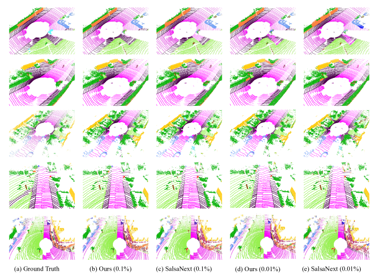
$\blacksquare$bicycle  $\blacksquare$car  $\blacksquare$motorcycle  $\blacksquare$truck  $\blacksquare$other vehicle  $\blacksquare$person  $\blacksquare$bicyclist  $\blacksquare$motorcyclist  $\blacksquare$road  $\blacksquare$parking 
$\blacksquare$sidewalk  $\blacksquare$other ground  $\blacksquare$building  $\blacksquare$fence  $\blacksquare$vegetation  $\blacksquare$trunk  $\blacksquare$terrain  $\blacksquare$pole  $\blacksquare$traffic sign

Figure 3: Additional qualitative results on SemKITTI [Behley et al.(2019)Behley, Garbade, Milioto, Quenzel, Behnke, Stachniss, and Gall]

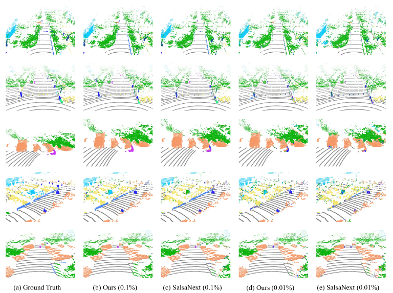
$\blacksquare$people  $\blacksquare$rider  $\blacksquare$car  $\blacksquare$trunk  $\blacksquare$plants  $\blacksquare$traffic-sign 
$\blacksquare$pole  $\blacksquare$trashcan  $\blacksquare$building  $\blacksquare$cone/stone  $\blacksquare$fence  $\blacksquare$bike  $\blacksquare$road

Figure 4: Qualitative results on SemPOSS [Pan et al.(2020)Pan, Gao, Mei, Geng, Li, and Zhao]

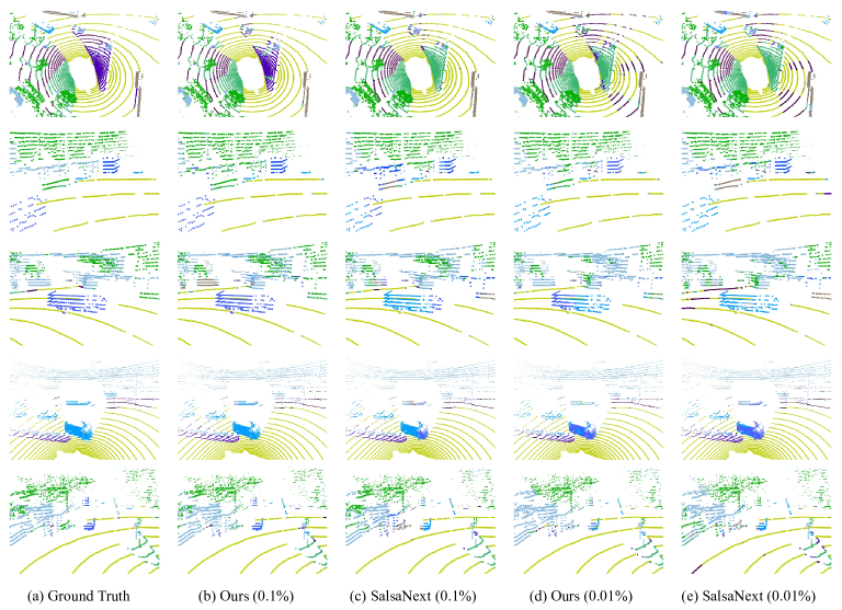
$\blacksquare$barrier  $\blacksquare$bicycle  $\blacksquare$bus  $\blacksquare$car  $\blacksquare$construction vehicle  $\blacksquare$motorcycle  $\blacksquare$pedestrian  $\blacksquare$traffic cone  $\blacksquare$trailer 
$\blacksquare$truck  $\blacksquare$driveable surface  $\blacksquare$other flat  $\blacksquare$sidewalk  $\blacksquare$terrain  $\blacksquare$manmade  $\blacksquare$vegetation

Figure 5: Qualitative results on nuScenes [Caesar et al.(2020)Caesar, Bankiti, Lang, Vora, Liong, Xu, Krishnan, Pan, Baldan, and Beijbom]

References

- [Aksoy et al.(2020)Aksoy, Baci, and Cavdar] Eren Erdal Aksoy, Saimir Baci, and Selcuk Cavdar. Salsanet: Fast road and vehicle segmentation in lidar point clouds for autonomous driving. In IV, 2020.
- [Alonso et al.(2021)Alonso, Sabater, Ferstl, Montesano, and Murillo] Inigo Alonso, Alberto Sabater, David Ferstl, Luis Montesano, and Ana C Murillo. Semi-supervised semantic segmentation with pixel-level contrastive learning from a class-wise memory bank. In ICCV, 2021.
- [Behley et al.(2019)Behley, Garbade, Milioto, Quenzel, Behnke, Stachniss, and Gall] Jens Behley, Martin Garbade, Andres Milioto, Jan Quenzel, Sven Behnke, C. Stachniss, and Juergen Gall. Semantickitti: A dataset for semantic scene understanding of lidar sequences. In ICCV, 2019.
- [Bell and Bala(2015)] Sean Bell and Kavita Bala. Learning visual similarity for product design with convolutional neural networks. In TOG, 2015.
- [Berman et al.(2018)Berman, Triki, and Blaschko] Maxim Berman, Amal Rannen Triki, and Matthew B Blaschko. The lovász-softmax loss: A tractable surrogate for the optimization of the intersection-over-union measure in neural networks. In CVPR, 2018.
- [Bucher et al.(2016a)Bucher, Herbin, and Jurie] Maxime Bucher, Stéphane Herbin, and Frédéric Jurie. Hard negative mining for metric learning based zero-shot classification. In ECCV, 2016a.
- [Bucher et al.(2016b)Bucher, Herbin, and Jurie] Maxime Bucher, Stéphane Herbin, and Frédéric Jurie. Improving semantic embedding consistency by metric learning for zero-shot classiffication. In ECCV, 2016b.
- [Caesar et al.(2020)Caesar, Bankiti, Lang, Vora, Liong, Xu, Krishnan, Pan, Baldan, and Beijbom] Holger Caesar, Varun Bankiti, Alex H. Lang, Sourabh Vora, Venice Erin Liong, Qiang Xu, Anush Krishnan, Yu Pan, Giancarlo Baldan, and Oscar Beijbom. nuscenes: A multimodal dataset for autonomous driving. In CVPR, 2020.
- [Cai et al.(2020)Cai, Frankle, Schwab, and Morcos] Tiffany Tianhui Cai, Jonathan Frankle, David J Schwab, and Ari S Morcos. Are all negatives created equal in contrastive instance discrimination? In arXiv, 2020.
- [Chaitanya et al.(2020)Chaitanya, Erdil, Karani, and Konukoglu] Krishna Chaitanya, Ertunc Erdil, Neerav Karani, and Ender Konukoglu. Contrastive learning of global and local features for medical image segmentation with limited annotations. In NeuRIPS, 2020.
- [Chen et al.(2020a)Chen, Kornblith, Norouzi, and Hinton] Ting Chen, Simon Kornblith, Mohammad Norouzi, and Geoffrey E. Hinton. A simple framework for contrastive learning of visual representations. In ICML, 2020a.
- [Chen et al.(2020b)Chen, Fan, Girshick, and He] Xinlei Chen, Haoqi Fan, Ross Girshick, and Kaiming He. Improved baselines with momentum contrastive learning. In arXiv, 2020b.
- [Chen et al.(2022)Chen, Nießner, and Dai] Yujin Chen, Matthias Nießner, and Angela Dai. 4dcontrast: Contrastive learning with dynamic correspondences for 3d scene understanding. In ECCV, 2022.