Supervised Parameter Estimation of Neuron Populations from Multiple Firing Events

Abstract

The firing dynamics of biological neurons in mathematical models is often determined by the model’s parameters, representing the neurons’ underlying properties. The parameter estimation problem seeks to recover those parameters of a single neuron or a neuron population from their responses to external stimuli and interactions between themselves. Most common methods for tackling this problem in the literature use some mechanistic models in conjunction with either a simulation-based or solution-based optimization scheme. In this paper, we study an automatic approach of learning the parameters of neuron populations from a training set consisting of pairs of spiking series and parameter labels via supervised learning. Unlike previous work, this automatic learning does not require additional simulations at inference time nor expert knowledge in deriving an analytical solution or in constructing some approximate models. We simulate many neuronal populations with different parameter settings using a stochastic neuron model. Using that data, we train a variety of supervised machine learning models, including convolutional and deep neural networks, random forest, and support vector regression. We then compare their performance against classical approaches including a genetic search, Bayesian sequential estimation, and a random walk approximate model. The supervised models almost always outperform the classical methods in parameter estimation and spike reconstruction errors, and computation expense. Convolutional neural network, in particular, is the best among all models across all metrics. The supervised models can also generalize to out-of-distribution data to a certain extent.

1 Introduction

It is well known that neurons in our brain can produce very complicated spiking patterns, including a few different types of neural oscillations. Some oscillations can be reproduced by mathematical neuron models at a certain level. In particular, a spiking pattern named multiple firing event (MFE) is observed in many neuronal network models Chariker; rangan2013dynamics; rangan2013emergent; zhang2014coarse. In an MFE, a certain proportion of neurons in the population, but not all of them, fires a spike during a relatively short time window and forms a spike volley. Similar spiking patterns that lie between homogeneity and synchrony have been observed in many experimental studies. It is believed that MFEs are responsible for the Gamma rhythm in the central nervous system rangan2013dynamics; rangan2013emergent; henrie2005. In general, MFE can be observed in neuronal populations with both excitatory and inhibitory neurons when the parameters are suitable. An MFE is caused by a balance of recurrent excitation and inhibition from neurons. Spikes of excitatory neurons excite both excitatory and inhibitory populations. The former induces a cascade of spiking activities, while the latter forms an inhibitory current that stops the spiking volley. Neuronal networks with MFEs are intrinsically multi-scale because of the rapid spiking activities during MFEs.

Despite the intuitive mechanism of MFEs and some early investigation about the low dimension nature of MFEs cai2022model, it is very difficult to find a low dimensional dynamical system to accurately approximate the MFEs. Known results about MFE mechanism in zhang2014coarse; li2019stochastic; cai2022model do not provide a full answer to that. Spiking activities in MFEs can range from quite homogeneous to very synchronous. However, no existing theory can accurately predict the spiking pattern without running the full model, nor infer parameters from the spiking activities. In this paper, we attempt to shed some light on this challenging problem by training supervised machine learning models to learn the spiking activities of MFEs. More precisely, we generate many spike series from a wide range of parameters using a stochastic neuronal network model introduced in Li2017HowWD. These series are then labeled by the corresponding parameters as a training set. After some training, supervised models including a convolutional neural network, deep neural network, random forest, and support vector regression can backwardly infer the parameters from which the spike series were obtained.

The result is very encouraging. Although the neuronal population model has a lot of stochasticity and the MFEs have high volatility, our supervised models, especially the convolutional neural network (CNN), successfully grasp the key relation between parameters and spiking patterns. When an input spiking pattern is given to the CNN, the predicted parameters can produce a visually similar spiking pattern. These similarities can be quantified by various reconstruction error measures. The resulting reconstruction errors from supervised models are low and can be largely attributed to the inherent stochasticity of the neuronal network model that generated the data. Further, the supervised models are benchmarked against traditional approaches in parameter estimation including a genetic search, Sequential Neural Posterior Estimation (SNPE), and a random walk approximate model.

Further numerical experiments also confirm that supervised models, especially neural networks, have some generalization ability. When the spike series is generated by a parameter set that is deliberately sampled outside of the training set, the supervised models can still reconstruct the spike series reasonably well. In both the test and generalization experiments, the convolutional neural network has the best performance while incurring a relatively low computation cost.

The organization of this paper is as follows. Section 2 reviews some classical approaches in the literature and their drawbacks. Section 3 describes the supervised learning approach, the data-generating neuronal network model, data generation process, a regularization heuristic to aid learning, and some classical models that we benchmarked against. In Section LABEL:sec:res, we report the results on the test and generalization datasets. Section LABEL:sec:con is the conclusion. Appendices LABEL:sec:pars and LABEL:sec:model_configs detail the parameter settings and model configurations used.

2 Related Work

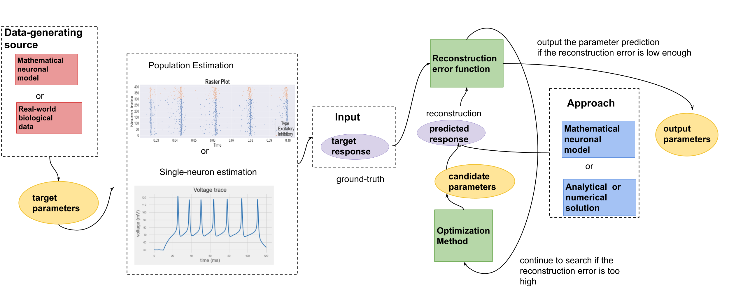
Figure 1: An overview of traditional approaches to parameter estimation. A target response is given. An optimization routine is used to produce a candidate parameter set. The parameter set is then used to produce a predicted response either by a simulator or some approximation solution. The predicted response is compared against the target one using some reconstruction error function. This procedure ceases when the predicted response is deemed similar enough to the target.

Parameter estimation is a difficult and well-studied problem in the literature. Most traditional approaches proceed as follows (see Figure 1). A target spike count input, in the case of population estimation, or a voltage trace, in the case of single-neuron estimation, is given, either from synthetic data generated by a mathematical model or from biological experiments (e.g., MCMC; evol). The input is typically vectorized, for example by discretizing into time series or extracting summary features such as the average spike height and firing rate review. Then, an optimization framework is used to search through the parameter space and select a candidate parameter set that is likely to produce a neural response similar to the target response. The reconstructed response can be obtained in two main ways. Some methods use a neuronal model as a simulator. Others obtain the signal through solving some differential equations, describing the dynamics of the neurons. For example, pde solves a Fokker-Planck PDE numerically while single obtains the solution to the Hodgkin-Huxley neuronal model hodgkin analytically. Sometimes, an approximate model where an analytical solution is available, for example a Poisson process in pde, or some other surrogate models zhang2020DNN are used. The reconstructed response is then compared to the ground truth using some loss function. If the loss is low enough, then the current parameter set is outputted, and this procedure stops. Otherwise, we continue to search through the parameter space.

There are many search methods available such as likelihood-free Bayesian inference bayesian; snpe, evolutionary algorithm evol, Simplex simplex, interior point line search offset, particle swarm optimization and MCMC MCMC, and interval analysis based optimization single. The paper review reviews some other search algorithms such as simulated annealing and gradient descent.

In those works, there is additional time required in running extra simulations (simulator-based) or in numerically solving some differential equations (solution-based) to construct predicted responses at inference time. The computation cost in iteratively searching through the parameter space can also be high. In the case of solution-based approaches, expert knowledge is also required in constructing the differential equations, and their analytical solutions or approximation. Table 1 compares our approaches to some others. Note that the supervised learning approach in this paper does not require additional simulations other than the ones used to generate the training data or any expert knowledge. Most works that we encountered (including evol; MCMC; snpe) estimate the parameters of a single neuron. In our work, we found that parameter estimation at a population level using these methods requires simulating a large number of neuron populations at inference time and therefore sharply increases the computation expense.

Table 1: Comparing some approaches to parameter estimation.

Approach	Require simulations at inference?	Solution-based
evol	yes	no
bayesian	yes	no
simplex	yes	no
pde	no	yes
offset	yes	no
MCMC	no	yes
single	no	yes
lfp	yes	no
Supervised learning (ours)	no	no

The supervised learning approach here is most similar to the work of lfp, which uses a convolution neural network to learn neuronal parameters from local field potentials (LFPs). The key difference between our work and theirs is that while they extract high-level features, namely 6-channels LFPs, from spiking trains as input, we use the raw spike series. Obtaining local field potentials requires replaying the generated spike trains from a neuron model to a more biophysically detailed model, thus adding more computation cost. Deep learning models have been observed to be able to automatically extract high-level and useful features from data (for example, in image processing cnn_review, natural language processing text or neuron response features snpe). Thus, we chose to feed in the raw spike series as inputs.

The paper zhang2020DNN uses a deep neural network (DNN) to learn a surrogate forward model mapping neuronal parameters to high-level features of the spike trains, i.e., their firing rates. Then, another outer search is required to do parameter tuning similar to Figure 1. In contrast to this approach, we use high-dimensional spike series as inputs, which allow us to learn the inverse mapping from neuronal responses to parameters directly.

Another work snpe also uses neural networks. There, neural networks were used as density estimators in a sequential Bayesian framework, also requiring a lot of simulations at inference time.

The supervised learning approach explained in the next section will make a distinction between training and inference stages. Most computation time is invested in the training stage so that inferences on a new data point can be done almost instantaneously.

3 Methods

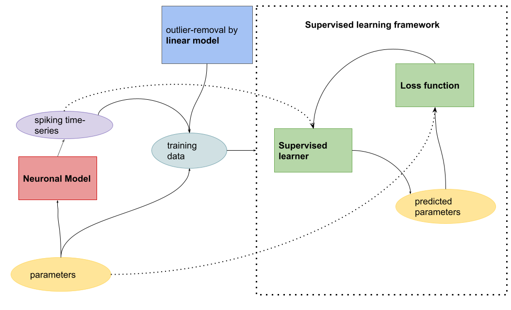
Figure 2: Supervised learning framework to parameter estimation. The training data consisting of the spiking time series and parameter labels is fed to a supervised learning model. To ensure the quality of the training data, we also use an outlier removal procedure (see Section 3.4).

3.1 Supervised Learning Approach

The approach we chose is to frame the parameter estimation as a supervised learning problem (see Figure 2). Note that, unlike previous search approaches that we have discussed, supervised learning requires the parameter labels as inputs along with the usual spiking time series. We will discuss more the process of constructing spiking time series in Section 3.3. Requiring parameter labels is usually not a severe constraint since there is often some mechanistic model available to generate synthetic data. For those mechanistic models, we can control the parameters, and thus know their values.

This supervised learning approach proceeds by generating a large number of parameter set and spike series pairs. At training time, supervised models have to learn to perform accurate parameter prediction. In general, a supervised learner tries to minimize the average prediction loss on the training set (i.e., the empirical risk)

$$\mathcal{L}=\frac{1}{N}\sum_{i=1}^{N}L(\underline{y}_{i},\underline{\hat{y}_{i}})$$ (1)

where $N$ is the training set size, $\underline{y}_{i}$ is the true parameter set, $\underline{\hat{y}_{i}}$ is the estimated parameter set, and $L$ is some loss function. In this paper, we choose $L$ to be the mean absolute error (MAE) i.e., $L(\underline{y},\underline{\hat{y}})=\ell_{1}(\underline{y}-\underline{\hat{y}})$ where $\ell_{1}$ is the L1 norm. MAE was chosen since we have found that it is less sensitive to outliers than other loss functions such as the mean squared error.

At inference, a target spike series is given without a label, and the models will then try to recover the parameters without needing additional simulations. We also include an outlier removal procedure Section 3.4 to ensure the quality of the training data.

3.2 Neuronal Model

In this section, we will describe the neuronal model used to generate data. Mathematical neuronal models in the literature come in great variety, varying in complexity. For example, the complex Hodgkin-Huxley equations hodgkin model each ion channel within a neuron explicitly while much simpler mean-field methods such as the Wilson-Cowan equation meanfield models some averaged quantities of neurons such as firing rate over time. In choosing which neuronal model to use, there is a trade-off between biological realism and tractability: more realistic models tend to contain quantities that are harder to measure experimentally or computationally expensive to simulate. A popular class of models at an intermediate level of complexity is integrate-and-fire iaf1; iaf2, which can generate a diverse set of firing dynamics. The model that we use for this study, from Li2017HowWD, is of the integrate-and-fire class with some known theoretical properties.

3.2.1 Description of the Model

The model used in this paper is a stochastic integrate-and-fire type. Instead of modeling physiological details such as ion channels, we only keep track of the electrical property of a neuron – its membrane potential. The membrane potential of a neuron changes after receiving external or in-network stimuli. A spike is fired when the membrane potential reaches a certain threshold potential.

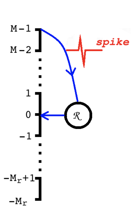
Figure 3: Each neuron’s membrane potential is discretized into the range $[-M_{r},M]\cup\mathcal{R}$. The voltage is set to $\mathcal{R}$ after a spike. When the neuron comes out of refractory, the voltage starts at $0$.

The model consists of a local population of $N_{E}$ excitatory (E) and $N_{I}$ inhibitory (I) neurons. Each neuron has a membrane potential, which we assume to take on finitely many values in $\{-M_{r},-M_{r}+1,...,0,...,M\}\cup\{\mathcal{R}\}$, where $M_{r},M\in\mathbb{N}$ and $\mathcal{R}$ is a special state, called refractory. A neuron in this refractory state is “asleep” and cannot be affected by stimulus. The minimum possible potential $-M_{r}$ is known as the reversal potential. When the voltage $V_{i}$ of the $i^{th}$ neuron reaches the voltage threshold $M$, the neuron is said to spike or fire and $V_{i}$ is set to $\mathcal{R}$. In other words, the neuron enters a refractory period after spiking (see Figure 3).

There are two mechanisms for changing the voltage $V_{i}$: background stimuli and neuron-to-neuron interactions. In the background, there is an external drive that increases the membrane potentials. This external drive can be thought of as inputs from a neighboring neuronal population or from sensory input. Mathematically, we represent the external inputs as Poisson processes delivering impulsive kicks to each neuron independently. These inputs always increase the membrane potentials by $1$. We have two Poisson arrival processes parametrized by $\lambda^{E},\lambda^{I}>0$, representing the rates of the Poisson kicks to $E$ and $I$ neurons respectively. Under these Poisson processes, the time between two consecutive kicks is exponentially distributed, and the number of kicks over a given time interval is Poisson distributed.

Within the population, there are opportunities for changing membrane potentials whenever a neuron spikes. When a neuron fires, the neuron sends a signal (via neurotransmitters) to its post-synaptic neurons. The set of post-synaptic neurons is randomly and dynamically chosen as needed. Specifically with $Q^{\prime},Q\in\{E,I\}$, when a Q’-type neuron fires, each Q-type neuron has the probability of $P_{QQ^{\prime}}$, independent of other neurons, of being connected to the spiking neuron. $P_{QQ^{\prime}}\in[0,1]$ is called the connectivity probability. As such, the set of post-synaptic neurons to a given neuron is not fixed and is chosen anew every time. This follows the convention from the paper Li2017HowWD.

Each signal from $Q^{\prime}$-type neuron to $Q$-type neuron carries a weight of $S_{QQ^{\prime}}$, where $S_{QQ^{\prime}}\in\mathbb{Z^{+}}$ if $Q^{\prime}=E$ and $S_{QQ^{\prime}}\in\mathbb{Z^{-}}$ if $Q^{\prime}=I$. That is to say, an excitatory signal increases the post-synaptic neuron’s voltage while an inhibitory signal decreases the voltage. Upon arrival to the post-synaptic neuron $i$, the signal alters $V_{i}$ precisely by $S_{QQ^{\prime}}$ i.e.,  $V_{i}=V_{i}+S_{QQ^{\prime}}$. There is a random delay in neuron-to-neuron signal delivery. Each signal arrives at its destination after an exponentially distributed delay time with mean $\tau^{Q^{\prime}}$. Note that the delay time of each signal is only dependent on the type of presynaptic neuron (excitatory or inhibitory) and is independent between signals.

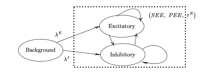
Figure 4: There are two types of stimuli: background and neuron-to-neuron. The background inputs are parametrized by $\lambda^{E},\lambda^{I}$, depending on the type of receiving neurons. The in-population interaction from $Q^{\prime}$-type to $Q$-type neuron is parametrized by $(S_{QQ^{\prime}},P_{QQ^{\prime}},\tau^{Q^{\prime}})$ – the kick strength, connectivity probability and mean delay time.

We now describe a neuron’s refractory period. After a neuron spikes, it enters a recovery period known as refractory. During this period, any background kick or signal from other neurons will not alter the neuron’s potential. The neuron stays in refractory for an exponentially distributed amount of time with mean $\tau_{\mathcal{R}}$. After this period, the voltage is set to $0$ and the neuron behaves as usual with respect to stimuli.

The illustration of the neuronal model’s description is in Figure 4. Table 2 summarizes all of the parameters in this neuronal model.

Table 2: A list of parameters in the data-generating neuronal model.

Parameters	Description
$M$	Maximal neuronal voltage (firing threshold)
$-M_{r}$	Minimum neuronal voltage
$N_{E}$	Number of excitatory neurons in the population.
$N_{I}$	Number of inhibitory neurons in the population.
$\lambda_{E}$	Rate of external stimulus to E-population.
$\lambda_{I}$	Rate of external stimulus to I-population.
$P_{EE}$	Probability of E-to-E dynamic synaptic connection.
$P_{IE}$	Probability of E-to-I dynamic synaptic connection.
$P_{EI}$	Probability of I-to-E dynamic synaptic connection.
$P_{II}$	Probability of I-to-I dynamic synaptic connection.
$S_{EE}$	Synaptic strength for E-to-E connection.
$S_{IE}$	Synaptic strength for E-to-I connection.
$S_{EI}$	Synaptic strength for I-to-E connection.
$S_{II}$	Synaptic strength for I-to-I connection.
$\tau_{R}$	Mean refractory time
$\tau_{E}$	Mean E-kick delay time from an excitatory presynaptic neuron
$\tau_{I}$	Mean I-kick delay time from an inhibitory presynaptic neuron

3.2.2 Known Theoretical Properties

It is proven in the paper Li2017HowWD that the neuronal model is a countable state Markov process that admits a unique invariant probability distribution. In addition, the speed of convergence towards this invariant probability distribution is exponentially fast. In li2019stochastic; li2020entropy, it is further shown that many statistical properties of MFEs, including spiking count, variance, and entropy, are both well-defined and computable under this model.

3.2.3 Firing Dynamics

The neuronal model can cover a wide range of spiking patterns from almost homogeneous to fully synchronous. In this section, we demonstrate a gallery of neuronal responses produced by the model by varying its parameters. We generate three neuron populations by fixing the parameter values as given in Table LABEL:tab:static_params and means of the ranges for other parameters in Table LABEL:tab:dynamic_params while varying one parameter $\tau_{E}$ (mean excitatory kick delay time) as follows.

1. The “Homogeneous” population, abbreviated as “Hom” in the Figure.

   $$\tau_{E}=9\textrm{ ms}.$$

2. The “Regular” population, abbreviated as “Reg” in the Figure.

   $$\tau_{E}=5\textrm{ ms}.$$

3. The “Synchronized” population, abbreviated as “Sync” in the Figure.

   $$\tau_{E}=1\textrm{ ms}.$$

The neuronal response is given in Figure 5. As can be observed, the population with a lower $\tau_{E}$ displays a higher degree of synchrony. The synchronization is marked by a high number of spikes in a short duration followed by a period of low spiking activities. In the raster plots, higher synchrony is revealed by the presence of concentrated columns, indicating periods when a lot of neurons fire at once. We also include plots of the fraction of neurons in a population that are firing at a given time. In those plots, synchrony is shown by sharp peaks in the spiking fraction. In the Reg population that lies between the two extremes, one can observe some local peaks in the spiking fraction plot that look distinctive from the more uniform pattern of the Hom population’s plot but not as sharp as those of the Sync population. For the Reg population, one can also see that concentrated columns are beginning to form in the raster plot.

In Figure 6, we demonstrate the effect of varying $S_{EE}$ (E-E kick strength) on the population. We fix the population’s configuration as in the Regular population of Figure 5. $S_{EE}$ is varied as follows.

1. The “Low SEE Homogeneous” population, abbreviated as “Low SEE Hom” in the Figure.

   $$S_{EE}=2.5.$$

2. The “High SEE Synchronized” population, abbreviated as “High SEE Syn” in the Figure.

   $$S_{EE}=10.$$

With $S_{EE}=2.5$, it takes an excitatory neuron in the “Low SEE Homogeneous” population $40$ consecutive excitatory kicks to spike. With $S_{EE}=10$, an excitatory neuron in the “High SEE Synchronized” population only requires $10$ consecutive excitatory kicks to spike. Thus, we observe that the population of the higher $S_{EE}$ value has a higher degree of synchrony and spiking rate.

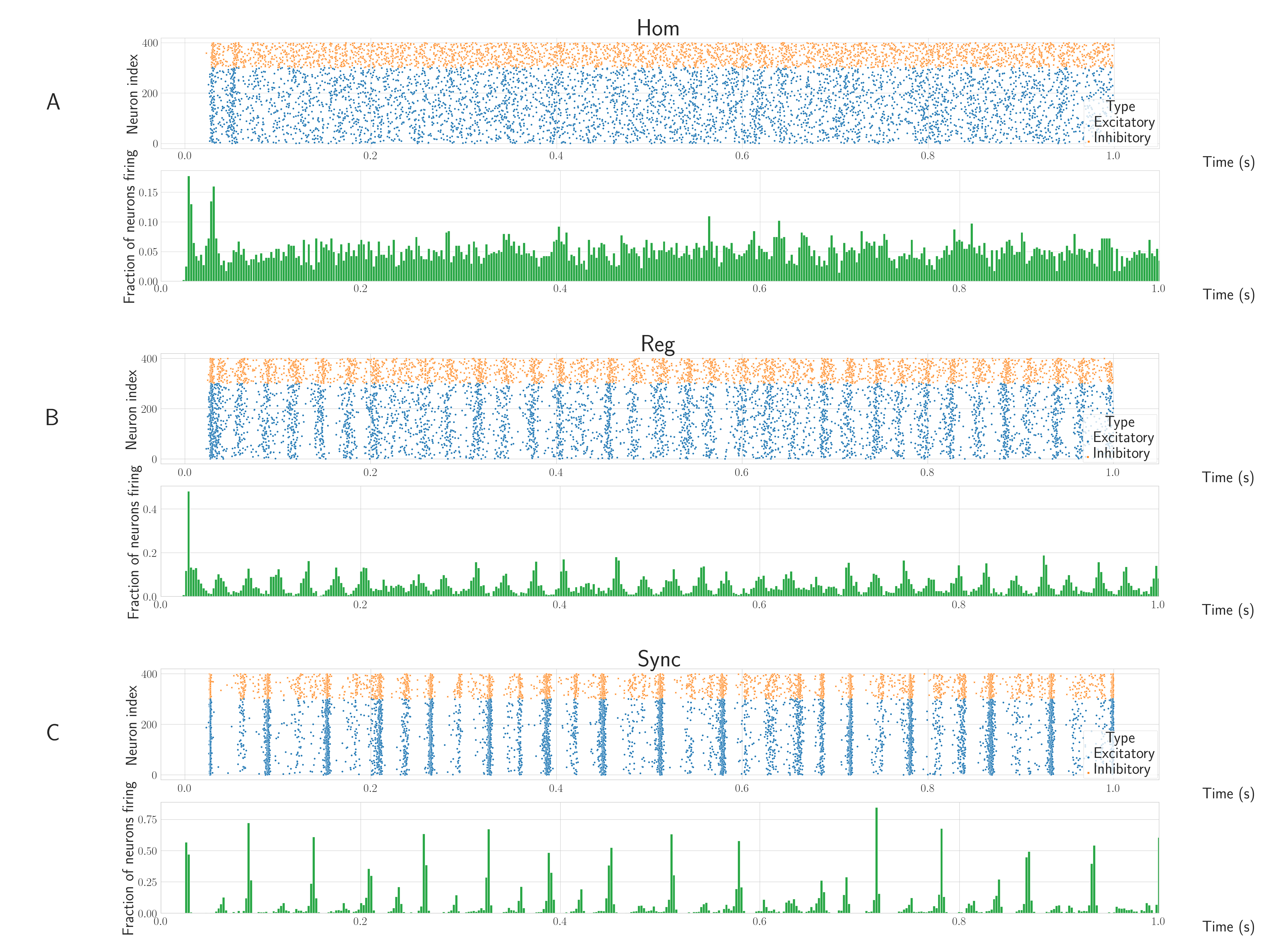
Figure 5: Effect of $\tau_{E}$ on neuron response. Neuronal responses of three neuronal populations, homogeneous (Hom), regular (Reg), and synchronized (Sync), are included. The raster plots display each firing event. Plots of the proportion of neurons in the populations firing at any given time are also included. The homogeneous population tends to have dispersive firing patterns while neurons in the synchronized population tend to fire together. The regular population displays an intermediate firing pattern between homogeneity and synchrony.

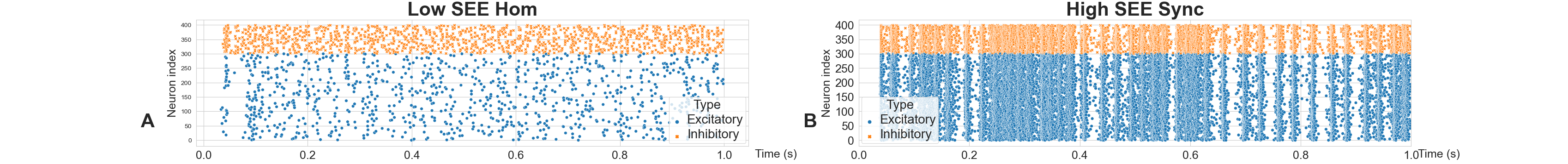
Figure 6: Effect of $S_{EE}$: two neuronal populations of low and high $S_{EE}$ values. The population with the higher $S_{EE}$ value is more synchronized and fires far more frequently.

3.3 Data Generation

In this study, we consider a parameter estimation task on 6 parameters while fixing the other 11 parameters. The 11 static parameters include those specifying the size of the neuronal population, the membrane potential’s range, the external drive strengths, the connectivity probabilities, and the mean refractory time. These parameters are given in Table LABEL:tab:static_params in the appendix. The strengths of the external drive are fixed here because they are easy to measure by traditional methods. One can just measure the average increasing rate of membrane potential when there is no MFE. The rest of the parameter values follow closely the setting in the paper Li2017HowWD and are designed to be as biologically realistic as possible.

The $6$ dynamic parameters of neuron-to-neuron kick strengths and mean delay times ($S_{EE},S_{IE},S_{EI},S_{II},\tau_{E},\tau_{I}$) are varied to generate a diverse collection of neuronal populations. We select the delay times $\tau_{E},\tau_{I}$ uniformly over some ranges. The kick strengths, $S_{EE},S_{IE},S_{EI},S_{II}$, are first chosen uniformly over some ranges and then filtered out by the outlier removal procedure described in Section 3.4. The parameter ranges are given in Table LABEL:tab:dynamic_params in the appendix.

The spiking time series is generated as follows. Given a parameter set, we instantiate a local neuronal population where each neuron has zero initial membrane potential. The population is evolved by random parametrized processes described previously in Section 3.2.1. We monitor the population’s dynamics for $2$ seconds. In each 5ms interval, we record the number of spikes from the E and I neurons separately. This process produces two spiking time histograms, one for the E-(sub)population and the other for the I-(sub)population. The reasoning for counting I and E firings separately is that I and E neurons are very different in mechanism and how they affect the rest of the population (through excitation and inhibition), thus separate counting would produce more informative input for supervised training. We then concatenate these two histograms to produce one final series for the entire population.

We remark that here we only use a spiking time histogram instead of the whole raster plot as the input (e.g., by feeding raster plots as images into supervised models) because neurons in this model are interchangeable. When a neuron fires, its post-synaptic neurons are decided on-the-fly. However, it is known that the MFE dynamics of neuronal network model with randomly generated static connection graph is essentially similar li2020entropy. Hence we expect our method remain to hold for a large class of neuronal network models with static graph structures.

3.4 Regularization Heuristic

Many sampled parameter sets will be biologically unrealistic, producing extreme responses. For example, consider two extreme populations in Figure 7. The parameters along with the neuron firing rates $f_{E},f_{I}$ of those populations are given below. In both populations, $\lambda_{E}=\lambda_{I}=3000$ and $\tau_{E}=\tau_{I}=2$ ms. All of the other parameters are fixed from values from the last Section.

1. The “Extreme Excitation” population.

   $$S_{EE}=7.0,\quad S_{IE}=1.0,\quad S_{EI}=-0.5,\quad S_{II}=-4.0.$$

   $$f_{E}=129.29,\quad f_{I}=71.64$$

2. The “Extreme Inhibition” population.

   $$S_{EE}=3.0,\quad S_{IE}=5.0,\quad S_{EI}=-4.0,\quad S_{II}=-0.5.$$

   $$f_{E}=0.02,\quad f_{I}=22.93$$

The resulting raster plots given in Figure 7 are not biologically realistic. Thus, identifying those bad parameter sets can accelerate supervised learning. For this, we use an approximate scheme introduced in Li2017HowWD. The scheme is a differential equation to approximate the firing rate of the neuronal network. For a $Q$-type neuron, the membrane potential $v_{Q}$ is modeled by the following equation.

$$\frac{dv_{Q}}{dt}=F^{+}_{Q}-F^{-}_{Q},$$ (2)

where $F^{+}_{Q}$ is the upward driving force consisting of background stimuli and excitatory kicks

$$F^{+}_{Q}=f_{E}\times N_{E}P_{QE}S_{QE}+\lambda^{Q},$$ (3)

and $F^{-}_{Q}$ is the downward force consisting of inhibitory kicks.

$$F^{-}_{Q}=f_{I}\times N_{I}P_{QI}S_{QI}.$$ (4)

$f_{E}$, $f_{I}$ are the firing rates of the $E$ and $I$ populations respectively. This model assumes that $v_{Q}\in[0,1]$ so we scaled the voltage range appropriately whenever this model is used. We seek a self-consistent pair $(\tilde{f_{E}},\tilde{f_{I}})$ such that when these rates are used as parameters in the differential equation, they produce the same firing rates. It can be shown that the self-consistent pair is unique. The unique self-consistent pair $(\tilde{f_{E}},\tilde{f_{I}})$ is given below.

$$\tilde{f_{E}}=\frac{\lambda_{E}(M+C_{II})-\lambda_{I}C_{EI}}{(M-C_{EE})(M+C_{II})+(C_{EI}C_{IE})}$$ (5)

$$\tilde{f_{I}}=\frac{\lambda_{I}(M+C_{EE})-\lambda_{E}C_{IE}}{(M-C_{EE})(M+C_{II})+(C_{EI}C_{IE})}$$ (6)

where $C_{QQ^{\prime}}=N_{Q^{\prime}}P_{QQ^{\prime}}S_{QQ^{\prime}}$ if $Q^{\prime}=E$ and $C_{QQ^{\prime}}=-N_{Q^{\prime}}P_{QQ^{\prime}}S_{QQ^{\prime}}$ if $Q^{\prime}=I$. Note that the paper Li2017HowWD uses the convention that $Q_{IE},Q_{II}$ are non-negative while those parameters are negative in the current study so we take care of that by reversing the signs of $C_{QQ^{\prime}}$ when needed. Further, note that this model does not take the delay times $\tau_{E},\tau_{I}$ into account, and is only a simple approximation to the stochastic neuron model. However, it serves as an useful heuristic to identify unrealistic parameter sets.

Figure 7: The raster plots of two extreme parameters. These two parameter sets were removed from our training dataset by the outlier removal procedure.

The approximation model breaks down for the two bad examples from Figure 7. The self-consistent firing rates for the “Low SEE Hom” network are $\tilde{f_{E}}=-13.51,\tilde{f_{I}}=3.73$ and for the “High SEE Syn” network are $\tilde{f_{E}}=-1.64,\tilde{f_{I}}=14.71$. It does not make physical sense for a firing rate to be negative. Thus, such extreme parameters can be flagged as questionable. One way to utilize this heuristic is to use it as a regularization term of the loss function in the training procedure of neural networks. In other words, we can augment the regular loss function $L$ with a regularization term to produce the augmented loss $L_{A}$.

$$L_{A}(\underline{y},\underline{\hat{y}})=L(\underline{y},\underline{\hat{y}})+\lambda g(\underline{\hat{y}})$$ (7)

where $\underline{y}$ is the target parameter set and $\underline{\hat{y}}$ is the candidate parameter set, $\lambda\in\mathbf{R}$ is the regularization coefficient (a hyper-parameter), and $g$ is a function that determines the biological feasibility of $\underline{\hat{y}}$. Candidate parameters that produce self-consistent firing rates that are negative or too large are deemed infeasible. We have

$$g(\underline{\hat{y}})=g_{E}({\underline{\hat{y}}})+g_{I}({\underline{\hat{y}}})$$ (8)

where

$$g_{Q}(\underline{\hat{y}})=\max(0,\tilde{f_{Q}}(\underline{\hat{y}})-H)+\max(0,-\tilde{f_{Q}}(\underline{\hat{y}})-H)$$ (9)

where $Q\in\{E,I\}$, $\tilde{f_{Q}}(\underline{\hat{y}})$ is the self-consistent firing rate parametrized by $\underline{\hat{y}}$ from equation 5 and 6, and $H$ is a high value ($200$ in our experiment). This $g_{Q}$ function penalizes those $\hat{\underline{y}}$ values that lead to $\tilde{f_{Q}}$’s falling outside the realistic range $[0,H]$.

However, in our pilot experiment, we found that the $g$ term destabilizes training, leading to non-convergence of the loss. It is also not applicable to supervised models that do not have an explicit loss function. Therefore, we chose to use the self-consistent approximation as an outlier removal procedure instead. Whenever a parameter set is generated as a candidate for the training dataset, we use the approximation to check if the self-consistent firing rates $\tilde{f}_{E},\tilde{f}_{Q}$ are both in the range $[0,H]$, and only include the parameters if that is the case.

3.5 Classical Models

We compare the performance of the supervised models against that of three classical models: genetic search, Sequential Neural Posterior Estimation (SNPE), and a random walk model. The genetic algorithm (genetic) was used for parameter estimation in the paper evol. SNPE was used for parameter estimation in papers bayesian; snpe. The random walk model is developed in Li2017HowWD as an approximation to the data-generating neuronal model. For all of these algorithms, a single target spike series (without the parameter label) is given at a time. The algorithms then search through the parameter space to find the parameter set that best reconstructs the target series.

The genetic algorithm starts out with some sample parameter sets. It then evolves these sets through mutation and a fitness function. The fitness function we used is the inverse of the mean absolute reconstruction error i.e.,

$$\textrm{fitness}(\underline{\hat{y}})=1/\ell_{1}(\underline{x}-x(\hat{\underline{y}}))$$ (10)

where $\hat{y}$ is the candidate parameter set, $\ell_{1}$ is the L1 norm, $\underline{x}$ is the target spike series, and $x(\hat{\underline{y}})$ is the predicted spike series, constructed by running the neuronal model simulator (Section 3.2) using the candidate parameter set.

The SNPE algorithm works by iteratively updating the estimated posterior distribution of the parameter set. SNPE starts with some initial parameter sets sampled from a prior distribution. The parameter sets are used to generate spike series using the simulator. The reconstructed series are compared against the target series, and the posterior distribution can be refined. This method also uses a neural network as a conditional density estimator $q(\underline{y}\mid\underline{x})$ that models the distribution of the parameter set $\underline{y}$ given the spike series $\underline{x}$.

The hyper-parameters for the genetic and SNPE algorithms are given in the Appendix LABEL:sec:model_configs.

Comparing to simulation-based approaches, the random walk method is solution-based. It estimates the parameter set $(S_{EE},S_{IE},S_{EI},S_{II})$ while fixing other parameters. The random walk method (Li2017HowWD) models the membrane potential of a neuron as a random walk driven by excitatory, inhibitory and external inputs. The three sources of inputs are assumed to be independent Poisson processes. Then, it was shown that the membrane potential of a type Q neuron is an irreducible Markov jump process that admits a unique stationary distribution $\underline{\nu_{Q}}$ that depends on some given firing rates $f^{in}_{E},f^{in}_{I}$ fed into the model. $\nu_{Q}$ can be computed by solving the following system of linear equations

$$\begin{cases}A_{Q}\underline{\nu_{Q}}=\underline{0}\\ \underline{1}^{T}\underline{\nu_{Q}}=1\end{cases}$$ (11)

where $A_{Q}$ is the generator matrix of the Markov jump process, and 1 is the all-one vector.

Given the stationary distribution $\underline{\nu_{Q}}$, the out-of-the-model firing rates $f_{E}^{out},f_{I}^{out}$ can be defined as follows

$$f_{Q}^{out}=N_{E}P_{QE}f^{in}_{E}\sum_{i=M-S_{QE}}^{M-1}\underline{v}_{Q}(i)+\lambda^{Q}\underline{\nu_{Q}}(M-1).$$ (12)

A self-consistent pair $(\tilde{f_{E}},\tilde{f_{I}})$ is then a pair of rates such that when it is used as the input into the random walk model, the pair of out-of-the-model rates that comes out is itself i.e., $\tilde{f_{E}}=f_{E}^{in}=f_{E}^{out},\tilde{f_{I}}=f_{I}^{in}=f_{I}^{out}$. The paper Li2017HowWD shows that fixing the neuronal population parameters, there exist such a self-consistent firing rate pair $\tilde{f_{E}},\tilde{f_{I}}$. Further, these rates were found to be unique in their numerical simulations. Thus, in this approximation scheme, we use a trust-region optimizer to numerically search for a self-consistent pair for a given $S_{QQ^{\prime}}$ set candidate. The idea of using some numerical iteration methods to find self-consistent solutions or parameters is not new, for example see the Schrodinger-Poisson equation solver in Physics physics. Once we have found a self-consistent $(\tilde{f_{E}},\tilde{f_{I}})$, we can also approximate the self-consistent interspike variance $\tilde{\sigma_{E}},\tilde{\sigma_{I}}$. The interspike variance $\tilde{\sigma}_{Q}$ is the variance of the distribution of the elapsed time between two consecutive spikes of a single neuron from the subpopulation Q.

Let $Y_{t}^{Q}$ denote the membrane potential of a Q-neuron and $G^{Q}(Y_{t},dt)$ the change in potential of over a small period $dt$. The interspike random walk model in the paper Li2017HowWD assumes that

$$Y^{Q}_{t+dt}=Y^{Q}_{t}+G^{Q}(Y_{t},dt)$$ (13)

$$G^{Q}(Y_{t},dt)\approx S_{QE}\textrm{Pois}(N_{E}\tilde{f}_{E}P_{QE}dt)-S_{QI}\textrm{Pois}(N_{I}\tilde{f}_{I}P_{QI}dt)+\textrm{Pois}(\lambda^{Q}dt).$$ (14)

where Pois($\alpha$) denotes a Poisson distribution with rate $\alpha$. It is well known that a standard Poisson process $N_{t}$ can be approximated by $t+B_{t}$, where $B_{t}$ is a Wiener process. Hence $Y^{Q}_{t}$ can be approximated by a stochastic differential equation

$$\mathrm{d}Z^{Q}_{t}=\tilde{f}_{Q}\mathrm{d}t+\hat{\beta}_{Q}\mathrm{d}B_{t}\,,$$ (15)

where

$$\hat{\beta}_{Q}=\sqrt{S_{QE}^{2}N_{E}\tilde{f}_{E}P_{QE}+S_{QI}^{2}N_{I}\tilde{f}_{I}P_{QI}+\lambda^{Q}}.$$

Then the first arrival time of $Z^{Q}_{t}$ from $0$ to the threshold $M$ is given by an inverse Gaussian distribution $IG(\tilde{f}_{Q}^{-1},M^{-}2\hat{\beta}_{Q}^{-2})$. The self-consistent interspike variance $\tilde{\sigma}_{Q}=\tilde{f}_{Q}^{-3}\hat{\beta}_{Q}^{2}M^{2}$ is the variance of this inverse Gaussian distribution. Therefore, the network parameters $(S_{EE},S_{IE},S_{EI},S_{II})$ to the statistics $(\tilde{f}_{E},\tilde{f}_{I},\tilde{\sigma}_{E},\tilde{\sigma}_{I})$ is a mapping from $\mathbb{R}^{4}$ to $\mathbb{R}^{4}$. The numerical inverse of this mapping can be used to find parameters.

For a given parameter set, we compute the self-consistent statistics, i.e., firing rates and interspike variances, through a trust-region optimization. Then, we can compute the reconstruction error between the self-consistent statistics and the target statistics. An outer trust-region optimizer is used to guide the search over the parameter space to minimize that reconstruction error. This procedure is given in Algorithm 3.5. The output of Algorithm 3.5 is the predicted (best candidate) parameter set $(\hat{S}^{*}_{EE},\hat{S}^{*}_{IE},\hat{S}^{*}_{EI},\hat{S}^{*}_{II})$ that maps to the corresponding self-consistent statistics $(\tilde{f}^{*}_{E},\tilde{f}^{*}_{I},\tilde{\sigma}^{*}_{E},\tilde{\sigma}^{*}_{I})$, which are most similar to the target statistics $(f_{E},f_{I},\sigma_{E},\sigma_{I})$.

The purpose of the approximate model is to avoid having to run the full neuronal model simulator, which is computationally expensive. However, the drawback is that this mean-field scheme assumes the arriving spikes are timely homogeneous. Since MFEs are spike volleys that occur in a short time frame, the random walk approximation of both firing rate and interspike interval has some error, especially when the MFEs are very synchronous. In addition, since the MFE dynamics usually concentrates at the vicinity of a low dimensional set, the mapping from parameter space to the target statistics is likely to be singular. Hence the inverse mapping may have large derivatives, which further amplifies the error of the random walk approximation.

Due to computational cost, we ran the random walk on 1000 examples and ran SPNEC and genetic search on 100 examples. Note that unlike machine learning models that are trained on different examples, these three models by design do not benefit from being run on more examples so these runs are primarily for model evaluation.

Algorithm 1 Random walk approximation scheme. $\underline{S}$ is the target statistics. The algorithm has an outer and an inner trust-region optimizer. The outer trust-region optimizer search through the space of candidate parameter sets $\underline{\hat{y}}$ to minimize the reconstruction error between the reconstructed and target statistics. Given a candidate $\underline{\hat{y}}$, the inner trust-region computes the self-consistent statistics $\underline{\hat{S}}$ to minimize the consistency error using the random walk approximation.

1:function inverseMap($\underline{S}$) return trustRegionOptimizer(reconstructionError).solution $\ignorespaces\triangleright$ Outer optimization over the candidate parameter sets $\underline{\hat{y}}$

2:end function

3:

4:function reconstructionError($\underline{S}$, $\underline{\hat{y}}$)

5:     $\underline{\hat{S}}\leftarrow$ forwardMap($\underline{\hat{y}}$) $\ignorespaces\triangleright$ Compute the self-consistent statistics of the given $\underline{\hat{y}}$

6:     return $?^S - S_27:77endfunction8:889:99functionforwardMap(^y)10:1010 f~_E, f~_I ←trustRegionOptimizer(ConsistencyError) ▷ inner optimization over the space of rates fEin,fIin to obtain a self-consistent solution. 11:      σ~_E, σ~_I ←H(f~_E, f~_I) ▷ Computed using the first passage time of the approximate Brownian motion in equation 13 12:      ~S ←[f~_E, f~_I, σ~_E, σ~_I]return~S13:1313endfragments?^S - S_27:77endfunction8:889:99functionforwardMap(^y)10:1010 ~f_E, ~f_I ←trustRegionOptimizer(ConsistencyError) ▷ inner optimization over the space of rates fEin,fIin to obtain a self-consistent solution. 11:      ~σ_E, ~σ_I ←H(~f_E, ~f_I) ▷ Computed using the first passage time of the approximate Brownian motion in equation 13 12:      ~S ←[~f_E, ~f_I, ~σ_E, ~σ_I]return~S13:1313end$