Sharp Analysis of Stochastic Optimization under Global Kurdyka-Łojasiewicz Inequality

Abstract

We study the complexity of finding the global solution to stochastic nonconvex optimization when the objective function satisfies global Kurdyka-Łojasiewicz (KŁ) inequality and the queries from stochastic gradient oracles satisfy mild expected smoothness assumption. We first introduce a general framework to analyze Stochastic Gradient Descent (SGD) and its associated nonlinear dynamics under the setting. As a byproduct of our analysis, we obtain a sample complexity of $\mathcal{O}(\epsilon^{-(4-\alpha)/\alpha})$ for SGD when the objective satisfies the so called $\alpha$-PŁ condition, where $\alpha$ is the degree of gradient domination. Furthermore, we show that a modified SGD with variance reduction and restarting (PAGER) achieves an improved sample complexity of $\mathcal{O}(\epsilon^{-2/\alpha})$ when the objective satisfies the average smoothness assumption. This leads to the first optimal algorithm for the important case of $\alpha=1$ which appears in applications such as policy optimization in reinforcement learning.

1 Introduction

Nonconvex optimization problems are ubiquitous in machine learning domains such as training deep neural networks [22] or policy optimization in reinforcement learning [52]. Stochastic Gradient Descent (SGD) and its variants are driving the practical success of machine learning approaches. Naturally, understanding the limits of performance of SGD in the nonconvex setting has become an important avenue of research in recent years [21, 4, 30, 44, 23, 15, 59].

We are interested in solving the unconstrained stochastic, nonconvex optimization problem of the form

$$\min_{x\in\mathbb{R}^{d}}f(x):={\mathbb{E}}_{\xi\sim\mathcal{D}}\left[f_{\xi}(x)\right],$$ (1)

where $f(\cdot)$ is smooth and possibly nonconvex, and $\xi$ is a random vector drawn from a distribution $\mathcal{D}$. Moreover, we are interested in an important special case of (1), when the expectation can be written as the average of $n$ smooth functions:

$$\min_{x\in\mathbb{R}^{d}}\Big{[}f(x):=\frac{1}{n}\sum\limits_{i=1}^{n}f_{i}(x)\Big{]}.$$ (2)

For a general nonconvex differentiable objective $f:\mathbb{R}^{d}\rightarrow\mathbb{R}$, finding a global minimum of $f$ is in general intractable [42, 54]. There are two common strategies to analyze optimization methods for nonconvex functions. The first one is to scale down the requirements on the solution of interest from global optimality to some relaxed version, e.g., first-order stationary point. However, such solutions do not exclude the possibility of approaching a suboptimal local minima or a saddle point. Another approach is to study nonconvex problems with additional structural assumption in the hope of convergence to global solutions. In this direction, several relaxations of convexity have been proposed and analyzed, for instance, star convexity, quasar-convexity, error bounds condition, restricted secant inequality, and quadratic growth [26, 24, 23]. Many of the aforementioned relaxations have limited application in real-world problems.

Recently, there has been a surge of interest in the analysis of functions satisfying the so-called Kurdyka-Łojasiewicz (KŁ) inequality [9, 10]. Of particular interest is the family of functions that satisfy global KŁ inequality. Specifically, we say that $f(\cdot)$ satisfies (global) KŁ inequality if there exists some continuous function $\phi(\cdot)$ such that $||\nabla f(x)||\geq\phi\left(f(x)-\inf_{x}f(x)\right)$ for all $x\in\mathbb{R}^{d}$. If this inequality is satisfied for $\phi(t)=\sqrt{2\mu}\ t^{1/\alpha}$, then we say that (global) $\alpha$-PŁ condition is satisfied for $f(\cdot)$. The special case of KŁ condition, $2$-PŁ, often referred as Polyak-Łojasiewicz or PŁ condition, was originally discovered independently in the seminal works of B. Polyak, T. Ležanski and S. Łojasiewicz [48, 33, 38, 39]. Notably, this class of problems has found many interesting emerging applications in machine learning, for instance, policy gradient (PG) methods in reinforcement learning [41, 1, 56], generalized linear models [40], over-parameterized neural networks [2, 57], linear quadratic regulator in optimal control [13, 19], and low-rank matrix recovery [7].

Despite increased popularity of KŁ and $\alpha$-PŁ assumptions, the analysis of stochastic optimization under it remains limited and the majority of works focus on deterministic gradient methods. Indeed until recently, only the special case of $\alpha$-PŁ with $\alpha=2$ was mainly addressed in the literature [26, 23, 30, 53, 49]. In this paper, we study the sample complexities of stochastic optimization for the broader class of nonconvex functions with global KŁ property.

1.1 Related Works and Open Questions

Stochastic gradient descent.

A plethora of existing works has studied the sample complexity of SGD and its variants for finding an $\epsilon$-stationary point of general nonconvex function $f$, that is, a point $x\in\mathbb{R}^{d}$ for which $\mathbb{E}[||\nabla f(\hat{x})||]\leq\epsilon$. For instance, [21] showed that for a smooth objective (one with Lipschitz gradients) under bounded variance (BV) assumption, SGD with properly chosen stepsizes reaches an $\epsilon$-stationary point with the sample complexity of $\mathcal{O}(\epsilon^{-4})$. Recently, [30, 56] further extended the result under a much milder expected smoothness (ES) assumption on stochastic gradient. While this sample complexity is known to be optimal for general nonconvex functions, a naive application of this result to the function value using $\alpha$-PŁ condition would lead to a suboptimal $\mathcal{O}(\epsilon_{f}^{\nicefrac{{-4}}{{\alpha}}})$ sample complexity for finding an $\epsilon_{f}$-optimal solution, i.e., ${\mathbb{E}}\left[f(x)-f^{\star}\right]\leq\epsilon_{f}$. Recently, [20] studied SGD and established convergence rates for $\alpha$-PŁ functions under BV assumption. Their sample complexity result is $\mathcal{O}(\epsilon_{f}^{\nicefrac{{-(4-\alpha)}}{{\alpha}}})$ in our notation. Later [35] considered SGD scheme with random reshuffling under local and global KŁ conditions and provided convergence in the iterates for $\alpha\in(1,2]$. We note that our proof techniques are different from [20] and [35] and are not limited merely to the case of BV assumption. In this work, we will answer the following open question:

What is the exact performance limit of SGD under global KŁ condition and a more practical model of stochastic oracle?

Variance reduction.

There has been extensive research on development of algorithms which improve the dependence on $n$ and/or $\epsilon$ for both problems (1) and (2) (over simple methods such as SGD and Gradient Descent (GD) ). One important family of techniques is variance reduction, which has emerged from the seminal works of Blatt et. al [8]. The main idea of variance reduction is to make use of the stochastic gradients computed at previous iterations to construct a better gradient estimator at a relatively small computational cost. Various modifications, generalizations, and improvements of the variance reduction technique appeared in subsequent work, for instance, [50, 28, 16] to name a few.

Finite-sum case.

A number of recently proposed algorithms such as SNVRG [58], SARAH [45], STORM [15], SPIDER [17], and PAGE [36] achieve the sample complexity ${\cal O}\big{(}n+\frac{\sqrt{n}}{\epsilon^{2}}\big{)}$ when minimizing a general nonconvex function with finite sum structure (2). This result is also known to be optimal in this setting [36]. [27] studies SARAH in finite sum case under local KŁ assumption and proves convergence in the iterates. The study in [27] is only asymptotic analysis and the dependence on the parameters $\kappa$ and $n$, which are important in practice for quantifying the improvement over GD and SGD are ignored. [34] proposes an SVRG-based algorithm for KŁ functions and [55, 45, 46] study other variance reduction techniques, but they only analyze the special case $\alpha=2$. Under 2-PŁ condition, these methods further improve to ${\cal O}\big{(}\left(n+\kappa\sqrt{n}\right)\log(\frac{1}{\epsilon_{f}})\big{)}$ sample complexity for finding an $\epsilon_{f}$-optimal solution. However, it is not clear if it is possible to provide any non-asymptotic guaranties for variance reduced methods under $\alpha$-PŁ condition for any $\alpha\in[1,2)$. In our work, we will answer the following open question:

What is the extent of improvement any variance reduction scheme can provide under global $\alpha$-PŁ condition for finite-sum objectives of the form (2)?

Online/streaming case.

While variance reduction methods have been initially designed for problems of the form (2), it was later discovered that they also improve over SGD when solving (1) [32, 37]. The analysis of these methods was obtained for general nonconvex functions (for minimizing the norm of the gradient, ${\mathbb{E}}\left[\left\|\nabla f(\hat{x})\right\|\right]\leq\epsilon$) and later extended to $2$-PŁ objectives for minimizing the function value, ${\mathbb{E}}\left[f(x)-f^{\star}\right]\leq\epsilon_{f}$. For example, the methods in [58, 45, 17, 36] achieve ${\cal O}(\epsilon^{-3})$ complexity improving over ${\cal O}(\epsilon^{-4})$ complexity of SGD for finding an $\epsilon$-stationary point. Under the $2$-PŁ condition, these results can be extended to global convergence with ${\cal O}(\epsilon_{f}^{-1})$ sample complexity [36]. However, in contrast to a general nonconvex case, variance reduction under $2$-PŁ assumption does not show any improvement over SGD in terms of $\epsilon_{f}$. We highlight that all existing analysis of variance reduction under $\alpha$-PŁ condition is restricted only to a special case $\alpha=2$. We refer the reader to Appendix C, where we elaborate on the key difficulties in the analysis for the cases $\alpha\in[1,2)$. Since the direct analysis for $\alpha\in[1,2)$ is challenging, in order to obtain the global convergence in this setting, one could naively translate the complexity for finding a stationary point of a general nonconvex function (which is ${\cal O}(\epsilon^{-3})$) to convergence in a function value by using $\alpha$-PŁ condition: $\sqrt{2\mu}\left(f(\hat{x})-f^{\star}\right)^{\nicefrac{{1}}{{\alpha}}}\leq||\nabla f(\hat{x})||$. This would result in ${\cal O}\big{(}\epsilon_{f}^{\nicefrac{{-3}}{{\alpha}}}\big{)}$ sample complexity. However, there are two serious issues with this approach. First, this complexity does not provide any improvement over SGD in the most interesting practical case $\alpha=1$ and gives strictly worse result for all $\alpha>1$. Second, the guarantees for general nonconvex optimization hold on average, in the sense that the point $\hat{x}$ is sampled uniformly from all the iterates of the algorithm. It would be more desirable to instead derive last iterate convergence guarantees under KŁ ($\alpha$-PŁ) condition. In this work, we will address the following open question:

Is it possible to accelerate the ${\cal O}\big{(}\epsilon_{f}^{\nicefrac{{-(4-\alpha)}}{{\alpha}}}\big{)}$ sample complexity of SGD under global $\alpha$-PŁ condition for stochastic objectives of the form (1)?

1.2 Contributions

In this work, we provide an extensive analysis of stochastic optimization under global KŁ condition and answer all the above questions. More precisely, our contributions are as follows

• We provide a new framework for the analysis of the dynamics of SGD under global KŁ condition (see Section 3). It is based on the analysis of SGD dynamic which is governed by a recursive inequality (see Equation (6)). As a result of this analysis, we introduce a set of conditions (see Theorem 1) for designing proper stepsizes to guarantee convergence.

• Using this framework, we provide sharp analysis of SGD under a general ES assumption (Assumption 4) and demonstrate that the sample complexity $\small{{\cal O}\big{(}\epsilon_{f}^{\nicefrac{{-(4-\alpha)}}{{\alpha}}}\big{)}}$ is tight for the dynamical system describing SGD.

• Next, we propose PAGER, a new variance reduction scheme with parameter restart. A carefully chosen sequence of parameters of PAGER allows the algorithm to adapt to the nonconvex geometry of the problem and establish state-of-the-art convergence guarantees for minimizing $\alpha$-PŁ functions. In online setting (1), we obtain ${\cal O}\left(\epsilon_{f}^{\nicefrac{{-2}}{{\alpha}}}\right)$ sample complexity of PAGER, which beats ${\cal O}\left(\epsilon_{f}^{\nicefrac{{-(4-\alpha)}}{{\alpha}}}\right)$ complexity of SGD for the whole spectrum of parameters $\alpha\in[1,2)$. In particular, for the important special case of $1$-PŁ, this leads to the first optimal algorithm with $O(\epsilon_{f}^{-2})$ sample complexity, which already matches with the lower bound known for stochastic convex optimization [42].

• Furthermore, we obtain faster rates with PAGER in finite sum case (2), providing the first acceleration over GD and SGD under $\alpha$-PŁ condition.

In Table 1, we summarize the sample complexity results for stochastic optimization under $\alpha$-PŁ and BV assumptions. We also establish sharp convergence results for convergence in the iterates to the set $X^{\star}$ of optimal points and provide a summary in Table 2 in the Appendix.

Table 1: Summary of sample complexity results for $\alpha$-PŁ functions (Assumption 3) under average $\mathcal{L}$-smoothness (Assumptions 6) and bounded variance (Assumptions 5). Quantities: $\alpha$ = PŁ power; $\mu$ = PŁ constant; $\kappa=\nicefrac{{\mathcal{L}}}{{\mu}}$; $\sigma^{2}$ = variance. The entries of the table show the expected number of stochastic gradient calls to achieve ${\mathbb{E}}\left[f(x_{k})-f^{\star}\right]\leq\epsilon_{f}$ .

Method	Finite sum case	Online case
GD	${\cal O}\left(n\kappa\left(\frac{1}{\epsilon_{f}}\right)^{\frac{2-\alpha}{\alpha}}\right)$	N/A
SGD	${\cal O}\left(\frac{\kappa\sigma^{2}}{\mu}\left(\frac{1}{\epsilon_{f}}\right)^{\frac{4-\alpha}{\alpha}}\right)$	${\cal O}\left(\frac{\kappa\sigma^{2}}{\mu}\left(\frac{1}{\epsilon_{f}}\right)^{\frac{4-\alpha}{\alpha}}\right)$
PAGER	${\cal\widetilde{O}}\left(n+\sqrt{n}\kappa\left(\frac{1}{\epsilon_{f}}\right)^{\frac{2-\alpha}{\alpha}}\right)$ (new)	${\cal O}\left(\left(\frac{\sigma^{2}}{\mu}+\kappa^{2}\right)\left(\frac{1}{\epsilon_{f}}\right)^{\frac{2}{\alpha}}\right)$ (new)

2 Assumptions and Discussion

In this section, we introduce the assumptions we make throughout the paper.

Assumption 1.

The gradient of $f(\cdot)$ is Lipschitz continuous, that is, for all $x$ and $y$, $\left\|\nabla f(x)-\nabla f(y)\right\|\leq L\left\|x-y\right\|$, $L>0$ is referred to as the Lipschitz constant.

Furthermore, we assume that the objective function $f$ is lower bounded, i.e., $f^{*}:=\inf_{x}f(x)>-\infty$, and it satisfies the following inequality

Assumption 2 (global KŁ or global Kurdyka-Łojasiewicz).

Let $\phi:\mathbb{R}^{+}\rightarrow\mathbb{R}^{+}$ be a continuous function such that $\phi(0)=0$ and $\phi^{2}(\cdot)$ is convex. The function $f(\cdot)$ is said to satisfy global Kurdyka-Łojasiewicz inequality if

$$||\nabla f(x)||\geq\phi\left(f(x)-f^{*}\right)\quad\text{for all }x\in\mathbb{R}^{d}.$$ (3)

Assumption 3 ($\alpha$-PŁ or Polyak-Łojasiewicz).

There exists $\alpha\in[1,2]$ and $\mu>0$ such that

$$\left\|\nabla f(x)\right\|^{\alpha}\geq(2\mu)^{\nicefrac{{\alpha}}{{2}}}\left(f(x)-f^{*}\right)\quad\text{for all }x\in\mathbb{R}^{d}.$$ (4)

We refer to $\alpha$ as the PŁ power and $\mu$ as the PŁ constant.

It is straightforward to see that the $\alpha$-PŁ is a special case of KŁ with $\phi(t)=\sqrt{2\mu}\ t^{1/\alpha}$.

Connections with other assumptions.

Another commonly adopted way to define the global KŁ property is to assume that $\rho^{\prime}\left(f(x)-f^{\star}\right)\cdot\left\|\nabla f(x)\right\|\geq 1$ for all $x\in\mathbb{R}^{d}$, where $\rho(t)$ is called a disingularizing function and $\rho^{\prime}(\cdot)$ denotes its derivative. Moreover, disingularizing function satisfies the following conditions, it is continuous, concave, $\rho(0)=0$, and $\rho^{\prime}(t)>0$ [35].

If the above assumption holds for $\rho(t):=\frac{1}{\theta}t^{\theta}$ and $\theta>0$, then Assumption 3 is satisfied with PŁ power $\alpha=\frac{1}{1-\theta}$. However, $\alpha$-PŁ condition is more general since it allows to consider the case $\alpha=1$. For example, consider the function of one variable $f(x)=(e^{x}+e^{-x})/2-1$, then $|f^{\prime}(x)|\geq f(x)$ for all $x$. Thus $f(x)$ satisfies Assumption 3 with $\alpha=1$ and $\mu=\nicefrac{{1}}{{2}}$. Moreover, this function is convex, but it does not satisfy inequality $\rho^{\prime}\left(f(x)-f^{\star}\right)\cdot\left\|\nabla f(x)\right\|\geq 1$ for any choice of $\rho(t)$.

We also provide several non-convex problems for which $\alpha$-PŁ holds with $\alpha\in[1,2]$ in the Appendix A. Other forms of $\phi(t)$ also appear in practice, e.g., squared cross entropy loss function satisfies the KL condition with $\phi(t)=\min\{t,\sqrt{t}\}$, [51].

The intuition behind the special case $\alpha=1$ is that the function is allowed to be flat near the set of optimal points $X^{\star}=\operatorname*{arg\,min}_{x}f(x)$.

Assumption 4 ($k$-ES, Expected Smoothness of order $k$).

The stochastic gradient estimator $g_{k}(x,\xi)$ is an unbiased estimate of the gradient $\nabla f(x)$ at any given point $x$ and its second moment satisfies

$${\mathbb{E}}\left[\left\|g_{k}(x,\xi)\right\|^{2}\right]\leq 2A\cdot h\big{(}f(x)-f^{*}\big{)}+B\cdot||\nabla f(x)||^{2}+\frac{C}{b_{k}},\quad\text{for all }x\in\mathbb{R}^{d},$$ (5)

where $A,B,C$ are non-negative constants. $h:\mathbb{R}^{+}\rightarrow\mathbb{R}^{+}$ is a concave continuously differentiable function with $h^{\prime}(t)\geq 0$, $h(0)=0$. The expectation is taken over random vector $\xi\sim\mathcal{D}$. We call $b_{k}$ the cost of such estimator.

This assumption encompasses previous assumptions in the literature. For instance, it is straightforward to see that an estimator satisfies the standard bounded variance assumption [21] when $h(t)=0,B=1$, and $b_{k}=1$ in (5). Gradient estimators with relaxed growth assumption [6, 11] are also special cases of (5) for $h(t)=0$ and $b_{k}=1$. A closely related assumption to the relaxed growth was introduced in [53] which holds when $h(t)=0$ and $C=0$ in (5). Expected smoothness assumption [30, 24, 56] is the closest assumption to $k$-ES and it holds when $h(t)=t$ and $b_{k}=1$. Notably, ES assumption is satisfied in practical scenarios such as mini-batching, importance sampling and compressed communication [30]. More recently, it has been shown that PG method with softmax policies and log barrier regularization can be modeled using ES assumption [56]. Note that due to the first term in (5), i.e., $2A\cdot h(f(x)-f^{*})$, the second moment can be large when the objective gap at $x$ is large. Such property is not captured by standard bounded variance (Assumption 5). The flexibility and advantages of introducing such additional term are elaborated in detail in the literature [24, 30, 25, 56].

We highlight two special cases for the sequence $b_{k}$: $b_{k}=\Theta(k^{\tau})$ with $\tau\geq 0$ and $b_{k}=\Theta(q^{k})$ with $q>1$. For example, Monte Carlo sampling and mini-batching allow us to design estimators with such $\left\{b_{k}\right\}_{k\geq 0}$ sequences. When a gradient estimator satisfies Assumption 4, unless $b_{k}$ is bounded for all $k$, it essentially means that we have a mechanism to reduce its variance. More precisely, the variance decreases according to the sequence $1/b_{k}$. As we show in Section 4, if such estimator exists, it results in a better convergence rate compared to vanilla SGD and the improvement is captured by sequence $b_{k}$. On the other hand, usually the access to such estimator comes with a cost proportional to $b_{k}$, e.g., mini-batch setting described in Section 4. Thus we refer to $b_{k}$ as the cost of the estimator $g_{k}(x,\xi)$.

3 Stochastic Gradient Method

Algorithm 1 summarizes the steps of a slightly modified SGD which we analyze in this work. We call this algorithm SGD with restarts. This algorithm updates the point $x$ for $T$ number of iterations within an inner-loop. Note that, in the inner-loop, the step-size remains unchanged and the iterates are updated via $x_{t+1}=x_{t}-\eta g_{k}(x_{t},\xi_{t})$, where $\eta$ is the step-size and $\left\{\xi_{t}\right\}_{t\geq 0}$ are independent random vectors. The cost $b_{k}$ of the gradient estimator $g_{k}(x,\xi)$ remain the same within the inner loop of Algorithm 1.

1:  Initialization: $x,T,K,\{\eta_{k}:k=0,...,K-1\}$

2:  for $k=0,\ldots,K-1$ do

3:     $\eta\leftarrow\eta_{k}$

4:     for $t=0,\ldots,T-1$ do

5:        $x\leftarrow x-\eta g_{k}(x,\xi_{t})$

6:  return  $x$

Algorithm 1 SGD with restarts

3.1 Dynamics of SGD

Let $\{{x}_{t}\}_{t\geq 0}$ be the sequence of points generated by the inner loop of Algorithm 1, and Assumptions 1, 2, 4 are satisfied. Then the dynamics of SGD in the inner-loop of Algorithm 1 is characterized by

Lemma 1.

Under Assumptions 1, 2, and 4 with constant cost, i.e., $b:=b_{k}$, we obtain

$$\delta_{t+1}\leq\delta_{t}+a\eta^{2}\cdot h\big{(}\delta_{t}\big{)}-\frac{\eta}{2}\phi^{2}(\delta_{t})+\frac{d\eta^{2}}{b},$$ (6)

where $\delta_{t}:={\mathbb{E}}\left[f(x_{t})-f^{\star}\right]$, $a:=LA$, $d:=\frac{LC}{2}$, $\eta:=\eta_{k}$.

Understanding the dynamics of this recursion, allows us to establish the global convergence of SGD. Our approach consists of two main steps: i) Finding the stationary point of (6) when the inequality is replaced by equality and for a fixed step-size, $\eta_{k}=\eta$, which we denote by $r(\eta)$. ii) Selecting the step-sizes $\{\eta_{k}\}$ and sequence $\{b_{k}\}_{k\geq 0}$, such that the corresponding stationary points $\{r(\eta_{k})\}_{k\geq 0}$ (defined below) converge to zero as $k$ increases.

The stationary point of (6) after replacing inequality with equality must satisfy the equation:

$$a\eta^{2}h(t)+\frac{d\eta^{2}}{b}=\frac{\eta}{2}\phi^{2}(t).$$ (7)

Let us call this stationary point $r(\eta)$. To complete the first step, we approximate $r(\eta)$ by a polynomial function of $\eta$. In other words, we find $\nu\in\mathbb{R}^{+}$ such that $r(\eta)=\Theta(\eta^{\nu})$.

For the second step of our framework, we should design the stepsizes. Next result introduces a set of conditions that allow us to design the stepsizes, which will guarantee convergence. The detailed derivations are presented in the Appendix.

Theorem 1.

Suppose there exist $\nu\geq 0,\{\omega_{j}\}_{j\geq 0}$, and $\zeta\geq 0$ such that $\eta_{k}=\Theta(k^{-\zeta})$, $r(\eta_{k})=\Theta(k^{-\zeta\nu})$, $|1-\omega_{k}|<1$, and

$$1+a\eta^{2}_{k}h^{\prime}\big{(}r(\eta_{k})\big{)}-\eta_{k}\phi^{\prime}\big{(}r(\eta_{k})\big{)}\phi\big{(}r(\eta_{k})\big{)}=1-\omega_{k}k^{-1}.$$ (8)

Then, $\delta_{k}\!\!=\!\!\mathcal{O}(k^{-\zeta\nu})$ and the iteration complexity of Algorithm 1 with $T\!\!\!=\!\!\Omega(1/\!\min_{j}\omega_{j})$ is $\mathcal{O}(\!\epsilon_{f}^{-1/(\zeta\nu)})$.

As a consequence of Theorem 1, we present the iteration complexity of SGD for $\alpha$-PŁ functions.

Corollary 1.

Consider a special case of Assumption 4 with $h(t)=t^{\beta}$ and $b_{k}=k^{\tau}$, where $\beta\in(0,1]$ and $\tau\geq 0$. Suppose the objective function $f$ satisfies Assumptions 1 and 3. Let $\gamma:=\alpha\beta$. Then, for any $\epsilon_{f}>0$, Algorithm 1 returns a point $x$ with ${\mathbb{E}}\left[f(x)-f^{\star}\right]\leq\epsilon_{f}$ after $N:=K\cdot T$ iterations.

i) If $\gamma=2$ ($\alpha=2$ and $\beta=1$), we have

$$N=\mathcal{O}(\epsilon_{f}^{-\frac{1}{1+\tau}}),\ \text{with}\ \eta_{k}=\Theta(k^{-1}).$$

ii) If $\gamma<2$, we have

$$N=\mathcal{O}\big{(}\epsilon_{f}^{-\frac{4-\alpha}{\alpha(\tau+1)}}\big{)}\ \text{with}\ \eta_{k}=\Theta(k^{-\frac{\tau+1}{2-\alpha/2}+\tau})\ \text{if}\ \tau\leq\frac{\gamma}{4-\alpha-\gamma},and$$

$$N=\mathcal{O}\big{(}\epsilon_{f}^{-\frac{4-\alpha-\gamma}{\alpha}}\big{)}\ \text{with}\ \eta_{k}=\Theta(k^{-\frac{2-\gamma}{4-\alpha-\gamma}})\ \text{if}\ \tau>\frac{\gamma}{4-\alpha-\gamma}.$$

To verify the above result empirically, we simulated $\delta_{t}$ in (6) throughout all iterations of Algorithms 1 for different sets of parameters and presented the results in Figure 1 along with their corresponding convergence rates given in Corollary 1. As it is shown in these figure, the above convergence rates correctly capture the behaviour of the dynamics in (6). As an example, in Figure 1(b), the red solid curve shows the rate of $\delta_{k}$, i.e., $\log(\delta_{k})$ as a function of $\log(k)$ for $\gamma=1.1,\alpha=1.4$, and $\tau=0.9$. Based on Corollary 1, the convergence rate of Algorithm 1 for this setting is $\small{\mathcal{O}(\epsilon_{f}^{-0.98})}$ or equivalently $\log(\delta_{k})=(-\frac{\alpha(\tau+1)}{4-\alpha})\log(k)\approx-1.02\log(k)$ which is shown by red dashed line. Next, we discuss how the results in Corollary 1 generalizes the existing work in the literature.

Comparison to related works.

Authors in [30] studied the convergence of SGD for $2$-PŁ objectives, under a stronger assumption than Assumption 4. More precisely, they assumed an estimator that satisfies Assumption 4 with $\tau=0$ and $h(t)=t$ and obtained the convergence rate of $\mathcal{O}(\epsilon_{f}^{-1})$. This is consistent with our rate presented in the Corollary 1. It is worth noting that in this setting, $\mathcal{O}(\epsilon_{f}^{-1})$ is optimal [30].

The authors in [56] studied the performance of SGD for $1$-PŁ objectives. Assuming that the gradient estimator satisfies Assumption 4 with $\tau=0$ and $h(t)=t$, they obtain $\mathcal{O}(\epsilon_{f}^{-3})$ sample complexity. This result can be recovered from Corollary 1 by setting $\tau=0,\gamma=1$, and $\alpha=1$. Note that in this case, the cost of each iteration is $b_{k}=1$, which means that the iteration complexity coincides with the sample complexity. We note that our proof technique is different than in [56] and allows to consider more general assumptions. Finally, [20] studied SGD with $\alpha$-PŁ objectives for $\alpha\in[1,2]$ under bounded variance Assumption 5 with $b_{k}=1$ and obtained similar convergence rate to ours. We recover their result as a special case by setting $A=0$ and $\tau=0$ in Corollary 1, if we set $T=1$ we also recover the same (up to a constant) step-sizes $\eta_{k}=\Theta\left(k^{-\frac{2}{4-\alpha}}\right)$. However, we highlight that our proof technique is different from [20], and more generic since it holds for a general Assumption 4.

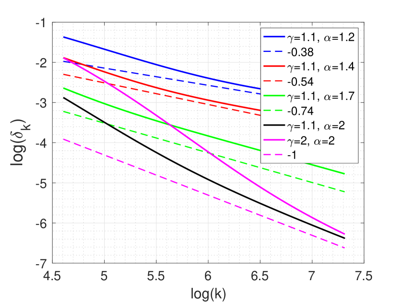
(a) $\tau=0$.

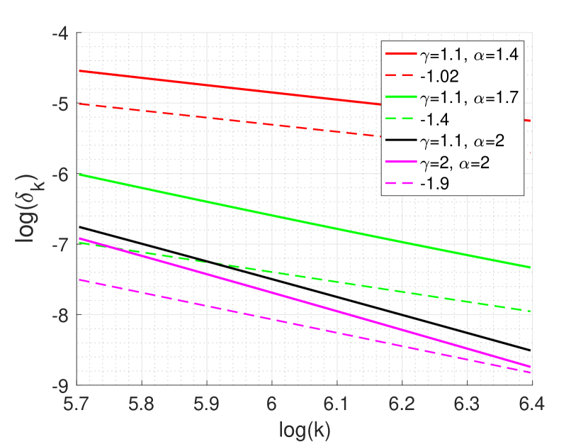
(b) $\tau=0.9$.

(c) $\tau=2$.

Figure 1: Behavior of the dynamics in (6) for $h(t)=t^{\beta}$, $\phi(t)=\sqrt{2\mu}\ t^{1/\alpha}$, $\tau\in\{0,0.9,2\}$, and different $\alpha,\beta$. Each solid line shows $\log(\delta_{k})$ as a function of $\log(k)$, for a given set of parameters and each dashed line shows the corresponding theoretical convergence rate of $\delta_{k}$ presented in Corollary 1. The numbers assigned to dashed lines indicate the slope of those lines. (a) and (b) verify the case corresponding to $\tau\leq\gamma/(4-\alpha-\gamma)$ and (c) verifies the case $\tau>\gamma/(4-\alpha-\gamma)$. Note that the distance between the dashed and solid lines is due to constant factors.

3.2 Sample complexity of SGD

The result of Corollary 1 suggests that by increasing the cost of the gradient estimator $b_{k}$ over the iterations, one can achieve a better iteration complexity of Algortihm 1. In particular, it improves with $\tau$ until it reaches the minimum $N={\cal O}\left(\epsilon_{f}^{-\frac{4-\alpha-\gamma}{\alpha}}\right)$ at $\tau=\frac{\gamma}{4-\alpha-\gamma}$ and does not change for larger values of $\tau$. However, we are merely interested in the iteration complexity in practice, since the computational cost at each iteration can be prohibitively large. A more adequate measure is the total computational cost (sample complexity) of the method. It is interesting whether increasing $b_{k}$ over the iterations may also result in a better sample complexity for finding an $\epsilon_{f}$-optimal solution, than for the constant choice, e.g., $b_{k}=1$. The following lemma shows the contrary.

Proposition 1.

Let the assumptions of Corollary 1 hold, $b_{k}=\Theta\left(k^{\tau}\right)$, $T=\Theta\left(1\right)$. Then the expected total computational cost (sample complexity) of Algorithm 1 is

$$\text{cost}:=T\cdot\sum_{k=0}^{K-1}b_{k}=\begin{cases}{\cal O}\left(\epsilon_{f}^{-\frac{4-\alpha}{\alpha}}\right)\qquad&\text{for }0\leq\tau\leq\frac{\gamma}{4-\alpha-\gamma},\\ {\cal O}\left(\epsilon_{f}^{-\frac{\left(4-\alpha-\gamma\right)\left(\tau+1\right)}{\alpha}}\right)\qquad&\text{for }\tau>\frac{\gamma}{4-\alpha-\gamma}.\end{cases}$$

The above result implies that increasing the cost of the gradient estimator with iterations does not improve the total sample complexity of Algorithm 1. Therefore, one can simply select $b_{k}=1$ ($\tau=0$) and obtain ${\cal O}\left(\epsilon_{f}^{-\frac{4-\alpha}{\alpha}}\right)$ sample complexity.

3.3 Tightness of rates in Corollary 1

In this section, we show that when $\tau=0$, the convergence rates presented in Corollary 1 are tight for the dynamic (6) describing the progress of SGD. More precisely, if there exists a function $f$ and a gradient estimator satisfying the assumptions in Corollary 1 such that its corresponding recursive inequality (6) is an equality, then its convergence rate, presented in Corollary 1 cannot be improved by any choices of stepsizes $\left\{\eta_{k}\right\}_{k\geq 0}$. Next proposition summarizes our results about the tightness of our convergence rates in Corollary 1.

Proposition 2.

Consider the following recursion

$$\delta_{k+1}=\delta_{k}+a\eta_{k}^{2}\cdot h\big{(}\delta_{k}\big{)}-\frac{\eta_{k}}{2}\phi^{2}(\delta_{k})+\frac{d\eta_{k}^{2}}{b_{k}},\quad\text{for all }k\geq 0,$$

where $a\geq 0$, $d>0$, $h(t)=t^{\beta}$ with $\beta\in(0,1]$, $\phi(t)=\sqrt{2\mu}t^{1/\alpha}$ with $\alpha\in[1,2]$, and $b_{k}=\Theta(1)$. Then $\delta_{k}={\Omega}(k^{-\frac{\alpha}{4-\alpha}})$ for any sequence of $\left\{\eta_{k}\right\}_{k\geq 0}$. Moreover, this rate is achieved by the choice $\eta_{k}=\Theta(k^{-\frac{1}{2-\alpha/2}})$.

4 Faster Rates with Variance Reduction

1:  Initialization: $\bar{x}_{0},\bar{g}_{0},K,\left\{\Lambda_{k}=\left(\eta_{k},T_{k},p_{k},b_{k},b_{k}^{\prime}\right):k=0,...,K-1\right\}$

2:  for $k=0,\ldots,K-1$ do

3:     $\left(x_{0},g_{0}\right)\leftarrow\left(\bar{x}_{k},\bar{g}_{k}\right)$

4:     $\left(\eta,p,b,b^{\prime}\right)\leftarrow\left(\eta_{k},p_{k},b_{k},b_{k}^{\prime}\right)$

5:     for $t=0,\ldots,T_{k}-1$ do

6:        $x_{t+1}=x_{t}-\eta g_{t}$

7:        Sample $\chi\sim\text{Bernoulli}(p)$

8:        if $\chi=1$ then

9:           $g_{t+1}=\frac{1}{b}\sum_{i=1}^{b}\nabla f_{\xi_{t+1}^{i}}(x_{t+1})$

10:        else

11:           $g_{t+1}=g_{t}+\frac{1}{b^{\prime}}\sum_{i=1}^{b^{\prime}}\nabla f_{\xi_{t+1}^{i}}(x_{t+1})-\frac{1}{b^{\prime}}\sum_{i=1}^{b^{\prime}}\nabla f_{\xi_{t+1}^{i}}(x_{t})$

12:     $\left(\bar{x}_{k+1},\bar{g}_{k+1}\right)\leftarrow\left(x_{t+1},g_{t+1}\right)$

13:  Return: $\bar{x}_{K}$

Algorithm 2 PAGER (PAGE with restarts)

To simplify the exposition of the results in this section, let us assume that $g_{k}(x_{t},\xi_{t})$ is constructed explicitly via mini-batching $g_{k}(x_{t},\xi_{t}):=\frac{1}{b_{k}}\sum_{i=1}^{b_{k}}\nabla f_{\xi_{t}^{i}}(x_{t}),$ where $\xi_{t}:=\left(\xi_{t}^{1},\ldots,\xi_{t}^{b_{k}}\right)$ is a random vector of independent entries, $\xi_{t}$ are independent for all iterations, $\tiny{\{\nabla f_{\xi_{t}^{i}}(x_{t})\}}_{i=1}^{b_{k}}$ are queries provided by an oracle such that $\mathbb{E}[\nabla f_{\xi_{t}^{i}}(x_{t})]=\nabla f(x_{t})$ and $\mathbb{E}[||\nabla f_{\xi_{t}^{i}}(x_{t})-\nabla f(x_{t})||^{2}]\leq\sigma^{2}$ for all $t\geq 0$. The variance of this estimator diminishes linearly in the size of the mini-batch $b_{k}$, i.e., $g_{k}(x_{t},\xi_{t})$ satisfies

Assumption 5 ($k$-BV, bounded variance).

Let Assumption 4 hold with $A=0$, $B=1$ and $C=\sigma^{2}$, i.e., ${\mathbb{E}}\left[\left\|g_{k}(x,\xi)-\nabla f(x)\right\|^{2}\right]\leq\frac{\sigma^{2}}{b_{k}}$.

Additionally, we assume that we have access to a gradient estimator $g_{k}^{\prime}(x,\xi)$, which satisfies the following

Assumption 6 (Average $\mathcal{L}$-smoothness (of order $k$)).

Let $g_{k}^{\prime}(x,\xi):=\frac{1}{b_{k}^{\prime}}\sum_{i=1}^{b_{k}^{\prime}}\nabla f_{\xi^{i}}(x)$ and $g_{k}^{\prime}(y,\xi):=\frac{1}{b_{k}^{\prime}}\sum_{i=1}^{b_{k}^{\prime}}\nabla f_{\xi^{i}}(y)$ be unbiased mini-batch estimators of the gradient of $f(\cdot)$ at points $x$ and $y$, respectively for shared stochasticity $\xi^{i}\sim\mathcal{D}$ for each $i=1,\dots,b_{k}^{\prime}$ and $\xi=(\xi^{1},\ldots,\xi^{b_{k}})$. Define $\widetilde{\Delta}(x,y):=g_{k}^{\prime}(x,\xi)-g_{k}^{\prime}(y,\xi)$. The average $\mathcal{L}$-smoothness (of order $k$) holds if there exists $\mathcal{L}\geq 0$ such that ${\mathbb{E}}\left[\left\|\widetilde{\Delta}(x,y)-\Delta(x,y)\right\|^{2}\right]\leq\frac{\mathcal{L}^{2}}{b_{k}^{\prime}}\left\|x-y\right\|^{2}\quad\text{for all }x,y\in\mathbb{R}^{d},$ where $\Delta(x,y):=\nabla f(x)-\nabla f(y)$.

Remark 1.

The Assumption 6 holds in several standard settings. For instance, if each $\nabla f_{\xi^{i}}(x)$ is Lipschitz with constant $\bar{L}$ (almost surely or on average), then Assumption 6 holds with $\mathcal{L}\leq\bar{L}$. Another example is when $f(\cdot)$ is of the form (2) and $b_{k}^{\prime}=n$, then $\mathcal{L}=0$.

4.1 PAGER – a new variance reduction for $\alpha$-PŁ objectives

We remark from the analysis of Algorithm 1 in Section 3 that merely playing with choice of $\eta_{k}$ and $b_{k}$ (chosen as polynomial functions of $k$) is not sufficient to improve the convergence, hence, we need to construct more sophisticated gradient estimator and reduce the variance using control variate. Now, we highlight the main algorithmic ingredients of our construction. First, let us describe the variance reduced estimator named PAGE, which will be the main building block for our Algorithm 2. PAGE was introduced and analyzed in [36] and is known to be optimal for finding a first order stationary point. Moreover, it is easy to implement and designed via a small modification to mini-batch SGD

$$g_{t+1}=\begin{cases}\frac{1}{b}\sum_{i=1}^{b}\nabla f_{\xi_{t+1}^{i}}(x_{t+1}),&\text{w.p.}\quad\ p,\\ g_{t}+\frac{1}{b^{\prime}}\sum_{i=1}^{b^{\prime}}\left(\nabla f_{\xi_{t+1}^{i}}(x_{t+1})-\nabla f_{\xi_{t+1}^{i}}(x_{t})\right),&\text{w.p.}\ 1-p,\end{cases}$$

where $p$ is a small probability and mini-batch sizes satisfy $b>b^{\prime}$.

However, while the method looks simple, the extension of its analysis to $\alpha$-PŁ functions faces several difficulties. Therefore, we introduce a new method, which we call PAGER (Algorithm 2) – a Probabilistic Average Gradient Estimator with parameter Restart. It takes as input the sequence of parameters $\left\{\Lambda_{k}:=\left(\eta_{k},T_{k},p_{k},b_{k},b_{k}^{\prime}\right):k=0,...,K-1\right\}$, where $T_{k}$ is the length of stage $k$, $\eta_{k},p_{k},b_{k},b_{k}^{\prime}$ step-size, probability, and batch-sizes at stage $k$. PAGER updates this sequence of parameters in the outer loop $k=0,\ldots,K-1$ and applies PAGE estimator with a fixed set of parameters in the inner loop $t=0,\ldots,T_{k}-1$. We will select $\left\{\Lambda_{k}\right\}_{k\geq 0}$ depending on the PŁ power $\alpha$ to capture the dependence on the geometry of the problem and establish fast rates for each $\alpha$ in settings (1) and (2).

4.2 Online case

We present convergence guarantees for Algorithm 2 in the setting (1) and defer its formal proof to Appendix C.

Theorem 2.

Let $f(\cdot)$ have the form (1) and satisfy Assumptions 1, 3 (with $\alpha\in[1,2)$), 5 and 6, let the sequences in Algorithm 2 be chosen as $b_{k}^{\prime}=\Theta\big{(}2^{\frac{(2-\alpha)k}{\alpha}}\big{)}$, $p_{k}=\Theta\big{(}2^{\frac{-(2-\alpha)k}{\alpha}}\big{)}$, $b_{k}=\Theta\big{(}2^{\frac{2k}{\alpha}}\big{)}$, $T_{k}=\Theta\big{(}2^{\frac{(2-\alpha)k}{\alpha}}\big{)}$, $\eta_{k}=\Theta\big{(}1\big{)}$. Then, for any $\epsilon_{f}>0$ Algorithm 2 returns a point $x$ with ${\mathbb{E}}\left[f(x)-f^{\star}\right]\leq\epsilon_{f}$ after $N:=\sum_{k=0}^{K-1}T_{k}={\cal O}\big{(}\kappa\epsilon_{f}^{-\frac{2-\alpha}{\alpha}}\big{)}$ iterations, where $\kappa=\nicefrac{{\mathcal{L}}}{{\mu}}$. The expected total computational cost (sample complexity) is ${\cal O}\left(\left(\frac{\sigma^{2}}{\mu}+\kappa^{2}\right)\epsilon_{f}^{-\frac{2}{\alpha}}\right)$.

Improvement over SGD.

Theorem 2 implies that PAGER improves the sample complexity of SGD from ${\cal O}\big{(}\epsilon_{f}^{-\frac{4-\alpha}{\alpha}}\big{)}$ to ${\cal O}\big{(}\epsilon_{f}^{-\frac{2}{\alpha}}\big{)}$ under $\alpha$-PŁ condition for the whole spectrum of parameters $\alpha\in[1,2)$. In the case $\alpha=1$, which holds in many interesting applications (see Appendix A for examples), this leads to ${\cal O}\big{(}\epsilon_{f}^{-2}\big{)}$ sample complexity compared to the best known ${\cal O}\big{(}\epsilon_{f}^{-3}\big{)}$ for SGD.

Relation to convex optimization and last iterate convergence.

As a consequence of our analysis we obtain the optimal sample complexity for convex stochastic optimization under the additional assumption that the iterates of the method remain bounded, i.e., $\left\|x_{t}-x^{\star}\right\|^{2}\leq D$ for all $t\geq 0$, where $x^{\star}\in\operatorname*{arg\,min}_{x}f(x)$. For $1$-PŁ objectives, PAGER has ${\cal O}\left(\epsilon_{f}^{-2}\right)$ sample complexity. Since the iterates of the algorithm are bounded, convexity $\langle\nabla f(x),x-x^{\star}\rangle\geq f(x)-f(x^{\star})$ implies $1$-PŁ with $\mu=\frac{1}{2D}$. This observation implies convergence of PAGER for convex objectives with ${\cal O}\left(\epsilon_{f}^{-2}\right)$ sample complexity, which is known to be non-improvable for convex stochastic optimization [42].

Moreover, we highlight that this result holds for the last iterate of PAGER, while the standard analysis of first order methods for convex functions guarantees convergence for the average iterate [31]. The last iterate convergence for convex objectives was only recently established for SGD by following an involved analysis with a careful control of iterates via suffix-averaging scheme [20].

4.3 Finite sum case

Let $f(\cdot)$ have the finite sum form (2). Then we obtain the following result.

Theorem 3.

Let $f(\cdot)$ have the form (2) and satisfy Assumptions 1, 3 (with $\alpha\in[1,2)$) and 6, let the sequences be chosen as $p_{k}=\frac{1}{n+1}$, $b_{k}^{\prime}=1$, $b_{k}=n$, $T_{k}=\Theta\big{(}2^{\frac{(2-\alpha)k}{\alpha}}\big{)}$, $\eta_{k}=\Theta\big{(}1\big{)}$. Then, for any $\epsilon_{f}>0$, Algorithm 2 returns a point $x$ with ${\mathbb{E}}\left[f(x)-f^{\star}\right]\leq\epsilon_{f}$ after $N:=\sum_{k=0}^{K-1}T_{k}={\cal\widetilde{O}}\big{(}n+\sqrt{n}\kappa\epsilon_{f}^{-\frac{2-\alpha}{\alpha}}\big{)}$ iterations, where $\kappa=\nicefrac{{\mathcal{L}}}{{\mu}}$ The expected total computational cost (sample complexity) is ${\cal\widetilde{O}}\big{(}n+\sqrt{n}\kappa\epsilon_{f}^{-\frac{2-\alpha}{\alpha}}\big{)}$.

The proof is deferred to Appendix C. Theorem 3 quantifies the improvement of PAGER over GD in the finite sum setting in terms of $n$ and over SGD in terms of $\epsilon_{f}$, see Table 1 for comparison. Recall that GD has sample complexity ${\cal O}\big{(}n\kappa\epsilon_{f}^{\frac{-(2-\alpha)}{\alpha}}\big{)}$. When $n$ is large, we get the improvement of order $\sqrt{n}$. Notice that in the limit $\alpha\rightarrow 2$, it matches the best known result for $2$-PŁ objectives [36].

5 Conclusion

We analyzed the complexity of SGD when the objective satisfies global KŁ inequality and the queries from stochastic gradient oracle satisfy weak expected smoothness. We introduced a general framework for this analysis which resulted in a sample complexity of $\mathcal{O}(\epsilon^{-(4-\alpha)/\alpha})$ for SGD with objectives satisfying $\alpha$-PŁ condition. We also demonstrated the tightness of this rate under the specific choice of stepsizes. Last but not least, we developed a modified SGD with variance reduction and restarting (PAGER), which improves the sample complexity of SGD for the whole spectrum of parameters $\alpha\in[1,2)$ and achieves the optimal rate for the important case of $1$-PŁ objectives.

Appendix

Appendix A Examples

A.1 $\alpha$-PŁ Functions

In this section, we provide some examples and applications of global KŁ functions. Particularly, we focus on the class of $\alpha$-PŁ functions with $\alpha\in[1,2]$. We start with simple one dimensional functions.

Example 1.

Consider $f(x)=c\cdot|x|^{q}$, where $q>1$, $c>0$. $f(x)$ satisfies Assumption 3 with $\alpha=\frac{q}{q-1}$ and $\mu=\frac{c^{\nicefrac{{2}}{{q}}}q^{2}}{2}$.

Example 2.

Consider $f(x)=\frac{e^{x}+e^{-x}}{2}-1$. $f(x)$ satisfies Assumption 3 with $\alpha=1$ and $\mu=\nicefrac{{1}}{{2}}$.

Example 3.

Consider $f(x)=cosh(x)+8\cdot cosh(sin(x))-9$, where $cosh(x)=\nicefrac{{(e^{x}+e^{-x})}}{{2}}$. The derivative is $f^{\prime}(x)=sinh(x)+8\cdot cos(x)\cdot sinh(sin(x))$ and $|f^{\prime}(x)|\geq 10^{-2}\cdot f(x)$ for all $x$. Then $f(x)$ satisfies Assumption 3 with $\alpha=1$ and $\mu=5\cdot 10^{-5}$.

Note that the functions in Example 1 and Example 2 are convex, whereas the function in Example 3 is nonconvex.

The following proposition shows that KŁ property is preserved under some operators such as direct addition.

Proposition 3.

Let $f(\cdot)$ be a separable function, i.e., $f(x):=\frac{1}{n}\sum_{i=1}^{n}f_{i}(x_{i})$, where $x=(x_{1},\dots,x_{n})$, $x_{i}\in\mathbb{R}^{d_{i}}$, $\sum_{i=1}^{n}d_{i}=d$. Let each $f_{i}(\cdot)$ satisfy KŁ inequality (Assumption 2) with $\phi_{i}(t)$. Then $f(\cdot)$ also satisfies KŁ inequality with $\phi(t):=\frac{1}{\sqrt{n}}\min_{1\leq i\leq n}\phi_{i}(t)$.

Proof.

By separability and KŁ condition we have

$$\left\|\nabla f(x)\right\|^{2} = \sum_{i=1}^{n}\frac{1}{n^{2}}\left\|\nabla f_{i}(x_{i})\right\|^{2}$$ (9)

$$\geq \sum_{i=1}^{n}\frac{1}{n^{2}}\phi_{i}^{2}\left(f_{i}(x_{i})-f_{i}^{inf}\right)$$

$$\overset{(i)}{\geq} \frac{1}{n}\sum_{i=1}^{n}\phi^{2}\left(f_{i}(x_{i})-f_{i}^{inf}\right)$$

$$\overset{(ii)}{\geq} \phi^{2}\left(\frac{1}{n}\sum_{i=1}^{n}f_{i}(x_{i})-f_{i}^{inf}\right)$$

$$\overset{(iii)}{\geq} \phi^{2}\left(f(x)-f^{inf}\right),$$

where $(i)$ holds by definition of $\phi(t)$, $(ii)$ is due to convexity of $\phi(t):=\frac{1}{\sqrt{n}}\min_{1\leq i\leq n}\phi_{i}(t)$ and Jensen’s inequality and $(iii)$ follows from $\frac{1}{n}\sum_{i=1}^{n}\inf_{x_{i}}f_{i}(x_{i})\leq\inf_{x}\frac{1}{n}\sum_{i=1}^{n}f_{i}(x)$ for any $x=(x_{1},\dots,x_{n})$. ∎

The above Proposition 3 implies, in particular, that if we have a separable function $f(x)=\sum_{i=1}^{n}f_{i}(x_{i})$ and each $f_{i}(x_{i})$ is $1$-PŁ with $\mu_{i}$, $i=1,\ldots,n$, then $f(x)$ satisfies $1$-PŁ with $\mu=\frac{\mu_{min}}{n}$ .

Example 4.

Consider $f(x,y)=cosh(x)+8\cdot cosh(sin(x))+0.5\cdot cosh(y)+2.5\cdot cosh(sin(y))-12$. This function of two variables satisfies Assumption 3 with $\alpha=1$ and $\mu=5\cdot 10^{-5}$.

Now we list several problems which occur in applications and satisfy $\alpha$-PŁ with $\alpha=1$.

Example 5 (Policy gradient optimization in RL).

Consider a Markov Decision Process (MDP) $M=\{\mathcal{S},\mathcal{A},\mathcal{P},\mathcal{R},\gamma,\rho\}$, where $\mathcal{S}$ is a state space; $\mathcal{A}$ is an action space; $\mathcal{P}$ is a transition model, where $\mathcal{P}(s^{\prime}|s,a)$ is the transition density to state $s^{\prime}$ from a given state $s$ under a given action $a$; $\mathcal{R}=\mathcal{R}(s,a)$ is the bounded reward function for state-action pair $(s,a)$; $\gamma\in[0,1)$ is the discount factor; and $\rho$ is the initial state distribution. The behavior of the agent in MDP is characterized by the parametric policy $\pi_{\theta}(a|s)$ over $\mathcal{S}\times\mathcal{A}$, which denotes the probability of taking action $a$ at the state $s$. The policy $\pi_{\theta}$ is assumed to be differentiable with respect to parameter $\theta\in\mathbb{R}^{d}$. Let $\tau=\left\{s_{t},a_{t}\right\}_{t\geq 0}$ be a trajectory generated by the policy $\pi_{\theta}$ and it is distributed according to distribution $\tau\sim p(\tau|\pi_{\theta})$. The expected return of the policy $\pi_{\theta}$ is defined by

$$J\left({\theta}\right):=\mathbb{E}_{\tau}\left[\sum_{t=0}^{\infty}\gamma^{t}\mathcal{R}\left(s_{t},a_{t}\right)\right].$$

The goal of policy-based methods is to find $\theta$ which maximizes the expected return $\theta^{\star}\in\operatorname*{arg\,max}_{\theta}J(\theta)$. It was recently shown that the above objective satisfies $1$-PŁ assumption

$$\left\|\nabla J(\theta)\right\|\geq\sqrt{2\mu}\left(J^{\star}-J(\theta)\right)\qquad\text{for all }\theta\in\mathbb{R}^{d}$$

under the standard assumptions on $\pi_{\theta}$ and $\rho$ such as non-degenerate Fisher matrix and transferred compatible function approximation error [41, 1, 56].

Example 6 (Operations management problems).

In applications such as supply chain or revenue management [14], problems can often be formulated as

$$\min_{x\in\mathcal{X}}F(x):={\mathbb{E}}\left[\phi(x\wedge\xi)\right],$$ (10)

where $\mathcal{X}$ is a convex compact subset of $\mathbb{R}^{d}$, $\xi$ is a random vector, $\wedge$ denotes a component-wise minimum and $\phi(\cdot)$ is convex. As a result, $F(\cdot)$ becomes non-convex. On the other hand, such problem often admits a convex reformulation

$$\min_{y\in\mathcal{Y}}G(y):=F(g^{-1}(y)),$$ (11)

where $g(x)={\mathbb{E}}\left[x\wedge\xi\right]$ and function $G(\cdot)$ is convex. Suppose $g:\mathcal{X}\rightarrow\mathcal{Y}$ is a bijective differentiable map with $\nabla g(x)\succeq\lambda I$, $\lambda>0$ for all $x\in\mathcal{X}$, then function $F(\cdot)$ satisfies $1$-PŁ condition. This is because: for any $x$ with $g(x)=y$,

$$F(x)-F(x^{\star}) = G(y)-G(y^{\star})$$

$$\leq \langle\nabla G(y),y-y^{\star}\rangle$$

$$\leq \left\|\nabla G(y)\right\|\left\|y-y^{\star}\right\|$$

$$= \left\|\nabla g^{-1}(y)\nabla F(x)\right\|\left\|y-y^{\star}\right\|$$

$$\leq \frac{D_{\mathcal{Y}}}{\lambda}\left\|\nabla F(x)\right\|,$$

where $D_{\mathcal{Y}}$ is the diameter of the set $\mathcal{Y}$. Therefore, $F(\cdot)$ is $1$-PŁ with $\mu=\frac{1}{2}\frac{\lambda^{2}}{D_{\mathcal{Y}}^{2}}$.

Remark 2.

Note that even though the problem in Example 6 satisfies $1$-PŁ condition, our theory developed in this work is not directly applicable to solve this problem The reason is that this problem has a compact constraint and therefore requires an appropriate generalization of PŁ condition, e.g., using the notion of gradient mapping or the subgradient of the indicator function of the set $\mathcal{X}$, see [29] for examples. However, our theory becomes applicable for this problem if we additionally assume that the solution of (10) lies in the interior of $\mathcal{X}$ and all the iterates $\left\{x_{t}\right\}_{t\geq 0}$ generated by the method remain in the interior of $\mathcal{X}$.

A.2 KŁ Functions

Example 7.

A commonly used type of loss function in machine learning applications is a squared cross entropy (CE), it is given by

$$\ell(x,y):=\sum_{i}y_{i}\log\Big{(}\frac{e^{x_{i}}}{\sum_{j}e^{x_{j}}}\Big{)}^{2}.$$

Under such loss function, it is known [51] that KŁ condition holds with corresponding function $\phi(t)=\min\{t,\sqrt{t}\}$. This is function is both positive and $\phi(t)^{2}$ is convex. Next, we apply the result of Theorem 1 to obtain the convergence rate of SGD for this type of loss functions assuming the stochastic gradient estimator satisfying Assumption 4 with $h(t)=t$. First step is to obtain the stationary point $r(\eta)$ using Equation (7).

$$2a\eta^{2}t+2\frac{d\eta^{2}}{b}=\eta\big{(}\min\{t,\sqrt{t}\}\big{)}^{2}.$$

It is straightforward to see that for small enough $\eta$, the stationary point is smaller than 1. In this case, $\min\{t,\sqrt{t}\}$ is $t$. Therefore, we are in the setting of Corollary 1 with $\alpha=1,\beta=1$, and $\tau=0$. This implies that the interation (and sample) complexity of SGD is of the order $\mathcal{O}(\epsilon_{f}^{-3})$. Moreover, if $A$ in Assumption 4 is zero, using a similar argument and the result of Theorem 2, one can derive that PAGER give us $\mathcal{O}(\epsilon_{f}^{-2})$ sample complexity.

To illustrate the generality of the result of Theorem 1, next we present the convergence rate of SGD for objective functions that satisfy the global KŁ condition with $\phi(t)=\sqrt{t\log(t+1)}$ under Assumption 4 with $h(t)=\log(1+t)$.

Example 8.

Consider the scenario in which the objective function satisfies the global KŁ condition with $\phi(t)=\sqrt{t\log(t+1)}$ and a stochastic gradient estimator satisfies Assumption 4 with $h(t)=\log(1+t)$. In this case, Equation (7) becomes

$$2a\eta^{2}\log(1+t)+2\frac{d\eta^{2}}{b}=\eta t\log(1+t).$$

Defining $u:=\log(t+1)$ yields

$$\eta\big{(}2au+2\frac{d}{b}\big{)}=(e^{u}-1)u\approx(u+\frac{u^{2}}{2})u.$$

The last approximation is true since for small enough $\eta$, $u$ is less than one. Solving the above cubic equation leads to a solution that is of the order $u=\Theta(\sqrt{\eta})$ or equivalently $r(\eta)=\Theta(\exp(\sqrt{\eta})-1)$. Note that for small enough $\eta\ll 1$, we have $\Theta(\exp(\sqrt{\eta})-1)=\Theta(\sqrt{\eta}+\eta)=\Theta(\sqrt{\eta})$, i.e., $\nu=0.5$. To obtain $\zeta$ in Theorem 1, we use Equation (8) which leads to

$$1+\frac{a\eta^{2}_{k}}{1+r(\eta_{k})}-\frac{\eta_{k}}{2}\Big{(}\frac{r(\eta_{k})}{1+r(\eta_{k})}+\log(1+r(\eta_{k}))\Big{)}$$

$$=1+\frac{a\eta^{2}_{k}}{1+\sqrt{\eta_{k}}}-\frac{\eta_{k}}{2}\Big{(}\frac{\sqrt{\eta_{k}}}{1+\sqrt{\eta_{k}}}+\log(1+\sqrt{\eta_{k}})\Big{)}=1-\omega_{k}k^{-1},$$

In order to have the above equality, we can have $\eta_{k}=\Theta(k^{-1})$. Finally, the result of Theorem 1 yields $\delta_{k}=\mathcal{O}(k^{-\zeta\nu})=\mathcal{O}(k^{-0.5})$.

Appendix B Proofs for Section 3

B.1 Proof of Lemma 1

Lemma 1. Under Assumptions 1, 2, and 4 with constant cost, i.e., $b:=b_{k}$, we obtain

$$\delta_{t+1}\leq\delta_{t}+a\eta^{2}\cdot h\big{(}\delta_{t}\big{)}-\frac{\eta}{2}\phi^{2}(\delta_{t})+\frac{d\eta^{2}}{b},$$

where $\delta_{t}:={\mathbb{E}}\left[f(x_{t})-f^{\star}\right]$, $a:=LA$, $d:=\frac{LC}{2}$, $\eta:=\eta_{k}$.

Proof.

Let $\{x_{0},x_{1},x_{2},...\}$ denote the sequence of points that are obtained from SGD. From the L-smoothness assumption, we obtain

$$f(x_{t+1})\leq f(x_{t})-\eta\langle\nabla f(x_{t}),g_{k}(x_{t},\xi_{t})\rangle+\frac{L}{2}||x_{t+1}-x_{t}||^{2}.$$

Taking the conditional expectation of both side of the above inequality given $x_{t}$ yields

$$\mathbb{E}[f(x_{t+1})-f(x_{t})|x_{t}]\leq-\eta\mathbb{E}\big{[}\langle\nabla f(x_{t}),g_{k}(x_{t},\xi_{t})\rangle|x_{t}\big{]}+\frac{L}{2}\eta^{2}\mathbb{E}\big{[}||g_{k}(x_{t},\xi_{t})||^{2}|x_{t}\big{]}.$$

Using Assumption 4 and the fact that oracle’s queries are unbiased, we obtain

$$\mathbb{E}[f(x_{t+1})\!-\!f(x_{t})|x_{t}]\leq LA\eta^{2}\cdot h\big{(}f(x_{t})\!-\!f^{*}\big{)}-\eta(1-\!\frac{L}{2}\eta B)\cdot\phi^{2}\big{(}f(x_{t})\!-\!f^{*}\big{)}+\frac{L}{2}\eta^{2}\frac{C}{b},$$

where $b=b_{k}$ denotes the cost of gradient $g_{k}$. Since the choice of learning rate is ours, we select it such that $(1-\frac{L}{2}\eta B)\geq\frac{1}{2}$. Using Assumption 2 for points around the optimum point $x^{*}$, we obtain

$$\mathbb{E}[\varrho_{t+1}|x_{t}]-\varrho_{t}\leq a\eta^{2}\cdot h\big{(}\varrho_{t}\big{)}-\frac{\eta}{2}\phi^{2}(\varrho_{t})+\frac{d\eta^{2}}{b},$$

where $\varrho_{t}:=f(x_{t})-f^{*}$, $a:=LA$, and $d:=\frac{LC}{2}$. Let $\delta_{t}=\mathbb{E}[\varrho_{t}]$. Using the fact $h(t)$ is concave and $\phi^{2}$ is convex, and Jensen’s inequality, we obtain the result. ∎

B.2 Proof of Theorem 1

We first prove the following technical lemma.

Lemma 2.

Consider a series $\{r_{t}\}_{t\geq 0}$ that for every integer $T>0$ satisfies the following inequality

$$r_{t}\leq\prod_{i=1}^{k}(1-a_{i}i^{-1})^{T}r_{0}+\mathcal{O}(k^{-b}),$$

where $t=kT$ and $a<a_{i}<A\leq 1$ for some positive constants $a$ and $A$ and all $i$. Then, there exists $T$ such that $r_{t}=\mathcal{O}(t^{-b})$.

Proof.

Using the fact that $a_{i}$s are bounded and $1-x\leq\exp(-x)$, we obtain

$$\prod_{i=1}^{k}(1-a_{i}i^{-1})^{T}\leq\exp\big{(}-aT\sum_{i=1}^{k}i^{-1}\big{)}\leq(k+1)^{-aT}.$$

In the above inequality, we used $\sum_{i=1}^{k}i^{-1}\geq\int_{1}^{k+1}x^{-1}dx=\log(k+1)$. Selecting $T=\lceil b/a\rceil$ will imply the result. ∎

Theorem 1. Suppose there exist $\nu,\{\omega_{j}\}_{j\geq 0}$, and $\zeta\geq 0$ such that $\eta_{k}=\Theta(k^{-\zeta})$, $r(\eta_{k})=\Theta(k^{-\zeta\nu})$, $|1-\omega_{k}|<1$, and

$$1+a\eta^{2}_{k}h^{\prime}\big{(}r(\eta_{k})\big{)}-\eta_{k}\phi^{\prime}\big{(}r(\eta_{k})\big{)}\phi\big{(}r(\eta_{k})\big{)}=1-\omega_{k}k^{-1}.$$

Then, $\delta_{k}=\mathcal{O}(k^{-\zeta\nu})$ and the iteration complexity of Algorithm 1 is $\mathcal{O}(\epsilon_{f}^{-1/(\zeta\nu)})$.

Proof.

Suppose, we are in the $k$ iteration of the outer-loop of Algorithm 1. Using Lemma 1 and the definition of $r(\eta)$ in (7), we have

$$\delta_{t+1}\leq\delta_{t}+a\eta_{k}^{2}\Big{(}h\big{(}\delta_{t}\big{)}-h\big{(}r(\eta_{k})\big{)}\Big{)}-\frac{\eta_{k}}{2}\Big{(}\phi^{2}(\delta_{t})-\phi^{2}\big{(}r(\eta_{k})\big{)}\Big{)}.$$

By defining $y_{t}:=\delta_{t}-r(\eta_{k})$ and using the concavity of functions $h(\cdot)$ and $-\phi^{2}(\cdot)$, we obtain

$$y_{t+1} \leq y_{t}\Big{(}1+a\eta_{k}^{2}h^{\prime}\big{(}r(\eta_{k})\big{)}-\eta\phi^{\prime}\big{(}r(\eta_{k})\big{)}\phi\big{(}r(\eta_{k})\big{)}\Big{)}.$$

Given the assumption in Theorem 1, we have

$$y_{t+1}\leq y_{t}\big{(}1-\omega_{k}k^{-1}\big{)}.$$

Recall that $k$ corresponds to the index of the outer-loop. After $t$ iterations of the inner-loop (in which index $k$ is fixed), we obtain

$$y_{t}\leq y_{0}\big{(}1-\omega_{k}k^{-1}\big{)}^{t}.$$ (12)

This shows the rate at which the inner-loop of Algorithm 1 (lines 4-5) converges to point $x$, where $r(\eta_{k})=f(x)-f^{*}$. Based on Equation (12), after setting $\eta=\eta_{1}$ and $T_{1}$ rounds of the inner-loop, we obtain

$$y_{T_{1}}\leq y_{0}\big{(}1-\omega_{1}\big{)}^{T_{1}}\Rightarrow\delta_{T_{1}}\leq y_{0}\big{(}1-\omega_{1}\big{)}^{T_{1}}+r(\eta_{1}).$$

Continuing this process, after updating $\eta=\eta_{2}$ and going through the inner-loop for another $T_{2}$ iterations imply

$$y_{T_{1}+T_{2}}\leq(\delta_{T_{1}}-r(\eta_{2}))\big{(}1-\frac{\omega_{2}}{2}\big{)}^{T_{2}}\Rightarrow\delta_{T_{1}+T_{2}}\leq\big{(}y_{0}\big{(}1-\omega_{1}\big{)}^{T_{1}}+r(\eta_{1})-r(\eta_{2})\big{)}\big{(}1-\frac{\omega_{2}}{2}\big{)}^{T_{2}}+r(\eta_{2}).$$

The above inequality is because before starting the inner-loop for the second round, the initial point for $y$ is $y_{T_{1}}:=\delta_{T_{1}}-r(\eta_{2})$. Using induction and after $k$ rounds of outer-loop, we obtain

$$\delta_{t} \leq\prod_{i=1}^{k}\big{|}1-\frac{\omega_{i}}{i}\big{|}^{T_{i}}y_{0}+\prod_{i=1}^{k}\big{|}1-\frac{\omega_{i}}{i}\big{|}^{T_{i}}\left(\sum_{j=1}^{k-1}\frac{r(\eta_{j})-r(\eta_{j+1})}{\prod_{i^{\prime}=1}^{j}\big{(}1-\frac{\omega_{i^{\prime}}}{i^{\prime}}\big{)}^{T_{i^{\prime}}}}\right)+r(\eta_{k})$$

$$=\prod_{i=1}^{k}\big{|}1-\frac{\omega_{i}}{i}\big{|}^{T_{i}}y_{0}+\sum_{j=1}^{k-1}\big{(}r(\eta_{j})-r(\eta_{j+1})\big{)}\prod_{i=j+1}^{k}\big{|}1-\frac{\omega_{i}}{i}\big{|}^{T_{i}}+r(\eta_{k})$$

where $t=\sum_{j}T_{j}$. In Algorithm 1, $T_{i}$ are selected to be $T$. Next, using Lemma 2, we show there exist a positive constant $T$ such that $\delta_{t}=\mathcal{O}(t^{-\nu\zeta})$. Following the proof of Lemma 2, we have

$$\delta_{t} \leq\prod_{i=1}^{k}\big{|}1-\frac{\omega_{i}}{i}\big{|}^{T}y_{0}+\sum_{j=1}^{k-1}\big{(}r(\eta_{j})-r(\eta_{j+1})\big{)}\prod_{i=j+1}^{k}\big{|}1-\frac{\omega_{i}}{i}\big{|}^{T}+r(\eta_{k})$$

$$\leq(k+1)^{-\omega T}y_{0}+\sum_{j=1}^{k-1}\big{(}r(\eta_{j})-r(\eta_{j+1})\big{)}\left(\frac{j+1}{k+1}\right)^{\omega T}+r(\eta_{k}),$$

where $t=kT$ and $\omega=\min_{i}\omega_{i}$. Let $b:=\nu\zeta$ and $T:=\lceil(b+1)/\omega\rceil$. Since $r(\eta)=\Theta(\eta^{\nu})$ and $\eta_{j}=\Theta(j^{-\zeta})$, then there exists a constant $C>0$ such that

$$\delta_{t} \leq(k+1)^{-\omega T}y_{0}+C\sum_{j=1}^{k-1}\big{(}j^{-b}-(j+1)^{-b}\big{)}\left(\frac{j+1}{k+1}\right)^{\omega T}+\mathcal{O}(k^{-b})$$

$$\leq\mathcal{O}(k^{-b})+\frac{C}{(k+1)^{b+1}}\sum_{j=1}^{k-1}\Big{(}(1+\frac{1}{j})^{b}-1\Big{)}(j+1)+\mathcal{O}(k^{-b}).$$

Using $(1+x)^{b}-1\leq bx/(1-bx)$ for $x<1/b$ and $b\geq 0$, we obtain

$$\delta_{t} \leq\mathcal{O}(k^{-b})+\frac{C^{\prime}}{(k+1)^{b+1}}+\frac{Cb}{(k+1)^{b+1}}\sum_{j>b}^{k-1}\frac{j+1}{j-b}+\mathcal{O}(k^{-b})=\mathcal{O}(k^{-b}).$$

where $C^{\prime}\geq 0$ is a constant corresponding to the part of the summation for $j\leq b$. The result follows from the fact that $k=t/T$ and $T$ is a constant. ∎

B.3 Proof of Corollary 1

Corollary 1. Consider a special case of Assumption 4 with $h(t)=t^{\beta}$ and $b_{k}=k^{\tau}$, where $\beta\in(0,1]$ and $\tau\geq 0$. Suppose the objective function $f$ satisfies Assumptions 1 and 3. Let $\gamma:=\alpha\beta$. Then, for any $\epsilon_{f}>0$, Algorithm 1 returns a point $x$ with ${\mathbb{E}}\left[f(x)-f^{\star}\right]\leq\epsilon_{f}$ after $N:=K\cdot T$ iterations.
i) When $\gamma=2$ ($\alpha=2$ and $\beta=1$), we have

$$N=\mathcal{O}(\epsilon_{f}^{-\frac{1}{1+\tau}}),\ \text{with}\ \eta_{k}=\Theta(k^{-1}).$$

ii) When $\gamma<2$, we have

$$N=\mathcal{O}\big{(}\epsilon_{f}^{-\frac{4-\alpha}{\alpha(\tau+1)}}\big{)}\ \text{with}\ \eta_{k}=\Theta(k^{-\frac{\tau+1}{2-\alpha/2}+\tau})\ \text{if}\ \tau\leq\frac{\gamma}{4-\alpha-\gamma},and$$

$$N=\mathcal{O}\big{(}\epsilon_{f}^{-\frac{4-\alpha-\gamma}{\alpha}}\big{)}\ \text{with}\ \eta_{k}=\Theta(k^{-\frac{2-\gamma}{4-\alpha-\gamma}})\ \text{if}\ \tau>\frac{\gamma}{4-\alpha-\gamma}.$$

Proof.

Using the result of Theorem 1, we need to specify the constants $\nu$ and $\zeta$. To do so, we first characterize the stationary point for the special setting of this corollary. Equation (7) becomes

$$a\eta\cdot t^{\beta}+\frac{d\eta}{b}=\mu t^{2/\alpha}.$$ (13)

Let $\gamma:=\alpha\beta$ and define the following function

$$H_{\eta}(t):=a\eta^{2}t^{\beta}-\mu\eta t^{\frac{2}{\alpha}}+\frac{d\eta^{2}}{b}.$$

Next, we either find $r(\eta)$ exactly or bound it. Depending on whether $\gamma$ is less than or equal to $2$, the analysis of $H_{\eta}(t)=0$ is different. We study each case separately.

I) $\gamma=2$ (or $\beta=1$ and $\alpha=2$): In this case, we can find $r(\eta)$ exactly and it is given by

$$r(\eta)=\frac{\frac{d\eta}{b}}{\mu-a\eta}=\Theta\left(\frac{\eta}{b}\right)=\Theta\big{(}k^{-\tau}\eta\big{)}.$$

Note that in the above expression, we used the fact that $b_{k}=\Theta(k^{\tau})$. Next is to find the parameters in Theorem 1. To do so, from Equation 8 with $h(t)=t$ and $\phi(t)=\sqrt{2\mu t}$, we have

$$1+a\eta^{2}_{k}h^{\prime}\big{(}r(\eta_{k})\big{)}-\eta_{k}\phi^{\prime}\big{(}r(\eta_{k})\big{)}\phi\big{(}r(\eta_{k})\big{)}=1+a\big{(}\Theta(k^{-\zeta})\big{)}^{2}-\mu\Theta(k^{-\zeta})=1-\omega_{k}k^{-1}.$$

In order to have the above equality, we should have $\zeta=1$. Now, suppose that $\tau\geq 0$, then $r(\eta)=\Theta(k^{-(1+\tau)})$ and based on Theorem 1, we obtain the convergence rate of $\mathcal{O}(k^{-(1+\tau)})$ for $\delta_{k}$.

II) $0\leq\gamma<2$: In this case, we find lower and upper bound for $r(\eta)$. To this end, consider the following point for some constant $S$,

$$t_{0}:=\left(\frac{\frac{d\eta}{b}+S\frac{\eta}{b}}{\mu}\right)^{\frac{\alpha}{2}}=\Theta\left(\left(\frac{\eta}{b}\right)^{\frac{\alpha}{2}}\right).$$

For this point, we have

$$H_{\eta}(t_{0})=a\frac{\eta^{2+\frac{\gamma}{2}}}{b^{\frac{\gamma}{2}}}\Big{(}\frac{d+S}{\mu}\Big{)}^{\frac{\gamma}{2}}-S\frac{\eta^{2}}{b}.$$

For $S=0$, $H_{\eta}(t_{0})>0$. On the other hand, if $\eta=\Theta(k^{-\zeta})$ and $b_{k}=\Theta(k^{\tau})$, then for $(\tau+\zeta)\frac{\gamma}{2}\geq\tau$ and large enough $S$, we have $H_{\eta}(t_{0})<0$. This implies

$$r(\eta)=\Theta\left(\left(\frac{\eta}{b}\right)^{\frac{\alpha}{2}}\right).$$

Next is to check whether (8) holds for $\eta_{k}=\Theta(k^{-\zeta})$, $b_{k}=\Theta(k^{\tau})$, $h(t)=t^{\beta}$, and $\phi(t)=\sqrt{2\mu}t^{2/\alpha}$, i.e.,

$$1+a\beta\big{(}\Theta(k^{-\zeta})\big{)}^{2}\Big{(}\Theta(k^{-(\zeta+\tau)\alpha/2})\Big{)}^{\beta-1}-\frac{2\mu}{\alpha}\Theta(k^{-\zeta})\Big{(}\Theta(k^{-(\zeta+\tau)\alpha/2})\Big{)}^{2/\alpha-1}=1-\omega_{k}k^{-1}.$$

The order of the first term is $\mathcal{O}(k^{-(2\zeta+(\zeta+\tau)\alpha(\beta-1)/2)})$ and the order of the second term is $\mathcal{O}(k^{-(\zeta+(\zeta+\tau)\alpha(2/\alpha-1)/2)})$. In order for the above expression to hold, we should have

$$\zeta+(\zeta+\tau)\alpha(2/\alpha-1)/2\leq 2\zeta+(\zeta+\tau)\alpha(\beta-1)/2,$$ (14)

and

$$\zeta+(\zeta+\tau)\alpha(2/\alpha-1)/2\leq 1.$$ (15)

Inequality (14) implies $\gamma\zeta\geq(2-\gamma)\tau$ and inequality (15) leads to $\zeta<\frac{\tau+1}{2-\alpha/2}-\tau$. See Figure 2 for an example of the region $(\zeta,\tau)$ for which both (14) and (15) hold.

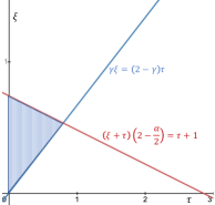
Figure 2: An illustration of the region $(\tau,\zeta)$ that ensures both (14) and (15) hold. This is the highlighted area. Within this region, the maximum $\gamma$ is at the red line. In this figure $\gamma=1.2,\alpha=1.3$, and $\beta=1.2/1.3=0.92$.

Putting everything together, we obtain

$$\text{If}\ \tau\leq\frac{\gamma}{4-\alpha-\gamma},\ \text{then}\ \delta_{k}=\mathcal{O}(k^{-\frac{\alpha(\tau+1)}{4-\alpha}}),\quad\text{with}\quad\eta_{k}=\Theta(k^{-\frac{\tau+1}{2-\alpha/2}+\tau}).$$

Note that $\frac{\gamma}{4-\alpha-\gamma}$ is the intersection point of two lines. For $\tau>\frac{\gamma}{4-\alpha-\gamma}$, the dynamic is equivalent to

$$\delta_{t+1}\leq\delta_{t}+a\eta^{2}\cdot\delta_{t}^{\beta}-\eta\mu\delta_{t}^{\frac{2}{\alpha}},$$ (16)

with the stationary point $r(\eta)=\big{(}a\eta/\mu\big{)}^{\frac{\alpha}{2-\gamma}}$. Following the steps similar to the previous case, we get the following equation

$$1+a\beta\big{(}\Theta(k^{-\zeta})\big{)}^{2}\Big{(}\Theta(k^{-\zeta\frac{\alpha}{2-\gamma}})\Big{)}^{\beta-1}-\frac{2\mu}{\alpha}\Theta(k^{-\zeta})\Big{(}\Theta(k^{-\zeta\frac{\alpha}{2-\gamma}})\Big{)}^{2/\alpha-1}=1-\omega_{k}k^{-1}.$$

This leads to $\zeta=\frac{2-\gamma}{4-\alpha-\gamma}$ and subsequently to

$$\text{If}\ \tau>\frac{\gamma}{4-\alpha-\gamma},\ \text{then}\ \delta_{k}=\mathcal{O}(k^{-\frac{\alpha}{4-\alpha-\gamma}}),\quad\text{with}\quad\eta_{k}=\Theta(k^{-\frac{2-\gamma}{4-\alpha-\gamma}}).$$

∎

B.4 Proof of Proposition 1

Proposition 1. Let the assumptions of Corollary 1 hold, $b_{k}=\Theta\left(k^{\tau}\right)$, $T=\Theta\left(1\right)$. Then the expected total computational cost (sample complexity) of Algorithm 1 is

$$\text{cost}:=T\cdot\sum_{k=0}^{K-1}b_{k}=\begin{cases}{\cal O}\left(\epsilon_{f}^{-\frac{4-\alpha}{\alpha}}\right)\qquad&\text{for }0\leq\tau\leq\frac{\gamma}{4-\alpha-\gamma},\\ {\cal O}\left(\epsilon_{f}^{-\frac{\left(4-\alpha-\gamma\right)\left(\tau+1\right)}{\alpha}}\right)\qquad&\text{for }\tau>\frac{\gamma}{4-\alpha-\gamma}.\end{cases}$$

Proof.

Corollary 1 says that Algorithm 1 finds the global $\epsilon_{f}$-stationary point after $N=K\cdot T$ number of iterations, where

$$N=\mathcal{O}\big{(}\epsilon_{f}^{-\frac{4-\alpha}{\alpha(\tau+1)}}\big{)}\ \text{with}\ \eta_{k}=\Theta(k^{-\frac{\tau+1}{2-\alpha/2}+\tau})\ \text{if}\ \tau\leq\frac{\gamma}{4-\alpha-\gamma},$$

$$N=\mathcal{O}\big{(}\epsilon_{f}^{-\frac{4-\alpha-\gamma}{\alpha}}\big{)}\ \text{with}\ \eta_{k}=\Theta(k^{-\frac{2-\gamma}{4-\alpha-\gamma}})\ \text{if}\ \tau>\frac{\gamma}{4-\alpha-\gamma}.$$

For $\tau\leq\frac{\gamma}{4-\alpha-\gamma}$, the expected total computational cost (sample complexity) is

$$\text{cost}:=T\cdot\sum_{k=0}^{K-1}b_{k}=T\sum_{k=0}^{K-1}k^{\tau}={\cal O}(N^{\tau+1})={\cal O}\left(\epsilon_{f}^{-\frac{4-\alpha}{\alpha(\tau+1)}\cdot\left(\tau+1\right)}\right)={\cal O}\left(\epsilon_{f}^{-\frac{4-\alpha}{\alpha}}\right).$$

For $\tau>\frac{\gamma}{4-\alpha-\gamma}$, the iteration complexity does not improve and the sample complexity becomes worse when increasing $\tau$

$$\text{cost}=T\cdot\sum_{k=0}^{K-1}b_{k}=T\sum_{k=0}^{K-1}k^{\tau}={\cal O}(N^{\tau+1})={\cal O}\left(\epsilon_{f}^{-\frac{\left(4-\alpha-\gamma\right)\left(\tau+1\right)}{\alpha}}\right).$$

∎

B.5 Proof of Proposition 2

Proposition 2.  Consider the following recursion

$$\delta_{k+1}=\delta_{k}+a\eta_{k}^{2}\cdot h\big{(}\delta_{k}\big{)}-\frac{\eta_{k}}{2}\phi^{2}(\delta_{k})+\frac{d\eta_{k}^{2}}{b_{k}},\quad\text{for all }k\geq 0,$$

where $a\geq 0$, $d>0$, $h(t)=t^{\beta}$ with $\beta\in(0,1]$, $\phi(t)=\sqrt{2\mu}t^{1/\alpha}$ with $\alpha\in[1,2]$, and $b_{k}=\Theta(1)$. Then $\delta_{k}={\Omega}(k^{-\frac{\alpha}{4-\alpha}})$ for any sequence of $\left\{\eta_{k}\right\}_{k\geq 0}$. Moreover, this rate is achieved by the choice $\eta_{k}=\Theta(k^{-\frac{1}{2-\alpha/2}})$.

Proof.

We begin with the fact that if $\delta_{k}$ defined in (6) converges to zero with stepsizes $\{\eta_{k}\}$, then there exists a $K_{0}$ such that for all $k\geq K_{0}$, $\delta_{k}<1$. Hence, for $k\geq K_{0}$, we have $\delta_{k}\leq\delta_{k}^{\beta}$ for $\beta\in(0,1]$. An immediate consequence of this fact is that for $h(t)=t^{\beta}$ and $\phi(t)=\sqrt{2\mu}t^{1/\alpha}$, the above dynamic can be bounded as follows

$$\delta_{k}+a\eta^{2}_{k}\delta_{k}-\eta_{k}\mu\delta_{k}^{\frac{2}{\alpha}}+d\eta^{2}_{k}\leq\delta_{k}+a\eta^{2}_{k}\delta_{k}^{\beta}-\eta_{k}\mu\delta_{k}^{\frac{2}{\alpha}}+d\eta^{2}_{k},\ \forall k\geq K_{0}.$$ (17)

Let us define two new dynamics as follows, i.e.,

$$r_{k+1}:=r_{k}+a\eta^{2}_{k}r_{k}-\eta_{k}\mu r_{k}^{\frac{2}{\alpha}}+d\eta^{2}_{k},\quad r_{0}:=\delta_{0},$$ (18)

$$r_{k+1,\varepsilon}:=r_{k}\Big{(}1-a^{\prime}\eta_{k}^{1+\frac{2-\alpha-\varepsilon}{2}}\Big{)}+d^{\prime}\eta^{2}_{k},\quad r_{0,\varepsilon}:=\delta_{0},$$ (19)

First, we show that for any $0<\varepsilon<\frac{2-\alpha}{2}$, there exist $K,a^{\prime},d^{\prime}$, such that for all $k\geq K$, $r_{k+1,\varepsilon}\leq r_{k+1}$. To do so, we need to understand for what values of $z$, the following inequality holds.

$$z\Big{(}1-a^{\prime}\eta_{k}^{1+\frac{2-\alpha-\varepsilon}{2}}\Big{)}+d^{\prime}\eta^{2}_{k}\leq z+a\eta^{2}_{k}z-\eta_{k}\mu z^{\frac{2}{\alpha}}+d\eta^{2}_{k}.$$

This implies

$$0\leq\Big{(}a^{\prime}\eta_{k}^{1+\frac{2-\alpha-\varepsilon}{2}}+a\eta^{2}_{k}\Big{)}z-\eta_{k}\mu z^{\frac{2}{\alpha}}+(d-d^{\prime})\eta^{2}_{k}.$$ (20)

By choosing $d^{\prime}=d$, the above inequality holds for

$$0\leq z\leq\left(\frac{a^{\prime}\eta_{k}^{\frac{2-\alpha-\varepsilon}{2}}+a\eta_{k}}{\mu}\right)^{\frac{\alpha}{2}}.$$

Since $a\geq 0$, (20) also holds for

$$z\in\Big{[}0,\ \Big{(}\frac{a^{\prime}\eta_{k}^{\frac{2-\alpha-\varepsilon}{2}}}{\mu}\Big{)}^{\frac{\alpha}{2}}\Big{]}.$$

Therefore, if $r_{k}$ is within the above interval, then $r_{k+1,\varepsilon}\leq r_{k+1}$. Using (17), we know that $r_{k+1}\leq\delta_{k+1}$. On the other hand, based on the result of Theorem 1, we have $\delta_{k}=\mathcal{O}(\eta_{k}^{\frac{\alpha}{2}})$. Because of $\frac{2-\alpha-\varepsilon}{2}\leq 1$ and the fact that there exists $K$ such that for all $k\geq K$, $\eta_{k}\leq 1$, then $\delta_{k}$ will lay inside the above interval for large enough $k$. This implies that there exists $K^{\prime}$ such that for all $k\geq K^{\prime}$, $r_{k+1,\varepsilon}\leq r_{k+1}\leq\delta_{k+1}$. Finally, using the result of Lemma 3 with $\epsilon^{\prime}=\frac{2-\alpha-\varepsilon}{2}$, we obtain the optimal convergence rate of $r_{k,\varepsilon}$ that is

$$\Theta\big{(}k^{-\frac{1-\epsilon^{\prime}}{1+\epsilon^{\prime}}}\big{)}=\Theta\big{(}k^{-\frac{\alpha-\varepsilon}{4-\alpha-\varepsilon}}\big{)}.$$

Comparing the above rate with the rate of $\delta_{k}$ presented in Corollary 1, i.e., $\mathcal{O}(k^{-\frac{\alpha}{4-\alpha}})$, concludes the result.

∎

Next, we present a generalization of Theorem 3.2 in [24] that helps us to establish our tightness result.

Lemma 3.

Consider the following recursive equation

$$r_{k+1}:=(1-a^{\prime}\eta_{k}^{1+\epsilon^{\prime}})r_{k}+c^{\prime}\eta_{k}^{2},\ k\geq 0,$$ (21)

where $\eta_{k}\leq\frac{1}{b^{\prime}}$ for all $k$ and $a^{\prime},c^{\prime},\epsilon^{\prime}\geq 0$ with $a^{\prime}\leq b^{\prime}$. Then, choosing $s\geq 2$ and

$$\eta_{k}:=\begin{cases}\left(\frac{1}{b^{\prime}}\right)^{\frac{1}{1+\epsilon^{\prime}}},&k<[\frac{K}{2}]\ or\ K\leq\frac{b^{\prime\frac{1-\epsilon^{\prime}}{1+\epsilon^{\prime}}}}{a^{\prime}},\\ \left(\frac{2/(1+\epsilon^{\prime})}{a^{\prime}(s+k-[\frac{K}{2}])}\right)^{\frac{1}{1+\epsilon^{\prime}}},&\text{otherwise},\end{cases}$$

will result in $r_{K}=\Theta\big{(}K^{-\frac{1-\epsilon^{\prime}}{1+\epsilon^{\prime}}}\big{)}$.

Proof.

For $k\leq[\frac{K}{2}]$, we obtain

$$r_{k}\leq\left(1-\frac{a^{\prime}}{b^{\prime}}\right)^{k}r_{0}+\frac{c}{b^{\frac{2}{1+\epsilon^{\prime}}}}\sum_{t=0}^{k-1}(1-\frac{a^{\prime}}{b^{\prime}})^{t}\leq\left(1-\frac{a^{\prime}}{b^{\prime}}\right)^{k}r_{0}+d_{1},$$

where $d_{1}:=\frac{c^{\prime}}{a^{\prime}b^{\prime\frac{1-\epsilon^{\prime}}{1+\epsilon^{\prime}}}}$. Note that if $K\leq\frac{b^{\prime\frac{1-\epsilon^{\prime}}{1+\epsilon^{\prime}}}}{a^{\prime}}$, then

$$r_{K}\leq\left(1-\frac{a^{\prime}}{b^{\prime}}\right)^{K}r_{0}+\frac{c^{\prime}}{a^{\prime 2}K},$$

But for $K>\frac{b^{\prime\frac{1-\epsilon^{\prime}}{1+\epsilon^{\prime}}}}{a^{\prime}}$ and $k=[K/2]$, we have

$$r_{[\frac{K}{2}]}\leq\left(1-\frac{a^{\prime}}{b^{\prime}}\right)^{[\frac{K}{2}]}r_{0}+d_{1},$$

Then for $k\geq 1+[\frac{K}{2}]$, we have

$$r_{k}\leq\left(1-\frac{2/(1+\epsilon^{\prime})}{s+k-1-[\frac{K}{2}]}\right)r_{k-1}+c^{\prime}\left(\frac{2/(1+\epsilon^{\prime})}{a^{\prime}(s+k-1-[\frac{K}{2}])}\right)^{\frac{2}{1+\epsilon^{\prime}}}$$

Multiplying both sides by $e_{k}:=(s+k-1-[\frac{K}{2}])^{\frac{2}{1+\epsilon^{\prime}}}$ results in

$$e_{k}r_{k} \leq\left(s+k-\frac{3+\epsilon^{\prime}}{1+\epsilon^{\prime}}-[\frac{K}{2}]\right)\left(s+k-1-[\frac{K}{2}]\right)^{\frac{1-\epsilon^{\prime}}{1+\epsilon^{\prime}}}r_{k-1}+c\left(\frac{2}{a^{\prime}(1+\epsilon^{\prime})}\right)^{\frac{2}{1+\epsilon^{\prime}}}$$

$$\leq e_{k-1}r_{k-1}+d_{2},$$ (22)

where $d_{2}:=c^{\prime}\left(\frac{2}{a^{\prime}(1+\epsilon^{\prime})}\right)^{\frac{2}{1+\epsilon^{\prime}}}$. The last inequality is due to the Jensen’s inequality and the fact that $\log(x)$ is concave, hence,

$$\left(x-\frac{2}{1+\epsilon}\right)^{1+\epsilon}x^{1-\epsilon}\leq(x-1)^{2}.$$

Summing up (22) from $k=[K/2]+1$ to $k=K$ gives us

$$e_{K}r_{K}\leq e_{[K/2]}r_{[K/2]}+d_{2}(K-[K/2]).$$

Consequently,

$$r_{K}\leq\frac{e_{[K/2]}}{e_{K}}r_{[K/2]}+d_{2}\frac{(K-[K/2])}{e_{K}}=\frac{(s-1)^{\frac{2}{1+\epsilon^{\prime}}}}{e_{K}}r_{[K/2]}+d_{2}\frac{(K-[K/2])}{e_{K}}$$

$$\leq\frac{(s-1)^{\frac{2}{1+\epsilon^{\prime}}}}{e_{K}}\left(\left(1-\frac{a^{\prime}}{b^{\prime}}\right)^{[\frac{K}{2}]}r_{0}+d_{1}\right)+d_{2}\frac{(K-[K/2])}{e_{K}}.$$

On the other hand, we have $e_{K}\geq(K-[K/2])^{\frac{2}{1+\epsilon}}\geq(K/2)^{\frac{2}{1+\epsilon}}$, which leads to the following upper bound for $r_{K}$

$$r_{K}\leq\frac{(s-1)^{\frac{2}{1+\epsilon^{\prime}}}}{(K-[K/2])^{\frac{2}{1+\epsilon^{\prime}}}}\left(\left(1-\frac{a^{\prime}}{b^{\prime}}\right)^{[\frac{K}{2}]}r_{0}+d_{1}\right)+\frac{d_{2}}{(K-[K/2])^{\frac{1-\epsilon^{\prime}}{1+\epsilon^{\prime}}}}$$

$$\leq\frac{(s-1)^{\frac{2}{1+\epsilon^{\prime}}}}{(K/2)^{\frac{2}{1+\epsilon^{\prime}}}}\left(\left(1-\frac{a^{\prime}}{b^{\prime}}\right)^{[\frac{K}{2}]}r_{0}+d_{1}\right)+\frac{d_{2}}{(K/2)^{\frac{1-\epsilon^{\prime}}{1+\epsilon^{\prime}}}}.$$

For the lower bound, we use the following inequality

$$\left(x-\frac{2}{1+\epsilon}\right)^{1+\epsilon}x^{1-\epsilon}\geq(x-2)^{2},\quad\forall x\geq 2.$$

This implies

$$e_{k}r_{k}\geq e_{k-2}r_{k-1}+d_{2}.$$

Multiplying the above by $e_{k-1}$, we get

$$e_{k-1}e_{k}r_{k}\geq e_{k-1}e_{k-2}r_{k-1}+d_{2}e_{k-1}.$$

Summing up the above expression from $k=[K/2]+1$ to $k=K$ gives us

$$e_{K-1}e_{K}r_{K}\geq e_{[K/2]}e_{[K/2]-1}r_{[K/2]}+d_{2}\Big{(}e_{[K/2]}+...+e_{K}\Big{)}.$$

Using $\sum_{i=s-1}^{s+K}i^{\frac{2}{1+\epsilon^{\prime}}}\geq\int_{s-1}^{s+K}x^{\frac{2}{1+\epsilon^{\prime}}}dx$, we obtain

$$r_{K}=\Omega\Big{(}\frac{K^{1+\frac{2}{1+\epsilon^{\prime}}}}{K^{\frac{2}{1+\epsilon^{\prime}}}K^{\frac{2}{1+\epsilon^{\prime}}}}\Big{)}=\Omega(K^{\frac{1-\epsilon^{\prime}}{1+\epsilon^{\prime}}}).$$

To show that no other designs of stepsizes can achieve better rate, we show that even with the optimal stepsizes, the rate will be the same as above. Note that the dynamic in (21) is a nonlinear function of the stepsize $\eta_{k}$ that has a global minimum which can be obtained by taking a derivative of (21) with respect to $\eta_{k}$. This optimal stepsize is given by

$$\eta_{k}=\left(\frac{a^{\prime}(1+\epsilon)r_{k}}{2c^{\prime}}\right)^{1/(1-\epsilon)}.$$ (23)

Using this stepsizes will lead to the following dynamic

$$r_{k+1}=r_{k}(1-Ar_{k}^{\frac{2}{1-\epsilon}-1}),$$ (24)

where $A:=c^{\prime}(\frac{1-\epsilon}{1+\epsilon})(\frac{a^{\prime}(1+\epsilon)}{2c^{\prime}})^{\frac{2}{1-\epsilon}}$. Given the result of Lemma 6, the convergence rate of this dynamic is $\mathcal{O}(k^{-\frac{1-\epsilon}{1+\epsilon}})$. See Figure 3 for an illustration of an example that shows both the simulated $r_{k}$ in (24) and its corresponding optimal rate. Different colours show different $\epsilon$.

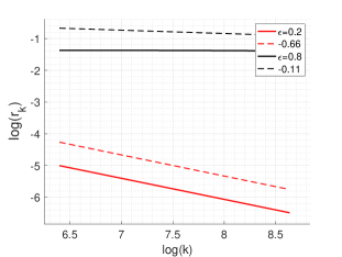
Figure 3: An example to verify equation (24) for $\epsilon\in\{0.2,0.8\}$. Solid and dashed lines denote the simulated dynamic in Lemma 3 and its corresponding theoretical rates, i.e., $\mathcal{O}(k^{-\frac{1-\epsilon}{1+\epsilon}})$, respectively. Numbers assigned to dashed lines indicate the slope of those lines.

∎

Appendix C Proofs for Section 4 and Additional Discussion

This Section is organized as follows. First, we elaborate on the intuition why one needs to resort to variance reduction techniques in order to improve over SGD analysis provided in Section 3. Then we highlight the key challenges associated with the analysis of variance reduced methods under global KŁ condition and introduce a new variance reduced method PAGER. We explain the intuition why PAGER overcomes the aforementioned challenges and improves over SGD in online case (1), and over SGD and GD in finite sum (2) case. Finally, we provide convergence guarantees for each setting in Theorems 4 and 5.

Why SGD is not enough?

Notice that the analysis in Section 3, in particular, implies that if we want to solve problem (1) using SGD with constant step-size $\eta$ and a mini-batch with replacement gradient estimator of size $b$, we immediately obtain a recursion

$$\delta_{t+1}-\delta_{t}\leq-\eta\mu\delta_{t}^{\frac{2}{\alpha}}+\frac{\eta^{2}L\sigma^{2}}{2b}.$$ (25)

It is easy to see that if $\eta$ is fixed, then the last (variance) term in the above recursion can be only controlled by selecting large enough $b$. Assume that we want to solve our problem to $\epsilon_{f}$ accuracy ($\delta_{T}\leq\epsilon_{f}$). Then to balance the two terms on the RHS, one needs to take $b\sim\epsilon_{f}^{-\frac{2}{\alpha}}$. This choice simplifies the recursion to $\delta_{t+1}-\delta_{t}\leq-\frac{\eta\mu}{2}\delta_{t}^{\frac{2}{\alpha}}$. Applying Lemma 6 with $c=\frac{2-\alpha}{\alpha}$, we conclude that one needs $T\sim\epsilon_{f}^{\frac{-(2-\alpha)}{\alpha}}$ iterations to reach $\delta_{T}\leq\epsilon_{f}$. Thus, the total sample complexity is $b\cdot T\sim\epsilon_{f}^{\frac{-(4-\alpha)}{\alpha}}$. This observation implies that we need to construct a more sophisticated gradient estimator than mini-batch estimator in order to improve the sample complexity of SGD.

Variance reduction and challenges under KŁ condition.

One common technique to design faster algorithms in stochastic optimization is to reduce variance of the gradient estimator using a control variate. It turns out that using such variance reduction techniques one can often design a gradient estimator at a much lower cost, while maintaining the same iteration complexity. Let us turn our attention to one popular variance reduction mechanism called PAGE. The main steps of PAGE method is described in Section 4, the detailed pseudo-code is presented in Algorithm 3. This method was originally proposed and analyzed for general non-convex and $2$-PŁ objectives [36]. However, its application to $\alpha$-PŁ functions with $\alpha\in[1,2)$ remains elusive. If we try to apply the standard analysis of PAGE, it will become apparent that we face several challenges. In particular, Lemma 8 along with Lemma 4 provides the following inequality for the iterates of the Algorithm 3

$$\Psi_{t+1}-\Psi_{t} \leq -\eta\mu\Psi_{t}^{\frac{2}{\alpha}}-\frac{p_{t}\lambda_{t}}{2}G_{t}\left(1-\frac{4\eta\mu}{p_{t}\alpha}\Psi_{t}^{\frac{2-\alpha}{\alpha}}\right)+\frac{p_{t}\lambda_{t}}{2}\frac{\sigma^{2}}{b_{t}},$$ (26)

where $\Psi_{t}=\delta_{t}+\lambda G_{t}$ is a candidate for a Lyapunov function and $G_{t}$ is the variance of the gradient estimator, and $\lambda>0$. To illustrate one key obstacle in the analysis of PAGE in online setting, let us set $G_{t}=0$ for simplicity

$$\Psi_{t+1}-\Psi_{t}\leq-\eta\mu\Psi_{t}^{\frac{2}{\alpha}}+\frac{p\lambda\sigma^{2}}{2b}.$$ (27)

Now, this recursion is very similar to (25). Therefore, the same argument applies here. In particular, one can argue that given constant parameters $\eta$, $b^{\prime}$ and $p$, we need to take $b\sim\epsilon_{f}^{-\frac{2}{\alpha}}$. Thus the total sample complexity is again no better than $b\cdot T\sim\epsilon_{f}^{\frac{-(4-\alpha)}{\alpha}}$. Note that the assumption $G_{t}=0$ was only made to illustrate one difficulty. Rigorously proving the fact that the term including $G_{t}$ is small constitutes another challenge.

Faster rates via PAGER in online case.

However, we notice that in (26), we have one more degree of freedom – the parameter $p$, which can be selected small enough to ensure smaller per iteration cost of the method. This intuition brings us to PAGER (Algorithm 2), a new modification of PAGE method with varying parameter $p$. We carefully select the sequences $\left\{p_{k}\right\}_{k\geq 0}$, $\left\{b_{k}\right\}_{k\geq 0}$, $\left\{b_{k}^{\prime}\right\}_{k\geq 0}$ for PAGER in order to obtain a small per iteration cost of order $p_{k}b_{k}+b_{k}^{\prime}\sim\epsilon_{f}^{-1}$. This leads to a much faster convergence with $\epsilon_{f}^{\nicefrac{{-2}}{{\alpha}}}$ sample complexity.

Difficulties in finite sum case and a fix via PAGER framework.

Let us now consider a finite sum problem (2) and directly apply Algorithm 3 with (constant) parameters $\eta$, $p$, $b$, $b^{\prime}$. Then we arrive at the following recursion

$$\Psi_{t+1}-\Psi_{t} \leq -\eta\mu\left(\Psi_{t}-\lambda G_{t}\right)^{\frac{2}{\alpha}}-\frac{p\lambda}{2}G_{t}$$

$$\leq -\eta\mu\Psi_{t}^{\frac{2}{\alpha}}-\frac{p\lambda}{2}G_{t}\left(1-\frac{4\eta\mu(n+1)}{\alpha}\Psi_{t}^{\frac{2-\alpha}{\alpha}}\right),$$

where we applied Lemma 8, 4 and selected optimal parameters $p=\frac{1}{n+1}$, $b=n$, $b^{\prime}=1$. By choosing a small enough stepsize $\eta$, we can unroll the above recursion and obtain the sample complexity ${\cal O}\big{(}\left(n\delta_{0}+\sqrt{n}\kappa\right)\left(\frac{1+\delta_{0}}{\epsilon_{f}}\right)^{\frac{2-\alpha}{\alpha}}\big{)}$, where $\delta_{0}=f(x_{0})-f^{\star}$, $\kappa=\nicefrac{{\mathcal{L}}}{{\mu}}$. However, this complexity is clearly not what one should hope for when analyzing a variance reduction scheme for problem (2). Notably, this complexity can be even worse than the one of standard GD, which is ${\cal O}\big{(}n\kappa\left(\frac{1+\delta_{0}}{\epsilon_{f}}\right)^{\frac{2-\alpha}{\alpha}}\big{)}$, for instance, when $\delta_{0}>\kappa$. The main reason for this slowdown is that in the analysis of Algorithm 3 with constant parameters, we are forced to take small step-sizes of order $\eta={\cal O}\big{(}\frac{1}{n\delta_{0}}\big{)}$ to ensure progress. Luckily, thanks to a flexible choice of parameters in PAGER, we can overcome this difficulty and provide improved convergence guaranties. Specifically, the framework of Algorithm 2 allows us to select an increasing sequence of step-sizes until it reaches the value $\eta={\cal O}\big{(}\frac{1}{\sqrt{n}\mathcal{L}}\big{)}$.

1:  Initialization: ${x}_{0},{g}_{0}\in\mathbb{R}^{d}$, step-size $\eta$ , number of iterations $T$, probability $p$, batch-sizes $b$, $b^{\prime}$

2:  for $t=0,\ldots,T-1$ do

3:     $x_{t+1}=x_{t}-\eta g_{t}$

4:     Sample $\chi\sim\text{Bernoulli}(p)$

5:     if $\chi=1$ then

6:        $g_{t+1}=\frac{1}{b}\sum_{i=1}^{b}\nabla f_{\xi_{t+1}^{i}}(x_{t+1})$

7:     else

8:        $g_{t+1}=g_{t}+\frac{1}{b^{\prime}}\sum_{i=1}^{b^{\prime}}\nabla f_{\xi_{t+1}^{i}}(x_{t+1})-\frac{1}{b^{\prime}}\sum_{i=1}^{b^{\prime}}\nabla f_{\xi_{t+1}^{i}}(x_{t})$

9:  Return: ${x}_{T}$

Algorithm 3 PAGE

C.1 Proof of Theorem 2

Now we state and prove a detailed version of Theorem 2.

Theorem 4.

Let $f(\cdot)$ have the form (1) and satisfy Assumptions 1, 3 (with $\alpha\in[1,2)$), 5 and 6, let the sequences in Algorithm 2 be chosen as

$$b_{k}^{\prime}=\frac{\alpha}{8\eta\mu}\left(\frac{2^{k}}{\bar{\Psi}_{0}}\right)^{\frac{2-\alpha}{\alpha}},\quad p_{k}=\frac{1}{1+b_{k}^{\prime}},$$

$$b_{k}=\left(\frac{2\cdot 2^{\frac{2-\alpha}{\alpha}}\cdot 2^{k}}{\bar{\Psi}_{0}}\right)^{\frac{2}{\alpha}}\frac{\sigma^{2}}{4\mu\eta^{2}\mathcal{L}^{2}},$$

$$T_{k}=\frac{2}{\eta\mu}\left(2\cdot 2^{\frac{2-\alpha}{\alpha}}\left(\frac{2^{k}U}{\bar{\Psi}_{0}}+2\left(\frac{\eta\mu}{2}\right)^{\frac{\alpha}{2-\alpha}}\right)\right)^{\frac{2-\alpha}{\alpha}},$$

$$\eta_{k}=\eta=\frac{1}{\mu}\min\left\{\frac{1}{2\kappa},\frac{\alpha}{8}\right\},$$

where $\bar{\Psi}_{0}:=f(\bar{x}_{0})-f(x^{\star})+\lambda_{0}\left\|\bar{g}_{0}-\nabla f(\bar{x}_{0})\right\|^{2}$, $\lambda_{0}:=\frac{b^{\prime}_{0}}{4\eta_{0}(1-p_{0})\mathcal{L}^{2}}$. Then, for any $\epsilon_{f}>0$ Algorithm 2 returns a point $\bar{x}_{K}$ with ${\mathbb{E}}\left[f(\bar{x}_{K})-f^{\star}\right]\leq\epsilon_{f}$ after $N:=\sum_{k=0}^{K-1}T_{k}={\cal O}\big{(}\epsilon_{f}^{-\frac{2-\alpha}{\alpha}}\big{)}$ iterations. The expected total computational cost (sample complexity) is

$$\text{cost}:=\sum_{k=0}^{K-1}T_{k}\left(p_{k}b_{k}+2(1-p_{k})b_{k}^{\prime}\right)={\cal O}\left(\epsilon_{f}^{-\frac{2}{\alpha}}\right).$$

Proof.

Combining the result of Lemma 8 and Lemma 4 with $a=\frac{2}{\alpha}$, $x=\frac{\lambda G_{t}}{\Psi_{t}}\leq 1$, we obtain the following recursion

$$\Psi_{t+1}-\Psi_{t} \leq -\eta\mu\Psi_{t}^{\frac{2}{\alpha}}-\frac{p_{k}\lambda_{k}}{2}G_{t}\left(1-\frac{4\eta\mu}{p_{k}\alpha}\Psi_{t}^{\frac{2-\alpha}{\alpha}}\right)+\frac{p_{k}\lambda_{k}}{2}\frac{\sigma^{2}}{b_{k}},$$ (28)

where ${\Psi}_{t}:=\delta_{t}+\lambda_{k}G_{t}$, $G_{t}:={\mathbb{E}}\left[\frac{1}{2}\left\|g_{t}-\nabla f(x_{t})\right\|^{2}\right]$, $\delta_{t}:={\mathbb{E}}\left[f(x_{t})-f(x^{\star})\right]$, $\lambda_{k}:=\frac{b^{\prime}_{k}}{4\eta_{k}(1-p_{k})\mathcal{L}^{2}}$.

Define the sequence $\left\{\bar{\Psi}_{k}\right\}_{k\geq 0}$ as $\bar{\Psi}_{k}:={\mathbb{E}}\left[f(\bar{x}_{k})-f(x^{\star})+\lambda_{k}\left\|\bar{g}_{k}-\nabla f(\bar{x}_{k})\right\|^{2}\right]$, which corresponds to the outer loop of the Algorithm 2. For each $k=0,\ldots,K-1$, the inner loop of Algorithm 2 starts with $x_{0}$ such that $\Psi_{0}:=\bar{\Psi}_{k}$. Let us prove by induction that within the outer loop $\bar{\Psi}_{k}\leq\frac{\bar{\Psi}_{0}}{2^{k}}$ for $k=0,\ldots,K-1$ and, for each $k=0,\ldots,K-1$, within the inner loop we have $\Psi_{t+1}\leq\Psi_{t}$ for $t=0,\ldots T_{k}-1$ (unless we reached the desired accuracy $\Psi_{t}\leq\frac{\bar{\Psi}_{k}}{2\cdot 2^{\frac{2-\alpha}{\alpha}}}$ within the inner loop). The induction base for the outer loop and $k=0$ is trivial. The induction base for the inner loop and $t=0$ is verified by the assumption on the step-size and the choice of batch-sizes when $k=0$. Fix $k=0,\ldots,K-1$ and $t=0,\ldots,T_{k}-1$ and assume that we have $\Psi_{t}\leq\Psi_{t-1}\leq\Psi_{0}=\bar{\Psi}_{k}$ and $\bar{\Psi}_{k}\leq\frac{\bar{\Psi}_{0}}{2^{k}}$. Then it follows from (28) that

$$\Psi_{t+1}-\Psi_{t} \leq -\eta\mu\Psi_{t}^{\frac{2}{\alpha}}-\frac{p_{k}\lambda_{k}}{2}G_{t}\left(1-\frac{4\eta\mu}{p_{k}\alpha}\Psi_{t}^{\frac{2-\alpha}{\alpha}}\right)+\frac{p_{k}\lambda_{k}}{2}\frac{\sigma^{2}}{b_{k}}$$

$$\leq -\eta\mu\Psi_{t}^{\frac{2}{\alpha}}-\frac{p_{k}\lambda_{k}}{2}G_{t}\left(1-\frac{4\eta\mu}{p_{k}\alpha}\bar{\Psi}_{k}^{\frac{2-\alpha}{\alpha}}\right)+\frac{p_{k}\lambda_{k}}{2}\frac{\sigma^{2}}{b_{k}}$$

$$\leq -\eta\mu\Psi_{t}^{\frac{2}{\alpha}}-\frac{p_{k}\lambda_{k}}{2}G_{t}\left(1-\frac{4\eta\mu}{p_{k}\alpha}\left(\frac{\bar{\Psi}_{0}}{2^{k}}\right)^{\frac{2-\alpha}{\alpha}}\right)+\frac{p_{k}\lambda_{k}}{2}\frac{\sigma^{2}}{b_{k}}$$

$$\overset{(i)}{\leq} -\eta\mu\Psi_{t}^{\frac{2}{\alpha}}+\frac{p_{k}\lambda_{k}}{2}\frac{\sigma^{2}}{b_{k}}$$

$$\overset{(ii)}{=} -\eta\mu\Psi_{t}^{\frac{2}{\alpha}}+\frac{p_{k}}{2}\frac{\sigma^{2}}{b_{k}}\frac{b_{k}^{\prime}}{4\eta(1-p_{k})\mathcal{L}^{2}}$$

$$\overset{(iii)}{=} -\eta\mu\Psi_{t}^{\frac{2}{\alpha}}+\frac{\sigma^{2}}{b_{k}}\frac{1}{8\eta\mathcal{L}^{2}}$$

$$\overset{(iv)}{=} -\eta\mu\Psi_{t}^{\frac{2}{\alpha}}+\frac{\eta\mu}{2}\left(\frac{\bar{\Psi}_{0}}{2\cdot 2^{\frac{2-\alpha}{\alpha}}\cdot 2^{k}}\right)^{\frac{2}{\alpha}}.$$

where $(i)$ follows by $p_{k}\geq\frac{1}{2b_{k}^{\prime}}=\frac{4\eta\mu}{\alpha}\left(\frac{\bar{\Psi}_{0}}{2^{k}}\right)^{\frac{2-\alpha}{\alpha}}$ and the assumption on the step-size, $(ii)$ is due to $\lambda_{k}=\frac{b_{k}^{\prime}}{4\eta(1-p_{k})\mathcal{L}^{2}}$, $(iii)$ is due to $\frac{p_{k}b_{k}^{\prime}}{1-p_{k}}=1$, and $(iv)$ holds by the assumption on the batch-size $b_{k}$. The above recursion guaranties that after at most $T_{k}=\frac{2}{\eta\mu}\left(2\cdot 2^{\frac{2-\alpha}{\alpha}}\left(\frac{2^{k}U}{\bar{\Psi}_{0}}+2\left(\frac{\eta\mu}{2}\right)^{\frac{\alpha}{2-\alpha}}\right)\right)^{\frac{2-\alpha}{\alpha}}$ inner loop iterations, we have $\Psi_{T_{k}}\leq\frac{\Psi_{0}}{4}=\frac{\bar{\Psi}_{k}}{2\cdot 2^{\frac{2-\alpha}{\alpha}}}=\frac{\bar{\Psi}_{0}}{2\cdot 2^{\frac{2-\alpha}{\alpha}}\cdot 2^{k}}$. Indeed, if for $t=0,\ldots,T_{k}-1$, we have not reached $\Psi_{t}\leq\frac{\bar{\Psi}_{0}}{2\cdot 2^{\frac{2-\alpha}{\alpha}}\cdot 2^{k}}$, then $\Psi_{t+1}-\Psi_{t}\leq-\frac{\eta\mu}{2}\Psi_{t}^{\frac{2}{\alpha}}\leq 0$ and by Lemma 6 (with $c=\frac{2-\alpha}{\alpha}$, $b=\nicefrac{{\eta\mu}}{{2}}$), we get $\Psi_{T_{k}}\leq\frac{\Psi_{0}}{2\cdot 2^{\frac{2-\alpha}{\alpha}}}=\frac{\bar{\Psi}_{k}}{2\cdot 2^{\frac{2-\alpha}{\alpha}}}$. Now it remains to analyze the outer loop of Algorithm 2. By the definition of $\bar{\Psi}_{k}$ and the choice of batch-sizes $b_{k}^{\prime}$ we have $\lambda_{k+1}\leq 2^{\frac{2-\alpha}{\alpha}}\lambda_{k}$ and $\bar{\Psi}_{{k+1}}\leq 2^{\frac{2-\alpha}{\alpha}}\Psi_{T_{k}}\leq\frac{\bar{\Psi}_{k}}{2}\leq\frac{\bar{\Psi}_{0}}{2^{k+1}}$. Thus, the induction step is complete.

In order to achieve $\bar{\Psi}_{K}\leq\epsilon_{f}$, we need $K=\log_{2}\left(\frac{\bar{\Psi}_{0}}{\epsilon_{f}}\right)$ outer loop iterations. The total number of iterations is

$$N = \sum_{k=0}^{K-1}T_{k}$$

$$= \sum_{k=0}^{K-1}\frac{2}{\eta\mu}\left(2\cdot 2^{\frac{2-\alpha}{\alpha}}\left(\frac{2^{k}U}{\bar{\Psi}_{0}}+2\left(\frac{\eta\mu}{2}\right)^{\frac{\alpha}{2-\alpha}}\right)\right)^{\frac{2-\alpha}{\alpha}}$$

$$= \frac{2}{\eta\mu}\left(2\cdot 2^{\frac{2-\alpha}{\alpha}}\right)^{\frac{2-\alpha}{\alpha}}\sum_{k=0}^{K-1}\left(\frac{2^{k}U}{\bar{\Psi}_{0}}+2\left(\frac{\eta\mu}{2}\right)^{\frac{\alpha}{2-\alpha}}\right)^{\frac{2-\alpha}{\alpha}}$$

$$= \frac{2\cdot 2^{\frac{2(2-\alpha)}{\alpha^{2}}}}{\eta\mu}\left(\frac{U}{\bar{\Psi}_{0}}+2\left(\frac{\eta\mu}{2}\right)^{\frac{\alpha}{2-\alpha}}\right)^{\frac{2-\alpha}{\alpha}}\sum_{k=0}^{K-1}\left(2^{\frac{2-\alpha}{\alpha}}\right)^{k}$$

$$\leq \frac{2\cdot 2^{\frac{2(2-\alpha)}{\alpha^{2}}}}{\eta\mu}\left(\frac{U}{\bar{\Psi}_{0}}+2\left(\frac{\eta\mu}{2}\right)^{\frac{\alpha}{2-\alpha}}\right)^{\frac{2-\alpha}{\alpha}}\left(2^{\frac{2-\alpha}{\alpha}}\right)^{K}\left(2^{\frac{2-\alpha}{\alpha}}-1\right)^{-1}$$

$$\leq \frac{2\cdot 2^{\frac{2(2-\alpha)}{\alpha^{2}}}}{\eta\mu}\left(\frac{U}{\bar{\Psi}_{0}}+2\left(\frac{\eta\mu}{2}\right)^{\frac{\alpha}{2-\alpha}}\right)^{\frac{2-\alpha}{\alpha}}\left(2^{\frac{2-\alpha}{\alpha}}-1\right)^{-1}\left(\frac{\bar{\Psi}_{0}}{\epsilon_{f}}\right)^{\frac{2-\alpha}{\alpha}}.$$

The expected computational cost per iteration is

$$p_{k}b_{k}+2(1-p_{k})b_{k}^{\prime} \leq \frac{b_{k}}{1+b_{k}^{\prime}}+2b_{k}^{\prime}$$

$$\leq \frac{b_{k}}{b_{k}^{\prime}}+2b_{k}^{\prime}$$

$$\leq \frac{\left(\frac{2\cdot 2^{\frac{2-\alpha}{\alpha}}\cdot 2^{k}}{\bar{\Psi}_{0}}\right)^{\frac{2}{\alpha}}\frac{\sigma^{2}}{4\mu\eta^{2}\mathcal{L}^{2}}}{\frac{\alpha}{8\eta\mu}\left(\frac{2^{k}}{\bar{\Psi}_{0}}\right)^{\frac{2-\alpha}{\alpha}}}+2\frac{\alpha}{8\eta\mu}\left(\frac{2^{k}}{\bar{\Psi}_{0}}\right)^{\frac{2-\alpha}{\alpha}}$$

$$\leq \left(2\cdot 2^{\frac{2-\alpha}{\alpha}}\right)^{\frac{2}{\alpha}}\frac{2\sigma^{2}}{\eta\mathcal{L}^{2}}\frac{2^{k}}{\bar{\Psi}_{0}}+\frac{\alpha}{4\eta\mu}\left(\frac{2^{k}}{\bar{\Psi}_{0}}\right)^{\frac{2-\alpha}{\alpha}}$$

$$\leq \frac{2\sigma^{2}\cdot 2^{\nicefrac{{4}}{{\alpha^{2}}}}}{4\eta\mathcal{L}^{2}}\frac{2^{k}}{\bar{\Psi}_{0}}+\frac{\alpha}{4\eta\mu}\left(\frac{2^{k}}{\bar{\Psi}_{0}}\right)^{\frac{2-\alpha}{\alpha}}$$

$$\leq \left(\frac{\sigma^{2}\cdot 2^{\nicefrac{{4}}{{\alpha^{2}}}}}{4\eta\mathcal{L}^{2}\bar{\Psi}_{0}}+\frac{\alpha}{4\eta\mu\bar{\Psi}_{0}^{\frac{2-\alpha}{\alpha}}}\right){2^{k}}.$$

Denote $A:=\left(\frac{\sigma^{2}\cdot 2^{\nicefrac{{4}}{{\alpha^{2}}}}}{4\eta\mathcal{L}^{2}\bar{\Psi}_{0}}+\frac{\alpha}{4\eta\mu\bar{\Psi}_{0}^{\frac{2-\alpha}{\alpha}}}\right)$, then the total cost is

cost $$= \sum_{k=0}^{K-1}T_{k}\left(p_{k}b_{k}+2(1-p_{k})b_{k}^{\prime}\right)$$

$$= A\sum_{k=0}^{K-1}T_{k}\cdot{2^{k}}$$

$$= A\sum_{k=0}^{K-1}\frac{2}{\eta\mu}\left(2\cdot 2^{\frac{2-\alpha}{\alpha}}\left(\frac{2^{k}U}{\bar{\Psi}_{0}}+2\left(\frac{\eta\mu}{2}\right)^{\frac{\alpha}{2-\alpha}}\right)\right)^{\frac{2-\alpha}{\alpha}}2^{k}$$

$$= {2\cdot 2^{\frac{2(2-\alpha)}{\alpha^{2}}}A}\left(\frac{2}{\eta\mu}\left(\frac{U}{\bar{\Psi}_{0}}\right)^{\frac{2-\alpha}{\alpha}}\sum_{k=0}^{K-1}\left(2^{k}\right)^{\frac{2-\alpha}{\alpha}}2^{k}+2^{\frac{2-\alpha}{\alpha}}\sum_{k=0}^{K-1}2^{k}\right)$$

$$= {2\cdot 2^{\frac{2(2-\alpha)}{\alpha^{2}}}A}\left(\frac{2}{\eta\mu}\left(\frac{U}{\bar{\Psi}_{0}}\right)^{\frac{2-\alpha}{\alpha}}\sum_{k=0}^{K-1}\left(2^{k}\right)^{\frac{2}{\alpha}}+2^{\frac{2-\alpha}{\alpha}}\sum_{k=0}^{K-1}2^{k}\right)$$

$$= {2\cdot 2^{\frac{2(2-\alpha)}{\alpha^{2}}}A}\left(\frac{2}{\eta\mu}\left(\frac{U}{\bar{\Psi}_{0}}\right)^{\frac{2-\alpha}{\alpha}}\left(2^{K}\right)^{\frac{2}{\alpha}}\left(2^{\nicefrac{{2}}{{\alpha}}}-1\right)^{-1}+2^{\frac{2-\alpha}{\alpha}}2^{K}\right),$$

which further simplifies by using the value of $A$ and the step-size

cost $$= {\cal O}\left(\frac{A}{\eta\mu}\left(\frac{1}{\bar{\Psi}_{0}}\right)^{\frac{2-\alpha}{\alpha}}\left(2^{K}\right)^{\frac{2}{\alpha}}\right)$$

$$= {\cal O}\left(\frac{A}{\eta\mu}\left(\frac{1}{\bar{\Psi}_{0}}\right)^{\frac{2-\alpha}{\alpha}}\left(\frac{\bar{\Psi}_{0}}{\epsilon_{f}}\right)^{\frac{2}{\alpha}}\right)$$

$$= {\cal O}\left(\frac{A\bar{\Psi}_{0}}{\eta\mu}\left(\frac{1}{\epsilon_{f}}\right)^{\frac{2}{\alpha}}\right)$$

$$= {\cal O}\left(\left(\frac{\sigma^{2}}{\mu}+\frac{\bar{\Psi}_{0}^{\frac{2(\alpha-1)}{\alpha}}}{\eta^{2}\mu^{2}}\right)\left(\frac{1}{\epsilon_{f}}\right)^{\frac{2}{\alpha}}\right)$$

$$= {\cal O}\left(\left(\frac{\sigma^{2}}{\mu}+\kappa^{2}\bar{\Psi}_{0}^{\frac{2(\alpha-1)}{\alpha}}\right)\left(\frac{1}{\epsilon_{f}}\right)^{\frac{2}{\alpha}}\right)$$

$$= {\cal O}\left(\epsilon_{f}^{\nicefrac{{-2}}{{\alpha}}}\right).$$

∎

C.2 Proof of Theorem 3

Now we state and prove a detailed version of Theorem 3.

Theorem 5.

Let $f(\cdot)$ have the form (2) and satisfy Assumptions 1, 3 (with $\alpha\in[1,2)$) and 6, let the sequences in Algorithm 2 be chosen as $p_{k}=\frac{1}{n+1}$, $b_{k}^{\prime}=1$, $b_{k}=n$,

$$T_{k}=\frac{1}{\eta_{k}\mu}\left(\frac{U2^{k+1}}{\bar{\Psi}_{0}}+2\left(\eta_{k}\mu\right)^{\frac{\alpha}{2-\alpha}}\right)^{\frac{2-\alpha}{\alpha}},$$

$$\eta_{k}=\min\left\{\frac{1}{2\sqrt{n}\mathcal{L}},\frac{\alpha}{4\mu(n+1)}\left(\frac{2^{k}}{\bar{\Psi}_{0}}\right)^{\frac{2-\alpha}{\alpha}}\right\},$$

where $\bar{\Psi}_{0}:=f(\bar{x}_{0})-f(x^{\star})+\lambda_{0}\left\|\bar{g}_{0}-\nabla f(\bar{x}_{0})\right\|^{2}$, $\lambda_{0}:=\frac{b^{\prime}}{4\eta_{0}(1-p)\mathcal{L}^{2}}$ Then, for any $\epsilon_{f}>0$, Algorithm 2 returns a point $\bar{x}_{K}$ with ${\mathbb{E}}\left[f(\bar{x}_{K})-f^{\star}\right]\leq\epsilon_{f}$ after

$$N := \sum_{k=0}^{K-1}T_{k}={\cal\widetilde{O}}\left(n+\sqrt{n}\kappa\epsilon_{f}^{-\frac{2-\alpha}{\alpha}}\right)$$

iterations. The expected total computational cost (sample complexity) is

$$\text{cost}:=\sum_{k=0}^{K-1}T_{k}\left(p_{k}b_{k}+2(1-p_{k})b_{k}^{\prime}\right)={\cal\widetilde{O}}\left(n+\sqrt{n}\kappa\epsilon_{f}^{-\frac{2-\alpha}{\alpha}}\right).$$

Proof.

Combining the result of Lemma 8 and Lemma 4 with $a=\frac{2}{\alpha}$, $x=\frac{\lambda G_{t}}{\Psi_{t}}\leq 1$ and noticing that $\sigma^{2}=0$, we obtain the following recursion

$$\Psi_{t+1}-\Psi_{t} \leq -\eta\mu\Psi_{t}^{\frac{2}{\alpha}}-\frac{p\lambda}{2}G_{t}\left(1-\frac{4\eta\mu(n+1)}{\alpha}\Psi_{t}^{\frac{2-\alpha}{\alpha}}\right),$$ (29)

where ${\Psi}_{t}:=\delta_{t}+\lambda_{k}G_{t}$, $G_{t}:={\mathbb{E}}\left[\frac{1}{2}\left\|g_{t}-\nabla f(x_{t})\right\|^{2}\right]$, $\delta_{t}:={\mathbb{E}}\left[f(x_{t})-f(x^{\star})\right]$, $\lambda_{k}:=\frac{b^{\prime}}{4\eta_{k}(1-p)\mathcal{L}^{2}}$.

Define the sequence $\left\{\bar{\Psi}_{k}\right\}_{k\geq 0}$ as $\bar{\Psi}_{k}:={\mathbb{E}}\left[f(\bar{x}_{k})-f(x^{\star})+\lambda_{k}\left\|\bar{g}_{k}-\nabla f(\bar{x}_{k})\right\|^{2}\right]$ and $\lambda_{k}:=\frac{b^{\prime}}{4\eta_{k}(1-p)\mathcal{L}^{2}}$, which corresponds to the outer loop of the algorithm. For each $k=0,\ldots,K-1$, the inner loop of Algorithm 2 starts with $x_{0}$ such that $\Psi_{0}:=\bar{\Psi}_{k}$. Let us prove by induction that the sequence $\left\{\bar{\Psi}_{k}\right\}_{k\geq 0}$ satisfies $\bar{\Psi}_{k}\leq\frac{\bar{\Psi}_{0}}{2^{k}}$ for all $k=0,\ldots,K-1$. The induction base for $k=0$ is trivial. Let us prove the induction step for $k+1$. The evolution of the inner loop is characterized by (34) and given the assumption on the step-size, we have $\Psi_{t+1}-\Psi_{t}\leq-\eta\mu\Psi_{t}^{\frac{2}{\alpha}}$ for all $t=0,\ldots,T_{k}-1$ . Therefore, by Lemma 6 (with $c=\frac{2-\alpha}{\alpha}$, $b=\eta\mu$) we have

$$\Psi_{T_{k}} \leq\frac{U+\left(\eta_{k}\mu\right)^{\frac{\alpha}{2-\alpha}}\bar{\Psi}_{k}}{\left(\eta_{k}\mu T_{k}\right)^{\frac{\alpha}{2-\alpha}}}=\frac{U+\left(\eta_{k}\mu\right)^{\frac{\alpha}{2-\alpha}}\bar{\Psi}_{k}}{\frac{U\cdot 2^{k+1}}{\bar{\Psi}_{0}}+2\left(\eta_{k}\mu\right)^{\frac{\alpha}{2-\alpha}}}$$

$$=\frac{U+\left(\eta_{k}\mu\right)^{\frac{\alpha}{2-\alpha}}\bar{\Psi}_{k}}{U+\left(\eta_{k}\mu\right)^{\frac{\alpha}{2-\alpha}}\frac{\bar{\Psi}_{0}}{2^{k}}}\cdot\frac{\bar{\Psi}_{0}}{2^{k+1}}\overset{(i)}{\leq}\frac{\bar{\Psi}_{0}}{2^{k+1}},$$

where in $(i)$, we used $\bar{\Psi}_{k}\leq\frac{\bar{\Psi}_{0}}{2^{k}}$. Furthermore, since $\eta_{k+1}\geq\eta_{k}$, then $\lambda_{k+1}\leq\lambda_{k}$ and $\bar{\Psi}_{{k+1}}\leq\Psi_{T_{k}}\leq\frac{\bar{\Psi}_{0}}{2^{k+1}}$, and the induction step is complete.

In order to achieve $\bar{\Psi}_{K}\leq\epsilon_{f}$, we need $K=\log_{2}\left(\frac{\bar{\Psi}_{0}}{\epsilon_{f}}\right)$ outer loop iterations. The total number of iterations is

$$N = \sum_{k=0}^{K-1}T_{k}$$

$$\overset{(i)}{\leq} \sum_{k=0}^{K-1}\max\left\{\frac{4(n+1)}{\alpha}\left(\frac{\bar{\Psi}_{0}}{2^{k}}\right)^{\frac{(2-\alpha)}{\alpha}},2\sqrt{n}\kappa\right\}\left(\frac{U2^{k+1}}{\bar{\Psi}_{0}}+\frac{\mu}{\sqrt{n}\mathcal{L}}\right)^{\frac{2-\alpha}{\alpha}}$$

$$\leq \sum_{k=0}^{K-1}\max\left\{\frac{4(n+1)}{\alpha}\left(2\left(U+\frac{\bar{\Psi}_{0}}{\sqrt{n}\kappa}\right)\right)^{\frac{2-\alpha}{\alpha}},2\sqrt{n}\kappa\left(\frac{2U}{\bar{\Psi}_{0}}+\frac{1}{\sqrt{n}\kappa}\right)^{\frac{2-\alpha}{\alpha}}\left(2^{\frac{2-\alpha}{\alpha}}\right)^{k}\right\}$$

$$\leq \max\left\{\frac{4(n+1)}{\alpha}\left(2\left(U+\frac{\bar{\Psi}_{0}}{\sqrt{n}\kappa}\right)\right)^{\frac{2-\alpha}{\alpha}}K,2\sqrt{n}\kappa\left(\frac{2U}{\bar{\Psi}_{0}}+\frac{1}{\sqrt{n}\kappa}\right)^{\frac{2-\alpha}{\alpha}}\left(2^{\frac{2-\alpha}{\alpha}}\right)^{K}\left(2^{\frac{2-\alpha}{\alpha}}-1\right)^{-1}\right\}$$

$$\leq \max\left\{\frac{4(n+1)}{\alpha}\left(2\left(U+\frac{\bar{\Psi}_{0}}{\sqrt{n}\kappa}\right)\right)^{\frac{2-\alpha}{\alpha}}\log_{2}\left(\frac{\bar{\Psi}_{0}}{\epsilon_{f}}\right),\frac{2\sqrt{n}}{2^{\frac{2-\alpha}{\alpha}}-1}\kappa\left(\frac{2U}{\bar{\Psi}_{0}}+\frac{1}{\sqrt{n}\kappa}\right)^{\frac{2-\alpha}{\alpha}}\left(\frac{\bar{\Psi}_{0}}{\epsilon_{f}}\right)^{\frac{2-\alpha}{\alpha}}\right\}$$

$$= {\cal\widetilde{O}}\left(n+\sqrt{n}\kappa\epsilon_{f}^{-\frac{2-\alpha}{\alpha}}\right),$$

where in $(i)$ we used the assumption on the step-sizes. The expected computational cost per iteration is ${p_{k}b_{k}+2(1-p_{k})b_{k}^{\prime}}\leq 3$ and thus the total cost is ${\cal\widetilde{O}}\big{(}n+\sqrt{n}\kappa\epsilon_{f}^{-\frac{2-\alpha}{\alpha}}\big{)}$. ∎

C.3 Technical lemmas

Lemma 4.

Let $x\leq 1$ and $a\geq 1$, then $(1-x)^{a}\geq 1-ax$.

Proof.

The results follows directly by applying the definition of convexity. ∎

The following lemma is standard, we provide its proof for completeness.

Lemma 5.

Suppose that function $f(\cdot)$ is $L$-smooth and let $x_{t+1}:=x_{t}-\eta g_{t},$ where $g_{t}\in\mathbb{R}^{d}$ is any vector, and $\eta>0$ any scalar. Then we have

$$f(x_{t+1})\leq f(x_{t})-\frac{\eta}{2}\left\|\nabla f(x_{t})\right\|^{2}-\left(\frac{1}{2\eta}-\frac{L}{2}\right)\left\|x_{t+1}-x_{t}\right\|^{2}+\frac{\eta}{2}\left\|g_{t}-\nabla f(x_{t})\right\|^{2}.$$ (30)

Proof.

Define $\bar{x}_{t+1}:=x_{t}-\eta\nabla f\left(x_{t}\right)$, then using Assumption 1 after some rearrangements we obtain

$$f\left(x_{t+1}\right) {\leq} f\left(x_{t}\right)+\left\langle\nabla f\left(x_{t}\right),x_{t+1}-x_{t}\right\rangle+\frac{L}{2}\left\|x_{t+1}-x_{t}\right\|^{2}$$

$$= f\left(x_{t}\right)+\left\langle\nabla f\left(x_{t}\right)-g_{t},x_{t+1}-x_{t}\right\rangle+\left\langle g_{t},x_{t+1}-x_{t}\right\rangle+\frac{L}{2}\left\|x_{t+1}-x_{t}\right\|^{2}$$

$$= f\left(x_{t}\right)+\left\langle\nabla f\left(x_{t}\right)-g_{t},-\eta g_{t}\right\rangle-\left(\frac{1}{\eta}-\frac{L}{2}\right)\left\|x_{t+1}-x_{t}\right\|^{2}$$

$$= f\left(x_{t}\right)+\eta\left\|\nabla f\left(x_{t}\right)-g_{t}\right\|^{2}-\eta\left\langle\nabla f\left(x_{t}\right)-g_{t},\nabla f\left(x_{t}\right)\right\rangle-\left(\frac{1}{\eta}-\frac{L}{2}\right)\left\|x_{t+1}-x_{t}\right\|^{2}$$

$$= f\left(x_{t}\right)+\eta\left\|\nabla f\left(x_{t}\right)-g_{t}\right\|^{2}-\frac{1}{\eta}\left\langle x_{t+1}-\bar{x}_{t+1},x_{t}-\bar{x}_{t+1}\right\rangle-\left(\frac{1}{\eta}-\frac{L}{2}\right)\left\|x_{t+1}-x_{t}\right\|^{2}$$

$$= f\left(x_{t}\right)+\eta\left\|\nabla f\left(x_{t}\right)-g_{t}\right\|^{2}-\left(\frac{1}{\eta}-\frac{L}{2}\right)\left\|x_{t+1}-x_{t}\right\|^{2}$$

$$\qquad-\frac{1}{2\eta}\left(\left\|x_{t+1}-\bar{x}_{t+1}\right\|^{2}+\left\|x_{t}-\bar{x}_{t+1}\right\|^{2}-\left\|x_{t+1}-x_{t}\right\|^{2}\right)$$

$$= f\left(x_{t}\right)+\eta\left\|\nabla f\left(x_{t}\right)-g_{t}\right\|^{2}-\left(\frac{1}{\eta}-\frac{L}{2}\right)\left\|x_{t+1}-x_{t}\right\|^{2}$$

$$\qquad-\frac{1}{2\eta}\left(\eta^{2}\left\|\nabla f\left(x_{t}\right)-g_{t}\right\|^{2}+\eta^{2}\left\|\nabla f\left(x_{t}\right)\right\|^{2}-\left\|x_{t+1}-x_{t}\right\|^{2}\right)$$

$$= f\left(x_{t}\right)-\frac{\eta}{2}\left\|\nabla f\left(x_{t}\right)\right\|^{2}-\left(\frac{1}{2\eta}-\frac{L}{2}\right)\left\|x_{t+1}-x_{t}\right\|^{2}+\frac{\eta}{2}\left\|g_{t}-\nabla f\left(x_{t}\right)\right\|^{2}.$$

∎

Lemma 6.

Let $\left\{r_{k}\right\}_{k\geq 0}$ be a non-negative sequence, which satisfies

$$r_{k+1}\leq r_{k}(1-br_{k}^{c}),\quad\text{for all }k$$

and $c>0$. Then

$$r_{k}\leq\frac{U+b^{\nicefrac{{1}}{{c}}}r_{0}}{\left(b\left(k+1\right)\right)^{\nicefrac{{1}}{{c}}}},$$

where $U:=2^{\nicefrac{{1}}{{c}}}\cdot c^{-\frac{2}{c}-1}+c^{-\nicefrac{{1}}{{c}}}$.

Proof.

Define $u_{k}:=\varphi(k)r_{k}$, $\varphi(k):=\left(b(k+1)\right)^{\nicefrac{{1}}{{c}}}$. Then using $\varphi(k+1)-\varphi(k)\leq\frac{1}{c}\frac{\varphi(k+1)}{k+2}$ and $1\leq\varphi(k+1)\left(\varphi(k)\right)^{-1}\leq 2^{\nicefrac{{1}}{{c}}}$, we obtain

$$u_{k+1}-u_{k} = \varphi(k+1)r_{k+1}-\varphi(k)r_{k}$$

$$\leq \left(\varphi(k+1)-\varphi(k)\right)r_{k}-b\varphi(k+1)r_{k}^{1+c}$$

$$= \left(\varphi(k+1)-\varphi(k)\right)\left(\varphi(k)\right)^{-1}u_{k}-b\varphi(k+1)\left(\varphi(k)\right)^{-1-c}u_{k}^{1+c}$$

$$= \left(\varphi(k+1)-\varphi(k)\right)\left(\varphi(k)\right)^{-1}u_{k}\left(1-\frac{\varphi(k+1)u_{k}^{c}}{(k+1)\left(\varphi(k+1)-\varphi(k)\right)}\right)$$

$$\leq \left(\varphi(k+1)-\varphi(k)\right)\left(\varphi(k)\right)^{-1}u_{k}\left(1-cu_{k}^{c}\right).$$

It follows from the above recursion that the sequence $\left\{u_{k}\right\}_{k\geq 0}$ is bounded for all $k$. Indeed, define $F(k,u):=\left(\varphi(k+1)-\varphi(k)\right)\left(\varphi(k)\right)^{-1}u\left(1-cu^{c}\right)$. Notice that for all $k\geq 0$ and $u>c^{-\nicefrac{{1}}{{c}}}$ we have $F(k,u)<0$ and for all $k,u\geq 0$ we have $F(k,u)\leq 2^{\nicefrac{{1}}{{c}}}\cdot c^{-\frac{2}{c}-1}$. Now it is straightforward to see that $u_{k}\leq u_{0}+2^{\nicefrac{{1}}{{c}}}\cdot c^{-\frac{2}{c}-1}+c^{-\nicefrac{{1}}{{c}}}$. It only remains to return to $r_{k}$ sequence to obtain the desired result. ∎

Lemma 7 (Lemma 4 of [36]).

Let Assumptions 5 and 6 hold, and let for $\chi\sim\text{Bernoulli}(p)$ and $g_{t}\in\mathbb{R}^{d}$, we construct $g_{t+1}$ via

$$g_{t+1}=\begin{cases}\frac{1}{b}\sum_{i=1}^{b}\nabla f_{\xi_{t+1}^{i}}(x_{t+1})&\text{if}\quad\ \chi=1,\\ g_{t}+\frac{1}{b^{\prime}}\sum_{i=1}^{b^{\prime}}\left(\nabla f_{\xi_{t+1}^{i}}(x_{t+1})-\nabla f_{\xi_{t+1}^{i}}(x_{t})\right)&\text{if}\quad\ \chi=0.\end{cases}$$ (31)

Then

$$G_{t+1}-G_{t}\leq-p{G_{t}}+\frac{(1-p)\mathcal{L}^{2}}{b^{\prime}}R_{t}+\frac{p\sigma^{2}}{2b},$$ (32)

where $G_{t}:={\mathbb{E}}\left[\frac{1}{2}\left\|g_{t}-\nabla f(x_{t})\right\|^{2}\right]$, $R_{n}:={\mathbb{E}}\left[\frac{1}{2}\left\|x_{t+1}-x_{t}\right\|^{2}\right]$.

Proof.

$$G_{t+1} = \mathbb{E}\left[\frac{1}{2}\left\|g_{t+1}-\nabla f\left(x_{t+1}\right)\right\|^{2}\right]$$

$$= p\mathbb{E}\left[\frac{1}{2}\left\|\frac{1}{b}\sum_{i=1}^{b}\nabla f_{\xi_{t+1}^{i}}(x_{t+1})-\nabla f\left(x_{t+1}\right)\right\|^{2}\right]$$

$$\qquad+\left(1-p\right){\mathbb{E}}\left[\frac{1}{2}\left\|g_{t}+\frac{1}{b^{\prime}}\sum_{i=1}^{b^{\prime}}\left(\nabla f_{\xi_{t+1}^{i}}(x_{t+1})-\nabla f_{\xi_{t+1}^{i}}(x_{t})\right)-\nabla f\left(x_{t+1}\right)\right\|^{2}\right]$$

$$\leq \frac{p\sigma^{2}}{2b}+\left(1-p\right){\mathbb{E}}\left[\frac{1}{2}\left\|g_{t}+\frac{1}{b^{\prime}}\sum_{i=1}^{b^{\prime}}\left(\nabla f_{\xi_{t+1}^{i}}(x_{t+1})-\nabla f_{\xi_{t+1}^{i}}(x_{t})\right)-\nabla f\left(x_{t+1}\right)\right\|^{2}\right]$$

$$= \ \frac{p\sigma^{2}}{2b}+\left(1-p\right){\mathbb{E}}\left[\frac{1}{2}\left\|g_{t}-\nabla f\left(x_{t}\right)+\widetilde{\Delta}(x_{t+1},x_{t})-\Delta(x_{t+1},x_{t})\right\|^{2}\right]$$

$$= \frac{p\sigma^{2}}{2b}+\left(1-p\right){\mathbb{E}}\left[\frac{1}{2}\left\|g_{t}-\nabla f\left(x_{t}\right)\right\|^{2}\right]+\left(1-p\right){\mathbb{E}}\left[\frac{1}{2}\left\|\widetilde{\Delta}(x_{t+1},x_{t})-\Delta(x_{t+1},x_{t})\right\|^{2}\right]$$

$$\leq \left(1-p\right){\mathbb{E}}\left[\frac{1}{2}\left\|g_{t}-\nabla f\left(x_{t}\right)\right\|^{2}\right]+\frac{(1-p)\mathcal{L}^{2}}{b^{\prime}}{\mathbb{E}}\left[\frac{1}{2}\left\|x_{t+1}-x_{t}\right\|^{2}\right]+\frac{p\sigma^{2}}{2b}$$

$$= \left(1-p\right)G_{t}+\frac{(1-p)\mathcal{L}^{2}}{b^{\prime}}R_{t}+\frac{p\sigma^{2}}{2b},$$

where the first inequality holds by Assumption 5 and the second inequality is due to Assumption 6 with $\widetilde{\Delta}(x,y):=\frac{1}{b^{\prime}}\sum_{i=1}^{b^{\prime}}\left(\nabla f_{\xi_{t+1}^{i}}(x)-\nabla f_{\xi_{t+1}^{i}}(y)\right)$, $\Delta(x,y):=\nabla f(x)-\nabla f(y)$, $x=x_{t+1}$, $y=x_{t}$.

∎

Lemma 8.

Let $f(\cdot)$ satisfy Assumptions 1, 3, 5 and 6. Assume that the step-size in Algorithm 3 satisfies

$$\eta\leq\min\left\{\frac{1}{2L},\sqrt{\frac{pb^{\prime}}{1-p}}\frac{1}{2\mathcal{L}}\right\}.$$ (33)

Define $\Psi_{t}:={\mathbb{E}}\left[f(x_{t})-f(x^{\star})+\lambda\left\|g_{t}-\nabla f(x_{t})\right\|^{2}\right]$, $\lambda:=\frac{b^{\prime}}{4\eta(1-p)\mathcal{L}^{2}}$. Then Algorithm 3 generates a sequence of points $\left\{x_{t}\right\}_{t\geq 0}$ such that

$$\Psi_{t+1}-\Psi_{t} \leq -\eta\mu\left(\Psi_{t}-\lambda G_{t}\right)^{\frac{2}{\alpha}}-\frac{p\lambda}{2}G_{t}+\frac{p\lambda}{2}\frac{\sigma^{2}}{b}.$$ (34)

Proof.

Using the notation $G_{t}:={\mathbb{E}}\left[\frac{1}{2}\left\|g_{t}-\nabla f(x_{t})\right\|^{2}\right]$, $R_{t}:={\mathbb{E}}\left[\frac{1}{2}\left\|x_{t+1}-x_{t}\right\|^{2}\right]$, $\delta_{t}:={\mathbb{E}}\left[f(x_{t})-f(x^{\star})\right]$ and assumption on the step-size $\eta\leq\frac{1}{2L}$, it follows by Lemma 5 that

$$\delta_{t+1}-\delta_{t}\leq-\frac{\eta}{2}{\mathbb{E}}\left[\left\|\nabla f(x_{t})\right\|^{2}\right]-\frac{1}{2\eta}R_{t}+{\eta}G_{t}.$$

Using Assumption 3, Jensen’s inequality for $x\mapsto x^{\frac{2}{\alpha}}$, we get

$$\delta_{t+1}-\delta_{t}\leq-\eta\mu\delta_{t}^{\frac{2}{\alpha}}+{\eta}G_{t}-\frac{1}{2\eta}R_{t}.$$

For $p<1$, it follows from Lemma 7 that

$$-R_{t}\leq-\frac{b^{\prime}}{(1-p)\mathcal{L}^{2}}\left(G_{t+1}-G_{t}\right)-\frac{pb^{\prime}}{(1-p)\mathcal{L}^{2}}{G_{t}}+\frac{b^{\prime}}{(1-p)\mathcal{L}^{2}}\frac{p\sigma^{2}}{2b}.$$

Thus, combining the above two inequalities, we get

$$\delta_{t+1}-\delta_{t}+\frac{1}{2\eta}\frac{b^{\prime}}{(1-p)\mathcal{L}^{2}}\left(G_{t+1}-G_{t}\right)\leq-\eta\mu\delta_{t}^{\frac{2}{\alpha}}-\left(\frac{1}{2\eta}\frac{pb^{\prime}}{(1-p)\mathcal{L}^{2}}-\eta\right)G_{t}+\frac{1}{2\eta}\frac{b^{\prime}}{(1-p)\mathcal{L}^{2}}\frac{p\sigma^{2}}{2b}.$$

Let $\Psi_{t}:=\delta_{t}+\lambda G_{t}$, $\lambda:=\frac{b^{\prime}}{2\eta(1-p)\mathcal{L}^{2}}$. Using the assumption on the step-size, $\eta\leq\sqrt{\frac{pb^{\prime}}{4(1-p)\mathcal{L}^{2}}}$, we get

$$\Psi_{t+1}-\Psi_{t} = \delta_{t+1}-\delta_{t}+\lambda\left(G_{t+1}-G_{t}\right)$$

$$= \delta_{t+1}-\delta_{t}+\frac{b^{\prime}}{2\eta(1-p)\mathcal{L}^{2}}\left(G_{t+1}-G_{t}\right)$$

$$\leq -\eta\mu\delta_{t}^{\frac{2}{\alpha}}-\frac{pb^{\prime}}{4\eta(1-p)\mathcal{L}^{2}}G_{t}+\frac{1}{2\eta}\frac{b^{\prime}}{(1-p)\mathcal{L}^{2}}\frac{p\sigma^{2}}{2b}$$

$$= -\eta\mu\delta_{t}^{\frac{2}{\alpha}}-\frac{p\lambda}{2}G_{t}+\frac{p\lambda}{2}\frac{\sigma^{2}}{b}$$

$$= -\eta\mu\left(\Psi_{t}-\lambda G_{t}\right)^{\frac{2}{\alpha}}-\frac{p\lambda}{2}G_{t}+\frac{p\lambda}{2}\frac{\sigma^{2}}{b}.$$

∎

Appendix D Convergence in the Iterates

In this Section, we assume that $\alpha$-PŁ condition holds with $\alpha\in(1,2]$. We provide convergence guaranties in the iterates to the set of optimal points $X^{\star}$, which we assume to be non-empty. The sample complexity results are summarized in Table 2. The results in Table 2 are obtained by translating the sample complexity results reported in Table 1 to convergence in the iterates via Proposition 4. Note that in the special case $\alpha=2$, our rates in both Tables 1 and 2 recover the optimal rates for online case [26, 23, 30] and the best known results for finite sum case [49, 36].

Proposition 4.

Let Assumption 3 hold with $\alpha\in(1,2]$ and the set of optimal points $X^{\star}:=\operatorname*{arg\,min}_{x}f(x)$ is not empty. Then

$$dist\left(x,X^{\star}\right)\leq\frac{\alpha}{\alpha-1}\frac{1}{\sqrt{2\mu}}\left(f(x)-f^{\star}\right)^{\frac{\alpha-1}{\alpha}}\quad\text{for all }x\in\mathbb{R}^{d},$$ (35)

where $dist\left(x,X^{\star}\right):=\min_{y\in X^{\star}}\left\|y-x\right\|$.

The above result can be obtained by following the argument similar to the proof of Theorem 2 in [26] (where it is shown for a particular case $\alpha=2$). The only difference is that one should take a disingularizing function as $g(x)=\left(f(x)-f^{\star}\right)^{\frac{\alpha-1}{\alpha}}$, where $f^{\star}=\min_{x}f(x)$. This result immediately implies convergence in the iterates via

$${\mathbb{E}}\left[\min_{y\in X^{\star}}\left\|x-y\right\|\right] = {\mathbb{E}}\left[dist\left(x,X^{\star}\right)\right]$$ (36)

$$\overset{\eqref{eq:f_to_x}}{\leq} \frac{\alpha}{\alpha-1}\frac{1}{\sqrt{2\mu}}{\mathbb{E}}\left[\left(f(x)-f^{\star}\right)^{\frac{\alpha-1}{\alpha}}\right]$$

$$\leq \frac{\alpha}{\alpha-1}\frac{1}{\sqrt{2\mu}}\left({\mathbb{E}}\left[f(x)-f^{\star}\right]\right)^{\frac{\alpha-1}{\alpha}},$$

where the last inequality holds by Jensen’s inequality for a concave function $t\mapsto t^{\frac{\alpha-1}{\alpha}}$.

Table 2: Summary of sample complexity results for $\alpha$-PŁ functions (Assumption 3) with $\alpha\in(1,2]$ under average $\mathcal{L}$-smoothness (Assumptions 6) and bounded variance (Assumptions 5). Quantities: $\alpha$ = PL power; $\mu$ = PL constant; $\kappa=\nicefrac{{\mathcal{L}}}{{\mu}}$; $\sigma^{2}$ = variance. The entries of the table show the expected number of stochastic gradient calls to achieve ${\mathbb{E}}\left[dist\left(x,X^{\star}\right)\right]\leq\epsilon_{x}$, where $X^{\star}\neq\emptyset$ is the set of optimal points of $f(\cdot)$.

Method	Finite sum case	Online case
GD	${\cal O}\left({n\kappa}{\mu^{\frac{\alpha-2}{2(\alpha-1)}}}\left(\frac{1}{\epsilon_{x}}\right)^{\frac{2-\alpha}{\alpha-1}}\right)$	N/A
SGD	${\cal O}\left(\kappa\sigma^{2}\mu^{\frac{\alpha+2}{2(1-\alpha)}}\left(\frac{1}{\epsilon_{x}}\right)^{\frac{4-\alpha}{\alpha-1}}\right)$	${\cal O}\left(\kappa\sigma^{2}\mu^{\frac{\alpha+2}{2(1-\alpha)}}\left(\frac{1}{\epsilon_{x}}\right)^{\frac{4-\alpha}{\alpha-1}}\right)$
PAGER	${\cal\widetilde{O}}\left(n+\sqrt{n}\kappa\mu^{\frac{\alpha-2}{2(\alpha-1)}}\left(\frac{1}{\epsilon_{x}}\right)^{\frac{2-\alpha}{\alpha-1}}\right)$ (new)	${\cal O}\left(\left(\frac{\sigma^{2}}{\mu}+\kappa^{2}\right)\mu^{\frac{1}{1-\alpha}}\left(\frac{1}{\epsilon_{f}}\right)^{\frac{2}{\alpha-1}}\right)$ (new)

Appendix E Simulations

In this section, we perform numerical tests to evaluate the performance of the discussed methods. Our experiments are based on the RL setup described in Example 5 since we believe that it is one of the most interesting applications of our theoretical results. The goal of our experiments is twofold. First, we want to make sure that variance reduction technique is useful in maximizing a cumulative reward for policy optimization tasks. Second, it is interesting to find out if the restarting procedure in PAGER is helpful in practice.

Algorithmic adjustments.

In order to make Algorithms 1 and 2 applicable to the setup of Example 5, one needs to make some standard adjustments. First, we should specify the way the stochastic gradient is computed. In our experiments, we use the standard GPOMDP estimator [5], which is given by

$$g_{k}(\theta,\tau):=\frac{1}{b_{k}}\sum_{i=1}^{b_{k}}\sum_{h=0}^{H-1}\gamma^{h}r(s_{h}^{i},a_{h}^{i})Z_{\theta,h},$$

where $Z_{\theta,h}:=\sum_{z=0}^{h}\nabla_{\theta}\log\pi_{\theta}(a_{z}^{i}|s_{z}^{i})$, $\tau:=\left\{(s_{h}^{i},a_{h}^{i})\right\}_{h=0}^{H-1}$ is generated according to the trajectory distribution $p(\tau|\pi_{\theta})$, $\pi_{\theta}$ is the parametric policy and $H$ is the horizon length of an episode. Second, the data distribution changes over iterations (distribution shift), and one needs to use an importance weighting technique in order to apply variance reduction methods [47]. Importance weighting is implemented as

$$g_{k,\omega_{\theta_{2}}}^{\prime}(\theta_{1},\tau):=\frac{1}{b_{k}^{\prime}}\sum_{i=1}^{b_{k}^{\prime}}\omega(\tau_{i}|\theta_{2},\theta_{1})\sum_{h=0}^{H-1}\gamma^{h}r(s_{h}^{i},a_{h}^{i})Z_{\theta,h}\qquad\omega(\tau_{i}|\theta_{2},\theta_{1}):=\Pi_{j=0}^{H-1}\frac{\pi_{\theta_{1}}(a_{j}^{i}|s_{j}^{i})}{\pi_{\theta_{2}}(a_{j}^{i}|s_{j}^{i})}.$$

Given the above notation PAGE gradient estimator can be computed as

$$g_{t+1}=\begin{cases}g_{k}(\theta_{t+1},\tau_{t+1}),&\text{w.p.}\quad\ p,\\ g_{t}+g_{k}^{\prime}(\theta_{t+1},\tau_{t+1})-g_{k,\omega_{\theta_{t+1}}}^{\prime}(\theta_{t},\tau_{t}),&\text{w.p.}\ 1-p.\end{cases}$$

Experimental setup.

We test the discussed methods on benchmark RL environments CartPole and Acrobot that are available on OpenAI gym [12]. Both environments have discrete action space and continuous state space. We use a neural network with two hidden layers of width 32 each and Tanh activation function. We set parameters by default as $H=200$, $\gamma=0.9999$ and initialize all runs with the same randomly generated policy. For SGD, we use $T=1$, $b=50$. For PAGE we use $b=50$, $b^{\prime}=5$, $p=0.1$. For PAGER, we set initial batch-sizes as $b_{0}^{\prime}=15$, $b_{0}=5$, $p_{0}=1$ $T_{0}=50$ and change the values from one stage to another based the formulas given by Theorem 2 (with $\alpha=1$). We tune step-sizes from the set $\left\{10^{-5},2\cdot 10^{-5},\ldots 2^{6}\cdot 10^{-5}\right\}$ and select the one that gives the best performance based on the average reward in the last $10$ iterations. The convergence curves Figure 4 are calculated as the mean over multiple runs with fixed parameters, the shaded regions represent one standard deviation.

Results.

The empirical results shown in Figure 4 seem to be in line with our theoretical findings (Theorem 2). There are two interesting observations. First, SGD requires more time to converge compared to variance reduced methods. The difference is especially tangible for CartPole environment, where PAGER stabilizes at the maximal average reward $3$ times faster than SGD. This is in line with the theoretical sample complexity gap between PAGER – ${\cal O}(\epsilon_{f}^{-2})$ and SGD – ${\cal O}(\epsilon_{f}^{-3})$. Second, PAGER converges much faster than its (non-restarted) variant PAGE on CartPole task, which shows empirically the benefit of the restarting procedure. Moreover, the behavior of PAGER is more stable near optimum. This observation is in accordance with the intuition described in Section C and our theoretical analysis because PAGER is able to reduce the variance term in (26) at the desired rate by varying parameters $p$ and $b$ over time.

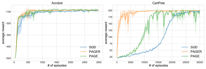
Figure 4: Performance of ${\sf\footnotesize SGD}$, ${\sf\footnotesize PAGER}$ and ${\sf\footnotesize PAGE}$ on benchmark RL tasks.

References

- [1] Alekh Agarwal, Sham M. Kakade, Jason D. Lee, and Gaurav Mahajan. On the Theory of Policy Gradient Methods: Optimality, Approximation, and Distribution Shift. arXiv preprint arXiv:1908.00261, 2020.
- [2] Zeyuan Allen-Zhu, Yuanzhi Li, and Zhao Song. A Convergence Theory for Deep Learning via Over-Parameterization. In Proceedings of International Conference on Machine Learning, 2019.
- [3] Yossi Arjevani, Yair Carmon, John C. Duchi, Dylan J. Foster, Ayush Sekhari, and Karthik Sridharan. Second-order information in non-convex stochastic optimization: Power and limitations. In Proceedings of Thirty Third Conference on Learning Theory, 2020.
- [4] Yossi Arjevani, Yair Carmon, John C Duchi, Dylan J Foster, Nathan Srebro, and Blake Woodworth. Lower bounds for non-convex stochastic optimization. arXiv preprint arXiv:1912.02365, 2019.
- [5] Jonathan Baxter and Peter L. Bartlett. Infinite-horizon policy-gradient estimation. Journal of Artificial Intelligence Research, 2001.
- [6] Dimitri P Bertsekas and John N Tsitsiklis. Gradient convergence in gradient methods with errors. SIAM Journal on Optimization, 2000.
- [7] Yingjie Bi, Haixiang Zhang, and Javad Lavaei. Local and Global Linear Convergence of General Low-rank Matrix Recovery Problems. arXiv preprint arXiv:2104.13348, 2021.
- [8] Doron Blatt, Alfred O. Hero, and Hillel Gauchman. A convergent incremental gradient method with a constant step size. SIAM Journal on Optimization, 2007.
- [9] Jérôme Bolte, Aris Daniilidis, and Adrian Lewis. The Łojasiewicz inequality for nonsmooth subanalytic functions with applications to subgradient dynamical systems. SIAM Journal on Optimization, 2007.
- [10] Jérôme Bolte, Shoham Sabach, and Marc Teboulle. Proximal alternating linearized minimization for nonconvex and nonsmooth problems. Mathematical Programming, 2014.
- [11] Léon Bottou, Frank E Curtis, and Jorge Nocedal. Optimization methods for large-scale machine learning. Siam Review, 2018.
- [12] Greg Brockman, Vicki Cheung, Ludwig Pettersson, Jonas Schneider, John Schulman, Jie Tang, and Wojciech Zaremba. Openai gym. arXiv preprint arXiv:1606.01540, 2016.
- [13] Jingjing Bu, Afshin Mesbahi, Maryam Fazel, and Mehran Mesbahi. LQR through the lens of first order methods: Discrete-time case. arXiv preprint arXiv:1907.08921, 2019.
- [14] Xin Chen, Niao He, Yifan Hu, and Zikun Ye. Efficient Algorithms for Minimizing Compositions of Convex Functions and Random Functions and Its Applications in Network Revenue Management. arXiv preprint arXiv:2205.01774, 2022.
- [15] Ashok Cutkosky and Francesco Orabona. Momentum-based variance reduction in non-convex SGD. In Advances in Neural Information Processing Systems, 2019.
- [16] Aaron Defazio, Francis Bach, and Simon Lacoste-Julien. SAGA: A Fast Incremental Gradient Method With Support for Non-Strongly Convex Composite Objectives. In Advances in Neural Information Processing Systems, 2014.
- [17] Cong Fang, Chris Junchi Li, Zhouchen Lin, and Tong Zhang. SPIDER: Near-Optimal Non-Convex Optimization via Stochastic Path-Integrated Differential Estimator. In Advances in Neural Information Processing Systems, 2018.
- [18] Cong Fang, Zhouchen Lin, and Tong Zhang. Sharp analysis for nonconvex sgd escaping from saddle points. In Proceedings of the Thirty-Second Conference on Learning Theory, 2019.
- [19] Ilyas Fatkhullin and Boris Polyak. Optimizing static linear feedback: Gradient method. SIAM Journal on Control and Optimization, 2021.
- [20] Xavier Fontaine, Valentin De Bortoli, and Alain Durmus. Convergence rates and approximation results for SGD and its continuous-time counterpart. In Conference on Learning Theory, 2021.
- [21] Saeed Ghadimi and Guanghui Lan. Stochastic first-and zeroth-order methods for nonconvex stochastic programming. SIAM Journal on Optimization, 2013.
- [22] Ian Goodfellow, Yoshua Bengio, and Aaron Courville. Deep Learning. The MIT Press, 2016.
- [23] Robert Gower, Othmane Sebbouh, and Nicolas Loizou. SGD for structured nonconvex functions: Learning rates, minibatching and interpolation. In Proceedings of International Conference on Machine Learning, 2021.
- [24] Robert Mansel Gower, Nicolas Loizou, Xun Qian, Alibek Sailanbayev, Egor Shulgin, and Peter Richtárik. SGD: General analysis and improved rates. In Proceedings of International Conference on Machine Learning, 2019.
- [25] Benjamin Grimmer. Convergence rates for deterministic and stochastic subgradient methods without lipschitz continuity. SIAM Journal on Optimization, 2019.
- [26] Mark Schmidt Hamed Karimi, Julie Nutini. Linear convergence of gradient and proximal-gradient methods under the Polyak-Łojasiewicz condition. arXiv preprint arXiv:1608.04636v4, 2016.
- [27] Jia Hu, Congying Han, Tiande Guo, and Tong Zhao. On the Convergence of Stochastic Splitting Methods for Nonsmooth Nonconvex Optimization. arXiv: Optimization and Control, 2021.
- [28] Rie Johnson and Tong Zhang. Accelerating Stochastic Gradient Descent using Predictive Variance Reduction. In Advances in Neural Information Processing Systems, 2013.
- [29] Hamed Karimi, Julie Nutini, and Mark Schmidt. Linear convergence of gradient and proximal-gradient methods under the polyak-Łojasiewicz condition. In Joint European Conference on Machine Learning and Knowledge Discovery in Databases, 2016.
- [30] Ahmed Khaled and Peter Richtárik. Better theory for SGD in the nonconvex world. arXiv preprint arXiv:2002.03329, 2020.
- [31] Guanghui Lan. First-Order and Stochastic Optimization Methods for Machine Learning. Springer Series in the Data Sciences. Springer International Publishing, 2020.
- [32] Lihua Lei, Cheng Ju, Jianbo Chen, and Michael I Jordan. Non-convex Finite-Sum Optimization Via SCSG Methods. In Advances in Neural Information Processing Systems, 2017.
- [33] Tadeusz Ležanski. Gradient methods for minimizing functionals. Mathematische Annalen, 1963.
- [34] Qunwei Li, Yi Zhou, Yingbin Liang, and Pramod K. Varshney. Convergence analysis of proximal gradient with momentum for nonconvex optimization. In Proceedings of International Conference on Machine Learning, 2017.
- [35] Xiao Li, Andre Milzarek, and Junwen Qiu. Convergence of random reshuffling under the Kurdyka-Łojasiewicz inequality. arXiv preprint arXiv:2110.04926, 2021.
- [36] Zhize Li, Hongyan Bao, Xiangliang Zhang, and Peter Richtárik. Page: A simple and optimal probabilistic gradient estimator for nonconvex optimization. arXiv preprint arXiv:2008.10898, 2021.
- [37] Zhize Li and Jian Li. A Simple Proximal Stochastic Gradient Method for Nonsmooth Nonconvex Optimization. In Advances in Neural Information Processing Systems, 2018.
- [38] Stanisław Łojasiewicz. Sur le probleme de la division. Studia Mathematica, 1959.
- [39] Stanislaw Łojasiewicz. A topological property of real analytic subsets. Coll. du CNRS, Les équations aux dérivées partielles, 1963.
- [40] Jincheng Mei, Yue Gao, Bo Dai, Csaba Szepesvari, and Dale Schuurmans. Leveraging non-uniformity in first-order non-convex optimization. In Proceedings of International Conference on Machine Learning, 2021.
- [41] Jincheng Mei, Chenjun Xiao, Csaba Szepesvari, and Dale Schuurmans. On the Global Convergence Rates of Softmax Policy Gradient Methods. In Proceedings of International Conference on Machine Learning, 2020.
- [42] Arkadij Semenovič Nemirovskij and David Borisovich Yudin. Problem complexity and method efficiency in optimization. SIAM Review, 1983.
- [43] Yurii Nesterov and B.T. Polyak. Cubic regularization of newton method and its global performance. Mathematical Programming, 2006.
- [44] Lam M Nguyen, Jie Liu, Katya Scheinberg, and Martin Takáč. Sarah: A novel method for machine learning problems using stochastic recursive gradient. In Proceedings of International Conference on Machine Learning, 2017.
- [45] Lam M. Nguyen, Jie Liu, Katya Scheinberg, and Martin Takáč. SARAH: A Novel Method for Machine Learning Problems Using Stochastic Recursive Gradient. arXiv preprint arXiv:1703.00102, 2017.
- [46] Lam M. Nguyen, Marten van Dijk, Dzung T. Phan, Phuong Ha Nguyen, Tsui-Wei Weng, and Jayant R. Kalagnanam. Finite-Sum Smooth Optimization with SARAH. arXiv preprint arXiv:1901.07648, 2019.
- [47] Matteo Papini, Damiano Binaghi, Giuseppe Canonaco, Matteo Pirotta, and Marcello Restelli. Stochastic variance-reduced policy gradient. In Proceedings of International Conference on Machine Learning, 2018.
- [48] Boris Teodorovich Polyak. Gradient methods for minimizing functionals. Zhurnal vychislitel’noi matematiki i matematicheskoi fiziki, 1963.
- [49] Sashank J Reddi, Ahmed Hefny, Suvrit Sra, Barnabas Poczos, and Alex Smola. Stochastic variance reduction for nonconvex optimization. In Proceedings of International Conference on Machine Learning, 2016.
- [50] Nicolas Roux, Mark Schmidt, and Francis Bach. A Stochastic Gradient Method with an Exponential Convergence _Rate for Finite Training Sets. In Advances in Neural Information Processing Systems, 2012.
- [51] Kevin Scaman, Cedric Malherbe, and Ludovic Dos Santos. Convergence rates of non-convex stochastic gradient descent under a generic lojasiewicz condition and local smoothness. In Proceedings of International Conference on Machine Learning, 2022.
- [52] David Silver, Guy Lever, Nicolas Heess, Thomas Degris, Daan Wierstra, and Martin Riedmiller. Deterministic Policy Gradient Algorithms. In Proceedings of International Conference on Machine Learning, 2014.
- [53] Sharan Vaswani, Francis Bach, and Mark Schmidt. Fast and faster convergence of SGD for over-parameterized models and an accelerated perceptron. In International Conference on Artificial Intelligence and Statistics, 2019.
- [54] Stephen A Vavasis. Complexity issues in global optimization: a survey. In Handbook of global optimization. Springer, 1995.
- [55] Zhe Wang, Kaiyi Ji, Yi Zhou, Yingbin Liang, and Vahid Tarokh. SpiderBoost and Momentum: Faster Variance Reduction Algorithms. In Advances in Neural Information Processing Systems, 2019.
- [56] Rui Yuan, Robert M Gower, and Alessandro Lazaric. A general sample complexity analysis of vanilla policy gradient. arXiv preprint arXiv:2107.11433, 2021.
- [57] Jinshan Zeng, Shikang Ouyang, Tim Tsz-Kit Lau, Shaobo Lin, and Y. Yao. Global convergence in deep learning with variable splitting via the Kurdyka-Łojasiewicz property. arXiv: Optimization and Control, 2018.
- [58] Dongruo Zhou, Pan Xu, and Quanquan Gu. Stochastic nested variance reduction for nonconvex optimization. In Advances in Neural Information Processing Systems, 2018.
- [59] Yi Zhou, Yingbin Liang, and Huishuai Zhang. Understanding generalization error of SGD in nonconvex optimization. Machine Learning, 2021.