Detecting asset price bubbles using deep learning

Abstract

In this paper we employ deep learning techniques to detect financial asset bubbles by using observed call option prices. The proposed algorithm is widely applicable and model-independent. We test the accuracy of our methodology in numerical experiments within a wide range of models and apply it to market data of tech stocks in order to assess if asset price bubbles are present. Under a given condition on the pricing of call options under asset price bubbles, we are able to provide a theoretical foundation of our approach for positive and continuous stochastic asset price processes. When such a condition is not satisfied, we focus on local volatility models. To this purpose, we give a new necessary and sufficient condition for a process with time-dependent local volatility function to be a strict local martingale.

1 Introduction

The study of methodologies for detecting asset price bubbles has attracted an increasing interest over the last years in order to prevent, or mitigate, the financial distress often following their burst. In the context of the martingale theory of bubbles (see among others Cox and Hobson (2005), Loewenstein and Willard (2000), Jarrow et al. (2007), Jarrow et al. (2010), Jarrow et al. (2011a), Biagini et al. (2014), Protter (2013)), the market price of a (discounted) asset represents a bubble if it is given by a strict local martingale. In this framework, detecting an asset price bubble amounts to determine if the stochastic process modelling the discounted asset price is a true martingale or a strict local martingale.

Our contribution is part of a wide range of works on asset price bubbles detection. The problem is tackled within the framework of local volatility models in the papers Jarrow (2016), Jarrow et al. (2011a) and Jarrow et al. (2011b), via volatility estimation techniques. In Fusari et al. (2020), under the joint assumption of no free lunch with vanishing risk (NFLVR) and no-dominance, the authors pursue this goal by looking at the differential pricing between put and call options, with the motivation that traded call and put options reflect price bubbles differently. On the other hand, a nonparametric estimator of asset price bubbles with the only assumption of NFLVR is proposed in Jarrow and Kwok (2021), using a cross section of European option prices. The approach is based on a nonparametric identification of the state-price distribution and the fundamental value of the asset from option data. In Piiroinen et al. (2018), the authors introduce a statistical indicator of asset price bubbles based on the bid and ask market quotes for the prices of put and call options. This methodology is in particular applied to the detection of asset price bubbles for SABR dynamics. Finally, an asymptotic expansion of the right wing of the implied volatility smile is used in Jacquier and Keller-Ressel (2018) to determine the strict local martingale property of the underlying.

In this paper, we propose a method to tackle this issue based on the observation of call option prices and the use of neural networks. We provide a theoretical foundation and a model-free deep learning approach. More precisely, we feed the network with a set of training data whose $i$-th data point consists of analytical call option prices for different strikes $K_{1},\dots,K_{n}$ and maturities $T_{1},\dots,T_{m}$ produced by an underlying process $X^{i}$ with some known dynamics, together with an indicator specifying if $X^{i}$ is a strict local martingale or a true martingale. To assess if a new underlying (possibly corresponding to market data) has a bubble or not, we evaluate the trained neural network at (market) prices of call options on this underlying for strikes $K_{1},\dots,K_{n}$ and maturities $T_{1},\dots,T_{m}$. Slightly changing the algorithm, we are also able to estimate the size of the bubble.

One of the main advantages of our approach is that it does not require the direct estimation of any parameter or quantity related to the asset price process, and that it is model independent. In particular, we show via numerical experiments that our method works not only within a class of models, but also if the network is trained using a certain class of stochastic processes (like local volatility models) and tested within another class (for example, stochastic volatility models). We also test the method with market data associated to assets involved in the new tech bubble burst at the beginning of 2022 (see among others Bercovici (2017), Ozimek (2017), Serla (2017), Sharma (2017)) finding a close match between the output of the network and the expected results.

Our motivation for this method is manifold: on the one hand, the price of call options on a bubbly underlying has an additional term which is added to the usual risk neutral valuation due to a collateral requirement represented by a constant $\alpha\in[0,1]$, see Cox and Hobson (2005) and Theorem 2.4 in our paper. Looking at call option prices, it is then theoretically possible to assess if the underlying has a bubble by identifying the presence of this term. On the other hand, in the case when the underlying price follows a local volatility model, a modified version of Dupire’s formula stated in Theorem 2.3 of Ekström and Tysk (2012) permits to theoretically recover the local volatility function, which is crucial to determine if the process is a strict local martingale or a true martingale, from the observation of call option prices.

In this way we are able to provide a theoretical foundation for our method. In particular, in Theorems 2.10 and 2.22 we prove the existence of a sequence of neural networks approximating a theoretical “bubble detection function” $F$, under the assumption $\alpha<1$ for underlyings given by continuous and positive stochastic processes and in the general case $\alpha\in[0,1]$ for local volatility models. The function $F$ maps from the space ${\mathcal{X}}$ of call option prices as functions of strike and maturity to $\{0,1\}$, being $1$ if and only if the underlying process is a strict local martingale. Several steps are required in order to prove Theorems 2.10 and 2.22. First, we show the existence of the function $F$ introduced above and show that it is measurable with respect to a natural topology on ${\mathcal{X}}$, see Propositions 2.6 and 2.19. In the case when $\alpha=1$, we consider the class of local volatility models under a fairly general assumption on the local volatility function. Specifically, we use some new findings providing a sufficient and necessary condition for a stochastic process with time dependent local volatility function to be a strict local martingale. The main result of this analysis is stated in Theorem 2.17 and is of independent interest, since it is a generalisation of Theorem 8 of Jarrow et al. (2011a). In Propositions 2.7 and 2.21 we then construct a sequence of measurable functions $(F^{n})_{n\geq 1}$ approximating $F$ pointwise, where $F^{n}:\mathbb{R}^{n}\to[0,1]$ takes the prices of a call option with fixed underlying for $n$ different strikes and maturities and outputs the likelihood that the underlying has a bubble according to the observation of these prices. These propositions are then used together with the universal approximation theorem, see Hornik (1991), to prove Theorems 2.10 and 2.22, respectively.

The paper is structured as follows. Section 2 is devoted to the theoretical foundation of our approach. In particular, in Section 2.1 we introduce call option pricing in presence of financial asset bubbles, and in 2.2 we prove existence of the test function $F$ and of its neural network approximation when $\alpha<1$, when the asset price is given by a continuous and positive stochastic process. On the other hand, in Section 2.3 we focus on local volatility models to cover the general case $\alpha\in[0,1]$: in Section 2.3.1 we provide sufficient and necessary conditions for the strict local martingale property of local volatility models, whereas in Section 2.3.2 we give results analogous to the ones in Section 2.2 under this new setting.

In Section 3 we test the performance of our methodology via numerical experiments. Specifically, in Section 3.1 we both feed and test the network within local volatility models, with different, randomly chosen parameters, whereas in Section 3.2 we feed the network with data coming from stochastic volatility models and test it with local volatility models, and vice-versa. In Section 4 we apply our approach to the analysis of three stocks that have been claimed to be affected by a bubble in recent years, namely Nvidia, Apple and Tesla. In Section 5 we present some conclusions.

2 Theoretical foundation

2.1 European call options under asset price bubbles

Let $(\Omega,P,{\mathcal{F}})$ be a probability space endowed with a filtration ${\mathbb{F}}=({\mathcal{F}}_{t})_{t\geq 0}$ satisfying the usual hypothesis. It is well known that the risk-neutral valuation of European options when the underlying asset price has a bubble (i.e., when it is a strict local martingale) does not satisfy the put-call parity, see for example Jarrow et al. (2010). An alternative way to price call options for a bubbly underlying, also supported by market data, has been proposed in Cox and Hobson (2005).

We start with the following definition.

Definition 2.1.

Introduce an underlying given by a continuous, positive stochastic process $X=(X)_{t\geq 0}$, and fix a pricing measure $Q\sim P$ under which $X$ is a local martingale. The price $C^{\alpha,X}(T,K)$ at time $t=0$ of a call option of maturity $T$ and strike $K$ written on $X$ with collateral constant $\alpha\in[0,1]$ is given by

$$C^{\alpha,X}(T,K)=\mathbb{E}^{Q}[(X_{T}-K)^{+}]+\alpha m(T),$$ (1)

where

$$m(T)=X_{0}-\mathbb{E}^{Q}[X_{T}].$$ (2)

The term $m(T)$ in (2) is called the martingale defect of $X$. Note that $m(T)>0$ if $X$ is a strict local martingale bounded from below and $m(T)=0$ if $X$ is a martingale.

Remark 2.2.

Note that if for $t\in[0,T]$ we set

$$C^{\alpha,X}_{t}(T,K):=\mathbb{E}^{Q}[(X_{T}-K)^{+}|\mathcal{F}_{t}]+\alpha m_{t}(T)$$

for $m_{t}(T)=X_{t}-E^{Q}[X_{T}|\mathcal{F}_{t}]$, then $C^{\alpha,X}_{t}(T,K)$, $t\in[0,T]$, is a non-negative local martingale, which equals $(X_{T}-K)^{+}$ at final time. Hence $C^{\alpha,X}_{t}(T,K)$ represents an arbitrage-free price at time $t$ for the call option $(X_{T}-K)^{+}$.

If the market is complete, a financial interpretation of (1)-(2) where $\alpha\in[0,1]$ assumes the meaning of collateral requirement comes from Cox and Hobson (2005), where the following definition is given.

Definition 2.3.

The price at time $t=0$ of a call option $C=(X_{T}-K)^{+}$ of maturity $T$ and strike $K$ written on a continuous, positive underlying $X=(X_{t})_{t\geq 0}$ is the smallest initial value $V_{0}$ of a superreplicating portfolio $V=(V_{t})_{t\geq 0}$ satisfying the admissibility condition

$$V_{t}\geq\alpha(X_{t}-K)^{+}$$ (3)

for all $t\in[0,T],$ where $\alpha\in[0,1]$ is a constant representing the collateral requirement.

Condition (3) is always satisfied when the underlying asset has no bubble. For complete market models we have the following result, given in Cox and Hobson (2005).

Theorem 2.4.

Introduce an underlying given by a continuous, positive stochastic process $X=(X)_{t\geq 0}$, and assume the existence of a unique probability measure $Q\sim P$ under which $X$ is a local martingale. The price according to Definition 2.3 at time $t=0$ of a call option of maturity $T$ and strike $K$ written on $X$ and with collateral requirement $\alpha\in[0,1]$ is given by equation (1).

Such results can be extended to càdlàg processes, see Cox and Hobson (2005).

Remark 2.5.

Under a condition known as no dominance, the price of a call option on a bubbly asset is given by formula (1) with $\alpha=1$ and satisfies the put-call parity, see Theorem 6.2 of Jarrow et al. (2010). Our setting, where $\alpha\in[0,1]$, includes the framework of Jarrow et al. (2010) as a particular case. Moreover, our method does not need to know which value of $\alpha$ is taken to price the option.

2.2 Neural network approximation for collateral $\alpha\in[0,1)$

In this section we fix a collateral constant $\alpha\in[0,1)$ and suppose that the price of a call option is given by (1), with continuous and positive underlying $X$. For the sake of simplicity, from now on we write $C^{X}$ for the call option price. We treat the case $\alpha=1$ in Section 2.3 in the specific setting of local volatility models. Our aim is to find a way of detecting asset price bubbles by using neural networks, as we explain in the sequel. From now on, we fix the “pricing measure” $Q\sim P$.

We start our analysis with the following result.

Proposition 2.6.

Fix a constant $x_{0}>0$. Consider the spaces

$${\mathcal{M}}_{loc}=\bigl{\{}X=(X_{t})_{t\geq 0}\text{ } \text{continuous and positive local martingale on $(\Omega,{\mathcal{F}},Q,{\mathbb{F}})$ {with $X_{0}=x_{0}$}}\bigr{\}}$$

and

$${\mathcal{M}}_{L}=\{\text{$X\in{\mathcal{M}}_{loc}$: $X$ is a strict local martingale}\}.$$ (4)

Introduce the set

$${\mathcal{X}}:=\left\{C^{X}:\text{ }X\in{\mathcal{M}}_{loc}\right\}{\cap C([0,\infty)\times(0,\infty),[0,\infty)})$$ (5)

endowed with the Borel sigma-algebra of ${C([0,\infty)\times(0,\infty),[0,\infty))}$. Then there exists a measurable function $F\colon{\mathcal{X}}\to\{0,1\}$ such that $F(C^{X})=\mathbbm{1}_{\{X\in{\mathcal{M}}_{L}\}}$.

In particular, one can choose

$$F(f):=\mathbbm{1}_{\{\text{there exists $t\geq 0$ such that $\lim_{x\to 0}f(T,x)<X_{0}$ for any $T\geq t$}\}},\quad f\in{\mathcal{X}}.$$ (6)

Proof.

Let $X\in{\mathcal{M}}_{loc}$. From (1) and (2) we get

$$\lim_{K\to 0}C^{X}(T,K)=\lim_{K\to 0}{\mathbb{E}^{Q}[(X_{T}-K)^{+}]}+\alpha m(T)=\mathbb{E}^{Q}[X_{T}]+\alpha(X_{0}-\mathbb{E}^{Q}[X_{T}])=\alpha X_{0}+\mathbb{E}^{Q}[X_{T}](1-\alpha),$$ (7)

by the Dominated Convergence Theorem since $X$ is a supermartingale and therefore integrable for any $t\geq 0$. In particular, since $X$ is a supermartingale, equation (7) implies that it is a strict local martingale if and only if there exists $t>0$ such that

$$\lim_{K\to 0}C^{X}(T,K)<X_{0}\text{ for any {$T\geq t$}}.$$

Therefore, we have

$$F(C^{X})={\mathbbm{1}_{\{X\in{\mathcal{M}}_{L}\}}}\text{ for any $C^{X}\in{\mathcal{X}}$}$$

for $F$ given in (6). In order to prove that $F$ is measurable, note that

$$F(f)=1-\prod_{t\in\mathbb{N}}\bar{F}_{t}(f),\quad f\in{\mathcal{X}},$$

with $\bar{F}_{t}:{\mathcal{X}}\to\{0,1\}$ defined by

$$\bar{F}_{t}(f):=\mathbbm{1}_{\{\lim_{x\to 0}f(t,x)\geq X_{0}\}}=\mathbbm{1}_{\{\lim_{x\to 0}\bar{G}_{t,x}(f)\geq 0\}},\quad t\in\mathbb{N},\quad f\in{\mathcal{X}},$$

where $\bar{G}_{t,x}:{\mathcal{X}}\to\mathbb{R}$ is given by $\bar{G}_{t,x}(f):=f(t,x)-X_{0}$. As $\bar{G}$ is measurable, then also $\lim_{x\to 0}\bar{G}_{t,x}$ is measurable, and hence $\bar{F}_{t}$ and consequently $F$ are also measurable. ∎

We now prove the existence of a sequence of functions $(F^{n})_{n\in\mathbb{N}}$, $F^{n}\colon\mathbb{R}^{n}\to[0,1]$, such that $F^{n}$ approximates, in some way we specify, the function $F$ from (6).

Proposition 2.7.

Define the set

$$A:=[0,\infty)\times(0,\epsilon]$$ (8)

for some fixed $\epsilon>0$.

Let $(T_{n},K_{n})_{n\in\mathbb{N}}$ be a sequence of maturities and strikes such that the set $\{(T_{n},K_{n}),n\in\mathbb{N}\}$ is dense in $A$. Let $\mu$ be a probability measure on ${\mathcal{X}}$ such that there exists a probability measure $\nu$ on ${\mathcal{X}}$ with

$$\nu\left(\left\{f\in{\mathcal{X}}\text{ such that }f(T_{i},K_{i})=g(T_{i},K_{i})\text{ for all $i\in\mathbb{N}$}\right\}\right)>0\quad\text{for any $g\in\operatorname{supp}(\mu)$}.$$ (9)

Then there exists a sequence of functions $(F^{n})_{n\in\mathbb{N}}$, $F^{n}\colon\mathbb{R}^{n}\to[0,1]$ such that

$$\int_{{\mathcal{X}}}\left|F^{n}(g(T_{1},K_{1}),\ldots,g(T_{n},K_{n}))-F(g)\right|^{p}d\mu(g)\xrightarrow[n\to\infty]{}0,$$ (10)

for any $p\in[1,\infty)$, where $F\colon{\mathcal{X}}\to\{0,1\}$ is the function introduced in (6). For fixed $n\in\mathbb{N}$, the function $F^{n}$ can be chosen as follows:

$$F^{n}(c^{n}):=\begin{cases}\frac{1}{\nu\left(S_{n}(c^{n})\right)}\int_{S_{n}(c^{n})}F(f)d\nu(f)\quad&\text{if $\nu\left(S_{n}(c^{n})\right)>0$},\\ 0\quad&\text{otherwise},\end{cases}$$ (11)

$c^{n}\in\mathbb{R}^{n}$, where

$$S_{n}(c^{n}):=\left\{f\in{\mathcal{X}}\text{ such that }f(T_{i},K_{i})=c^{n}_{i}\text{ for all $i=1,\dots,n$}\right\},\quad c^{n}\in\mathbb{R}^{n}.$$ (12)

Proof.

Let $(T_{n},K_{n})_{n\in\mathbb{N}}$ be a sequence of maturities and strikes such that the set $\{(T_{n},K_{n}),n\in\mathbb{N}\}$ is dense in $A$ given in (8). Let $\mu$ be the probability measure on ${\mathcal{X}}$ introduced above and fix $g\in\operatorname{supp}(\mu)$. Also let $\nu$ be a probability measure on ${\mathcal{X}}$ which satisfies (9). For any $n\in\mathbb{N}$, consider the function $F^{n}\colon\mathbb{R}^{n}\to[0,1]$ defined in (11) and set

$$c^{g,n}:=\left(g(T_{1},K_{1}),\dots,g(T_{n},K_{n})\right).$$

We first want to show that

$$F^{n}(c^{g,n})\xrightarrow[n\to\infty]{}F^{\infty}(c^{g,\infty}),$$ (13)

with

$$c^{g,\infty}:=\{g(T_{i},K_{i}),\quad i\in\mathbb{N}\}$$

and

$$F^{\infty}(c^{g,\infty}):=\frac{1}{\nu(S_{\infty}(c^{g,\infty}))}\int_{S_{\infty}(c^{g,\infty})}F(f)d\nu(f),$$

where

$$S_{\infty}(c^{g,\infty}):=\left\{f\in{\mathcal{X}}\text{ such that }f(T_{i},K_{i})=g(T_{i},K_{i})\text{ for all $i\in\mathbb{N}$}\right\}$$

satisfies $\nu(S_{\infty}(c^{g,\infty}))\neq 0$ by (9). Since $S_{n+1}(c^{g,n+1})\subset S_{n}(c^{g,n})$ for any $n\in\mathbb{N}$ and $S_{\infty}(c^{g,\infty})=\bigcap\limits_{n\in\mathbb{N}}S_{n}(c^{g,n})$, we have

$$\mathbb{1}_{S_{n}(c^{g,n})}\xrightarrow[n\to\infty]{}\mathbb{1}_{S_{\infty}(c^{g,\infty})}\quad\text{pointwise}$$ (14)

and

$$\nu\left(S_{n}(c^{g,n})\right)\xrightarrow[n\to\infty]{}\nu\left(S_{\infty}(c^{g,\infty})\right).$$ (15)

By (14) and since $|F|\leq 1$, we can apply the Dominated Convergence Theorem and get

$$\int_{S_{n}(c^{g,n})}F(f)d\nu(f)\xrightarrow[n\to\infty]{}\int_{S_{\infty}(c^{g,\infty})}F(f)d\nu(f).$$ (16)

Putting together (15) and (16), we obtain (13).

Moreover, as the set $\{(T_{n},K_{n}),n\in\mathbb{N}\}$ is dense in $A$ by assumption, $g$ is continuous and every function in ${\mathcal{X}}$ is continuous as well, we have that

$$S_{\infty}(c^{g,\infty})=\left\{f\in{\mathcal{X}}\text{ such that }f(T,K)=g(T,K)\text{ for all $(T,K)\in A$}\right\}.$$

By the definition of $F$ in (6), this implies that $F(f)=F(g)$ for any $f\in S_{\infty}(c^{g,\infty})$, and so $F^{\infty}(c^{g,\infty})=F(g)$. By (13), it thus follows that

$$F^{n}(g(T_{1},K_{1}),\ldots,g(T_{n},K_{n}))\xrightarrow[n\to\infty]{}F(g).$$

We then obtain (10) by the Dominated Convergence Theorem, since $(F^{n})_{n\in\mathbb{N}}$ is bounded by $1$. ∎

Remark 2.8.

Any discrete probability measure $\mu$ on ${\mathcal{X}}$, i.e. any probability measure $\mu$ such that $\operatorname{supp}(\mu)\subseteq{\mathcal{X}}_{0}$ for a countable set ${\mathcal{X}}_{0}\subset{\mathcal{X}}$, satisfies the requirement of Proposition 2.7 that there exists a probability measure $\nu$ on ${\mathcal{X}}$ for which (9) holds. An example is given by

$$\nu:=\frac{1}{\sum_{n\in\mathbb{N}}n^{-2}}\sum_{n\in\mathbb{N}}\delta_{g_{n}}n^{-2},$$

where ${\mathcal{X}}_{0}:=\{g_{n},n\in\mathbb{N}\}$. Indeed, for any $g\in\operatorname{supp}(\mu)$ there exists $n\in\mathbb{N}$ such that $g=g_{n}$, thus

$$\nu\left(\left\{f\in{\mathcal{X}}\text{ such that }f(T_{i},K_{i})=g(T_{i},K_{i})\text{ for all $i\in\mathbb{N}$}\right\}\right)\geq\nu\left(\left\{g_{n}\right\}\right)>0.$$

We now want to approximate the sequence of functions $F^{n}:\mathbb{R}^{n}\to$ defined in (11), and thus the function $F$, by a sequence of neural networks. We start with the formal definition of a neural network, see for example Hornik (1991).

Definition 2.9.

Let $I\subseteq\mathbb{R}$. A neural network $\hat{F}\colon\mathbb{R}^{n}\to I$ is a function

$$\hat{F}(x)=(\psi\circ W_{L}\circ({\sigma}\circ W_{L-1})\circ\cdots\circ({\sigma}\circ W_{1}))(x),\quad x\in\mathbb{R}^{n},$$

with given $L\in\mathbb{N}$, $L\geq 2$, where the inner activation function $\sigma\colon\mathbb{R}\to\mathbb{R}$ is bounded, continuous and non-constant, where the outer activation function $\psi\colon\mathbb{R}\to I$ is invertible and Lipschitz continuous and where $W_{\ell}\colon\mathbb{R}^{N_{\ell-1}}\to\mathbb{R}^{N_{\ell}}$ are affine functions with $N_{1},\ldots,N_{L-1}\in\mathbb{N}$, $N_{0}=n$, $N_{L}=1$.

We then have the following result.

Theorem 2.10.

Fix $p\in[1,\infty)$ and let $(T_{n},K_{n})_{n\in\mathbb{N}}$ be the sequence of maturities and strikes introduced in Proposition 2.7. Also let $\mu$ be a probability measure on ${\mathcal{X}}$ such that there exists a probability measure $\nu$ on ${\mathcal{X}}$ which satisfies (9). Then for any $\epsilon>0$ there exists an $n\in\mathbb{N}$ and a neural network $\hat{F}^{n}\colon\mathbb{R}^{n}\to[0,1]$ such that

$$\left(\int_{\mathcal{X}}|\hat{F}^{n}(g(T_{1},K_{1}),...,g(T_{n},K_{n}))-F(g)|^{p}d\mu(g)\right)^{1/p}<\epsilon.$$

Proof.

Fix $p\in[1,\infty)$ and $\epsilon>0$. By Proposition 2.7 there exists $n\in\mathbb{N}$ such that

$$\int_{\mathcal{X}}|F^{n}(g(T_{1},K_{1}),...,g(T_{n},K_{n}))-F(g)|^{p}d\mu(g)<\left(\frac{\epsilon}{2}\right)^{p},$$ (17)

with $F^{n}$ defined in (11). Let $\psi\colon\mathbb{R}\to[0,1],$ invertible and Lipschitz continuous with Lipschitz constant $K>0$. By the universal approximation theorem, see Hornik (1991), there exists a neural network $\phi^{n}\colon\mathbb{R}^{n}\to\mathbb{R}$ with identity as outer activation function and such that

$$\int_{\mathcal{X}}|\phi^{n}(g(T_{1},K_{1}),...,g(T_{n},K_{n}))-(\psi^{-1}\circ F_{n})(g(T_{1},K_{1}),...,g(T_{n},K_{n}))|^{p}d\mu(g)<\left(\frac{\epsilon}{2K}\right)^{p}.$$

Set now $\hat{F}^{n}:=\psi\circ\phi^{n}$. Then we have

$$\int_{\mathcal{X}}|\hat{F}^{n}(g(T_{1},K_{1}),...,g(T_{n},K_{n}))-F_{n}(g(T_{1},K_{1}),...,g(T_{n},K_{n}))|^{p}d\mu(g)$$

$$\leq K^{p}\int_{\mathcal{X}}|\phi^{n}(g(T_{1},K_{1}),...,g(T_{n},K_{n}))-(\psi^{-1}\circ F_{n})(g(T_{1},K_{1}),...,g(T_{n},K_{n}))|^{p}d\mu(g)<\left(\frac{\epsilon}{2}\right)^{p}.$$ (18)

Therefore it holds

$$\left(\int_{\mathcal{X}}|\hat{F}^{n}(g(T_{1},K_{1}),...,g(T_{n},K_{n}))-F(g)|^{p}d\mu(g)\right)^{1/p}$$

$$\leq\left(\int_{\mathcal{X}}|\hat{F}^{n}(g(T_{1},K_{1}),...,g(T_{n},K_{n}))-F_{n}(g(T_{1},K_{1}),...,g(T_{n},K_{n}))|^{p}d\mu(g)\right)^{1/p}$$

$$\quad+\left(\int_{\mathcal{X}}|F^{n}(g(T_{1},K_{1}),...,g(T_{n},K_{n}))-F(g)|^{p}d\mu(g)\right)^{1/p}$$

$$<\epsilon$$

by (17) and (18). ∎

Remark 2.11.

When $\alpha=1$, we have

$$\lim_{K\to 0}C^{X}(T,K)=\lim_{K\to 0}\mathbb{E}^{Q}[(X_{T}-K)^{+}]+m(T)=X_{0},$$

so the computations illustrated in the proof of Proposition 2.6 do not help detecting the strict local martingale property of $X$. In this case, we prove a neural network approximation focusing on local volatility models.

2.3 The general case $\alpha\in[0,1]$ in the setting of local volatility models

We now include the case $\alpha=1$ in equation (1). In this setting, we focus on the class of local volatility models, i.e., stochastic processes $X=(X_{t})_{t\geq 0}$ such that there exists a risk neutral measure $Q\sim P$ under which $X$ has dynamics

$$dX_{t}=\sigma(t,X_{t})dW_{t},\quad t\geq 0,\quad X_{0}=x>0,$$ (19)

where $W=(W_{t})_{t\geq 0}$ is a one-dimensional $({\mathbb{F}},Q)$-Brownian motion and the function $\sigma$ satisfies the following conditions. In the sequel, martingale and (strict) local martingale are always meant with respect to the probability measure $Q$.

Assumption 2.12.

The function $\sigma:[0,\infty)\times(0,\infty)\to(0,\infty)$ is continuous. Moreover, it is locally Hölder continuous with exponent $1/2$ with respect to the second variable, i.e., for any $L>0$ and any compact set $[0,L]\times[L^{-1},L]$ there exists a constant $C\in[0,\infty)$ such that

$$|\sigma(t,x)-\sigma(t,y)|\leq C|x-y|^{1/2}$$

for all $(t,x,y)\in[0,L]\times[L^{-1},L]^{2}$. Furthermore, there exists a constant $A\in[0,\infty)$ such that $\sigma(t,x)\leq A$ for any $(t,x)\in[0,\infty)\times(0,1]$.

Assumption 2.12 provides existence and uniqueness of a strong solution of (19), see Chapter IX.3 in Revuz and Yor (2013). In particular, we do not require the volatility function to be at most of linear growth in the spatial variable. As stated in the next result, which is Theorem 8 of Jarrow et al. (2011a), this allows $X$ to be a strict local martingale.

Theorem 2.13.

Let $\sigma:[0,\infty)\times(0,\infty)\to(0,\infty)$ be a function satisfying Assumption 2.12. Assume that there exist two functions $\underline{\sigma},\overline{\sigma}:(0,\infty)\to(0,\infty)$, which are continuous and locally Hölder continuous with exponent $1/2$, such that $\underline{\sigma}(x)\leq\sigma(t,x)\leq\overline{\sigma}(x)$ for any $(t,x)\in[0,\infty)\times(0,\infty)$. Let $X=(X_{t})_{t\geq 0}$ be the process in (19). The following holds:

1. If $\int_{c}^{\infty}\frac{y}{\overline{\sigma}^{2}(y)}dy=\infty$ for every $c>0$, then $X$ is a martingale.

2. If there exists $c>0$ such that $\int_{c}^{\infty}\frac{y}{\underline{\sigma}^{2}(y)}dy<\infty$, then $X$ is a strict local martingale.

We now give a generalization of Theorem 2.13 that is useful to provide the theoretical foundation of our methodology in this setting.

2.3.1 Strict local martingale property of local volatility models

Before stating the main result, we give two lemmas.

Lemma 2.14.

Fix $c>0$. Let $\sigma:[0,\infty)\times(0,\infty)\to(0,\infty)$ be a function satisfying Assumption 2.12 and $X=(X_{t})_{t\geq 0}$ be the process in (19). Then $X$ is a strict local martingale if there exist $s,T$ with $0\leq s<T$ and a function $\underline{\sigma}:(0,\infty)\to(0,\infty)$, continuous and locally Hölder continuous with exponent $1/2$, such that:

$$\int_{c}^{\infty}\frac{y}{\underline{\sigma}^{2}(y)}dy<\infty,$$ (20)

$$\underline{\sigma}(x)\leq\sigma(t,x)\text{ for any $(t,x)\in[s,T]\times(0,\infty)$}.$$ (21)

Proof.

Let $0\leq s<T$ and $\underline{\sigma}$ as above. For $x\in(0,\infty)$, define the process $X^{\underline{\sigma},T,s,x}$ to be the unique strong solution of

$$dX^{\underline{\sigma},T,s,x}_{t} =\underline{\sigma}(X^{\underline{\sigma},T,s,x}_{t})dW_{t},\quad s\leq t\leq T,$$

$$X^{\underline{\sigma},T,s,x}_{s} =x.$$

Lemma 9 of Jarrow et al. (2011a) together with the assumption in (21) implies that

$${\mathbb{E}^{Q}}[X_{T}|X_{s}=x]\leq{\mathbb{E}^{Q}}[X^{\underline{\sigma},T,s,x}_{T}]<x,$$

where the last inequality comes from the fact that the process $X^{\underline{\sigma},T,s,x}$ is a strict local martingale for any $(s,x)\in[0,\infty)\times(0,\infty)$ by Theorem 7 of Jarrow et al. (2011a) and (20). ∎

Lemma 2.15.

Fix $c>0$ and $(r,x)\in[0,\infty)\times(0,\infty).$ Let $\sigma:[0,\infty)\times(0,\infty)\to(0,\infty)$ be a function satisfying Assumption 2.12. Denote by $X^{r,x}=(X^{r,x}_{t})_{t\geq r}$ the unique strong solution of the SDE

$$dX^{r,x}_{t} =\sigma(t,X^{r,x}_{t})dW_{t},\quad t\geq r,$$

$$X^{r,x}_{r} =x.$$

Then $X^{r,x}$ is a true martingale if for all $T>r$ there exists a function $\overline{\sigma}^{(T)}:(0,\infty)\to(0,\infty)$, continuous and locally Hölder continuous with exponent $1/2$, such that:

$$\int_{c}^{\infty}\frac{x}{(\overline{\sigma}^{(T)}(x))^{2}}dx=\infty,$$ (22)

$$\overline{\sigma}^{(T)}(x)\geq\sigma(t,x)\text{ for any $(t,x)\in[r,T]\times(0,\infty)$}.$$ (23)

Proof.

Consider $s,T$ such that $T>s\geq r$, and $y\in(0,\infty)$. Define the process $X^{\overline{\sigma},T,s,y}$ to be the unique strong solution of

$$dX^{\overline{\sigma},T,s,y}_{t} =\overline{\sigma}^{(T)}(X^{\overline{\sigma},T,s,y}_{t})dW_{t},\quad s\leq t\leq T,$$

$$X^{\overline{\sigma},T,s,y}_{s} =y.$$

Lemma 9 of Jarrow et al. (2011a) together with the assumption in (23) implies that

$${\mathbb{E}^{Q}}[X^{r,x}_{T}|X^{r,x}_{s}=y]\geq{\mathbb{E}^{Q}}[X^{\overline{\sigma},T,s,y}_{T}]=y,$$

where the last equality holds because the process $X^{\overline{\sigma},T,s,x}$ is a martingale by Theorem 7 of Jarrow et al. (2011a) and (22). Since $X^{r,x}$ is a local martingale and then a supermartingale, we obtain ${\mathbb{E}^{Q}}[X^{r,x}_{T}|X^{r,x}_{s}=y]=y$. Therefore, $X^{r,x}$ is a martingale because $s,T$ and $y$ have been chosen arbitrarily. ∎

In Theorem 2.17 we now provide a sufficient and necessary condition for $X$ to be a true martingale in terms of the local volatility function $\sigma$. To this purpose we need requirements on $\sigma$ which are more restrictive than in Assumption 2.12. However they are satisfied in the most commonly employed models in applications.

Assumption 2.16.

The function $\sigma:[0,\infty)\times(0,\infty)\to(0,\infty)$ satisfies Assumption 2.12 and there exist time points $(T_{n})_{n\geq 0}$, with $T_{0}=0$ and $T_{n+1}>T_{n}$ for any $n\geq 0$, such that $\sigma(\cdot,x)$ restricted to any interval $[T_{n},T_{n+1}]$, $n\geq 0$, is monotone increasing for all $x\in(0,\infty)$ or monotone decreasing for all $x\in(0,\infty)$.

Note that Assumption 2.16 includes the case when $\sigma$ is independent of time or is monotone increasing for all $x\in(0,\infty)$ or monotone decreasing for all $x\in(0,\infty)$ with respect to the time variable.

Theorem 2.17.

Fix $c>0$, and let $\sigma:[0,\infty)\times(0,\infty)\to(0,\infty)$ satisfy Assumption 2.16. Let $X=(X_{t})_{t\geq 0}$ be the process in (19). Then $X$ is a true martingale if and only if

$$\int_{c}^{\infty}\frac{x}{\sigma^{2}(T,x)}dx=\infty\text{ for any $T\in(0,\infty)\setminus B^{\sigma}$,}$$ (24)

with

$$B^{\sigma}:=\left\{T>0:\text{$\sigma(\cdot,x)$ has a local maximum at $T$ for all $x\in(0,\infty)$}\right\}.$$ (25)

Proof.

We start proving that if $X$ is a martingale, then (24) holds. Suppose there exists $T\in(0,\infty)\setminus B^{\sigma}$ such that

$$\int_{c}^{\infty}\frac{x}{\sigma^{2}(T,x)}dx<\infty.$$

Assume first that $T\in(T_{n},T_{n+1})$ for some $n\in\mathbb{N}\cup\{0\}$. Then $\underline{\sigma}(x):=\sigma(T,x)$ is a lower bound for $\sigma$ on the interval $[T,T+\delta]$ (on the interval $[T-\delta,T]$) for some $\delta>0$ if $\sigma(\cdot,x)_{|_{[T_{n},T_{n+1}]}}$ is monotone increasing (decreasing) for all $x\in(0,\infty)$. If $T=T_{n}$ for some $n\in\mathbb{N}$, then $\sigma(\cdot,x)_{|_{[T_{n-1},T_{n}]}}$ must be decreasing $\forall x\in(0,\infty)$ and $\sigma(\cdot,x)_{|_{[T_{n},T_{n+1}]}}$ increasing $\forall x\in(0,\infty)$, as $T\notin B^{\sigma}$. Hence, $\underline{\sigma}(x):=\sigma(T,x)$ is a lower bound on $[T_{n-1},T_{n+1}]$. In any case, $\sigma$ satisfies conditions (20) and (21), thus Lemma 2.14 implies that $X$ is a strict local martingale.

We now prove that if (24) holds, then $X$ is a martingale. For the sake of simplicity, we only consider the case when $\sigma(\cdot,x)_{|_{[0,T_{1}]}}$ is increasing $\forall x\in(0,\infty)$ and $\sigma(\cdot,x)_{|_{[T_{1},\infty)}}$ is decreasing $\forall x\in(0,\infty)$. The proof can be analogously generalized.

Under this assumption, we have that (24) is equivalent to

$$\int_{c}^{\infty}\frac{x}{\sigma^{2}(T,x)}dx=\infty\text{ for any $T>0$, $T\neq T_{1}$.}$$ (26)

We get

$${\mathbb{E}^{Q}}[X_{t}|{\mathcal{F}}_{s}]={\mathbb{E}^{Q}}[X^{s,X_{s}}_{t}|{\mathcal{F}}_{s}]=X_{s},\quad T_{1}<s<t,$$ (27)

where the last equality comes from Lemma 2.15, choosing $r=s$ and $\overline{\sigma}^{(T)}(x):=\sigma(s,x)$ for any $T>s$. We now show that the same holds for $s=T_{1}$. Theorem 2.2 of Ekström and Tysk (2012) states that the functions $C,P:[0,\infty)\times(0,\infty)\to\mathbb{R}^{+}$ defined by

$$C(T,K):={\mathbb{E}^{Q}}[(X_{T}-K)^{+}],\quad P(T,K):={\mathbb{E}^{Q}}[(K-X_{T})^{+}],\qquad(T,K)\in[0,\infty)\times(0,\infty),$$

are continuous with respect to $T$ for any fixed $K>0$. From this and from the put-call parity formula

$$C(T,K)=P(T,K)-K+{\mathbb{E}^{Q}}[X_{T}],\qquad(T,K)\in[0,\infty)\times(0,\infty),$$

it follows that

$$\lim_{t\downarrow T_{1}}{\mathbb{E}^{Q}}[X_{t}]=\lim_{t\downarrow T_{1}}C(t,K)-\lim_{t\downarrow T_{1}}P(t,K)+K=C(T_{1},K)-P(T_{1},K)+K={\mathbb{E}^{Q}}[X_{T_{1}}].$$

Since in our case ${\mathbb{E}^{Q}}[X_{t}]$ is constant for any $t>T_{1}$ by (27), we get ${\mathbb{E}^{Q}}[X_{t}]={\mathbb{E}^{Q}}[X_{T_{1}}]$ for any $t>T_{1}$. This implies that

$${\mathbb{E}^{Q}}[X_{t}|{\mathcal{F}}_{T_{1}}]=X_{T_{1}},\quad T_{1}<t,$$ (28)

because $X$ is a supermartingale. Moreover, again by Lemma 2.15 and using that $\sigma(\cdot,x)_{|_{[0,T_{1}]}}$ is increasing $\forall x\in(0,\infty)$, we get

$${\mathbb{E}^{Q}}[X_{t}|{\mathcal{F}}_{s}]=X_{s},\quad s<t<T_{1}.$$ (29)

Finally, we have that

$${\mathbb{E}^{Q}}[X_{t}|{\mathcal{F}}_{s}]={\mathbb{E}^{Q}}\left[{\mathbb{E}^{Q}}[X_{t}|{\mathcal{F}}_{T_{1}}]|{\mathcal{F}}_{s}\right]={\mathbb{E}^{Q}}[X_{T_{1}}|{\mathcal{F}}_{s}]=X_{s},\quad 0<s<T_{1}\leq t,$$ (30)

where the second equality follows by (28). The last equality holds because $X$ is a supermartingale and ${\mathbb{E}^{Q}}[X_{T_{1}}]={\mathbb{E}^{Q}}[X_{s}]$ for all $s\leq T_{1}$, since the expectation is continuous and constant by (29) for any $s<T_{1}$.

Putting together equations (27), (28), (29) and (30) we get that $X$ is a true martingale.

∎

The results above show that, under some conditions, the behaviour of the volatility for large values of the spatial variable determines if the process $X$ is a strict local martingale, i.e., if it has bubbly dynamics.

In the sequel we use these findings as well as a modified version of Dupire’s equation in Ekström and Tysk (2012) in order to prove the existence of a “bubble detection function” in local volatilities models.

2.3.2 Neural network approximation for local volatility models

We now provide a neural network approximation also for the case $\alpha=1$. To this purpose we first state the general Dupire equation for call options for local volatility models, see Theorem 2.3 of Ekström and Tysk (2012).

Theorem 2.18.

Let $X$ be the process in (19). The price $C^{\alpha,X}(T,K)$ in (1) of a call option on $X$ with strike $K>0$ and maturity $T>0$ with collateral requirement $\alpha\in[0,1]$ is the unique bounded classical solution $C^{\alpha,X}\in C^{1,2}\left((0,\infty)\times(0,\infty)\right)\cap C\left([0,\infty)\times[0,\infty)\right)$ of the equation

$$\begin{cases}\partial_{T}C^{\alpha,X}=\mathcal{L}C^{\alpha,X}-(1-\alpha)\partial_{T}m\qquad\text{for $(T,K)\in(0,\infty)\times(0,\infty)$}\\ C^{\alpha,X}(0,K)=(x-K)^{+}\\ C^{\alpha,X}(T,0)=\mathbb{E}^{Q}[X_{T}]+\alpha m(T),\end{cases}$$ (31)

where $\mathcal{L}$ is the second order differential operator

$$\mathcal{L}=\frac{\sigma^{2}(T,K)}{2}\partial_{KK}$$

and $m$ is the martingale defect of $X$ introduced in (2).

Note that, since the martingale defect $m$ is increasing with respect to time if $X$ is a strict local martingale, then $(1-\alpha)\partial_{T}m>0$ for $\alpha<1$.

Furthermore note that it holds

$$\sigma(T,K)=\sqrt{\frac{1}{2}\frac{\partial_{T}{C^{\alpha,X}}(T,K)}{\partial_{KK}{C^{\alpha,X}}(T,K)}},$$ (32)

if $\partial_{KK}{C^{\alpha,X}}(T,K)>0$ for any $(T,K)\in[0,\infty)\times(0,\infty)$. Namely, the PDE in (31) allows to recover the function $\sigma$ from prices of (possibly collateralized) call options. Together with Theorem 2.13, we use the PDE (31) and (32) for detecting asset price bubbles by looking at prices of call options, by means of neural network approximations. We formalize this in the following.

We now assume that call prices are given by (1) with $\alpha=1$, which is the case that was not covered by the results in Section 2.2. We denote by $C^{X}$ the price given in such a way, with underlying $X$ defined by (19), where $\sigma$ satisfies Assumption 2.16 and

$$\partial_{KK}{C^{X}}(T,K)>0\text{ for any $(T,K)\in[0,\infty)\times(0,\infty)$}.$$ (33)

We prove an equivalent of Proposition 2.6 in the current setting.

Introduce the spaces

$${\mathcal{M}}_{loc}^{locvol}=\{\text{$X=(X_{t})_{t\geq 0}$ with dynamics \eqref{eq:localvolatility}, where $\sigma$ satisfies Assumption \ref{ass:monotone} and \eqref{eq:Sigma}}\},$$

and

$${\mathcal{M}}_{L}^{locvol}=\{\text{$X\in{\mathcal{M}}_{loc}^{locvol}$, $X$ strict local martingale}\}.$$

Consider the set

$${\mathcal{X}}^{locvol}:=\{C^{X}\,:\,X\in{\mathcal{M}}_{loc}^{locvol}\}\subset C^{1,2}([0,\infty)\times(0,\infty),(0,\infty))$$ (34)

endowed with the Borel sigma-algebra of the Fréchet space $C^{1,2}([0,\infty)\times(0,\infty),(0,\infty))$ with topology induced by the countable family of seminorms

$$\|f\|_{i,j,n}:=\sup\left\{|\partial^{(i,j)}_{t,x}f(t,x)|,\text{ }(t,x)\in[0,n]\times[1/n,n]\right\},$$ (35)

for $n\in\mathbb{N}$ and $(i,j)=(0,0),(0,1),(0,2),(1,0).$

Proposition 2.19.

Under Assumption 2.16 there exists a measurable function $F\colon{\mathcal{X}}^{locvol}\to\{0,1\}$ such that $F(C^{X})=\mathbbm{1}_{\{X\in{\mathcal{M}}_{L}^{locvol}\}}$. In particular, one can choose

$$F(f):=\mathbbm{1}_{\left\{\text{ there exists $t\in(0,\infty)\setminus B^{(\partial_{t}f,\partial_{xx}f)}$ such that $\int_{c}^{\infty}x\frac{\partial_{xx}f(t,x)}{\partial_{t}f(t,x)}dx<\infty$}\right\}},\quad f\in{{\mathcal{X}}^{locvol}},$$ (36)

for arbitrary fixed $c>0$ and with

$$B^{(\partial_{t}f,\partial_{xx}f)}:=\left\{T>0:\text{$\sigma:=\sqrt{\frac{1}{2}\frac{\partial_{t}f}{\partial_{xx}f}}$ has a local maximum at $T$ for all $x\in(0,\infty)$}\right\}.$$ (37)

Proof.

We have that ${{\mathcal{X}}^{locvol}}\subset C^{1,2}([0,\infty)\times(0,\infty),(0,\infty))$ by Proposition 2.18. Fix $c>0$, and consider $X\in{\mathcal{M}}_{loc}^{locvol}$ with $C^{X}\in{{\mathcal{X}}^{locvol}}$. Theorem 2.17 implies that for any process $X$ of the form (19) where the local volatility function $\sigma$ satisfies Assumption 2.16 it holds

$$X\in{\mathcal{M}}_{L}^{locvol} \exists t\in(0,\infty)\setminus B^{\sigma}:\int_{c}^{\infty}\frac{x}{\sigma^{2}(t,x)}dx<\infty$$ if and only if , (38)

with $B^{\sigma}$ in (25). Consider now $F\colon{{\mathcal{X}}^{locvol}}\to\{0,1\}$ as in (36). From (32) and (38), it is clear that $F(C^{X})=\mathbbm{1}_{\{X\in{{\mathcal{M}}^{locvol}_{L}\}}}$ for any $C^{X}\in{{\mathcal{X}}^{locvol}}$. We now prove that $F$ is measurable. Fix a volatility function $\sigma$ satisfying Assumption 2.16. First note that, if

$$D^{\sigma,\mathbb{Q}}:=\left(\left\{t>0:\int_{c}^{\infty}\frac{x}{\sigma^{2}(t,x)}dx<\infty\right\}\cap\mathbb{Q}\right)\setminus B^{\sigma}=\emptyset,$$ (39)

then

$$D^{\sigma}:=\left\{t>0:\int_{c}^{\infty}\frac{x}{\sigma^{2}(t,x)}dx<\infty\right\}\setminus B^{\sigma}=\emptyset.$$

Indeed, suppose $D^{\sigma}\neq\emptyset$ and consider $t\in D^{\sigma}$. Then either $t$ is a local minimum for $\sigma(\cdot,x)$ for all $x\in(0,\infty)$ or there exists an interval $I_{t}$ with $t\in I_{t}$ on which $\sigma(\cdot,x)$ is monotone increasing for all $x\in(0,\infty)$ or monotone decreasing for all $x\in(0,\infty)$: in all cases, it is possible to find a positive $\bar{t}\in\mathbb{Q}\setminus B^{\sigma}$ such that $\int_{c}^{\infty}\frac{x}{\sigma^{2}(\bar{t},x)}dx<\infty$, hence $D^{\sigma,\mathbb{Q}}\neq\emptyset$.

Then we can write

$$F(f)=1-\prod_{t\in\mathbb{Q}\cap\left((0,\infty)\setminus B^{(\partial_{t}f,\partial_{xx}f)}\right)}(1-F_{t}(f))=1-\prod_{t\in\mathbb{Q}\cap(0,\infty)}(1-F_{t}(f)\mathbb{1}_{\left\{t\notin B^{(\partial_{t}f,\partial_{xx}f)}\right\}}),$$ (40)

$f\in{{\mathcal{X}}^{locvol}}$, with $B^{(\partial_{t}f,\partial_{xx}f)}$ as in (37) and where $F_{t}\colon{{\mathcal{X}}^{locvol}}\to\{0,1\}$ is defined by

$$F_{t}(f):=\mathbbm{1}_{\left\{\int_{c}^{\infty}x\frac{\partial_{xx}f(t,x)}{\partial_{t}f(t,x)}dx<\infty\right\}},\quad f\in{{\mathcal{X}}^{locvol}},$$ (41)

for any $t>0$. Note that for any $t\in\mathbb{Q}\cap(0,\infty)$ and any $\delta\in(0,t)$ we have

$$\mathbb{1}_{\left\{t\notin B^{(\partial_{t}f,\partial_{xx}f)}\right\}}=1-\prod_{x\in\mathbb{Q}\cap(0,\infty)}\prod_{s\in\mathbb{Q}\cap(0,\delta)}\mathbb{1}_{\left\{\frac{\partial_{t}f(t-s,x)}{\partial_{xx}f(t-s,x)}<\frac{\partial_{t}f(t,x)}{\partial_{xx}f(t,x)}\right\}}\mathbb{1}_{\left\{\frac{\partial_{t}f(t+s,x)}{\partial_{xx}f(t+s,x)}<\frac{\partial_{t}f(t,x)}{\partial_{xx}f(t,x)}\right\}},$$

which is measurable. Moreover, we can write $F_{t}=\hat{F}\circ\tilde{F}_{t}$, where the operator $\tilde{F}_{t}\colon{{\mathcal{X}}^{locvol}}\to C\left((0,\infty),(0,\infty)\right)$ is given by

$$\tilde{F}_{t}(f):=I_{d}\cdot\frac{\partial_{xx}f(t,\cdot)}{\partial_{t}f(t,\cdot)}$$

for any $t>0$, with $I_{d}(x)=x$, and $\hat{F}:C\left((0,\infty),(0,\infty)\right)\to\{0,1\}$ equal to

$$\hat{F}(g)=\mathbbm{1}_{\{\int_{c}^{\infty}g(x)dx<\infty\}}.$$

The space $C\left((0,\infty),(0,\infty)\right)$ is a Fréchet space equipped with the Borel sigma-algebra with respect to the topology induced by the family of seminorms

$$\|g\|_{m}:=\sup\left\{|g(x)|,\text{ }x\in[1/m,m]\right\}$$ (42)

for $m\in\mathbb{N}$. Note that $\tilde{F}_{t}$ is well defined for any $t>0$ by (33) and by (32), since $\sigma$ is strictly positive. Moreover, $\tilde{F}_{t}$ is measurable for all $t>0$ because it is continuous with respect to the uniform convergence on compact sets away from zero induced by the topologies of the Fréchet spaces $C^{1,2}([0,\infty)\times(0,\infty),(0,\infty))$ on ${{\mathcal{X}}^{locvol}}$ and $C\left((0,\infty),(0,\infty)\right)$ with the seminorms in (35) and (42), respectively.
Coming now to $\hat{F}$, it can be written as

$$\hat{F}(g)=\mathbbm{1}_{\{I(g)<\infty\}}$$

where $I:C\left((0,\infty),(0,\infty)\right)\to[0,\infty]$ is the integral operator

$$I(g)=\int_{c}^{\infty}g(x)dx,\quad g\in C\left((0,\infty),(0,\infty)\right).$$

Clearly, $I=\lim_{k\to\infty}I_{k}$, where the functions $I_{k}:C\left((0,\infty),(0,\infty)\right)\to[0,\infty)$ with

$$I_{k}(g):=\int_{c}^{k}g(x)dx,\quad g\in C\left((0,\infty),(0,\infty)\right),\quad k\in\mathbb{N},$$

are measurable because the operator $g\to\int_{c}^{k}g(x)dx$ is continuous for any finite $k$. Then $I$ is measurable and $\hat{F}$ as well.

The function $F_{t}$ in (41) is thus measurable for every $t>0$ since it is the composition of measurable functions. Hence, the function $F$ is measurable by (40).

∎

Remark 2.20.

The assumption that $\partial_{KK}{C^{X}}(T,K)>0$ for any $(T,K)\in[0,\infty)\times(0,\infty)$ in (33) is equivalent to

$$\partial_{T}{C^{X}}(T,K)>0,\quad(T,K)\in[0,\infty)\times(0,\infty),$$

which is usually satisfied for the observed market prices.

The above conditions are satisfied, for instance, if $X_{T}$ admits a strictly positive density $g_{T}^{X}:\mathbb{R}_{+}\to\mathbb{R}_{+}$ for any $T\geq 0$. Indeed, under this assumption it holds that

$$\partial_{KK}{C^{X}}(T,K)=\partial_{KK}\int_{K}^{\infty}(x-K)g_{T}^{X}(x)dx=g_{T}^{X}(K)>0$$

for any $K>0$.

We now give a result analogous to Proposition 2.7. The proof is follows the same steps.

Proposition 2.21.

Define the set

$$A=[0,\infty)\times[C,\infty)$$

for some fixed $C>0$. Let $(T_{n},K_{n})_{n\in\mathbb{N}}$ be a sequence of maturities and strikes such that the set $\{(T_{n},K_{n}),n\in\mathbb{N}\}$ is dense in $A$. Let $\mu$ be a probability measure on the space ${\mathcal{X}}^{locvol}$ introduced in (34) such that there exists a probability measure $\nu$ on ${{\mathcal{X}}^{locvol}}$ with

$$\nu\left(\left\{f\in{\mathcal{X}}^{locvol}\text{ such that }f(T_{i},K_{i})=g(T_{i},K_{i})\text{ for all $i\in\mathbb{N}$}\right\}\right)>0\quad\text{for any $g\in\operatorname{supp}(\mu)$}.$$ (43)

Then there exists a sequence of functions $(F^{n})_{n\in\mathbb{N}}$, $F^{n}\colon\mathbb{R}^{n}\to[0,1]$ such that

$$\int_{{\mathcal{X}}^{locvol}}\left|F^{n}(g(T_{1},K_{1}),\ldots,g(T_{n},K_{n}))-F(g)\right|^{p}d\mu(g)\xrightarrow[n\to\infty]{}0,$$

for any $p\in[1,\infty)$, where $F\colon{\mathcal{X}}^{locvol}\to\{0,1\}$ is the function introduced in (36). For fixed $n\in\mathbb{N}$, the function $F^{n}$ can be chosen as follows:

$$F^{n}(c^{n}):=\begin{cases}\frac{1}{\nu\left(S_{n}(c^{n})\right)}\int_{S_{n}(c^{n})}F(f)d\nu(f)\quad&\text{if $\nu\left(S_{n}(c^{n})\right)>0$},\\ 0\quad&\text{otherwise},\end{cases}$$

$c^{n}\in\mathbb{R}^{n}$, where

$$S_{n}(c^{n}):=\left\{f\in{\mathcal{X}}^{locvol}\text{ such that }f(T_{i},K_{i})=c^{n}_{i}\text{ for all $i=1,\dots,n$}\right\},\quad c^{n}\in\mathbb{R}^{n}.$$ (44)

We then have the following result. The proof follows the same steps as for Theorem 2.10.

Theorem 2.22.

Fix $p\in[1,\infty)$ and let $(T_{n},K_{n})_{n\in\mathbb{N}}$ be the sequence of maturities and strikes introduced in Proposition 2.21. Also let $\mu$ be a probability measure on ${\mathcal{X}}^{locvol}$ such that there exists a probability measure $\nu$ on ${\mathcal{X}}$ which satisfies (43). Then for any $\epsilon>0$ there exists an $n\in\mathbb{N}$ and a neural network $\hat{F}^{n}\colon\mathbb{R}^{n}\to[0,1]$ such that

$$\int_{{\mathcal{X}}^{locvol}}|\hat{F}^{n}(g(T_{1},K_{1}),...,g(T_{n},K_{n}))-F(g)|^{p}{d\mu(g)}<\epsilon.$$

3 Numerical experiments

In Section 2 we have provided a theoretical foundation for the bubble detection methodology explained in the introduction. The method does not require any parameter estimation related to the asset price, and it is model independent when $\alpha<1$. Fixing $\alpha=1$, we now show via numerical experiments that our approach works not only within a class of models, but also if the network is trained using a certain class of stochastic processes (like local volatility models) and tested within another class (for example, stochastic volatility models). We also test the method with market data associated to assets involved in the new tech bubble burst at the beginning of 2022 (see among others Bercovici (2017), Ozimek (2017), Serla (2017), Sharma (2017)) finding a close match between the output of the network and the expected results.

Remark 3.1.

We show the results for a collateral constant $\alpha=1$ because this is the most common choice in the literature, see for example Dias et al. (2020), Heston et al. (2007) and Jarrow et al. (2010). For completeness, we have repeated the same tests for $\alpha=\frac{1}{2}$ finding not inferior accuracies.

3.1 Local volatility models

First, we consider a displaced CEV process $(X_{t})_{t\geq 0}$ with dynamics

$$dX_{t}=\sigma\cdot(X_{t}+d)^{\beta}dW_{t},\quad t\geq 0,\quad X_{0}=x_{0}>0,$$ (45)

where $(W_{t})_{t\geq 0}$ is a one-dimensional standard Brownian motion and $\sigma,\beta,d>0$.

Proposition 3.2.

The SDE (45) has a unique strong solution, which is a true martingale if and only if $\beta\leq 1$.

Proof.

When $d=0$, the SDE (45) admits a unique strong solution since the function $\sigma(x)=x^{\beta}$, $x>0$, satisfies Assumption 2.12. A process $X$ with dynamics given by (45) for general $d>0$ is of the form $X_{t}=Y_{t}-d$, $t\geq 0$, where $Y$ is the unique strong solution of (45) with $d=0$ and $Y_{0}=X_{0}+d$. By Theorem 2.17, $Y$ is a true martingale if and only $\beta\leq 1$, and thus the same holds for $X$. ∎

The proof of the above proposition shows that all the results of Section 2 also apply to (45), even if $X$ is in general not positive but only bounded from below.

Based on Proposition 3.2, we now use neural networks in order to detect if a process satisfying (45) has bubbly dynamics, by looking at the prices of some call options with this process as the underlying. Once we have generated the training data, we are then left with a supervised learning problem. Following Jarrow et al. (2010), we set $\alpha=1$ in (1) from now on.

3.1.1 Random displacement

As a first experiment, we work with $n_{train}\in\mathbb{N}$ different underlyings, all following (45) with fixed $\sigma>0$ and different, randomly chosen parameters $d$ and $\beta$. In particular, for any $i=1,\dots,n_{train}$, the underlying $X^{i}$ has displacement $d_{i}$ uniformly distributed in an interval $[0,D]$ for given $D>0$ and strictly positive exponent $\beta_{i}$. We let $\beta_{i}$ be uniformly distributed in an interval $(a,1]$ with $a\in(0,1)$ in $n_{train}/2$ cases and in an interval $(1,A)$ with $A>1$ for the other $n_{train}/2$ cases, so that we consider $n_{train}/2$ true martingales and $n_{train}/2$ strict local martingales. We also fix strikes $0<K_{1}<\dots<K_{m}$ and maturities $0<T_{1}<\dots<T_{l}$.

The training data are then constituted by an $n_{train}\times(m\cdot l+2)$-matrix whose $i$-th row consists of $l\cdot m$ call prices for all the strikes and maturities above, with respect to the underlying $X^{i}$, and the value of the martingale defect $\mathbb{E}[X^{i}_{T_{l}}]-X^{i}_{0}$ for final time $T_{l}$ and the indicator $\mathbb{1}_{\{X^{i}\text{ is a strict local martingale}\}}$. Note that both the values of the calls and the martingale defect can be computed analytically, as indicated for example in Lindsay and Brecher (2012).

We use the data introduced above to train a neural network with two hidden layers and ReLu activation function to estimate if the processes are strict local martingales or true martingales, as well as the martingale defect. For the first case, we choose a Softmax activation function for the output layer and categorical cross entropy loss function. We use an Adam optimization algorithm, as an extension to stochastic gradient descent. We then test the network with a number of test data $n_{test}$, repeating the procedure described above with same parameters. As metrics of the performance of the algorithm, we consider the frequency with which it can predict if the underlying is a strict local martingale. Furthermore, we compute the $R^{2}$ coefficient of determination score for what regards the computation of the martingale defect as given by

$$1-\frac{\sum_{i=1}^{n_{test}}(y_{i}-f_{i})^{2}}{\sum_{i=1}^{n_{test}}(y_{i}-\bar{y})^{2}},$$

where $y_{i}$ and $f_{i}$, $i=1,2,\dots,n$, are the true and predicted values, respectively, and $\bar{y}$ is the average of the true values. The best possible score is therefore 1.

We choose $n_{train}=100000$, $n_{test}=2000$, $a=0.5$, $A=3$, $D=0.2$, $\sigma=0.2$, $X_{0}=2$, $51$ equally spaced strikes from $K_{1}=1.8$ to $K_{m}=2.3$ and $100$ equally spaced maturities from $T_{1}=1$ to $T_{l}=2$.

• We get an accuracy of $98.61\%$ for the training data and $98.54\%$ for the test data for what regards the detection of bubbles.

• In the test phase, we get an $R^{2}$ coefficient of determination score of $0.994$ for what regards the computation of the martingale defect.

We now aim to further increase the accuracy of our results, without increasing the number of input and test data and of the option prices observed, based on the following ansatz. Looking at equation (1) we note that, if $\alpha>0$, the price of a call option in presence of a bubble diverges from the one without bubble by a term proportional to the martingale defect $m(T)=X_{0}-\mathbb{E}^{Q}[X_{T}]$. This term has a big impact on the price of the option when $C(T,K)$ in (1) is small, i.e., for large values of the strike $K$. Based on this intuition, we consider higher values for $K$ and shift our strike interval from $[1.8,2.3]$ to $[3.5,4]$, considering the same number of strikes. All the other parameters are as indicated above. We note indeed an enhancement of the performance. In particular:

• We get an accuracy of $99.95\%$ both for the training and test data for what regards the detection of bubbles.

• In the test phase, we get an $R^{2}$ coefficient of determination score of $0.999$ for what regards the computation of the martingale defect.

3.1.2 Train with no displacement, test with a strictly positive displacement

We now repeat the experiment described in Section 3.1.1 with the difference that this time the displacements are not random, and they differ from training and testing. In particular, we train and test the network with data generated by an underlying in (45) with $d=0$ and $d=0.5$, respectively. In this way, we can check if the network is able to detect bubbles also when it is trained and tested with data coming from processes having shifted dynamics. All the other parameters are the same as in Section 3.1.1. Using $51$ equally spaced strikes from $K_{1}=1.8$ to $K_{m}=2.3$, we observe the following results:

• We get an accuracy of $99.82\%$ for the training data and $80.70\%$ for the test data for what regards the detection of bubbles.

• In the test phase, we get an $R^{2}$ coefficient of determination score of $0.9$ for what regards the computation of the martingale defect.

We observe a smaller accuracy than in the first case: this can be expected because of the shifted dynamics of the underlying processes that produce the prices to train and test the network, respectively. Note that the displacement we use to test the network is bigger than the biggest possible displacement in the first experiment.

Shifting the interval of strikes from $[1.8,2.3]$ to $[3.5,4]$ increases the performance indicators also in this case. In particular:

• We get an accuracy of $99.99\%$ for the training data and $86.20\%$ for the test data for what regards the detection of bubbles.

• In the test phase, get an $R^{2}$ coefficient of determination score of $0.94$ for what regards the computation of the martingale defect.

If we now instead train the network with displacement $d=0.5$ and test with $d=0$, we observe the following:

• For what regards the training data, we get an accuracy of $98.7\%$ for strikes in $[1.8,2.3]$ and $99.99\%$ for strikes in $[3.5,4]$;

• For the test, we get an accuracy of $93.0\%$ for $K\in[1.8,2.3]$ and $95.45\%$ for strikes in $[3.5,4]$;

• For what concerns the computation of the martingale defect, we get an $R^{2}$ coefficient of determination score of $0.93$ for strikes in $[1.8,2.3]$ and $0.96\%$ for strikes in $[3.5,4]$.

In all the experiments, the accuracy of the results gets smaller if we decrease the number of strikes or the number of maturities, keeping the intervals the same.

3.2 Stochastic volatility models

As an extension of the setting of Section 3.1, we now include stochastic volatility models into our numerical experiments. In particular, we check how our methodology works when the network is fed with data coming from stochastic volatility processes and tested looking at local volatility models, and vice-versa. Since the nature of the two classes of models is deeply different, this analysis constitutes a robust test for our methodology.

In particular, we consider the SABR model and the class of stochastic volatility models introduced in Sin (1998). The SABR volatility model $F=(F_{t})_{t\geq 0}$ is defined as the unique strong solution of the SDE

$$dF_{t} =\sigma_{t}(F_{t})^{\gamma}dW_{t},\qquad t\geq 0,$$ (46)

$$d\sigma_{t} =\alpha\sigma_{t}dZ_{t},\qquad t\geq 0,$$ (47)

with initial value $F_{0}>0$, initial volatility $\sigma_{0}>0$, exponent $\gamma>0$ and volatility of the volatility $\alpha>0$. Here $W$ and $Z$ are Brownian motions with correlation $\rho\in[-1,1]$.

A class of stochastic volatility models of the form

$$dY_{t}=\sigma_{1}v_{t}^{\alpha}Y_{t}dB^{1}_{t}+\sigma_{2}v^{\alpha}_{t}Y_{t}dB_{t}^{2},\quad t\geq 0,$$ (48)

$$dv_{t}=a_{1}v_{t}dB^{1}_{t}+a_{2}v_{t}dB_{t}^{2}+\kappa(L-v_{t})dt,\quad t\geq 0,\quad v_{0}=1,$$ (49)

is considered in Sin (1998), with $\alpha,\kappa,L\in\mathbb{R}^{+}$ and $\sigma_{1},\sigma_{2},a_{1},a_{2},a_{3}\in\mathbb{R}$. It is well known that $Y$ is a strict local martingale if and only if $a_{1}\sigma_{1}+a_{2}\sigma_{2}>0$, see Sin (1998). From now on, we call (48)-(49) the Sin model. It can be noted that, when $\gamma=1$, the SABR model is a particular case of the Sin model, and is a strict local martingale if and only if $\rho>0$.

The call prices for the SABR model admit an analytical approximation, see for example Piiroinen et al. (2018). For the Sin model, on the other hand, we are not aware of any way to analytically compute or approximate the prices, so we rely on Monte-Carlo approximations with $200000$ simulations and time step $0.01$.

We take $61$ maturities equally spaced from $T_{1}=2$ to $T_{l}=5$ and, as in Section 3.1, two groups of $100$ equally spaced strikes: one from $K_{1}=1$ to $K_{m}=3.5$ and one from $K_{1}=3$ to $K_{m}=5.5$. We consider three different classes of processes for the underlying, in all cases with initial value $X_{0}=2$:

• A set of displaced CEV models with same specifications as in Section 3.1, that is, in particular, with randomly varying exponent and displacement;

• A set of SABR models (46)-(47) with parameters $\alpha=0.5$, $\gamma=1$ and $\sigma_{0}=1$. We let the correlation $\rho$ between the process and the volatility be randomly chosen and a priori different for any underlying: in particular, we set it to be uniformly distributed in $[-0.8,0]$ in half of the cases (the ones where the underlying is a true martingale) and in $(0,0.8]$ in the other half of the cases (the ones where the underlying is a strict local martingale).

• A set of Sin models (48)-(49) with parameters $v_{0}=0.5$, $\alpha=1$, $\kappa=0$, $\sigma_{2}=-0.5$, $a_{1}=1.8$ and $a_{2}=1.2$. We let $\sigma_{1}$ be randomly chosen and a priori different for any underlying: specifically, it is uniformly distributed in $[0,1/3]$ in half of the cases (the ones where the underlying is a true martingale) and in $(1/3,1]$ in the other half of the cases (the ones where the underlying is a strict local martingale).

As a benchmark for our following investigation, for which training and test sets will consist of prices generated by underlying coming from different classes of models, Table 1 shows the accuracy in the training and test phases when we both train and test the neural network with any of the three models above. For any class of models, we consider $2000$ underlyings for the training set and $1000$ for the test set. Half of the them are true martingales and half strict local martingales.

	Displaced CEV	Sin	SABR
Strikes in $[1,3.5]$	$a_{train}=98.5\%$, $a_{test}=98.2\%$	$a_{train}=99.8\%$, $a_{test}=99.6\%$	$a_{train}=94.4\%$, $a_{test}=94.8\%$
Strikes in $[3,5.5]$	$a_{train}=99.6\%$, $a_{test}=99.2\%$	$a_{train}=99.8\%$, $a_{test}=99.7\%$	$a_{train}=98.3\%$, $a_{test}=98.4\%$

Table 1: Accuracy on the training set ($a_{train}$) and on the test set ($a_{test}$) when the algorithm to identify bubbles is both trained and tested with one single family of models: the three investigated cases are displaced CEV, Sin model and SABR model.

We now mix the models for training and testing. First, to investigate the performance of our method when trained on stochastic volatility processes and tested on local volatility models, we test the algorithm looking at the prices generated by the set of displaced CEV models, for three different training sets: one constituted exclusively from data coming from the SABR model, one only from the Sin model and one from both of them. In all the three cases, we take a training set consisting of call prices given by $2000$ different underlyings and a test set constituted of call prices for $1000$ underlyings. In both cases, half of the underlyings are true martingales and half strict local martingales. When both the Sin and the SABR models are used for training, the training set is equally split between the two cases. Table 2 shows the accuracy we get on the training set (this is denoted by $a_{train}$) and on the test set (denoted $a_{test}$) in the different cases.

	Only SABR	Only Sin	Both SABR and Sin
Strikes in $[1,3.5]$	$a_{train}=97.2\%$, $a_{test}=67.2\%$	$a_{train}=99.6\%$, $a_{test}=50.0\%$	$a_{train}=93.5\%$, $a_{test}=75.0\%$
Strikes in $[3,5.5]$	$a_{train}=99.5\%$, $a_{test}=87.3\%$	$a_{train}=99.7\%$, $a_{test}=78.3\%$	$a_{train}=98.0\%$, $a_{test}=83.2\%$

Table 2: Accuracy on the training set ($a_{train}$) and on the test set ($a_{test}$) when the algorithm to identify bubbles is tested looking at call prices generated by displaced CEV models, for two different sets of strikes and three different training sets.

In all cases, we see that looking at prices of out-of-the-money options improves the performance, as in Section 3.1. The only case when the algorithm is not able to identify strict local martingales for the class of displaced CEV processes is when the training set consists of prices generated by the class of Sin models, and at-the-money strikes. A deeper look shows that, in this setting, the algorithm labels all displaced CEV underlyings as strict local martingales. Taking bigger strikes, the accuracy of the algorithm considerably increases to $78.7\%$. For both the sets of strikes, the accuracy is bigger when training with the SABR model than with the Sin model. A possible explanation is that the SABR model can be seen as a generalization of the CEV model with stochastic volatility. Moreover, when considering the smaller set of strikes, splitting the training set into the two sets of SABR and Sin processes enhances the performance on the test set with respect to both cases, when we train with only one set of processes, at the expenses of the performance on the training set. In this case, it seems that training with more variety of models makes the algorithm more robust.

We then move to test our methodology looking at the prices generated by the class of SABR models, again for three different training sets: the first two sets consist of call prices generated by the displaced CEV models and by the Sin models, respectively, and the third one of prices generated by both of them. In this way, we complete our investigation: the first case regards training with local volatility and testing with stochastic volatility, the second one concerns both training and testing with stochastic volatility, whereas the third one studies if a combination of training from local and stochastic volatility can be beneficial when looking at a stochastic volatility model. The results are summarized in Table 3.

	Only displaced CEV	Only Sin	Both displaced CEV and Sin
Strikes in $[1,3.5]$	$a_{train}=99.1\%$, $a_{test}=50.0\%$	$a_{train}=99.4\%$, $a_{test}=68.0\%$	$a_{train}=97.3\%$, $a_{test}=92.2\%$
Strikes in $[3,5.5]$	$a_{train}=99.4\%$, $a_{test}=50.0\%$	$a_{train}=99.5\%$, $a_{test}=88.5\%$	$a_{train}=98.5\%$, $a_{test}=95.7\%$

Table 3: Accuracy on the training set ($a_{train}$) and on the test set ($a_{test}$) when the algorithm to identify bubbles is tested looking at data coming from the SABR model, for two different sets of strikes and three different training sets.

As above, looking at bigger strikes we get a bigger accuracy in all cases. Moreover, for both the groups of strikes, training with a combination of data coming from a stochastic volatility model and from a local volatility model increases the accuracy in the test for the SABR model at the expenses of the accuracy in the training set: this suggests that training with higher variety of data makes our methodology more robust. On the other hand, training only with data coming from the displaced CEV processes does not help guessing the strict local martingale property of the SABR processes: in particular, the algorithm always identifies all the processes as strict local martingales. Comparing this case with Table 2 we see that our methodology works fairly good if we train with the SABR models and try to label the CEV models, but not vice-versa.

Concluding, the above results show that, in particular when combining different classes of processes in the training phase, our methodology still works when including stochastic volatility models, even if the results are (not surprisingly) less accurate than when we consider local volatility models for both training and testing.

4 Analysis on market data: detecting tech stocks bubbles

We now use our methodology to detect if some tech stocks have been affected by an asset price bubble in last years. In particular, we focus on Nvidia Corporation (NVDA), Apple Inc. (AAPL) and Tesla Inc. (TSLA). These companies have experienced in the last years a boom, followed by a contraction at the beginning of 2022, as it can also be seen by the prices plots in Figures 1, 2 and 3. This has brought many financial analysts to claim the presence of a new tech bubble, after the dot com mania of the late 1990s (see for example Bercovici (2017), Ozimek (2017), Serla (2017), Sharma (2017)).

Let $S^{i}_{t_{i}}$ be the value at time $t_{i}$ of a stock $i\in\{\text{NVDA},\text{AAPL},\text{TSLA}\}$. In order to assess if a bubble is present at $t_{i}$, we consider the call option market prices $C^{i}_{1},\dots,C^{i}_{n_{i}}$ at $t_{i}$ for some maturities $T^{i}_{1},\dots,T^{i}_{n_{i}}$ and some strikes $K^{i}_{1},\dots,K^{i}_{n_{i}}$. We then train a neural network as in Sections 3.1 and 3.2, by using theoretical call option prices written on a class of SABR models and displaced CEV models as done in Section 3.2, for maturities $T^{i}_{1},\dots,T^{i}_{n_{i}}$, strikes $K_{1},\dots,K^{i}_{n_{i}}$ and initial value of the underlying $S^{i}$. After the training phase, we feed the network with the realized call market prices $C^{i}_{1},\dots,C^{i}_{n_{i}}$, in order to assess if the underlying $i$ has a bubble or not. The families of SABR models and displaced CEV models used to train the network are identified by the following parameters:

• For the SABR models (46)-(47) we set $\gamma=1$, in order to be able to compute the call prices analytically. We let $\sigma_{0}$ and $\alpha$ be both uniformly distributed in $[0.1,0.9]$. Moreover, we let $\rho$ be uniformly distributed in $[-0.9,0]$ in half cases (the ones where the underlying is a true martingale) and in $(0,0.9]$ in the other half of cases (the ones where the underlying is a strict local martingale).

• For the displaced CEV models (45), we let the volatility $\sigma$ and the displacement $d$ be uniformly distributed in $[0.1,0.9]$ and $[0,2]$, respectively. Moreover, we let the exponent $\beta$ be uniformly distributed in $[0.1,1]$ in half cases (the ones where the underlying is a true martingale) and in $(1,1.3]$ in the other half of cases (the ones where the underlying is a strict local martingale).

Note that in the models specification above we take randomly chosen parameters in order to increase the variety of the training data and then the robustness of our methodology.

We now state our findings for the three underlyings.

4.0.1 Nvidia Corporation

The advanced semiconductor manufacturer Nvidia Corp. has seen its shares rocketing to huge heights in last years. From January 2016 to its peak in late November 2021, Nvidia’s closing stock prices boosted their value by about $4600\%$. This seems to point to a bubble in Nvidia stock, see for example Kolakowski (2019).

We apply our methodology in order to check for the presence of a bubble from January 2016 to July 2022, on a six-monthly basis. In Figure 1 we plot the price evolution of the asset with the dates when we use our methodology to detect if a bubble is present. In particular, for each date the algorithm outputs a probability $P_{b}$ for the presence of a bubble. Different colors of the lines correspond to different values of $P_{b}$. We list these findings in more details in the following, in terms of the evolution of $P_{b}$.

• No bubble is detected from January 2016 to July 2017: in particular, $P_{b}$ is equal to $0.01\%$ in January 2016, $1\%$ in July 2016 and January 2017, and $2\%$ in July 2017.

• Our methodology detects a bubble in 2018: in particular, $P_{b}=85\%$ in January 2018 and $P_{b}=99\%$ in July 2018.

• In the second half of 2018 we observe a decrease of the asset price, which is identified by our algorithm as the burst of the first bubble: $P_{b}=0.001\%$ in January 2019, $P_{b}=1.3\%$ in July 2019 and $P_{b}=2\%$ in January 2020.

• A second increase of the price after the burst of the first bubble leads to a second bubble, according to our methodology. Indeed, the algorithm outputs increasing probabilities of having a bubble from July 2020 to July 2021: we have $P_{b}=70\%$ in July 2020, $P_{b}=73\%$ in January 2021 and $P_{b}=95.36\%$ in July 2021.

• A second decline of the price can be observed at the end of 2021: immediately after the beginning of this decline, our methodology is not able to clearly state if the asset has a bubble or not, as it outputs $P_{b}=48\%$. Six months later, in accordance with a further decrease of the asset price, the algorithm returns $P_{b}=0.0001\%$.

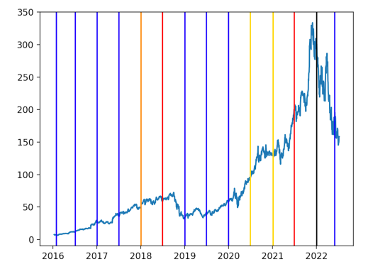
Figure 1: Nvidia Corporation stock prices (USD). The lines illustrate the dates considered to detect a bubble with our methodology. The colors change based on the probability $P_{b}$ that the asset has a bubble according to our methodology. In particular: for the red lines we have $P_{b}>95\%$, for the orange line $P_{b}=85\%$, for the gold lines $70\%<P_{b}<73\%$, for the black line $P_{b}=48\%$ and for the blue lines $P_{b}<2\%$.

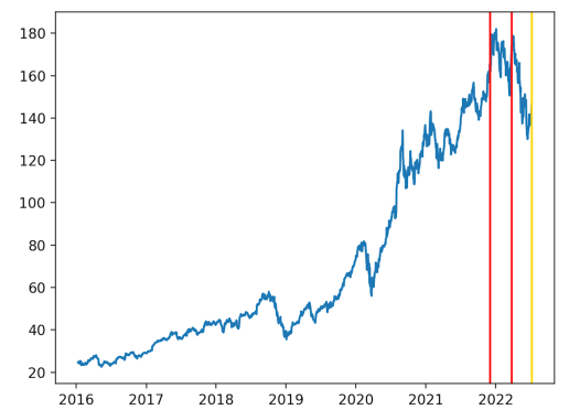
Figure 2: Apple Inc. stock prices (USD). The lines illustrate the dates considered to detect a bubble with our methodology. The colors change based on the probability $P_{b}$ that the asset has a bubble according to our methodology. In particular, for the red lines we have $P_{b}>95\%$ and for the gold one $P_{b}=71.8\%$.

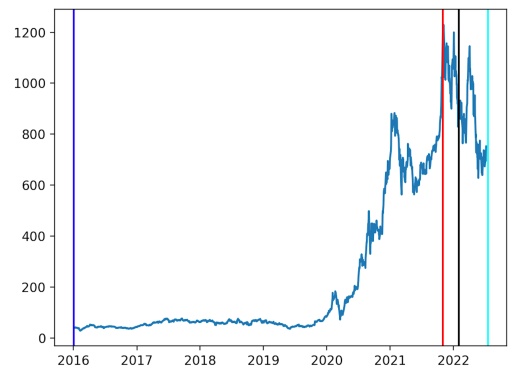
Figure 3: Tesla Inc. stock prices (USD). The lines illustrate the dates considered to detect a bubble with our methodology. The colors change based on the probability $P_{b}$ that the asset has a bubble according to our methodology. In particular: for the red line we have $P_{b}=99.8\%$, for the black line $P_{b}=49.5\%$, for the cyan line $P_{b}=38\%$ and for the blue one $P_{b}=0.1\%$

4.0.2 Apple Inc.

The second objective of our analysis on real data is Apple, whose price increased more than twofold from early 2020 to late 2021. This very steep increase might indicate an over-valuation of Apple’s stock price, above the fundamental value. However, it is of course hard to assess if the stock price of such a huge and successful company is actually over-valued, and we use our methodology to give a partial answer.

We consider three dates: 1st of December 2021, 24th of March 2022 and 8th of July 2022. As can be observed in Figure 2, the first date is before and the second two after the peak of Apple price in December 2021. The network attributes a probability $P_{b}$ that the asset has a bubble equal to $95.3\%$ and $90.5\%$ the first two dates, respectively, and $P_{b}=71.8\%$ in July 2022.

4.0.3 Tesla Inc.

As a third example, we focus on the case of Tesla. The Tesla stock price has seen an extremely steep increase in last years, of about $30000\%$ from early 2016 to the peak in late 2021. Because of such a huge boost, many experts claimed that the stock is affected by a bubble, see for example Libich et al. (2021). By using our methodology we assess if a bubble is present or not four dates, which are shown in Figure 3. The color of the lines which identify the dates corresponds to the probability $P_{b}$ assigned by our methodology for the presence of a bubble. The algorithm outputs $P_{b}=0.1\%$ the 3rd of January 2016, $P_{b}=99.8\%$ the 1st of November 2021 (right before the peak of the stock price), $P_{b}=49.5\%$ the 1st of February 2022 (right after the peak) and $P_{b}=38\%$ the 17th of July 2022.

5 Conclusion

In this article we propose a deep learning-based methodology to detect financial asset price bubbles, where a deep neural network is trained using synthetic option price data generated from a collection of models. For instance, we use local and stochastic volatility models, in which the presence of a bubble is determined by the value of certain parameters. This trained neural network is then used for bubble detection in more general situations. The deep neural network takes as input call option prices for a given underlying and returns as output a number in $[0,1]$, which indicates the probability that the underlying exhibits a bubble.

We have assessed the performance of the methodology on both synthetic and real data. First we have tested various settings in which the network is trained using a certain class of local or stochastic volatility models and tested within another class. In particular, a high out-of-sample prediction accuracy has been observed when two model classes are used for training and the trained network is used for bubble detection in another class of models. We have also tested the methodology with market data of three tech stocks at various dates and have observed a close match between the output of the network and the (retrospectively) expected results. Furthermore, these numerical experiments have been complemented by a mathematical proof for the method in a local volatility setting. Extensions of these theoretical results to more general model classes are also possible, provided an analogue of the “bubble detection function” $F$ can be constructed. On the other hand, the proposed algorithm could be directly modified to take into account additional market factors as inputs for the neural network, provided that these factors can be incorporated into the models used to generate the training data.

References

- Bercovici (2017) Jeff Bercovici. Yes, it’s a Tech Bubble. Inc., 2017. URL https://www.inc.com/magazine/201509/jeff-bercovici/are-we-in-a-tech-bubble.html.
- Biagini et al. (2014) Francesca Biagini, Hans Föllmer, and Sorin Nedelcu. Shifting martingale measures and the slow birth of a bubble. Finance and Stochastics, 18(2):297–326, 2014.
- Cox and Hobson (2005) Alexander MG Cox and David G Hobson. Local martingales, bubbles and option prices. Finance and Stochastics, 9(4):477–492, 2005.
- Dias et al. (2020) José Carlos Dias, João Pedro Vidal Nunes, and Aricson Cruz. A note on options and bubbles under the CEV model: implications for pricing and hedging. Review of Derivatives Research, 23(3):249–272, 2020.
- Ekström and Tysk (2012) Erik Ekström and Johan Tysk. Dupire’s equation for bubbles. International Journal of Theoretical and Applied Finance, 15(06):1250041, 2012.
- Fusari et al. (2020) Nicola Fusari, Robert A. Jarrow, and Sujan Lamichhane. Testing for asset price bubbles using options data. Johns Hopkins Carey Business School Research Paper, (20-12), 2020.
- Heston et al. (2007) Steven L Heston, Mark Loewenstein, and Gregory A Willard. Options and bubbles. The Review of Financial Studies, 20(2):359–390, 2007.
- Hornik (1991) Kurt Hornik. Approximation capabilities of multilayer feedforward networks. Neural Networks, 4(1989):251–257, 1991.
- Jacquier and Keller-Ressel (2018) Antoine Jacquier and Martin Keller-Ressel. Implied volatility in strict local martingale models. SIAM Journal on Financial Mathematics, 9(1):171–189, 2018.
- Jarrow (2016) Robert A. Jarrow. Testing for asset price bubbles: three new approaches. Quantitative Finance Letters, 4(1):4–9, 2016.
- Jarrow and Kwok (2021) Robert A. Jarrow and Simon S. Kwok. Inferring financial bubbles from option data. Journal of Applied Econometrics, 36(7):1013–1046, 2021.
- Jarrow et al. (2007) Robert A. Jarrow, Philip Protter, and Kazuhiro Shimbo. Asset price bubbles in complete markets. Advances in Mathematical Finance, In Honor of Dilip B. Madan:105–130, 2007.
- Jarrow et al. (2010) Robert A. Jarrow, Philip Protter, and Kazuhiro Shimbo. Asset price bubbles in incomplete markets. Mathematical Finance, 20(2):145–185, 2010.
- Jarrow et al. (2011a) Robert A. Jarrow, Younes Kchia, and Philip Protter. How to detect an asset bubble. SIAM Journal on Financial Mathematics, 2(1):839–865, 2011a.
- Jarrow et al. (2011b) Robert A. Jarrow, Younes Kchia, and Philip Protter. Is there a bubble in Linkedin’s stock price? The Journal of Portfolio Management, 38(1):125–130, 2011b.
- Kolakowski (2019) Mark Kolakowski. Nvidia’s stock signals techs near bubble like 2000. 2019. URL https://www.investopedia.com/news/nvidia/l.
- Libich et al. (2021) Jan Libich, Liam Lenten, et al. Bitcoin, Tesla and GameStop bubbles as a flight to focal points. World Economics, 22(1):83–108, 2021.
- Lindsay and Brecher (2012) Alan E Lindsay and DR Brecher. Simulation of the CEV process and the local martingale property. Mathematics and Computers in Simulation, 82(5):868–878, 2012.
- Loewenstein and Willard (2000) Mark Loewenstein and Gregory A. Willard. Rational equilibrium asset-pricing bubbles in continuous trading models. Journal of Economic Theory, 91(1):17–58, 2000.
- Ozimek (2017) Adam Ozimek. There obviosly is a tech bubble, but hopefully that doesn’t matter. Forbes, 2017. URL https://www.forbes.com/sites/modeledbehavior/2017/07/16/there-obviously-is-a-tech-bubble-but-hopefully-that-doesnt-matter/#737270d9d426.
- Piiroinen et al. (2018) Petteri Piiroinen, Lassi Roininen, Tobias Schoden, and Martin Simon. Asset price bubbles: An option-based indicator. arXiv preprint arXiv:1805.07403, 2018.
- Protter (2013) Philip Protter. A mathematical theory of financial bubbles, volume 2081 of Lecture Notes in Mathematics of V. Henderson and R. Sincar editors, Paris-Princeton Lectures on Mathematical Finance. Springer, 2013.
- Revuz and Yor (2013) Daniel Revuz and Marc Yor. Continuous martingales and Brownian motion, volume 293. Springer Science & Business Media, 2013.
- Serla (2017) Rusli Serla. The tech bubble: how close is it to bursting? Telegraph, 2017. URL http://www.telegraph.co.uk/technology/2017/06/22/tech-bubble-close-bursting/.
- Sharma (2017) Ruchir Sharma. When will the tech bubble burst? New York Times, 2017. URL https://www.nytimes.com/2017/08/05/opinion/sunday/when-will-the-tech-bubble-burst.html.
- Sin (1998) Carlos A. Sin. Complications with stochastic volatility models. Advances in Applied Probability, 30(1):256–268, 1998.