Autoionizing Polaritons with the Jaynes-Cummings Model

Abstract

Intense laser pulses have the capability to couple resonances in the continuum, leading to the formation of a split pair of autoionizing polaritons. These polaritons can exhibit extended lifetimes due to interference between radiative and Auger decay channels. In this work, we introduce an extension of the Jaynes-Cummings model to autoionizing states. This model quantitatively reproduces the observed phenomenology and it allows us to study how the dressing laser parameters can be tuned to control the ionization rate of the polariton multiplet. We illustrate the potential of this model by estimating the splitting and widths of the polaritonic features in the attosecond transient-absorption spectrum of the argon atom in the energy region close to the $3s^{-1}n\ell$ autoionizing states. The model’s predictions are compared with ab initio simulations of the spectrum under realistic experimental conditions.

I Introduction

Attosecond pump-probe spectroscopy has gained prominence as a useful tool for probing and controlling ultrafast electronic dynamics in atoms Berrah et al. (1996); Lukin and Imamoğlu (2001); Fleischhauer et al. (2005); Pazourek et al. (2015); Goulielmakis et al. (2010); Månsson et al. (2014); Jiménez-Galán et al. (2014); Argenti et al. (2015); Kotur et al. (2016); Lin and Chu (2013); Ossiander et al. (2016); Chu and Lin (2010); Douguet et al. (2016); Barreau et al. (2016), molecules Xie et al. (2012); Joffre (2007); Peng et al. (2015); Wang et al. (2021); Asenjo-Garcia et al. (2017); Haessler et al. (2010); Lépine et al. (2014); Huppert et al. (2016), and condensed matter Sidiropoulos et al. (2022); Krüger et al. (2011); Fan et al. (2022). In the electronic continuum of polyelectronic atoms and molecules, there exist localized transiently bound states prone to Auger decay. These states, which are essential for the control of photoelectron emission processes Lindroth and Argenti (2012), appear as asymmetric peaks in the photo-absorption profile of atoms and molecules, due to interference between the direct-ionization path, and the radiative excitation to the metastable state followed by its autoionization Fano and Cooper (1965). Quantum coherence, therefore, is an essential feature of these states, which manifests itself also in the temporal evolution of the electronic wavefunction, when interrogated with time resolved spectroscopies Gruson et al. (2016). External fields can modify the evolution of these metastable states, altering their spectral lineshapes and lifetimes Ott et al. (2013). The absorption line of bound or metastable states, when influenced by a dressing laser, varies with laser intensity and the proximity of other resonances. This variation include phenomena such as AC Stark shift Chini et al. (2012), subcycle oscillations of the absorption intensity Chini et al. (2013), modification of the lineshape asymmetry Yang et al. (2015), and Autler-Townes (AT) splitting Ott et al. (2014); Zhao et al. (2017). AT splitting, in particular, has been observed in the absorption profile of atoms both above Wang et al. (2010); Pfeiffer and Leone (2012); Kobayashi et al. (2017); Mihelič et al. (2017) and below Gaarde et al. (2011); Wu et al. (2013); Zhao et al. (2017) the ionization threshold. In 1963, Jaynes and Cumming formulated a model for the AT splitting of two bound states in terms of quantized radiation states Jaynes and Cummings (1963). In this model, the two branches of an AT multiplet are regarded as entangled states of atomic and light configurations, known as polaritons Galego et al. (2015); Zhang et al. (2019); Herrera and Owrutsky (2020).

Recent attosecond transient absorption measurements, corroborated by theoretical calculations, have revealed AT splitting of the $3s^{-1}4p$ resonance in argon, arising from the strong coupling with the $3s^{-1}3d$ dark state Harkema et al. (2021). Given that these states are subject to autoionization decay, we refer to the AT branches as autoionizing polaritons (AIPs).

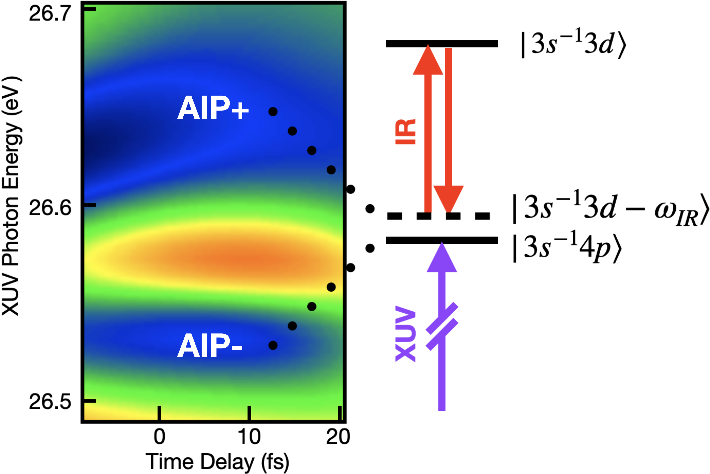
Figure 1: Example of an ab initio transient absorption spectrum in argon. Here, a moderately intense dressing pulse couples the $3s^{-1}4p$ and $3s^{-1}3d$ autoionizing states. The strong IR coupling splits the resonance into a pair of AIPs, which are a linear combinations of the $3s^{-1}4p$ resonance and the $3s^{-1}3d-\omega_{IR}$ light-induced state.

Figure 1 exemplifies this splitting in the simulated extreme ultraviolet (XUV) attosecond transient absorption spectrum of the argon atom. Autoionizing states (AIS), which are immersed in the continuum, are susceptible to photoionization even by low-energy photons like those from the infrared (IR) dressing field. External radiation fields, therefore, may be expected to reduce the lifetime of these states. Contrary to expectations, Lambropolous and Zöller in 1982 posited that the Auger decay amplitude and the photoionization amplitude of a laser-dressed autoionizing state might interfere destructively, thereby stabilizing the state (see last paragraph in Sec. VI of Kim and Lambropoulos (1982)).

In the absence of significant quantum interference, one would expect the AIPs resulting from the coupling of bright and dark states in resonance to have identical widths. However, experimental findings in Harkema et al. (2021) provides evidence that the width of the two polaritons can differ, with one polariton becoming narrower than the original bright state, which demonstrates that coherent stabilization is an observable phenomenon. The enhancement or suppression of the AIP decay rate can be controlled via the laser parameters. Autoionizing polaritons, therefore, differ qualitatively both from bound-state polaritons, which do not have access to Auger decay channels, and from overlapping autoionizing states, in which radiation does not play any role.

In this study, we extend the Jaynes-Cummings (JC) formalism to include autoionization, using Fano’s approach, under certain simplifying assumptions. Our model is capable of describing the optical excitation, from an initial ground state $|g\rangle$, of a pair of autoionizing states, $|a\rangle$ and $|b\rangle$, coupled to each other by an external infrared driving field, and their subsequent decay to the continuum. It quantifies the interference between radiative and nonradiative decay pathways, illustrating how a laser can stabilize an autoionizing state. This framework provides a stepping stone for understanding coherent control of polaritonic states in matter, a key aspect of emerging technologies in quantum sensing Peng et al. (2020), photon trapping, and quantum information processing Song et al. (2016).

This paper is organized as follows. Section II details a simplified version of the extended JC model applicable when the direct ionization amplitude from the ground state to the continuum is negligible and interaction with other autoionizing states is minimal. This section illustrates the idea of the JC model and makes it easier to understand some important features that are observed in the more elaborate model. Section III addresses more general cases involving multiple laser-coupled autoionizing states and the direct ionization from the ground state to the continuum. This latter formalism is appropriate to describe the interference between overlapping polaritons, while also reproducing the Fano-like profiles of isolated resonances. In Section IV, we describe ab initio many-body calculations of argon’s resonant attosecond transient-absorption using the NewStock suite Carette et al. (2013); Harkema et al. (2021), demonstrating converged results with a limited essential-state space. Finally, Section V presents our conclusions.

II Model for radiatively coupled autoionizing states

In this section, we derive the expression for the energy and width of two autoionizing states coupled by a moderately intense dressing infrared laser, under the premise that the resultant polaritons are isolated. These states produce a distinctive optical signature in the XUV absorption cross section of the dressed system, from the ground state. We assume that the ground state remains largely unaffected by the dressing field. For the sake of simplicity, we also assume that direct ionization from the ground state to the continuum is negligible, leading to the appearance of the two dressed autoionizing states as isolated Lorentzian peaks. A more general case is considered in Sec. III

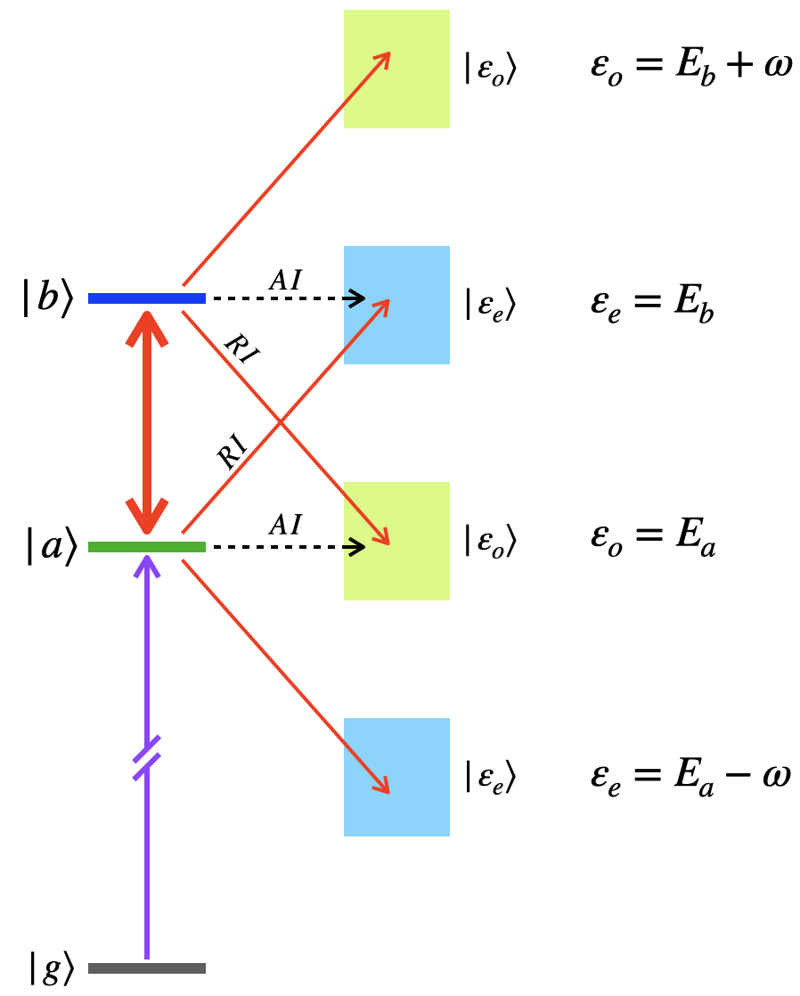
Figure 2: Diagram depicting the various radiative and nonradiative couplings in our model system, which includes a ground state, two AIS of opposite parity, and their respective continua. The radiative coupling from the AIS to the continuum, as well as between the ground and the bright AIS, is treated perturbatively, while the coupling between the localized component of the field-free autoionizing resonances that form the autoionizing polaritons is treated nonperturbatively.

Let’s consider a reference Hamiltonian $H_{0}$ featuring three localized eigenstates: the ground state, $H_{0}|g\rangle=|g\rangle E_{g}$, assumed to have even parity; and two autoionizing states, $H_{0}|a\rangle=|a\rangle E_{a}$ and $H_{0}|b\rangle=|b\rangle E_{b}$, with odd and even parity, respectively. Additionally, $H_{0}$ has two sets of continuum eigenstates, $H_{0}|\varepsilon_{e}\rangle=|\varepsilon_{e}\rangle\varepsilon_{e}$ with even parity, and $H_{0}|\varepsilon_{o}\rangle=|\varepsilon_{o}\rangle\varepsilon_{o}$ with odd parity, for every energy above the threshold $E_{\mathrm{th}}$, $\varepsilon_{e/o}>E_{\mathrm{th}}$. Both autoionizing states are above this threshold, $E_{a},\,E_{b}>E_{\mathrm{th}}$. The complete field-free Hamiltonian, $H=H_{0}+V$, includes the interaction $V$ between bound and continuum configurations, responsible for the Auger decay of the states $|a\rangle$ and $|b\rangle$. In this work, for specificity, we assign the energies of states $g$, $a$, and $b$ to match those of the ground state and the $3s^{-1}4p$ and $3s^{-1}3d$ states of argon Harkema et al. (2021); Yanez-Pagans et al. (2022). Figure 2 schematically representat these energy levels and their radiative couplings.

As an initial approximation, the Auger decay rates can be computed using Fermi’s golden rule Sakurai (1994)

$$\Gamma_{a}=2\pi\left|\langle{\varepsilon}_{o}|V|a\rangle\right|^{2},\quad\Gamma_{b}=2\pi\left|\langle{\varepsilon}_{e}|V|b\rangle\right|^{2}.$$ (1)

To better highlight the effect of stabilization, we intentionally assign identical Auger decay rates and radiative coupling strengths to the continuum for both autoionizing states. In the absence of dressing radiation, the XUV spectrum of the system exhibits a single bright resonance near the energy $E_{a}$ with a width of $\Gamma_{a}$. Given that the XUV pulse is weak, as hypothesized, the absorption of one XUV photon from the ground state to the continuum is accurately modeled semiclassically, using first-order perturbation theory. Consequently, the optical density is directly proportional to the square modulus of the dipole transition amplitude from the ground state to the resonant continuum. In this simplified model, the oscillator strength is derived solely from the radiative coupling of the ground state to the localized component of the autoionizing states. As such, the background contribution from direct ionization to the non-resonant continuum is not present, leading to absorption peaks with Lorentzian profiles.

To describe the strong radiative coupling between states $|a\rangle$ and $|b\rangle$ due to infrared dressing light, a quantized formalism for the radiation is more convenient than the semiclassical approach. For large number of photons and for laser fields described by coherent states, the two approaches are equivalent Cohen-Tannoudji (1996). This formalism also allow us to describe the concurrent transition from either of these two states to the continuum. The vector-potential operator for a single IR radiation mode with frequency $\omega$ and polarization $\hat{\epsilon}$, in a cubic box with edge length $L$ and periodic boundary conditions, is defined as Cohen-Tannoudji et al. (1989)

$$\vec{A}_{\textsc{IR}}=\left(\frac{2\pi c}{L^{3}k}\right)^{1/2}\left(\hat{\epsilon}\,\eta+\hat{\epsilon}^{*}\,\eta^{\dagger}\right),$$ (2)

where $k=\omega/c$, $c$ is the speed of light in vacuum, and $\eta^{\dagger}$ and $\eta$ are the photon creator and annihilation operators, respectively, with $\eta|n\rangle=\sqrt{n}|n-1\rangle$ and $\eta^{\dagger}|n\rangle=\sqrt{n+1}|n+1\rangle$. Gauss units Jackson (1975) and atomic units ($\hbar=1$, $m_{e}=1$, $q_{e}=-1$) are used throughout the paper unless specified otherwise.

The free-radiation Hamiltonian for this mode is $H_{R}=\omega b^{\dagger}b$, neglecting the zero-point energy as it is irrelevant in our context. A photon-state $|n\rangle$ thus has energy $n\omega$, with $H_{R}|n\rangle=n\omega|n\rangle$. The average number of photons per unit volume, $n/L^{3}$, is related to the laser intensity $I$ as $n/L^{3}=I/(\omega c)$. The minimal-coupling radiation-matter interaction Hamiltonian is given by $H_{I}=\alpha\vec{A}_{IR}\cdot\vec{p}$, where $\alpha=1/c$ is the fine-structure constant, $\vec{p}$ is the canonical electron momentum, and we assume the dipole approximation ($\omega r/c\ll 1$).

In this study, we focus on a moderately intense dressing laser of frequency $\omega$ with a small detuning $\delta=E_{b}-E_{a}-\hbar\omega$ from the resonant transition between $|a\rangle$ and $|b\rangle$. Under these conditions, the states $|a\rangle$ and $|b\rangle$ are strongly coupled, while their radiative coupling to the continuum remains weak. Given its large excitation energy, we can further assume that the ground state $|g\rangle$ is not significantly affected by the dressing field. Furthermore, at moderate intensities, where the ponderomotive energy is a negligible fraction of the laser frequency, we can safely disregard the laser dressing of the continuum, including radiative continuum-continuum transitions. Any of these effects, of course, may play a role for sufficiently intense dressing fields or for observables other than the XUV absorption spectrum of the laser-dressed atom in the proximity of $\omega_{\textsc{XUV}}\sim E_{a}-E_{g}$, such as the photoelectron sidebands at energies $\omega_{\textsc{XUV}}\sim E_{a}-E_{g}\pm\omega_{\textsc{IR}}$. For moderately intense IR fields, however, the resonant coupling between autoionizing states and their photoionization by the IR to the continuum are expected to dominate.

To limit the interaction to these processes, we modify the interaction Hamiltonian $H_{I}$ to an ad hoc operator $\bar{H}_{I}$ that deliberately excludes laser dressing of the ground state and the continuum,

$$\begin{split}\bar{H}_{I}&=H_{I}-P_{g}H_{I}-H_{I}P_{g}-QH_{I}Q,\end{split}$$ (3)

where $P_{g}=|g\rangle\langle g|$, and $Q=\int d\varepsilon\left(|\varepsilon_{e}\rangle\langle\varepsilon_{e}|+|\varepsilon_{o}\rangle\langle\varepsilon_{o}|\right)$. The total Hamiltonian for matter and the dressing field, therefore, is expressed as

$$H=H_{0}+V+H_{R}+\bar{H}_{I}.$$ (4)

We assume that the unperturbed bound and continuum states are defined such that the only non-zero residual elements of the configuration-interaction operator $V$ is between an autoionizing state, $|a\rangle$ or $|b\rangle$, and the continuum with the same parity. The Hamiltonian $H$ acts on the Hilbert space for both radiation and matter, represented by the tensor-product space $\mathcal{H}=\mathcal{H}_{el}\otimes\mathcal{H}_{r}$, where $\mathcal{H}_{el}=\mathrm{Span}\{|g\rangle,|a\rangle,|b\rangle,|{\varepsilon}_{e}\rangle,|{\varepsilon}_{o}\rangle\}_{\varepsilon_{e/o}\in[E_{\mathrm{thr}},\infty]}$ and $\mathcal{H}_{R}=\mathrm{Span}\{|n\rangle,\,n\in\mathbb{N}\}$.

It is useful to decompose the Hamiltonian into a component $H_{0}^{\prime}$ that accounts for the radiative transitions between $|a\rangle$ and $|b\rangle$, and a residual part $V^{\prime}$, responsible for the radiative and non-radiative coupling to the continuum, which we will address perturbatively,

$$\begin{split}H&=H_{0}^{\prime}+V^{\prime}\\ H_{0}^{\prime}&=H_{0}+H_{R}+PH_{I}P,\\ V^{\prime}&=V+PH_{I}Q+QH_{I}P,\end{split}$$ (5)

where the projector $P$ is defined as $P=|a\rangle\langle a|+|b\rangle\langle b|$. In this context, the continuum states $|{\varepsilon}_{o/e},n\rangle=|{\varepsilon}_{o/e}\rangle\otimes|n\rangle$, are already eigenstates of $H_{0}^{\prime}$. The other eigenstates are linear combinations of the states $|a,n\rangle\equiv|a\rangle\otimes|n\rangle$ and $|b,n^{\prime}\rangle$, which are entangled states of matter and radiation, commonly known as polaritons Fox (2001). To further simplify, we assume that only configurations of the form $|a,n\rangle$ and $|b,n-1\rangle$ significantly mix, effectively leading us to the well-known Jaynes-Cummings model Jaynes and Cummings (1963). This assumption is equivalent to the rotating-wave approximation in the semi-classical description of the Rabi oscillations Rabi (1937).

The eigenstates of $H_{0}^{\prime}$ are obtained by diagonalizing the Hamiltonian in the $2\times 2$ basis of $|a,n\rangle$ and $|b,n-1\rangle$,

$$\begin{split}\langle a,n|H|a,n\rangle&=E_{a}+n\omega\\ \langle b,n-1|H|b,n-1\rangle&=E_{b}+(n-1)\omega\phantom{\sqrt{\frac{2\pi}{c}}}\\ \langle a,n|H|b,n-1\rangle&=\sqrt{\frac{2\pi}{c}}\,\frac{I^{1/2}}{\omega}p_{ab},\end{split}$$ (6)

where $p_{ab}=\langle a|\hat{\epsilon}\cdot\vec{p}|b\rangle$. When the IR dressing field frequency is in resonance with the radiative transition between $|a\rangle$ and $|b\rangle$, $|a\rangle$ and the light-induced state from $|b\rangle$ become degenerate, leading to the formation of a pair of autoionizing polaritons. These two polaritonic solutions,

$$|\Psi^{\pm}\rangle=|a,n\rangle\,C_{a}^{\pm}+|b,n-1\rangle\,C_{b}^{\pm},$$ (7)

with eigenvalues $E_{\pm}=E_{a}+n\omega+\varepsilon_{\pm}$, satisfy the following secular equation,

$$\left(\begin{array}[]{cc}0&\gamma_{ab}\\ \gamma_{ab}^{*}&\delta\end{array}\right)\left(\begin{array}[]{c}C_{a}^{\pm}\\ C_{b}^{\pm}\end{array}\right)=\varepsilon_{\pm}\left(\begin{array}[]{c}C_{a}^{\pm}\\ C_{b}^{\pm}\end{array}\right),$$ (8)

where $\gamma_{ab}=\sqrt{\frac{2\pi I}{\omega^{2}c}}\,p_{ab}$, $\delta=E_{b}-E_{a}-\omega$, and

$$\varepsilon_{\pm}=\frac{\delta}{2}\pm\frac{\Omega}{2},\qquad{\Omega}=\sqrt{\delta^{2}+\Omega_{0}^{2}},\quad\Omega_{0}=2\gamma_{ab}.$$ (9)

Here, ${\Omega}$ is the familiar Rabi frequency. Indeed, $I=E_{0}^{2}c/8\pi$, and hence $\Omega_{0}=|p_{ab}E_{0}/\omega|=|\mu_{ab}E_{0}|$. The corresponding eigenvectors are

$$\begin{split}|\Psi^{+}\rangle&=\phantom{-}\cos\theta\,|a;n\rangle+\sin\theta\,|b;n-1\rangle,\\ |\Psi^{-}\rangle&=-\sin\theta\,|a;n\rangle+\cos\theta\,|b;n-1\rangle,\end{split}$$ (10)

where $\theta=\arctan[\Omega_{0}/(\Omega-\delta)]$. Since this simplified model does not account for non-resonant radiative interaction with the other states of the system, it cannot reproduce the effect of the ac-Stark shift of the states, which is often observed in real systems. The more complex model described in the next section, III, which considers a larger set of interacting resonances, can reproduce this effect, and so can the ab initio models discussed in Section IV. In the present case study, while an asymmetric shift is visible in the data, the effect is minimal compared to the formation of polaritonic features.

Figure 3 illustrates the six different paths to the four final continuum channels. If the two polaritonic states are energetically well separated, we can estimate their decay rates using Fermi’s golden rule,

$$\Gamma^{\pm}=\sum_{\pi,n^{\prime}}\Gamma^{\pm}_{\varepsilon_{\pi},n^{\prime}},\quad\Gamma^{\pm}_{\varepsilon_{\pi},n^{\prime}}=2\pi\left|\langle\varepsilon_{\pi},n^{\prime}|V^{\prime}|\Psi_{\pm}\rangle\right|^{2}.$$ (11)

In this context, the summation is limited to four distinct final channels (See Fig.  3),

$$\begin{split}\Gamma^{\pm}&=\Gamma^{\pm}_{\varepsilon_{e}=E_{b},n-1}+\Gamma^{\pm}_{\varepsilon_{o}=E_{a},n}+\\ &+\Gamma^{\pm}_{\varepsilon_{e}=E_{a}-\omega,n+1}+\Gamma^{\pm}_{\varepsilon_{o}=E_{b}+\omega,n-2}.\end{split}$$ (12)

Two of these decay channels, $|\Psi^{\pm}\rangle\to|\varepsilon_{o}=E_{a}-\omega,n+1\rangle$ and $|\Psi^{\pm}\rangle\to|\varepsilon_{e}=E_{b}+\omega,n-2\rangle$, result from individual quantum paths involving either the coherent emission or absorption of a photon. Since these paths do not interfere with any others, their decay rates contribute incoherently to the total rate.

Conversely, in the remaining two channels, Auger decay from each polaritonic component ($|a,n\rangle$ or $|b,n-1\rangle$) interferes with a radiative ionization path from the other component, thus enhancing or suppressing the overall decay rate.

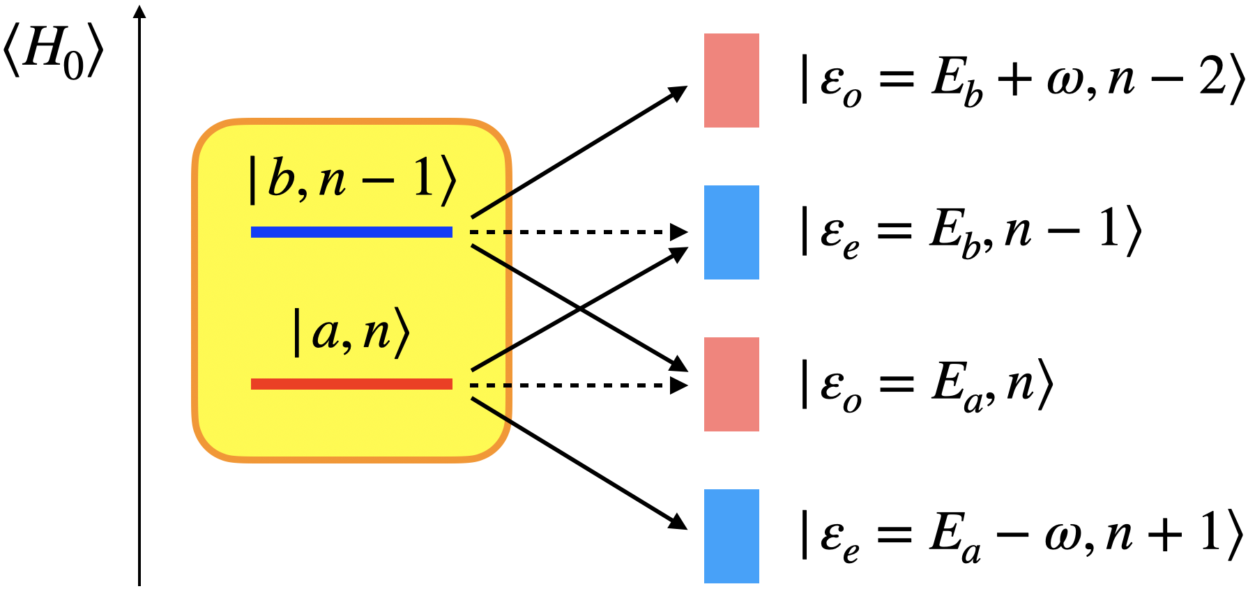
Figure 3: Decay paths of one autoionizing polariton (yellow box on the left). The vertical axis represents the expectation value of the non-interacting electronic Hamiltonian. The energies of the two components of the polariton are shown separately for clarity. The four possible final continuum channels to which the polariton decays are shown on the right. Dashed arrows represent Auger decay, where the number of photons does not change, while continuum arrows represent either the stimulated emission or absorption of one photon that accompanies the ionization of a polaritonic component, for a total of six transition paths. For each of the two central final continuum channels, two distinct paths interfere: Auger decay of one component and the photoionization (in either absorption or emission) of the other component, leading the same final energy and parity in the continuum.

The partial decay rates for the two channels where autoionization and radiative ionization interfere are expressed as follows:

$$\Gamma^{\pm}_{\varepsilon_{e}=E_{b},n-1}=2\pi\left|\,\frac{1}{\omega}\,\sqrt{\frac{2\pi I}{c}}\,p_{\varepsilon_{e}a}\,C_{a}^{\pm}+V_{\varepsilon_{e},b}\,C_{b}^{\pm}\,\right|^{2}$$ (13)

where we have used the relation

$$\langle\varepsilon_{e},n-1|V^{\prime}|a,n\rangle=\frac{1}{\omega}\sqrt{\frac{2\pi I}{c}}\,p_{\varepsilon_{e}a}.$$ (14)

Recognizing that $\Gamma_{AI,b}=2\pi|V_{\varepsilon_{e},b}|^{2}$ is the Auger width of the $|b\rangle$ state and introducing $\Gamma_{PI,a}=4\pi^{2}Ip^{2}_{E_{\beta},a}/\omega^{2}$ as the decay rate associated to the photoionization of $|a\rangle$, the width $\Gamma_{\varepsilon_{e}=E_{b},n-1}^{\pm}$ can be reformulated as

$$\begin{split}\Gamma^{\pm}_{\varepsilon_{e}=E_{b},n-1}&=\left|\,\Gamma^{1/2}_{PI,a}\,C_{a}^{\pm}+\Gamma^{1/2}_{AI,b}\,C_{b}^{\pm}\,\right|^{2}=\\ &=\Gamma_{PI,a}\left|C_{a}^{\pm}\right|^{2}+\Gamma_{AI,b}\left|C_{b}^{\pm}\right|^{2}+\\ &+2\,\Gamma^{1/2}_{PI,a}\,\Gamma^{1/2}_{AI,b}\,\,\real\left({C_{a}^{\pm}}^{*}\,C_{b}^{\pm}\right).\end{split}$$ (15)

Similarly, for the other channel with interference:

$$\Gamma^{\pm}_{\varepsilon_{o}=E_{a},n}=\left|\Gamma^{1/2}_{AI,a}\,C_{a}^{\pm}+\Gamma^{1/2}_{PI,b}\,C_{b}^{\pm}\right|^{2}.$$ (16)

As mentioned earlier, the two remaining channels do not exhibit interference,

$$\begin{split}\Gamma^{\pm}_{b,E_{\alpha}-\omega,n+1}&=\Gamma_{PI,a}\left|C_{a}^{\pm}\right|^{2},\\ \Gamma^{\pm}_{a,E_{\beta}+\omega,n-2}&=\Gamma_{PI,b}\left|C_{b}^{\pm}\right|^{2}.\end{split}$$ (17)

The total ionization rate is thus given by

$$\begin{split}\Gamma^{\pm}=&\,(2\Gamma_{PI,a}+\Gamma_{AI,a})\left|C_{a}^{\pm}\right|^{2}+\\ +&\,(2\Gamma_{PI,b}+\,\Gamma_{AI,b})\left|C_{b}^{\pm}\right|^{2}+\\ +&\,2\,(\Gamma^{1/2}_{PI,a}\Gamma^{1/2}_{AI,b}+\Gamma^{1/2}_{AI,a}\Gamma^{1/2}_{PI,b})\,\,\,\real\left({C_{a}^{\pm}}^{*}C_{b}^{\pm}\right).\end{split}$$ (18)

Depending on the detuning $\delta$ and laser intensity $I$, the interference term can either enhance or suppress the decay rate to the channel. This is the mechanism with which one of the two polaritonic branches can be stabilized. Notice that, at sufficiently low laser intensities, the interference term becomes dominant over the quadratic photoionization term.

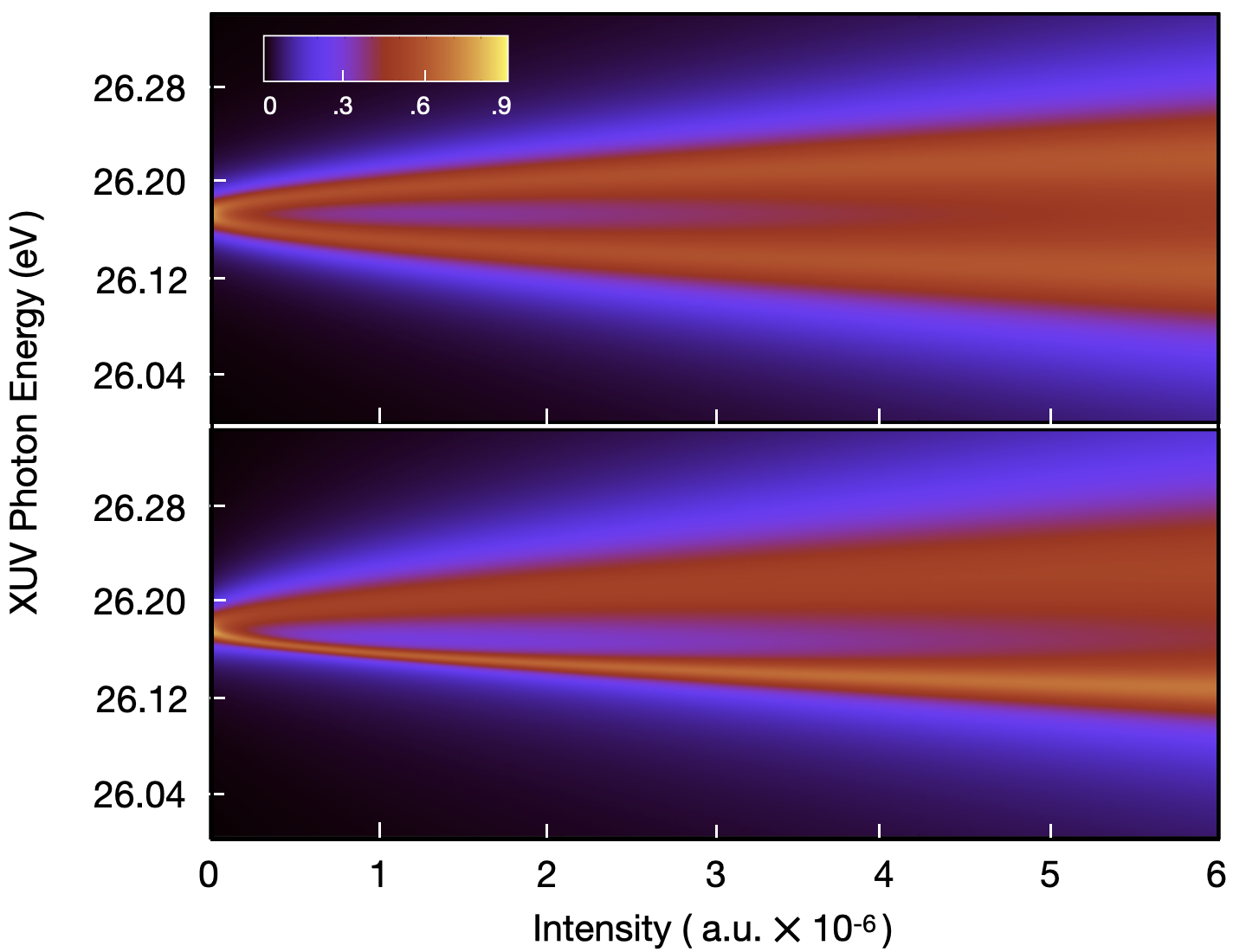
Figure 4: Simulated absorption spectrum (in arbitrary units) as a function of the dressing laser intensity. This model neglects the radiative ionization of the ground state directly to the continuum, therefore the AIPs appear as a pair of Lorentzian functions centered at $\varepsilon_{\pm}$, taken from (9), and have widths $\Gamma^{\pm}$ given by (18). In the upper plot equation (18) has been modified such that the AI and PI terms summed incoherently.

Figure 4 shows a simulated absorption spectrum $\sigma(E;I)$, as a function of the laser intensity. The spectrum is computed using the following equation:

$$\begin{split}\sigma(E;I)=\frac{|p_{ag}|^{2}}{2\pi}\Bigg{[}&\,\,\frac{|C_{a}^{+}|^{2}\,\Gamma^{+}}{(E-E_{+})^{2}+(\Gamma^{+}/2)^{2}}\,\,+\\ +&\,\,\frac{|C_{a}^{-}|^{2}\,\Gamma^{-}}{(E-E_{-})^{2}+(\Gamma^{-}/2)^{2}}\,\,\Bigg{]},\end{split}$$ (19)

where $p_{ag}=\langle a|p|g\rangle$. This model assumes equal Auger widths for states $|a\rangle$ and $|b\rangle$ and neglects direct ionization from the ground to the continuum, leading to Lorentzian profiles for the AIP branches. At higher laser intensities, the two polaritonic branches become clearly distinguishable. The upper plot excludes the interference term from equation (18), causing the radiative and nonradiative terms to sum incoherently, resulting in equal spectral widths for the upper and lower AIP branches. In contrast, the lower plot includes the interference term, making the upper polaritonic branch visibly broader than the lower branch. This demonstrates that the modulation of the polaritonic branches’ widths is due to interference between competing ionization pathways. As equation (18) suggests, for critical values of the detuning and laser intensity, the width of one of the AIP branches can be minimized, thus stabilizing one of the AIP against ionization. This phenomenon is illustrated in Figure 5, where we plot the width of the lower and upper AIP as a function of laser frequency and intensity. The width of the lower branch reaches a minimum when the undressed states $|a\rangle$ and $|b\rangle$ are in resonance and the laser intensity is close to the point of achieving the destructive-interference condition in Eq. (15).

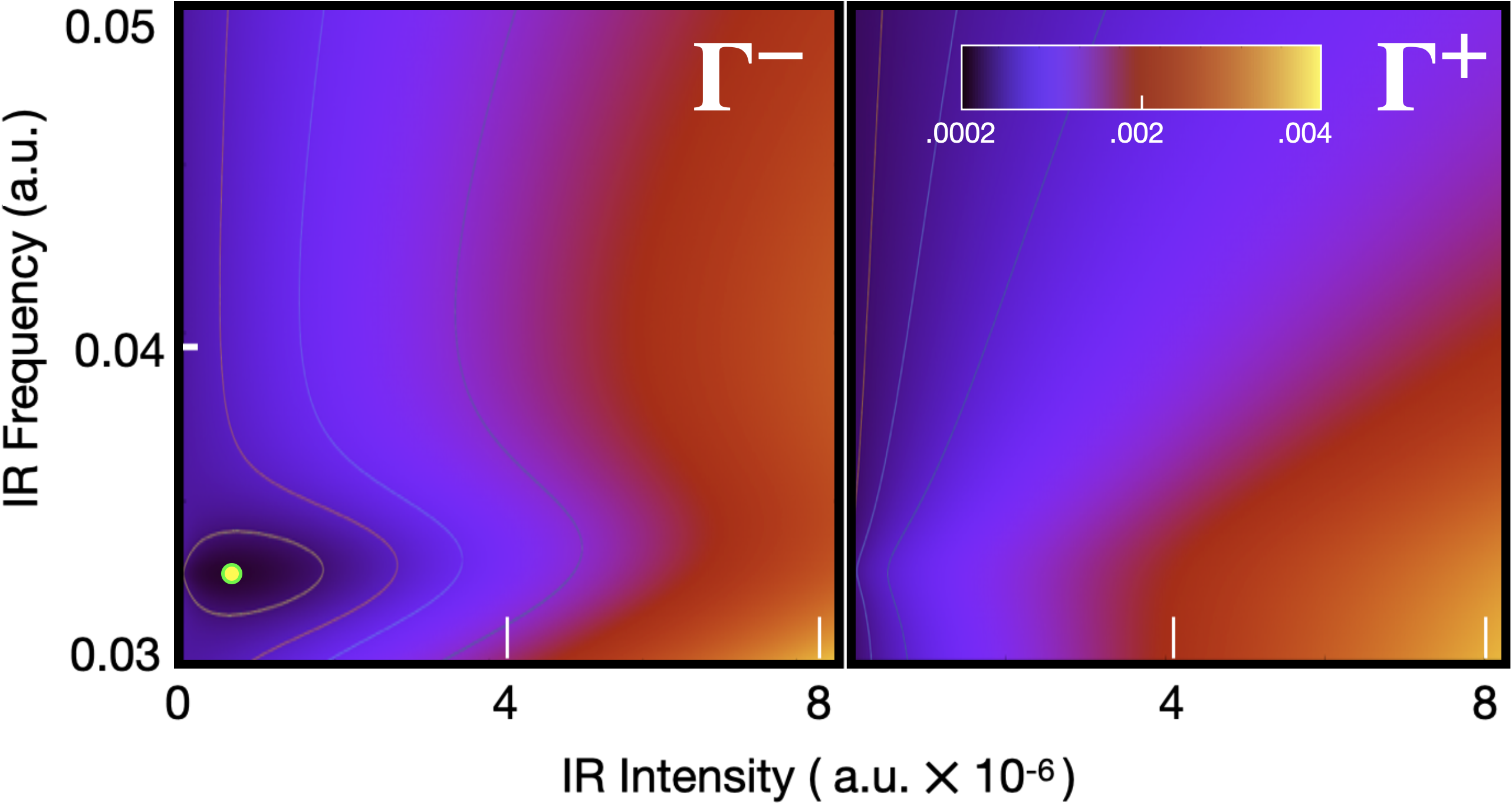
Figure 5: Width of the lower (a) and upper (b) AIP branch as a function of laser detuning and intensity. In the lower branch, a minimum in the width occurs around $\delta=0$, at a critical laser intensity value of $7\times 10^{-6}\,$a.u. (yellow circle).

III Model including direct continuum transitions and Overlapping AIPs

In this section, we expand our model by considering the interference between direct photoionization and resonant-ionization amplitudes. This extension enables our model to reproduce Fano-like profiles of isolated resonances, as well as the more complex interference profile of two overlapping polaritons. This extension, in particular, is essential to reproduce window resonances and the accurate spectral profile of the two polaritons as the laser intensity increases.

As in the previous section, we start with the partitioning of the Hamiltonian in (5). We assume that the ionization of the laser-dressed target can be described in terms of a finite number of localized matter-radiation states, $(|a;n\rangle,|b;n-1\rangle,...)$, which give rise to autoionizing resonances upon interaction with the continuum. Additionally, we consider a finite number of electronic-continuum channels $|\bm{\varepsilon}\rangle=(|\alpha\varepsilon\rangle,|\beta\varepsilon\rangle,...)$, where $\varepsilon$ represents the total energy (photoelectron energy plus radiation field energy) and the channel labels $\alpha$ include discrete quantum numbers identifying the state of the ion, the photoelectron’s angular distribution, their angular and spin coupling, as well as the number of photons in the dressing radiation.

As in the previous section, we assume that the ground state $|g\rangle$ is not coupled by the dressing field to either the localized or the continuum states. Therefore, the initial state can be represented as $|g,n\rangle=|g\rangle\otimes|n\rangle$ for a suitable choice of $n$, presumed to be sufficiently large. We will consider only perturbative transitions from the ground state to the continuum, induced by the absorption of a single XUV photon. The Hamiltonian’s matrix elements within the bound and the continuum sector of the matter states are given by:

$$\langle a,n|H_{0}^{\prime}|a^{\prime},n^{\prime}\rangle=(E_{a}+n\omega)\,\delta_{aa^{\prime}}\delta_{nn^{\prime}}+\sqrt{\frac{2\pi I}{c\omega^{2}}}p_{aa^{\prime}},$$ (20)

$$\langle\alpha\varepsilon|H_{0}^{\prime}|\beta\varepsilon^{\prime}\rangle=\varepsilon\,\delta_{\alpha\beta}\delta(\varepsilon-\varepsilon^{\prime})+\langle\alpha\varepsilon|H_{I}|\beta\varepsilon^{\prime}\rangle.$$ (21)

The interaction between bound and continuum states is:

$$\langle a,n|V+H_{I}|\alpha\varepsilon\rangle=\sqrt{\frac{2\pi I}{c\omega^{2}}}p_{a\varepsilon_{\alpha}}\delta_{|n-n_{\alpha}|,1},$$ (22)

where $\varepsilon_{\alpha}=\varepsilon-n_{\alpha}\omega$.

To determine the eigenstates of the full Hamiltonian, we apply the well-established Fano formalism for multiple bound states interacting with mulltiple continua Fano (1961). Additionally, we introduce a simplifying assumption: for the intensities of the dressing IR laser considered, the continuum-continuum radiative transitions can be neglected. This assumption can be partly mitigated by employing the soft-photon approximation or the similar on-shell approximation Jiménez-Galán et al. (2014),

$$\begin{split}\langle\alpha\varepsilon\|p_{1}\|\beta\varepsilon^{\prime}\rangle&=i\,\delta_{|n_{\alpha}-n_{\beta}|,1}\,\delta(\varepsilon_{\alpha}-\varepsilon_{\beta}^{\prime})\,\delta_{|\ell_{\alpha}-\ell_{\beta}|,1}\,\times\\ &\times\sqrt{2\ell_{>}\varepsilon}\,e^{i(\sigma_{\ell_{\beta}}-\sigma_{\ell_{\alpha}})}.\end{split}$$ (23)

However, for simplicity, we do not pursue this approach here, justified by the fact that, at moderate intensities, the rate of continuum-continuum radiative transitions is negligible compared to the Auger decay rate. Prior to applying Fano’s formalism, it is convenient to diagonalize the bound sector of the Hamiltonian through an orthogonal transformation. We define a set of states $|\Phi_{i}\rangle$ such that

$$|\Phi_{i}\rangle=\sum_{a,n}|a,n\rangle O_{a,n;i}$$ (24)

$$\langle\Phi_{i}|H_{0}^{\prime}|\Phi_{j}\rangle=E_{i}\delta_{ij},\qquad\langle\Phi_{i}|\Phi_{j}\rangle=\delta_{ij}.$$ (25)

Our goal is to find expressions for the stationary wave functions in the continuum, with total energy E, that match prescribed boundary conditions specified by a continuum-channel label $\alpha$. We represent these wave functions as:

$$|\Psi_{\alpha E}\rangle=|\mathbf{\Phi}\rangle\mathbf{f}_{\alpha E}+\ \sum_{\gamma}\int d\varepsilon|\gamma\varepsilon\rangle c_{\gamma\varepsilon,\alpha E},$$ (26)

where $|\mathbf{\Phi}\rangle=(|\Phi_{1}\rangle,\,|\Phi_{2}\rangle,\ldots)$, and $\mathbf{f}_{\alpha E}$ and $c_{\gamma\varepsilon,\alpha E}$ are expansion coefficients. To determine these coefficients, we impose the condition that $|\Psi_{\alpha E}\rangle$ satisfies the secular equation for the total Hamiltonian,

$$(E-H)|\Psi_{\alpha E}\rangle=0.$$ (27)

This equation for the wave function is converted into a system of equations for its expansion coefficients by projecting it on the basis of localized and continuum states. The projection on the bound states reads

$$(E-\mathbf{E})\mathbf{f}_{\alpha E}-\sum_{\gamma}\int d\varepsilon\langle\mathbf{\Phi}|V^{\prime}|\gamma\varepsilon\rangle\,c_{\gamma\varepsilon,\alpha E}=0$$ (28)

where $\mathbf{E}_{ij}=\delta_{ij}E_{i}$, using the relations $\langle\bm{\Phi}|H|\bm{\Phi}\rangle=\bm{E}$, and $\langle\bm{\Phi}|\gamma\varepsilon\rangle=\bm{0}$. The projection on the continua is given by

$$-\langle\beta\varepsilon|V^{\prime}|\mathbf{\Phi}\rangle\mathbf{f}_{\alpha E}+\sum_{\gamma}\int d\varepsilon^{\prime}\langle\beta\varepsilon|E-H|\gamma\varepsilon^{\prime}\rangle\,c_{\gamma\varepsilon^{\prime},\alpha E}=0,$$

which can be reformulated as:

$$(E-\varepsilon)\,c_{\beta\varepsilon,\alpha E}=\langle\beta\varepsilon|V^{\prime}|\mathbf{\Phi}\rangle\mathbf{f}_{\alpha E}.$$ (29)

From Eq. (29), it is possible to express the expansion coefficients on the continuum states in terms of the coefficients of the autoionizing states. The general solution to (29) is given by a particular solution $c^{\prime}_{\beta\varepsilon,\alpha E}$ of that equation, e.g., in principal part,

$$c^{\prime}_{\beta\varepsilon,\alpha E}=\frac{\mathcal{P}\langle\beta\varepsilon|V^{\prime}|\mathbf{\Phi}\rangle\mathbf{f}_{\alpha E}}{E-\varepsilon},$$

plus a solution to the associated homogeneous equation $(E-\varepsilon)\,c^{\mathrm{Hom}}_{\beta\varepsilon,\alpha E}=0$, e.g., $c^{\mathrm{Hom}}_{\beta\varepsilon,\alpha E}=A_{\alpha\beta}\delta(E-\varepsilon)$,

$$c_{\beta\varepsilon,\alpha E}=c^{\prime}_{\beta\varepsilon,\alpha E}+c^{\mathrm{Hom}}_{\beta\varepsilon,\alpha E}.$$ (30)

The choice of matrix $\mathbf{A}$ dictates the boundary conditions and normalization of the solution. Here, we choose $A_{\alpha\beta}=\delta_{\alpha\beta}-i\pi\langle\beta\varepsilon|V^{\prime}|\mathbf{\Phi}\rangle\mathbf{f}_{\alpha E}$, resulting in:

$$c_{\beta\varepsilon,\alpha E}=\delta_{\alpha\beta}\,\delta(\varepsilon-E)\,+\,\frac{\langle\beta\varepsilon|V^{\prime}|\mathbf{\Phi}\rangle\mathbf{f}_{\alpha E}}{E-\varepsilon+i0^{+}}.$$ (31)

This formulation corresponds to a state normalized as $\langle\Psi_{\alpha E}|\Psi_{\beta E^{\prime}}\rangle=\delta_{\alpha\beta}\delta(E-E^{\prime})$ and fulfilling outgoing boundary conditions Newton (1966); Taylor (1972). Replacing this expression in (28), we find an equation for $\mathbf{f}_{\alpha E}$,

$$\mathbf{f}_{\alpha E}=\frac{1}{E-\tilde{\mathbf{H}}(E)}\langle\mathbf{\Phi}|V^{\prime}|\alpha E\rangle.$$ (32)

where we defined the complex effective Hamiltonian $\tilde{\mathbf{H}}(E)$ in the space of localized states as:

$$\tilde{\mathbf{H}}(E)=\mathbf{E}+\sum_{\beta}\int d\varepsilon\frac{\langle\mathbf{\Phi}|V^{\prime}|\beta\varepsilon\rangle\langle\beta\varepsilon|V^{\prime}|\mathbf{\Phi}\rangle}{E-\varepsilon+i0^{+}}.$$ (33)

The term added to the diagonal matrix $\mathbf{E}$ is the sum of the principal part of the integral, and of the residual,

$$\tilde{\mathbf{H}}(E)=\mathbf{E}+\bm{\Delta}(E)-\frac{i}{2}\bm{\Gamma}(E)$$ (34)

where $\bm{\Delta}(E)$ and $\bm{\Gamma}(E)$ are defined as:

$$\bm{\Delta}(E) = \sum_{\beta}\mathchoice{{\vbox{\hbox{$\textstyle-$}}\kern-4.86108pt}}{{\vbox{\hbox{$\scriptstyle-$}}\kern-3.25pt}}{{\vbox{\hbox{$\scriptscriptstyle-$}}\kern-2.29166pt}}{{\vbox{\hbox{$\scriptscriptstyle-$}}\kern-1.875pt}}\!\int d\varepsilon\frac{\langle\mathbf{\Phi}|V^{\prime}|\beta\varepsilon\rangle\langle\beta\varepsilon|V^{\prime}|\mathbf{\Phi}\rangle}{E-\varepsilon},$$ (35)

$$\bm{\Gamma}(E) = 2\pi\sum_{\beta}\langle\mathbf{\Phi}|V^{\prime}|\beta E\rangle\langle\beta E|V^{\prime}|\mathbf{\Phi}\rangle.$$ (36)

To save space, we introduce the vectors $\left[\mathbf{R}_{\alpha E}\right]_{i}=\langle\Phi_{i}|V^{\prime}|\alpha E\rangle$. The expansion coefficients on continuum states are then given by:

$$c_{\beta\varepsilon,\alpha E}=\delta_{\alpha\beta}\delta(\varepsilon-E)\,+\,\frac{\mathbf{R}_{\beta\varepsilon}^{\dagger}[E-\tilde{\mathbf{H}}(E)]^{-1}\,\mathbf{R}_{\alpha E}}{E-\varepsilon+i0^{+}}.$$ (37)

The non-Hermitian effective Hamiltonian $\tilde{\mathbf{H}}(E)$ can be diagonalized, finding a set of left and right eigenvectors,

$$\begin{split}\tilde{\mathbf{H}}(\tilde{E}_{i})\,\mathbf{u}_{R,i}&=\mathbf{u}_{R,i}\,\tilde{E}_{i}\\ \mathbf{u}_{L,i}^{\dagger}\,\tilde{\mathbf{H}}(\tilde{E}_{i})&=\tilde{E}_{i}\,\mathbf{u}_{L,i}^{\dagger}.\end{split}$$ (38)

Assuming that both $\bm{\Delta}(E)$ and $\bm{\Gamma}(E)$ depend only weakly on the parameter $E$, the effective Hamiltonian is essentially the same when evaluated at any of its eigenvalues, $\tilde{\mathbf{H}}(\tilde{E}_{i})\simeq\tilde{\mathbf{H}}(\tilde{E}_{j})$ for any $i$ and $j$. This allows us to drop the energy dependence of the effective Hamiltonian, denoting it simply as $\tilde{\mathbf{H}}$, and solve for all the eigenvectors simultaneously,

$$\tilde{\mathbf{H}}\,\tilde{\mathbf{U}}_{R}=\tilde{\mathbf{U}}_{R}\,\tilde{\mathbf{E}},\qquad\tilde{\mathbf{U}}_{L}^{\dagger}\,\tilde{\mathbf{H}}=\tilde{\mathbf{E}}\,\tilde{\mathbf{U}}_{L}^{\dagger},$$ (39)

where $\tilde{\mathbf{E}}_{ij}=\delta_{ij}\tilde{E}_{i}$ is the diagonal matrix of the complex resonance energies, $\tilde{E}_{i}=\bar{E}_{i}-i\Gamma_{i}/2$, and $\tilde{\mathbf{U}}_{R/L}$ are the matrices of the right and left eigenvectors, respectively, which can now be chosen to be normalized as

$$\tilde{\mathbf{U}}_{L}^{\dagger}\tilde{\mathbf{U}}_{R}=\mathbf{1}.$$ (40)

The expression for $\mathbf{f}_{E}$ then becomes:

$$\mathbf{f}_{\alpha E}=\tilde{\mathbf{U}}_{R}(E-\tilde{\mathbf{E}})^{-1}\tilde{\mathbf{U}}_{L}^{\dagger}\mathbf{R}_{\alpha E}.$$ (41)

Finally, the expansion coefficient on continuum states are

$$\begin{split}c_{\beta\varepsilon,\alpha E}&=\delta_{\alpha,\beta}\,\delta(\varepsilon-E)\,+\\ &+\frac{\mathbf{R}_{\beta\varepsilon}^{\dagger}\tilde{\mathbf{U}}_{R}\,(E-\tilde{\mathbf{E}})^{-1}\,\tilde{\mathbf{U}}_{L}^{\dagger}\mathbf{R}_{\alpha E}}{E-\varepsilon+i0^{+}}.\end{split}$$ (42)

To summarize, we have derived expressions for the expansion coefficients of states in a multi-channel continuum, treating all radiative and non-radiative interactions non-perturbatively, while neglecting continuum-continuum radiative coupling.

In the following, we assume that the energy shift of the resonances due to their interaction with the continuum is negligible compared with the energy gaps between the localized states, $\bm{\Delta}\simeq 0$. The XUV absorption spectrum $\sigma(\omega_{\textsc{xuv}})$ from the laser-dressed system, initially in the ground state with a large number of photons $n\gg 1$, denoted as $|g,n\rangle$, is proportional to the square module of the total dipole transition amplitude, which is given by the incoherent sum of the square module to all the available continuum channels,

$$\sigma(\omega_{\textsc{xuv}})\propto\sum_{\alpha}|\langle g,n|p|\psi_{\alpha E}\rangle|^{2},$$ (43)

where $E=E_{g}+n\omega+\omega_{\textsc{xuv}}$. Using expression (26), the partial photoionization amplitude $\langle g,n|p|\psi_{\alpha E}\rangle$ can be written as

$$\begin{split}\langle g,n|p|\psi_{\alpha E}\rangle&=\langle g,n|p|\mathbf{\Phi}\rangle\mathbf{f}_{\alpha E}+\\ &+\sum_{\beta}\int d\varepsilon\langle g,n|p|\beta\varepsilon\rangle c_{\beta\varepsilon,\alpha E}.\end{split}$$ (44)

Assuming that the radiative coupling with the unperturbed non-resonant continuum is constant in the energy region of interest, $\langle g,n|p|\alpha E\rangle=\delta_{n,n_{\alpha}}p_{g\alpha}$, and using the expressions for the bound and continuum coefficients in 41 and 42, the matrix element between the ground state and the resonant continuum can be expressed as:

$$\langle g,n|p|\psi_{\alpha E}\rangle=p_{g\alpha}+p_{g\alpha}\sum_{j}\frac{\tilde{q}_{j}-i}{\varepsilon_{j}+i},$$ (45)

where $\varepsilon_{j}=2(E-\bar{E}_{j})/\Gamma_{j}$, and the complex asymmetry parameter $\tilde{q}_{j}$ is defined as:

$$\tilde{q}_{j}=\frac{2}{p_{g\alpha}\Gamma_{j}}\left[\left(p_{gn,\bm{\Phi}}+\sum_{\beta}p_{g\beta}\mathchoice{{\vbox{\hbox{$\textstyle-$}}\kern-4.86108pt}}{{\vbox{\hbox{$\scriptstyle-$}}\kern-3.25pt}}{{\vbox{\hbox{$\scriptscriptstyle-$}}\kern-2.29166pt}}{{\vbox{\hbox{$\scriptscriptstyle-$}}\kern-1.875pt}}\!\int\frac{\mathbf{R}_{\beta\varepsilon}^{\dagger}\,d\varepsilon}{E-\varepsilon}\right)\tilde{\mathbf{P}}_{j}\mathbf{R}_{\alpha E}-i\pi\sum_{\beta}\mathbf{R}_{\beta E}^{\dagger}\tilde{\mathbf{P}}_{j}(p_{g\beta}\mathbf{R}_{\alpha E}-p_{g\alpha}\mathbf{R}_{\beta E})\right],$$ (46)

with $\tilde{\mathbf{P}}_{j}=\tilde{\mathbf{U}}_{Rj}\tilde{\mathbf{U}}_{Lj}^{\dagger}$ being the projector on resonance $j$. Notice that the transition amplitude (45) is a coherent sum of the Fano profiles, one for each autoionizing polariton Argenti et al. (2013), generalized to dissipative systems (complex $q$). The interference between the different terms cannot in general be neglected. This expression, therefore, is essential to correctly fit the complex polaritonic multiplets observed in the experiment Harkema et al. (2021).

In the specific case of two AIPs, our system comprises two bound and four continuum components. The bound components, $|\mathbf{\Phi}\rangle=(|\psi_{1}\rangle,|\psi_{2}\rangle)$ (where we use indices $1$ and $2$ for convenience instead of $+$ and $-$), are expressed in terms of $|a\rangle$ and $|b\rangle$ by Eq. (10). The energies of these components depend parametrically on the laser intensity $I$ and angular frequency $\omega$, as detailed in (9). The four continua are $|\alpha(E+2\omega),n-2\rangle$, $|\beta(E+\omega),n-1\rangle$, $|\alpha E,n\rangle$, $|\beta(E-2\omega),n+1\rangle)$. Using Eq. (36), we can callculate the elements of the matrix $\mathbf{\Gamma}$, which can be written in general as

$$\mathbf{\Gamma}_{ij}=2\pi\left[A_{ij}+B_{ij}\sin(2\theta+\phi_{ij})\right],$$ (47)

where $A_{ij}$, $B_{ij}$, and $\phi_{ij}$ are real parameters, which can be determined using appropriate trigonometric relations. Using the relationship (34) we can build and diagonalize the matrix $\mathbf{\tilde{H}}=\mathbf{E}-i\mathbf{\Gamma}/2$, where $\mathbf{E}_{ij}=\delta_{ij}E_{i}$,

$$\mathbf{\tilde{E}}=\begin{bmatrix}E_{+}-i\Gamma_{11}/2&-i\Gamma_{12}/2\\ \\ -i\Gamma_{21}/2&E_{-}-i\Gamma_{22}/2\end{bmatrix},$$ (48)

which has eigenvalues

$$E_{\Omega,1/2} = \frac{E_{1}+E_{2}-i\left(\Gamma_{11}+\Gamma_{22}\right)/2}{2}\pm$$

$$\pm \frac{\sqrt{(E_{1}-E_{2}-i\left(\Gamma_{11}-\Gamma_{22}\right)/2)^{2}-\Gamma_{1,2}\Gamma_{2,1}}}{2}.$$

From these results, we can evaluate the XUV photoabsorption amplitude from (45), as a function of laser intensity and frequency.

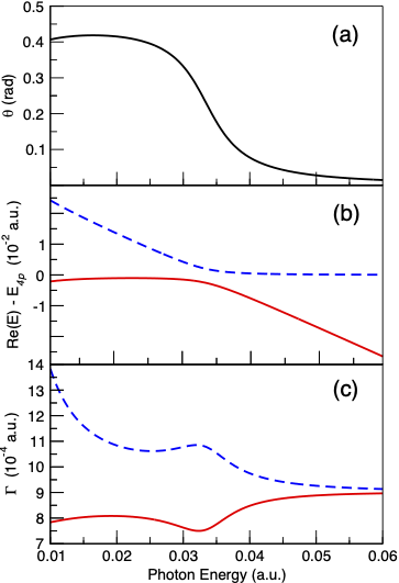
Figure 6: Relevant properties of the autoionizing polaritons, as a function of the dressing-field energy: (a) Mixing angle (see (9)); (b) Real part of the polariton energy with respect to that of the $4p$ bright state; (c) Imaginary part of the polariton energy (i.e., $-\Gamma/2$). See text for details.

Figure 6 shows the mixing angle and the real and imaginary part of the two polariton complex energy, as a function of the laser frequency. The Light-Induced State (LIS) and bright state come in resonance ($\delta=0$) when $\omega=0.033345$ a.u. The polariton energies (Fig. 6b) exhibit a clear avoided crossing associated with a change in character of the polaritonic wavefunction, as shown in the rapid transition of the mixing angle from $~{}90^{\circ}$ to $~{}0^{\circ}$ (Fig. 6a).

Observing the imaginary part of the polaritonic energy in Figure 6c), there is a noticeable dip in the width $\Gamma$ of the lower polariton (red continuous line) at the resonant condition, suggesting its stabilization. Conversely, the width of the upper polariton exhibits a peak at the same frequency, suggesting destabilization. At low frequencies, the width of the upper polariton sharply increases. Although not shown in the figure, the width of the lower polariton also diverges at low frequencies. This behavior is due to the increase in the radiative ionization rate, which is inversely proportional to the laser frequency at constant intensity [see Eq. (22)].

For higher values of the dressing-laser frequency, the LIS and the bright state appear as isolated resonances, with their widths much smaller than their energy separation. Since their lifetime is dominated by the Auger decay rate, which we chose to be identical, their widths converge to the same value.

Figure 7 presents the transient absorption spectrum predicted by the model, as a function of the dressing-laser frequency. This spectrum is calculated assuming a field-free $q$ parameter for the two autoionizing states, which reproduces the window character of the $|3s^{-1}4p,n\rangle$ bright state and of the $|3s^{-1}3d,(n-1)\omega\rangle$ LIS, as observed in the experiment Harkema et al. (2021); Yanez-Pagans et al. (2022). From this spectrum, we can extract both the position and width of the two polaritons, which reproduce those shown in Fig. 6.

When these features are well separated, each exhibits a Fano profile. However, when they overlap, the profile is given by the square of the sum of two Fano-like amplitudes, as detaied in (45), which interfere giving rise to a line shape that cannot be approximated with the sum of two Fano profiles. The absorption spectrum, shown in Figure 7, takes into account both the finite coupling to the non-resonant continuum and the interference effects between closely-spaced branches.

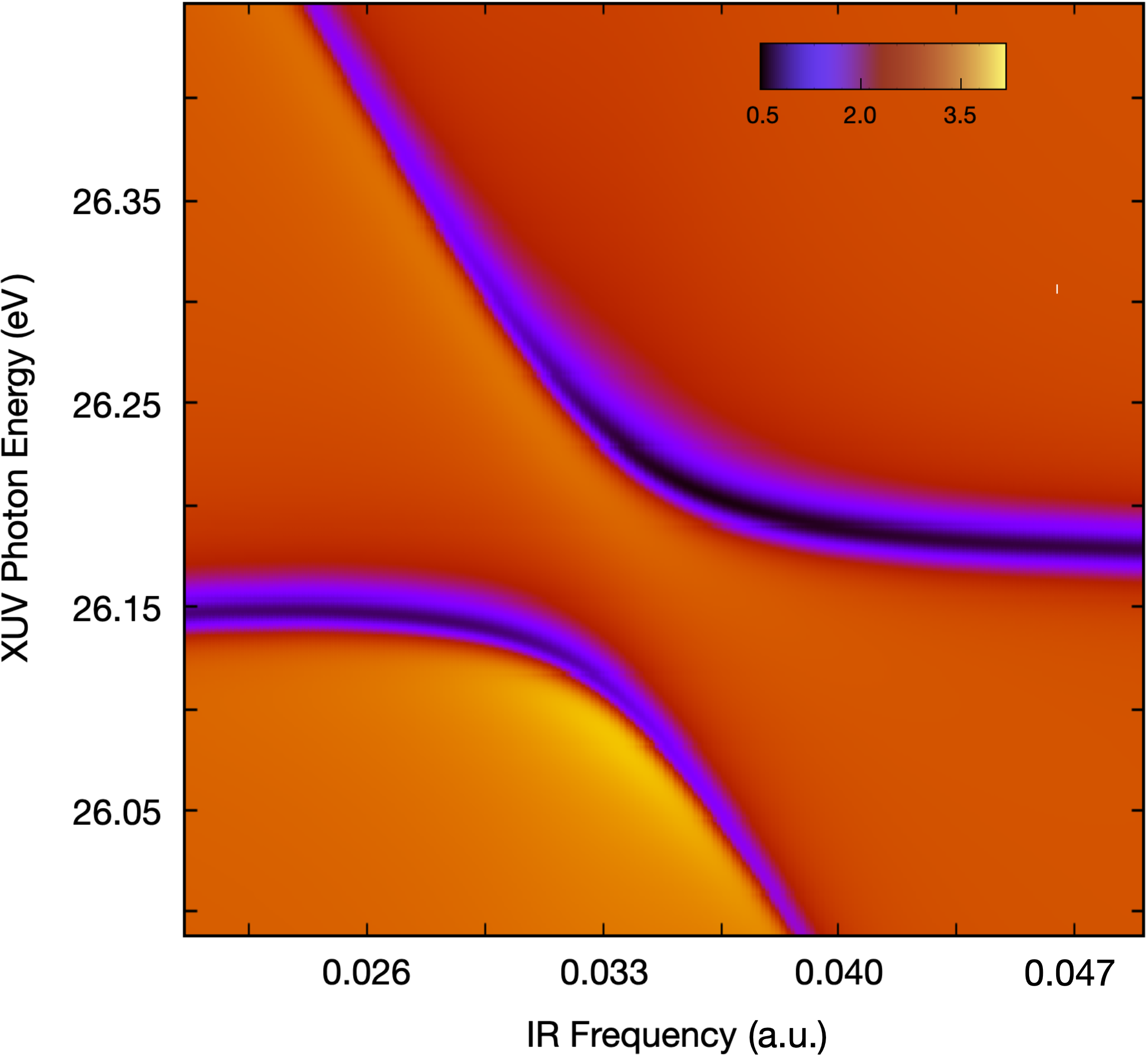
Figure 7: Model-predicted absorption spectrum [in arbitrary units] as a function of IR frequency, based on the formula given in Eq. 43, which accounts for the finite coupling to the non-resonant continuum and the interference between closely-spaced branches.

IV Ab initio calculations

In this section we present ab initio calculations of transient absorption in argon, focusing on the case where the $3s^{-1}4p$ resonance is excited by a weak XUV pump and dressed by a moderately strong IR probe pulse. Depending on its central frequency, the IR pulse may bring in resonance the $3s^{-1}4p$ bright state with other dark or bright resonances by means of one-photon or two-photon transitions, thus causing the resonance peak to split into a pair of AIPs.

For our study, we assume that both the pump and probe pulses are linearly polarized along the same quantization axis. To reproduce the observables measured in a realistic experiment, we compute the transient absorption spectrum both as a function of the pump-probe delay (keeping the IR intensity and frequency constant) and as a function of the IR frequency (at a fixed time delay).

In our ab initio atomic structure calculations, we employ the NewStock suite of atomic codes, developed in LA’s group. For the computation of localized orbitals, we utilize the Multi-configuration Hartree-Fock (MCHF), implemented in the atsp2k atomic-structure package C Froese-Fischer (1997). The orbitals are optimized on the [Ar]$3s^{-1}$ and [Ar]$3p^{-1}$ parent ion configurations. In each symmetry sector $\Gamma=(\Pi,L,S,M,\Sigma)$ -where $\Pi$, $L$, $S$, $M$, and $\Sigma$, are the system’s parity, orbital angular momentum, spin, and their respective projections- we generate the space of configuration-state functions (CSFs), denoted as $|\mathbf{K}^{\Gamma}\rangle$. These CSFs arise from the following shell occupations (for brevity, the inactive neon $1s^{2}2s^{2}2p^{6}$ core is not specified): $3s^{2}3p^{5}$, $3s^{2}3p^{4}3d$, $3s^{2}3p^{4}4s$, $3s^{2}3p^{4}4p$, $3s^{2}3p^{3}3d^{2}$, $3s^{2}3p^{3}3d4s$, $3s^{2}3p^{3}3d4p$, $3s^{2}3p^{3}4s4p$, $3s^{2}3p^{3}4p^{2}$, $3s^{2}3p^{2}3d^{3}$, $3s^{2}3p^{2}3d^{2}4s$, $3s3p^{6}$, $3s3p^{5}3d$, $3s3p^{5}4p$, $3s3p^{4}3d^{2}$, $3s3p^{4}3d4s$, $3s3p^{4}3d4p$, and $3p^{5}3d^{2}$. The shell occupations results in various CSFs, including 25 ${}^{2}S^{e}$ CSFs, 40 ${}^{2}P^{o}$ CSFs, 51 ${}^{2}P^{e}$ CSFs, and 65 ${}^{2}D^{e}$ CSFs. The MCHF procedure also yields a set of optimized ionic states, $\Phi_{a}(x_{1},\ldots,x_{N_{e}-1})$, where $N_{e}=18$ is the number of electrons in the neutral atom, and $x_{i}=(\vec{r}_{i},\zeta_{i})$ is the spatial and spin coordinate of the $i$-th electron,

$$\Phi_{a}(x_{1},\ldots,x_{N_{e}-1})=\sum_{\mathbf{K}}\langle x_{1},\ldots,x_{N_{e}-1}|\mathbf{K}^{\Gamma_{a}}\rangle\,C^{\Gamma_{a}}_{\mathbf{K},a}.$$ (50)

In our atomic calculations, the MCHF ions and orbitals are employed to form a close-coupling basis, which includes a set of partial-wave channels (PWCs), denoted as $\{\phi_{\alpha n}^{\Gamma}\}$, and a localized channel (LC), $\{\phi_{n}\}$. A PWC consists of an MCHF ion $\Phi_{a}$ augmented by an electron in a spinorbital with a well-defined orbital angular momentum, expressed as ${{}^{2}\varphi}_{n\ell m\sigma}(x_{N_{e}})={{}^{2}\chi_{\sigma}}(\zeta_{N_{e}})Y_{\ell m}(\hat{r}_{N_{e}})R_{\ell n}(r_{N_{e}})$, where ${}^{2}\chi_{\sigma}(\zeta)=\langle\zeta|\sigma\rangle=\delta_{\sigma\zeta}$, with $\sigma,\,\zeta=\pm\frac{1}{2}$, represent the two spin eigenfunctions.

The orbital and intrinsic angular momenta of the ion and the additional electron are antisymmetrized and coupled to yield a well-defined total symmetry $\Gamma$,

$$\begin{split}\phi_{\alpha n}^{\Gamma}&=N_{\alpha n}^{\Gamma}\mathcal{A}\sum_{M_{a}m}\sum_{\Sigma_{a}\sigma}C_{L_{a}M_{a},\ell m}^{LM}C_{S_{a}\Sigma_{a},\frac{1}{2}\sigma}^{S\Sigma}\times\\ \times&\Phi_{a}(x_{1},\ldots,x_{N_{e}-1}){{}^{2}\chi_{\sigma}}(\zeta_{N_{e}})Y_{\ell m}(\hat{r}_{N_{e}})R_{\ell n}(r_{N_{e}}).\end{split}$$ (51)

Here, $\mathcal{A}$ is the antisymmetrizer, defined as $\mathcal{A}=\frac{1}{N_{e}!}\sum_{\mathcal{P}\in\mathcal{S}_{N_{e}}}\mathrm{sgn}(\mathcal{P})\mathcal{P}$, and $N_{\alpha n}^{\Gamma}$ is a normalization constant, which ensures that $\langle\phi_{\alpha n}^{\Gamma}|\phi_{\beta n^{\prime}}^{\Gamma^{\prime}}\rangle=\delta_{\Gamma\Gamma^{\prime}}\delta_{\alpha\beta}\delta_{nn^{\prime}}$.

The maximum orbital angular momentum for the electron added in the PWCs is $\ell_{\mathrm{max}}=4$. To construct these PWCs, we use the first two MCHF ions in each of the ${}^{2}P^{o}$, ${}^{2}S^{e}$, ${}^{2}D^{e}$, and ${}^{2}P^{e}$ symmetries, resulting in various PWCs across different manifolds. For example, the ${}^{1}S^{e}$, ${}^{1}P^{o}$, ${}^{1}P^{e}$, ${}^{1}D^{e}$, ${}^{1}F^{o}$, and ${}^{1}G^{e}$ manifolds comprise 6, 12, 4, 14, 12, and 10 PWCs, respectively. In this calculation, the orbitals for the added electron are selected as the orthogonal complement to the active orbitals within a space of radial B-splines. These B-splines are of order 7, spanning the interval $r\in[0:R_{\textsc{BOX}}]$ a.u., with an asymptotic spacing of 0.4 a.u. between consecutive nodes, and are confined within a quantization box of size $R_{\textsc{BOX}}=500$ a.u. Carette et al. (2013); Argenti and Moccia (2006).

In our ab initio calculations, the LC consists of the linearly independent localized configurations formed by adding an electron in any of the ionic active orbitals to all the ionic CSFs. The active orbitals used in this calculation are $3s,\,3p,\,3d,\,4s,\,4p$. The size of the LCs in the various symmetries is: 193 for ${}^{1}S^{e}$, 435 for ${}^{1}P^{o}$, 314 for ${}^{1}P^{e}$, 509 for ${}^{1}D^{e}$, 449 for ${}^{1}F^{o}$, and 339 for ${}^{1}G^{e}$.

The field-free electrostatic Hamiltonian $\mathbf{H}_{0}$, the velocity-gauge dipole operator $\mathbf{P}_{z}$, and complex-absorbing potential $V_{\textsc{CAP}}$, are computed in this close-coupling basis. The CAP is defined as

$$V_{\textsc{CAP}}=-i\,c\sum_{i=1}^{N_{e}}\theta(r_{i}-R_{\textsc{CAP}})(r_{i}-R_{\textsc{CAP}})^{2},$$ (52)

where $c$ and $R_{\textsc{CAP}}$ are real positive constants, and $\theta(x)=\int_{-\infty}^{x}dx^{\prime}\delta(x^{\prime})$ is the Heaviside step function. In this calculation, $R_{\textsc{CAP}}=R_{\textsc{BOX}}-50\,\mathrm{a.u.}=450\,\mathrm{a.u.}$, and $c=8\times 10^{-4}$. The CAP estinguishes the wavefunction before it reaches the boundary of the quantization box, thereby preventing unphysical reflections at the box boundary. At the same time, the smoothness of the CAP avoids it causing significant reflections. The CAP effectively enforces outgoing boundary conditions for the metastable states, which evolve into stationary functions (Siegert states) whose magnitude decreases exponentially with time, as electrons flow outward into the absorption region.

The complex symmetric quenched Hamiltonian matrix, $\mathbf{H}_{0}+\mathbf{V}_{\textsc{CAP}}$, is diagonalized,

$$\mathbf{H}_{0}+\mathbf{V}_{\textsc{CAP}}=\mathbf{U}_{R}\tilde{\mathbf{E}}\mathbf{U}_{L}^{\dagger},\qquad\tilde{\mathbf{E}}_{ij}=\tilde{E}_{i}\delta_{ij}$$ (53)

where the energies $\tilde{E}_{i}=\bar{E}_{i}-i\Gamma_{i}/2$ are complex with negative imaginary parts, $\bar{E}_{i},\,\Gamma_{i}\in\mathbb{R}$, $\Gamma_{i}\geq 0$. The matrices $\mathbf{U}_{R/L}$ are collections of right and left eigenvectors of the Hamiltonian, normalized such that $\mathbf{U}_{L}^{\dagger}\mathbf{U}_{R}=\mathbf{1}$.

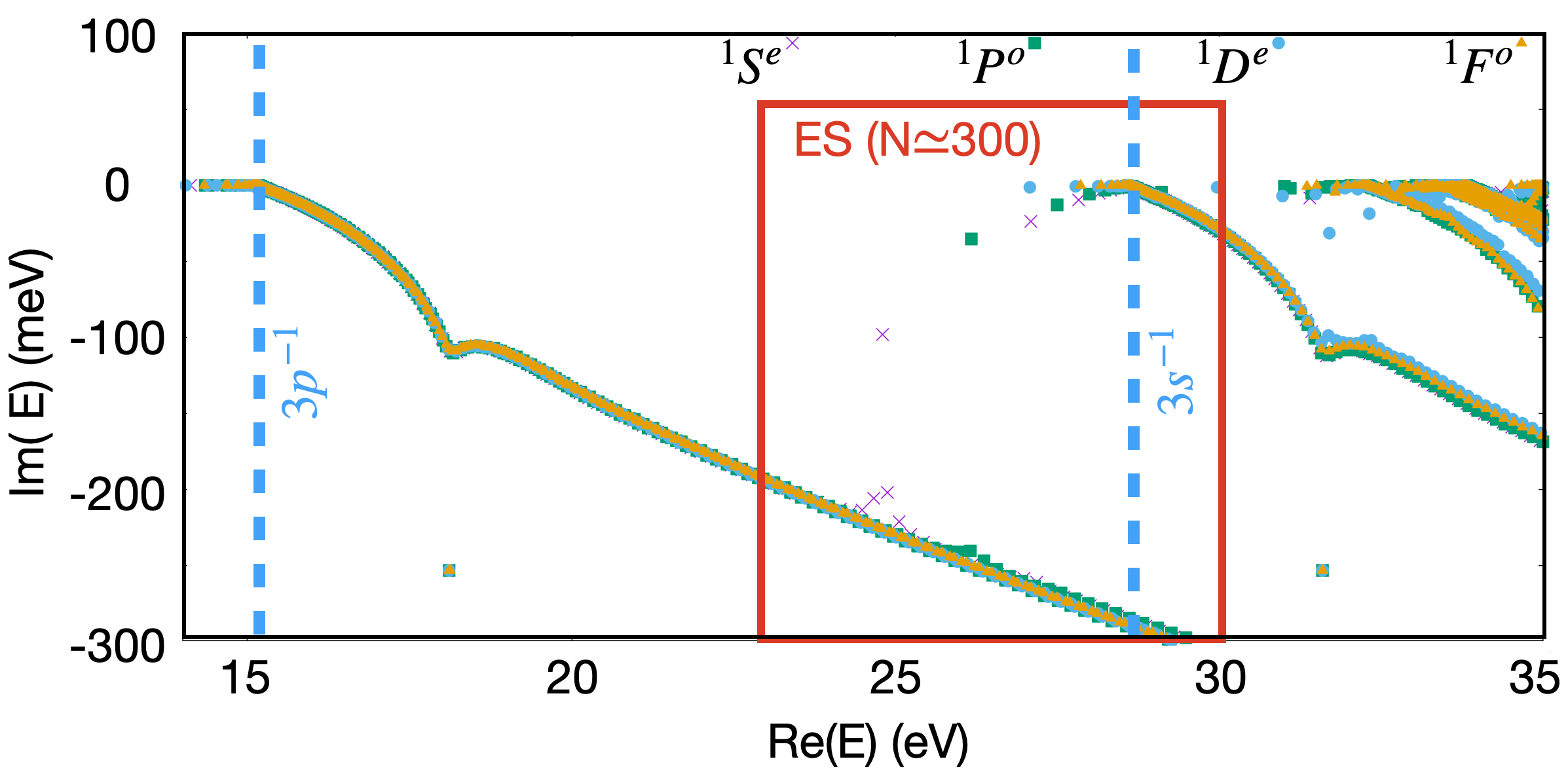
Figure 8: Depiction of states retained from close-coupling calculations for the essential states basis, with symmetry ${}^{1}S^{e}$ (crosses, magenta online), ${}^{1}P^{o}$ (full square, green online), ${}^{1}D^{e}$ (full circles, cyan online), and ${}^{1}F^{o}$ (full triangles, orange online).

Figure 8 shows a section of the complex spectrum of the quenched Hamiltonian in ${}^{1}S^{e}$, ${}^{1}P^{o}$, ${}^{1}D^{e}$, and ${}^{1}F^{o}$ symmetry. In the figure, we can clearly distinguish three main types of eigenvalues: bound states (with zero imaginary part, located below the first ionization threshold), discretized continuum states (branching off from the real axis at each channel’s threshold $E_{\mathrm{th}}$ with increasingly negative imaginary parts), and autoionizing states.

The energies of the autoionizing Feshbach resonances are recognizable as they form Rydberg series converging to the thresholds defined by the excited ionic states. These energies can be expressed as $\bar{E}_{i}=E_{\mathrm{th}}-1/[2(n_{i}-\mu_{i})^{2}]$, where $n_{i}$ is the principal quantum number and $\mu_{i}$ the quantum defect Aymar et al. (1996). The width of these states decreases with the cube of the effective quantum number $n_{i}-\mu_{i}$, as $\lim_{i\to\infty}{(n_{i}-\mu_{i})^{3}}\,\Gamma_{i}=\bar{\Gamma}_{\infty}>0$. Given that the computational cost of a simulation in a spectral basis grows rapidly (at least quadratically) with the basis size, and considering that the XUV transient absorption spectrum primarily probes the inner region of the wave function, we observed that the basis size can be significantly reduced (to less than 1% of the original size) without affecting the quality of the simulated absorption spectrum.

To construct the essential states basis, we eliminate eigenvectors from the close-coupling basis whose energies fall outside a region expected to be accessed by the pump-probe sequence (as illustrated in Figure 8). We retain the eigenvalues and dipole matrix elements obtained from the full structure calculation for the remaining states that compose the essential states basis. We illustrate the robustness of the simulation to this basis reduction by comparing the results of the time-dependent calculations computed in both the full close-coupling basis and in the essential states basis. We employ a split-exponential propagator for this purpose,

$$\begin{split}|\Psi(t+dt)\rangle&=U(t+dt)|\Psi(t)\rangle\\ U(t+dt)&=e^{-i\frac{dt}{2}H_{0}}e^{-i\alpha dt\vec{A}(t+\frac{dt}{2})\cdot\vec{p}}e^{-i\frac{dt}{2}H_{0}}.\end{split}$$ (54)

In the full ab initio calculations, the dipole interaction term is estimated using an iterative Krylov solver, while in the essential states basis, the dipole-interaction Hamiltonian can be diagonalized at the outset. The absorption spectrum, or optical density (OD), is then calculated in the velocity gauge as:

$$\sigma(\omega)=-\frac{4\pi}{\omega}\imaginary\left[\frac{p(\omega)}{A(\omega)}\right],$$ (55)

where $p(\omega)$ and $A(\omega)$ are the Fourier tranform of the expectation value of the electronic momentum $p(t)=\langle\Psi(t)|p_{z}|\Psi(t)\rangle$ and of the vector potential of the external field, respectively. Both sets of calculations yield nearly identical results, as shown in figure 9.

As highlighted earlier, in the essential-state basis, the energies of the autoionizing states are isolated points in the complex plane. This representation enables us to identify these states and, when necessary, alter their parameters (energy and width) to align with experimental values or selectively exclude certain states. This capability is crucial for both identifying the mechanisms underlying specific spectral features and achieving quantitative agreement with experimental data. Indeed, absorption spectra are highly sensitive to the detuning between autoionizing states. If the theory uses the same nominal value for the laser frequency as in the experiment, therefore, it may be necessary to adjust the resonance positions in the calculation to match the experimental values.

This need for adjustment is exemplified by the ab initio calculated energies of the $3s^{-1}3d$, $3s^{-1}5s$, and $3s^{-1}6p$ resonances, which slightly differ from their experimental counterparts in terms of the energy distance from the $3s^{-1}3p$ state, as shown in table 1.

Table 1: Comparison between the theoretical (th) and experimental (exp) energy separation $\Delta E$ of certain relevant resonances from the $3s^{-1}4p$ state.

AIS	$\Delta E_{\mathrm{th}}$ (eV)	$\Delta E_{\mathrm{exp}}$ (eV)
$3s^{-1}3d$	0.91	0.89
$3s^{-1}5s$	0.92	0.93
$3s^{-1}6p$	1.82	1.90

Consequently, in our calculations, we adjust the positions of those resonances so that their detuning from the $3s^{-1}4p$ state matches the experimental conditions Ke-Zun et al. (2003); Carette et al. (2013). Ideally, we would also adjust the position of the $3s^{-1}4f$, but, to the best of our knowledge, there is no reported experimental value for this resonance in the literature.

Figure 9 presents a comparative analysis of the theoretical transient absorption spectrum of argon in the vicinity of the $3s^{-1}4p$ resonance, as a function of the pump-probe delay, for several values of the IR frequency. These simulations were conducted using a 4 fs XUV pulse centered on the $3s^{-1}4p$ and a 50 fs IR pulse with a peak intensity of 40 GW/cm².

Three different bases were employed for these simulations. The first, an (ab initio) basis, includes all close-coupling states, amounting to an order of $10^{4}$ states. The second basis, labelled ES (Essential States), encompasses a selective set of about $10^{2}$ essential states. The third basis, ES-shifted, maintains the same states as the ES basis but adjusts the energy of the resonances listed in table 1. This adjustment aligns their separation from the $3s^{-1}4p$ state with experimental values, and simultaneously modifies the IR energy to ensure that the detuning $\delta=E_{3s^{-1}3d}-E_{3s^{-1}4p}-\omega_{\textsc{IR}}$ remains consistent across all calculations.

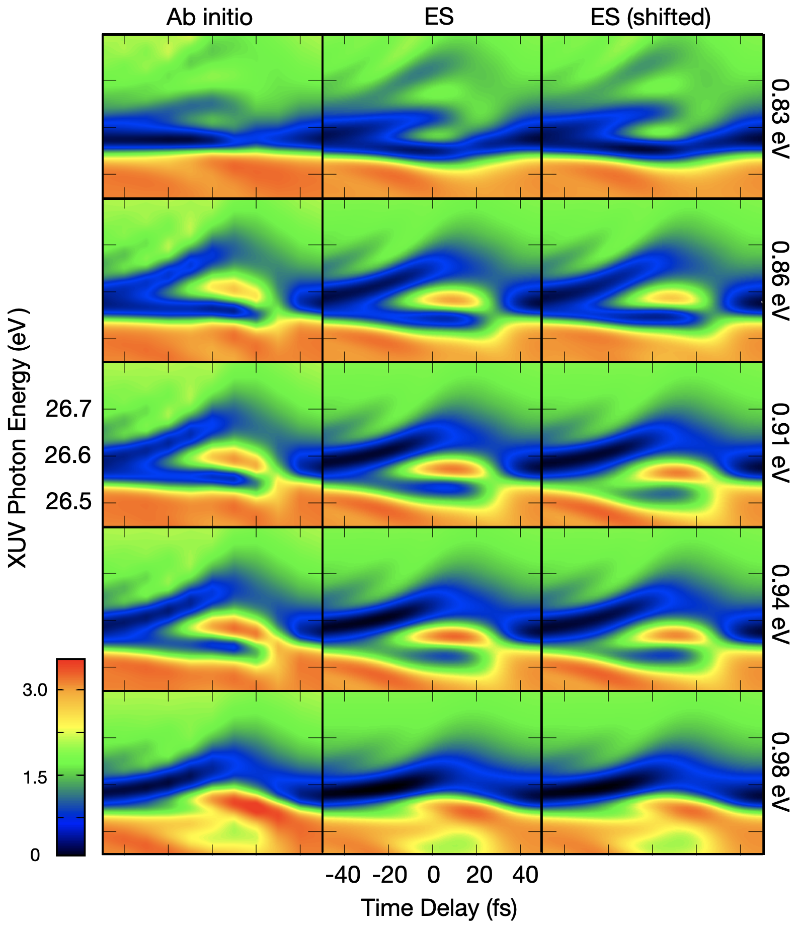
Figure 9: Comparison of ab initio calculation of the absorption spectrum as a function of time delay (left) at various IR energies with results from the essential states model. In the middle, resonance positions are kept as computed; on the right, they are shifted to match experimentally measured energies, with the IR energy adjusted to maintain constant $3s^{-1}4p-3s^{-1}3d$ detuning. Listed IR energies correspond to the unshifted calculations. In the top (bottom) row, the IR is tuned below (above) the resonant transition, positioning the light-induced states above (below) the $3s^{-1}4p$ resonance.

In all the cases shown in Fig. 9, a global shift of 0.405 eV is applied to the XUV photon energy to align the position of the $3s^{-1}4p$ with its experimentally observed value Harkema et al. (2021). To account for the finite spectrometer resolution in experiments, the simulation results are convoluted with a Gaussian function having a full width at half maximum (FWHM) of 25 meV.

As the IR is tuned to the $4p-3d$ transition (middle row), the $4p$ state splits into a pair of autoionizing polaritons due to the IR intensity and the strong coupling between the resonances. The polaritonic branches significantly differ in their widths, which are modulated by the time delay of the IR.

The comparison between the ab initio (left column) and the Essential States (ES, middle column) calculations in Figure 9 shows how excluding up to 99% of the basis states does not significantly alter the simulation results. This demonstrates the robustness and efficiency of the ES approach in capturing the essential dynamics of the system.

Furthermore, the comparison between the ES (middle column) and the shifted ES (right column) calculations highlights the paramount importance of the detuning between the IR dressing field and the energy separation of different resonances. As observed, when the detuning is consistent across calculations, the spectral shapes in the central and right columns are remarkably similar. This result shows that with the ES approach it is possible to match the frequency of the IR to its nominal experimental value while also preserving the same detuning as in the experiment.

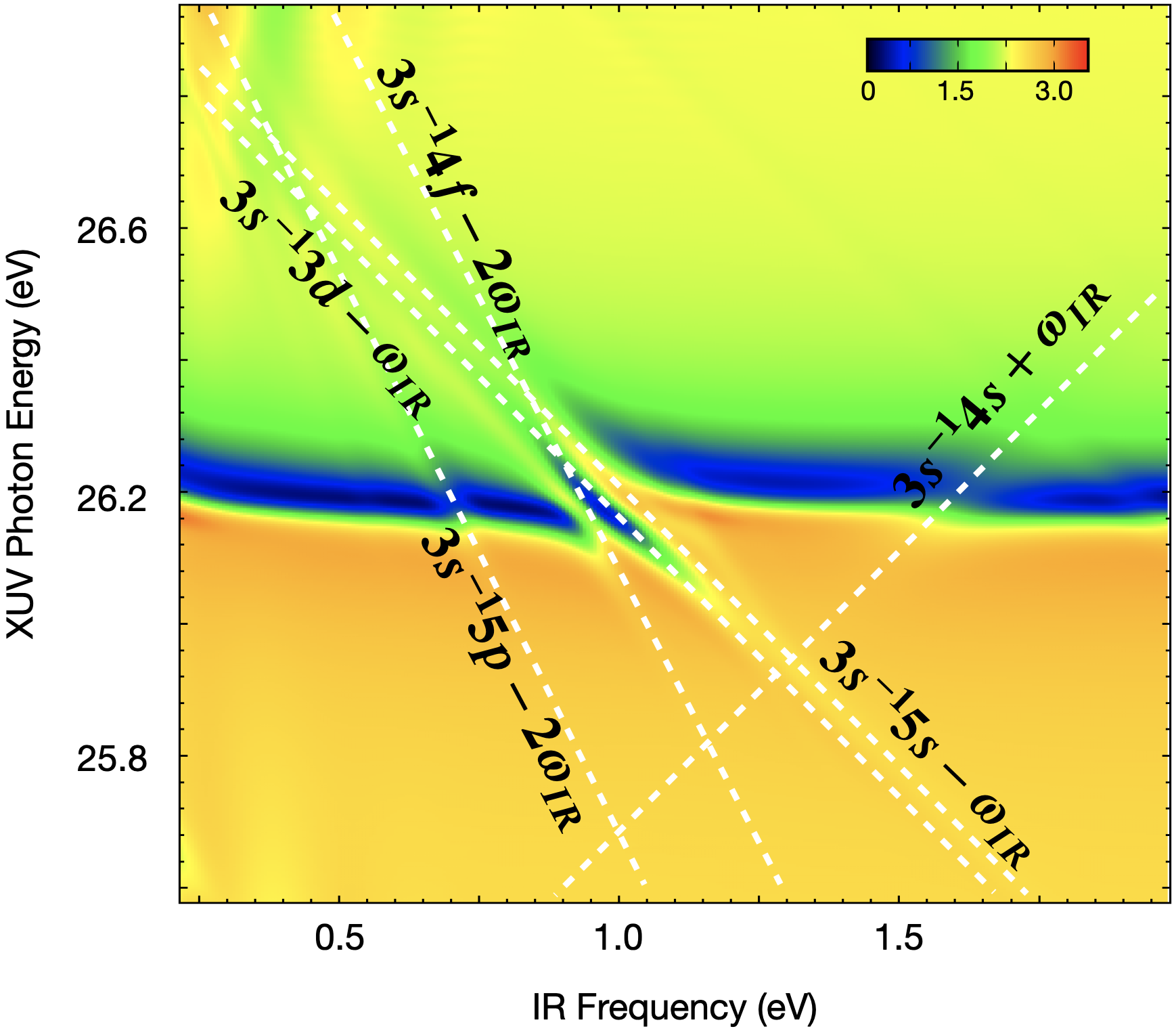
Figure 10: Ab initio calculation of the absorption spectrum $\sigma(\omega_{\textsc{xuv}};\omega_{\textsc{ir}},I_{\textsc{ir}},\tau)$ at time delay $\tau=0$, as a function of the dressing laser frequency $\omega_{\textsc{IR}}$. The nominal position of the various LIS as a function of $\omega_{\textsc{IR}}$, $E_{3s^{-1}n\ell+n\gamma_{\textsc{IR}}}(\omega_{\textsc{IR}})=E_{3s^{-1}n\ell}+n\hbar\omega_{\textsc{IR}}$, are marked with white dashed lines and labelled according to their corresponding resonances. The figure clearly shows the avoided crossing between these LIS states and the bright $3s^{-1}4p$ window resonance.

Figure 10 shows the absorption spectrum $\sigma(\omega_{\textsc{xuv}};\omega_{\textsc{ir}},I_{\textsc{ir}},\tau)$ as a function of the dressing-laser frequency. In this range of IR energies we can observe the effect of several one and two-photon couplings between the $3s^{-1}4p$ and other resonances in the continuum, which manifest themselves as avoided crossings. The nominal energies $E_{a}\pm n\omega_{\textsc{IR}}$ of the LIS corresponding to each dark state $a$ coupled to the ${}^{1}P^{o}$ symmetry by an $n$-photon transition, is indicated on the frequency map with a white dashed line. As the figure shows, these lines intersect the main $3s^{-1}4p$ signal right where the avoided crossings appear. In particular, in the frequency interval around $\omega_{\textsc{IR}}\simeq$1 eV, as many as three LIS overlap with the bright state, giving rise to a complex polaritonic multiplet.

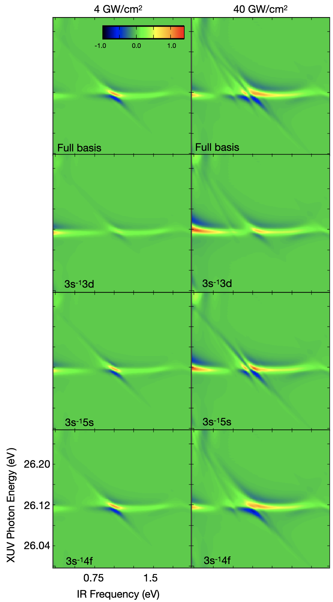
Figure 11: Normalized transient absorption signal, represented as $\Delta\sigma\,I_{0}/I_{\textsc{IR}}$ with $I_{0}=$40 GW/cm², as a function of the dressing laser frequency at a fixed zero time delay. The signal is computed ab initio for two different peak intensities of the dressing laser field: 4 GW/cm², 40 GW/cm². The figure is organized to demonstrate the impact of different basis configurations on the absorption signal. The top row presents results computed using the full basis. Subsequent rows illustrate the effect of selectively omitting certain autoionizing states from the basis- specifically, the $3s^{-1}3d$, $3s^{-1}5s$, and $3s^{-1}4f$ states.

To determine which transitions contribute to the observed spectral features, we selectively exclude specific autoionizing states in our simulations with the essential-states basis. Figure 11 demonstrates this method by presenting a normalized transient absorption signal, $\Delta\sigma$, defined as $\Delta\sigma=\Delta\sigma(\omega_{\textsc{xuv}};\omega_{\textsc{ir}},I_{\textsc{ir}},\tau)\equiv\sigma(\omega_{\textsc{xuv}};\omega_{\textsc{ir}},I_{\textsc{ir}},\tau)-\sigma(\omega_{\textsc{xuv}};\omega_{\textsc{ir}},I_{\textsc{ir}},-\infty)$. This signal is obtained using either the full basis or by omitting one of the AIS that lead to a relevant LIS, at two different intensities of the dressing laser, $I_{\textsc{IR}}=4$ GW/cm² and $I_{\textsc{IR}}=40$ GW/cm².

Since $\Delta\sigma$ scales linearly with the laser intensity to lowest order, the $\Delta\sigma$ for $I_{\textsc{IR}}=4$ GW/cm² has been scaled by a factor of 10 for easier comparison with the spectrum computed at the higher intensity. At the lowest intensity, LIS associated with two-photon transitions are barely discernible. Indeed, removing the $3s^{-1}4f$ state from the simulation at $I_{\textsc{IR}}=4$ GW/cm² has a negligible effect on the spectrum. We also notice that the stronger change in the spectrum is due to the $3s^{-1}3d$ state.

At higher intensities, the spectrum develops features associated to two new LIS. As suggested by Fig. 10, the feature intersecting the avoided crossing between the $3s^{-1}4p$, $3s^{-1}5s$, and $3s^{-1}3d$ states is likely due to the $3s^{-1}4f$ LIS. Indeed, by eliminating this AIS from the basis, that feature disappears. A similar calculation enables us to attribute the second new feature, intersecting the $3s^{-1}4p$ line at approximately $\omega_{\textsc{IR}}\simeq 0.75$ eV, to the $3s^{-1}5p$ AIS.

V Conclusions

In this work, we have successfully developed an analytical model that integrates the Jaynes-Cummings formalism with Fano’s formalism to describe the optical response of laser-dressed autoionizing states. We use the JC model to quantify the splitting of strongly coupled autoionizing resonances as a function of the driving laser parameters, and explain how competing radiative and Auger ionization pathways can result in the stabilization of an autoionizing polariton. The predictions of the JC model regarding polaritonic formation and of resonance stabilization have been corroborated by ab initio simulations conducted in an essential-states basis. This methodological approach has proven to be highly efficient, accelerating calculations by three or more orders of magnitude compared to those carried out in a full close-coupling basis, without compromising the accuracy of the results. The essential-state approach also facilitates the identification of the crucial states that should be included in a realistic modeling of the system. Finally, the JC model provides analytical expressions for the line shapes of overlapping laser-dressed autoionizing states in transient absorption spectra. These expressions are useful tools for extracting key system parameters, such as resonance widths, from experimental data.

VI Acknowledgements

We gratefully acknowledge the support received for this work. LA and SM thank the National Science Foundation’s Theoretical AMO Physics program for their support through grants No. 1607588 and No. 1912507. EL acknowledges support from the Swedish Research Council under Grant No. 2020-03315. The authors are grateful for the computational resources provided by the UCF ARCC. Additionally, AS, NH, and SP acknowledge the support from the U.S. Department of Energy, Office of Science, Basic Energy Sciences, under Award No. DE-SC0018251.

References

- Berrah et al. (1996) N Berrah, B Langer, J Bozek, T W Gorczyca, O Hemmers, D W Lindle, and O Toader, “Angular-distribution parameters and R -matrix calculations of Ar resonances,” J. Phys. B At. Mol. Opt. Phys. 29, 5351–5365 (1996).
- Lukin and Imamoğlu (2001) M. D. Lukin and A. Imamoğlu, “Controlling photons using electromagnetically induced transparency,” Nature 413, 273–276 (2001).
- Fleischhauer et al. (2005) Michael Fleischhauer, Atac Imamoglu, and P. Jonathan Marangos, “Electromagnetically induced transparency,” Rev. Mod. Phys. 77, 633–673 (2005).
- Pazourek et al. (2015) Renate Pazourek, Stefan Nagele, and Joachim Burgd?rfer, “Probing time-ordering in two-photon double ionization of helium on the attosecond time scale,” J. Phys. B: At. Mol. Opt. Phys. 48, 061002 (2015).
- Goulielmakis et al. (2010) Eleftherios Goulielmakis, Zhi-Heng Loh, Adrian Wirth, Robin Santra, Nina Rohringer, Vladislav S. Yakovlev, Sergey Zherebtsov, Thomas Pfeifer, Abdallah M. Azzeer, Matthias F. Kling, Stephen R. Leone, and Ferenc Krausz, “Real-time observation of valence electron motion,” Nature 466, 739–743 (2010).
- Månsson et al. (2014) Erik P. Månsson, Diego Guénot, Cord L. Arnold, David Kroon, Susan Kasper, J. Marcus Dahlström, Eva Lindroth, Anatoli S. Kheifets, Anne L’Huillier, Stacey L. Sorensen, and Mathieu Gisselbrecht, “Double ionization probed on the attosecond timescale,” Nature Physics 10, 207–211 (2014).
- Jiménez-Galán et al. (2014) Álvaro Jiménez-Galán, Luca Argenti, and Fernando Martín, “Modulation of Attosecond Beating in Resonant Two-Photon Ionization,” Phys. Rev. Lett. 113, 263001 (2014).
- Argenti et al. (2015) L. Argenti, Á. Jiménez-Galán, C. Marante, C. Ott, T. Pfeifer, and F. Martín, “Dressing effects in the attosecond transient absorption spectra of doubly excited states in helium,” Phys. Rev. A 91, 061403 (2015).
- Kotur et al. (2016) Marija Kotur, D. Guénot, Álvaro Jiménez-Galán, David Kroon, E W Larsen, M Louisy, S. Bengtsson, M Miranda, J Mauritsson, C L Arnold, S E Canton, M Gisselbrecht, T Carette, J. M. Dahlström, Eva Lindroth, Alfred Maquet, Luca Argenti, Fernando Martín, and A. L’Huillier, “Spectral phase measurement of a Fano resonance using tunable attosecond pulses,” Nature Commun. 7, 10566 (2016), 1505.02024 .
- Lin and Chu (2013) C D Lin and Wei-Chun Chu, “Controlling Atomic Line Shapes,” Science 340, 694–695 (2013).
- Ossiander et al. (2016) M. Ossiander, F. Siegrist, V. Shirvanyan, R. Pazourek, A. Sommer, T. Latka, A. Guggenmos, S. Nagele, J. Feist, J. Burgdörfer, R. Kienberger, and M. Schultze, “Attosecond Correlation Dynamics,” Nature Physics 13, 280 (2016).
- Chu and Lin (2010) W.-C. Chu and C. D. Lin, “Theory of ultrafast autoionization dynamics of Fano resonances,” Phys. Rev. A 82, 053415 (2010).
- Douguet et al. (2016) Nicolas Douguet, Alexei N. Grum-Grzhimailo, Elena V. Gryzlova, Ekaterina I. Staroselskaya, Joel Venzke, and Klaus Bartschat, “Photoelectron angular distributions in bichromatic atomic ionization induced by circularly polarized VUV femtosecond pulses,” Phys. Rev. A 93, 033402 (2016).
- Barreau et al. (2016) L Barreau, F Risoud, J Caillat, A Maquet, F Lepetit, T Ruchon, L Argenti, and Laboratoire De Chimie Physique, “Attosecond dynamics through a Fano resonance: Monitoring the birth of a photoelectron,” Science 354, 734–738 (2016).
- Xie et al. (2012) Xinhua Xie, Katharina Doblhoff-Dier, Stefan Roither, Markus S. Schöffler, Daniil Kartashov, Huailiang Xu, Tim Rathje, Gerhard G. Paulus, Andrius Baltuska, Stefanie Gräfe, and Markus Kitzler, “Attosecond-recollision-controlled selective fragmentation of polyatomic molecules,” Phys. Rev. Lett. 109, 243001 (2012).
- Joffre (2007) Manuel Joffre, “Comment on ”Coherent Control of Retinal Isomerization in Bacteriorhodopsin”,” Science 317, 453 (2007).
- Peng et al. (2015) Liang You Peng, Wei Chao Jiang, Ji Wei Geng, Wei Hao Xiong, and Qihuang Gong, “Tracing and controlling electronic dynamics in atoms and molecules by attosecond pulses,” Phys. Rep. 575, 1–71 (2015).
- Wang et al. (2021) Xuanhua Wang, Zhedong Zhang, and Jin Wang, “Excitation-energy transfer under strong laser drive,” Phys. Rev. A 103, 013516 (2021).
- Asenjo-Garcia et al. (2017) A. Asenjo-Garcia, M. Moreno-Cardoner, A. Albrecht, H. J. Kimble, and D. E. Chang, “Exponential improvement in photon storage fidelities using subradiance & ”selective radiance” in atomic arrays,” Phys. Rev. X 7, 031024 (2017).
- Haessler et al. (2010) S. Haessler, J. Caillat, W. Boutu, C. Giovanetti-Teixeira, T. Ruchon, T. Auguste, Z. Diveki, P. Breger, a. Maquet, B. Carré, R. Taïeb, and P. Salières, “Attosecond imaging of molecular electronic wavepackets,” Nature Physics 6, 200–206 (2010).
- Lépine et al. (2014) Franck Lépine, Misha Y. Ivanov, and Marc J. J. Vrakking, “Attosecond molecular dynamics: fact or fiction?” Nature Photonics 8, 195–204 (2014).
- Huppert et al. (2016) Martin Huppert, Inga Jordan, Denitsa Baykusheva, Aaron Von Conta, and Hans Jakob Wörner, “Attosecond Delays in Molecular Photoionization,” Phys. Rev. Lett. 117, 093001 (2016).
- Sidiropoulos et al. (2022) T.P.H. Sidiropoulos, N. Di Palo, D.E. Rivas, S. Severino, M. Reduzzi, B. Nandy, B. Bauerhenne, S. Krylow, T. Vasileiadis, T. Danz, P. Elliott, S. Sharma, K. Dewhurst, C. Ropers, Y. Joly, K. M. E. Garcia, M. Wolf, R. Ernstorfer, and J. Biegert, “Real-time flow of excitation inside a material with attosecond core-level soft x-ray spectroscopy,” in Optica High-brightness Sources and Light-driven Interactions Congress 2022 (Optica Publishing Group, 2022) p. HF5B.1.
- Krüger et al. (2011) Michael Krüger, Markus Schenk, and Peter Hommelhoff, “Attosecond control of electrons emitted from a nanoscale metal tip,” Nature 475, 78–81 (2011).
- Fan et al. (2022) G. Fan, K. Légaré, V. Cardin, X. Xie, R. Safaei, E. Kaksis, G. Andriukaitis, A. Pugžlys, B. E. Schmidt, J. P. Wolf, M. Hehn, G. Malinowski, B. Vodungbo, E. Jal, J. Lüning, N. Jaouen, G. Giovannetti, F. Calegari, Z. Tao, A. Baltuška, F. Légaré, and T. Balčiūnas, “Ultrafast magnetic scattering on ferrimagnets enabled by a bright yb-based soft x-ray source,” Optica 9, 399–407 (2022).
- Lindroth and Argenti (2012) E. Lindroth and L. Argenti, “Atomic resonance states and their role in charge-changing processes,” Adv. Quant. Chem. 63, 247 (2012).
- Fano and Cooper (1965) U. Fano and J. W. Cooper, “Line profiles in the far-uv absorption spectra of the rare gases,” Phys. Rev. 137, A1364–A1379 (1965).
- Gruson et al. (2016) V. Gruson, L. Barreau, Á. Jiménez-Galan, F. Risoud, J. Caillat, A. Maquet, B. Carré, F. Lepetit, J.-F. Hergott, T. Ruchon, L. Argenti, R. Taïeb, F. Martín, and P. Salières, “Attosecond dynamics through a fano resonance: Monitoring the birth of a photoelectron,” Science 354, 734–738 (2016).
- Ott et al. (2013) Christian Ott, Andreas Kaldun, Philipp Raith, Kristina Meyer, Martin Laux, Jörg Evers, Christoph H. Keitel, Chris H. Greene, and Thomas Pfeifer, “Lorentz meets fano in spectral line shapes: A universal phase and its laser control,” Science 340, 716–720 (2013).
- Chini et al. (2012) Michael Chini, Baozhen Zhao, He Wang, Yan Cheng, S. X. Hu, and Zenghu Chang, “Subcycle ac stark shift of helium excited states probed with isolated attosecond pulses,” Phys. Rev. Lett. 109, 073601 (2012).
- Chini et al. (2013) Michael Chini, Xiaowei Wang, Yan Cheng, Yi Wu, Di Zhao, Dmitry a Telnov, Shih-I Chu, and Zenghu Chang, “Sub-cycle Oscillations in Virtual States Brought to Light,” Sci. Rep. 3, 1105 (2013).
- Yang et al. (2015) Z. Q. Yang, D. F. Ye, Thomas Ding, Thomas Pfeifer, and L. B. Fu, “Attosecond XUV absorption spectroscopy of doubly excited states in helium atoms dressed by a time-delayed femtosecond infrared laser,” Phys. Rev. A 91, 013414 (2015).
- Ott et al. (2014) Christian Ott, Andreas Kaldun, Luca Argenti, Philipp Raith, Kristina Meyer, Martin Laux, Yizhu Zhang, Alexander Blättermann, Steffen Hagstotz, Thomas Ding, Robert Heck, Javier Madroñero, Fernando Martín, and Thomas Pfeifer, “Reconstruction and control of a time-dependent two-electron wave packet,” Nature 516, 374 (2014).
- Zhao et al. (2017) Haiwen Zhao, Candong Liu, Yinghui Zheng, Zhinan Zeng, and Ruxin Li, “Attosecond chirp effect on the transient absorption spectrum of laser-dressed helium atom,” Opt. Exp. 25, 7707 (2017).
- Wang et al. (2010) He Wang, Michael Chini, Shouyuan Chen, Chang Hua Zhang, Feng He, Yan Cheng, Yi Wu, Uwe Thumm, and Zenghu Chang, “Attosecond time-resolved autoionization of argon,” Phys. Rev. Lett. 105, 143002 (2010).
- Pfeiffer and Leone (2012) Adrian N. Pfeiffer and Stephen R. Leone, “Transmission of an isolated attosecond pulse in a strong-field dressed atom,” Phys. Rev. A 85, 053422 (2012).
- Kobayashi et al. (2017) Yuki Kobayashi, Henry Timmers, Mazyar Sabbar, Stephen R Leone, and Daniel M Neumark, “Attosecond transient-absorption dynamics of xenon core-excited states in a strong driving field,” Phys. Rev. A 95, 031401 (2017).
- Mihelič et al. (2017) Andrej Mihelič, Matjaž Žitnik, and Mateja Hrast, “Doubly resonant photoionization of he below the n= 2 ionization threshold,” J. Phys. B: At. Mol. Opt. Phys. 50, 245602 (2017).
- Gaarde et al. (2011) Mette B. Gaarde, Christian Buth, Jennifer L. Tate, and Kenneth J. Schafer, “Transient absorption and reshaping of ultrafast XUV light by laser-dressed helium,” Phys. Rev. A 83, 013419 (2011).
- Wu et al. (2013) Mengxi Wu, Shaohao Chen, Mette B. Gaarde, and Kenneth J. Schafer, “Time-domain perspective on Autler-Townes splitting in attosecond transient absorption of laser-dressed helium atoms,” Phys. Rev. A 88, 043416 (2013).
- Jaynes and Cummings (1963) E. T. Jaynes and F. W. Cummings, “Comparison of quantum and semiclassical radiation theories with application to the beam maser,” Proc. IEEE 51, 89–109 (1963).
- Galego et al. (2015) Javier Galego, Francisco J. Garcia-Vidal, and Johannes Feist, “Cavity-induced modifications of molecular structure in the strong-coupling regime,” Phys. Rev. X 5, 041022 (2015).
- Zhang et al. (2019) Zhedong Zhang, Kai Wang, Zhenhuan Yi, M. Suhail Zubairy, Marlan O. Scully, and Shaul Mukamel, “Polariton-assisted cooperativity of molecules in microcavities monitored by two-dimensional infrared spectroscopy,” The Journal of Physical Chemistry Letters 10, 4448–4454 (2019).
- Herrera and Owrutsky (2020) Felipe Herrera and Jeffrey Owrutsky, “Molecular polaritons for controlling chemistry with quantum optics,” The Journal of Chemical Physics 152, 100902 (2020).
- Harkema et al. (2021) N. Harkema, C. Cariker, E. Lindroth, L. Argenti, and A. Sandhu, “Autoionizing polaritons in attosecond atomic ionization,” Phys. Rev. Lett. 127, 023202 (2021).
- Kim and Lambropoulos (1982) Young Soon Kim and P. Lambropoulos, “Laser-intensity effect on the configuration interaction in multiphoton ionization and autoionization,” Phys. Rev. Lett. 49, 1698–1701 (1982).
- Peng et al. (2020) Yun Peng, Yong Zhao, Xu guang Hu, and Yang Yang, “Optical fiber quantum biosensor based on surface plasmon polaritons for the label-free measurement of protein,” Sensors and Actuators, B: Chemical 316, 128097 (2020).
- Song et al. (2016) Xue Ke Song, Qing Ai, Jing Qiu, and Fu Guo Deng, “Physically feasible three-level transitionless quantum driving with multiple Schrödinger dynamics,” Phys. Rev. A 93, 052324 (2016).
- Carette et al. (2013) T. Carette, J. M. Dahlström, L. Argenti, and E. Lindroth, “Multiconfigurational Hartree-Fock close-coupling ansatz: Application to the argon photoionization cross section and delays,” Phys. Rev. A 87, 023420 (2013).
- Yanez-Pagans et al. (2022) S. Yanez-Pagans, C. Cariker, M. Shaikh, L. Argenti, and A. Sandhu, “Multipolariton control in attosecond transient absorption of autoionizing states,” Phys. Rev. A 105, 063107 (2022).
- Sakurai (1994) Jun John Sakurai, Modern quantum mechanics; rev. ed. (Addison-Wesley, Reading, MA, 1994).
- Cohen-Tannoudji (1996) Claude N. Cohen-Tannoudji, “The Autler-Townes effect revisited,” in Amazing Light: A Volume Dedicated To Charles Hard Townes On His 80th Birthday, edited by Raymond Y. Chiao (Springer New York, New York, NY, 1996) pp. 109–123.
- Cohen-Tannoudji et al. (1989) Claude Cohen-Tannoudji, Jacques Dupont-Roc, and Gilbert Grynberg, Photons and Atoms: Introduction to Quantum Electrodynamics (Wiley, New York, 1989).
- Jackson (1975) John David Jackson, Classical electrodynamics; 2nd ed. (Wiley, New York, NY, 1975).
- Fox (2001) A. M. Fox, Optical Properties of Solids (Oxford University Press, Oxford, UK, 2001).
- Rabi (1937) I. I. Rabi, “Space quantization in a gyrating magnetic field,” Phys. Rev. 51, 652–654 (1937).
- Fano (1961) U. Fano, “Effects of Configuration Interaction on Intensities and Phase Shifts,” Physical Review 124, 1866–1878 (1961).
- Newton (1966) Roger G. Newton, Scattering theory of waves and particles [by] Roger G. Newton., International series in pure and applied physics (McGraw-Hill, New York, 1966).
- Taylor (1972) J. R. Taylor, Scattering Theory: The quantum Theory on Nonrelativistic Collisions (Wiley, New York, 1972).
- Argenti et al. (2013) Luca Argenti, Renate Pazourek, Johannes Feist, Stefan Nagele, Matthias Liertzer, Emil Persson, Joachim Burgd??rfer, and Eva Lindroth, “Photoionization of helium by attosecond pulses: Extraction of spectra from correlated wave functions,” Phys. Rev. A 87, 053405 (2013), arXiv:1210.2187 .
- C Froese-Fischer (1997) T. Jonsson C Froese-Fischer, C. Brage, Computational Atomic Structure (IOP Publishing, Philadelphia, 1997).
- Argenti and Moccia (2006) Luca Argenti and Roberto Moccia, “K -matrix method with B-splines: , and resonances in He photoionization below N = 4 threshold,” J. Phys. B: At. Mol. Opt. Phys. 39, 2773–2790 (2006).
- Aymar et al. (1996) Mireille Aymar, Chris H. Greene, and Eliane Luc-Koenig, “Multichannel rydberg spectroscopy of complex atoms,” Rev. Mod. Phys. 68, 1015–1123 (1996).
- Ke-Zun et al. (2003) Zhu Lin-Fan Ke-Zun, Cheng Hua-Dong, Liu Xiao-Jing, Tian Peng, Yuan Zhen-Sheng, Li Wen-Bin, and Xu, “Optically Forbidden Excitations of 3 s Electron of Argon by Fast Electron Impact,” Chin. Phys. Lett. 20, 1718 (2003).