Conquering the Communication Constraints to Enable Large Pre-Trained Models in Federated Learning

Abstract

Federated learning (FL) has emerged as a promising paradigm for enabling the collaborative training of models without centralized access to the raw data on local devices. In the typical FL paradigm (e.g., FedAvg), model weights are sent to and from the server each round to participating clients. Recently, the use of small pre-trained models has been shown effective in federated learning optimization and improving convergence. However, recent state-of-the-art pre-trained models are getting more capable but also have more parameters. In conventional FL, sharing the enormous model weights can quickly put a massive communication burden on the system, especially if more capable models are employed. Can we find a solution to enable those strong and readily-available pre-trained models in FL to achieve excellent performance while simultaneously reducing the communication burden? To this end, we investigate the use of parameter-efficient fine-tuning in federated learning and thus introduce a new framework: FedPEFT. Specifically, we systemically evaluate the performance of FedPEFT across a variety of client stability, data distribution, and differential privacy settings. By only locally tuning and globally sharing a small portion of the model weights, significant reductions in the total communication overhead can be achieved while maintaining competitive or even better performance in a wide range of federated learning scenarios, providing insight into a new paradigm for practical and effective federated systems.

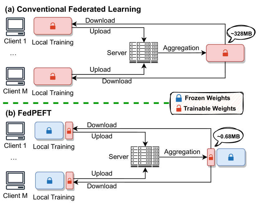
Figure 1: Process in a federated learning communication round with $M$ participating clients. We use ViT-Base as an instance to analyze the communication costs. (a) Conventional federated learning framework, where the entire model will be sent during the communication. (b) FedPEFT, which is our proposed parameter-efficient framework for federated learning. Instead of uploading and downloading the entire model during the communication, only a small subset of the model will be updated and communicated, leading to a huge relief in communication, specifically from about 328MB per round to about 0.68MB per round.

1 Introduction

Federated learning (FL) [29] has become increasingly prevalent in the research community, having the goal of enabling collaborative training with a network of clients without needing to share any private data. One key challenge for this training paradigm is overcoming data heterogeneity. The participating devices in a federated system are often deployed across a variety of users and environments, resulting in a non-IID data distribution. As the level of heterogeneity intensifies, optimization becomes increasingly difficult. Various techniques have been proposed for alleviating this issue. These primarily consist of modifications to the local or global objectives through proximal terms, regularization, and improved aggregation operations [26, 21, 30, 1, 42]. More recently, some works have investigated the role of model initialization in mitigating such effects [31, 7]. Inspired by the common usage of pre-trained models for facilitating strong transfer learning in centralized training, researchers employed widely-available pre-trained weights for initialization in FL and were able to close much of the gap between federated and centralized performance.

Still, while pre-trained initializations are effective for alleviating heterogeneity effects in FL, another key challenge is left unaddressed; that is, communication constraints. This is often the primary bottleneck for real-world federated systems [20]. In the standard FL framework [29], updates for all model parameters are sent back and forth between the server and participating clients each round. This can quickly put a massive communication burden on the system, especially if more capable models beyond very small MLPs are used.

When employing strong pre-trained models, the number of parameters can be large, such as for current state-of-the-art transformers. For example, ViT-Base (ViT-B) [11] has 84 million parameters, which would simply exacerbate the communication overhead to insurmountable levels. As a compromise, most existing FL work focuses on the performance of smaller Convolutional Neural Networks (e.g., ResNet [17]) on smaller datasets (e.g., CIFAR-10 [23], EMINIST [9]). Considering the thriving progress in large pre-trained Foundation Models [2], an efficient framework enabling these large pre-trained models will be significant for the FL community.

Based on the previous study on centralized training [3, 19, 33, 6], we note that pre-trained models have strong representations, and updating all the weights during fine-tuning is often not necessary. Various parameter-efficient fine-tuning methods (e.g., fine-tuning only a subset of the parameters or the bias terms) for centralized training have been proposed in the literature and show that successful and efficient adaptation is possible, even under domain shift [19, 3, 33]. We reason that such insight is applicable to FL, where each client can be thought of as a shifted domain on which we are fine-tuning. By leveraging pre-trained weights, it may be possible to simply update a small portion of the weights for each client. This will significantly reduce the communication burden on the system, as the updates communicated with the server will consist of just a fraction of the total model parameters.

Can we reap these potential communication benefits while still achieving strong performance in FL? Unfortunately, operating conditions in FL are difficult, requiring successful convergence under varying data heterogeneity levels, random client availability, and differential privacy procedures. Therefore, we are unable to properly assess this possibility of benefit based on existing literature, as the effectiveness of parameter-efficient fine-tuning methods has not been explored in such situations in FL. To fill this gap, we explore the viability of a Federated Parameter-Efficient Fine-Tuning (FedPEFT) framework with a systemic empirical study on a comprehensive set of FL scenarios. The framework is illustrated in Figure 1. We deploy parameter-efficient fine-tuning methods to adapt pre-trained models and enable massive reductions in communication overheads. The contribution of this paper can be summarized as follows.

• We introduce FedPEFT, a new federated learning framework that simultaneously addresses data heterogeneity and communication challenges. FedPEFT is the first federated learning framework that enables the leveraging of strong pre-trained models in FL while maintaining an extremely low communication cost.

• We present a systematic study of the FedPEFT framework with various fine-tuning methods under heterogeneous data distributions, client availability ratios, and increasing degrees of domain gap relative to the pre-trained representations on various datasets, showing the capability of FedPEFT. (Sections 5 and 6)

• To ensure FedPEFT is practical for the complex environments of FL, we further analyze the robustness of FedPEFT among low-data regimes, differential privacy operations, and an ablation study with different pre-trained backbones. (Sections 7 and 8)

2 Related Work

Federated Learning. Federated learning is a decentralized training paradigm composed of two procedures: local training and global aggregation. Therefore, most existing work focuses on either local training [30, 25, 26] or global aggregation [43, 46] to learn a better global model. Another line of work cuts into this problem by applying different initialization to help both procedures. [7] show that initializing the model with pre-trained weights can make the global aggregation of FedAvg more stable, even when pre-trained with synthetic data. Furthermore, [31] present the effectiveness of pre-training with different local and global operations. However, these works focus purely on the effect of initialization in a standard FedAvg framework and do not consider the communication constraints of the system. Our work pushes the envelope further by leveraging strong pre-trained models (even large, capable transformers) in federated learning while effectively handling the communication issue via parameter-efficient fine-tuning.

Communication in Federated Learning. Communication constraints are a primary bottleneck in federated learning. To reduce the communication cost, several previous work leverage model compression techniques [22, 38]. Such works do not change the training paradigm but rather post-processes the local model to reduce communication costs. For instance, [22] propose approaches that parameterize the model with fewer variables and compress the model in an encoding-decoding fashion. However, the minimal requirement to maintain all the information is still high when facing today’s large models. Meanwhile, another line of work changes the training paradigm by learning federated ensembles based on several pre-trained base models [15]. In this way, only the mixing weights of the base models will be communicated in each round. This approach aims to reduce the burden of downloading and uploading the entire model in each round. However, the base models are not directly trained, and the final performance is highly related to the base models. Meanwhile, model ensembles will take more time and space, which is often limited on the client side. Our framework follows the strategy of this line of work that does not transmit the entire model, but we use only one pre-trained model instead of several base models and only transmit a subset of the parameters instead of the model ensembles. Therefore, no additional time or space is required.

Parameter-Efficient Fine-tuning. Fine-tuning is a prevalent topic in centralized transfer learning, especially in this era of the “Foundation Model” [2]. A significant line of work is to reduce the trainable parameter number, i.e., parameter-efficient fine-tuning (PEFT) [6, 32, 27]. This enables easier access and usage of pre-trained models by reducing the memory cost needed to conduct fine-tuning due to fewer computed gradients. In federated learning, PEFT has an additional benefit that is not salient in centralized training: reduction of the communication cost. By introducing PEFT to federated learning, our work can take advantage of a strong (and even large) pre-trained model meanwhile significantly reducing communication costs. Our framework is the first work to present a comprehensive study of PEFT in various FL settings.

3 Federated Parameter-Efficient Fine-Tuning

3.1 Recap: Conventional FL with FedAvg

In this section, we formally describe the federated learning objective and federated parameter-efficient fine-tuning. Before we dive into FedPEFT, we recap the formulation of conventional federated learning. Using a classification task as an example, $K$ samples in a dataset ${\mathbb{D}}=\{({\bm{x}}_{k},y_{k})_{k=1}^{K}\}=\cup_{n=1}^{N}{\mathbb{D}}_{n}$, where ${\bm{x}}$ is the input and $y\in\{0,1,\dots,C-1\}$ is the label, are distributed among $N$ clients. Each client has a local model $\{f_{n}=c_{n}\circ\phi_{n}\}_{n=1}^{N}$ parameterized by $\{{\bm{\theta}}_{n}\}_{n=1}^{N}$, where $\phi$ is the feature extractor and $c$ is the classification head. The goal of federated learning is to learn a global model $F=c\circ\phi$ parameterized by ${\bm{\theta}}$ on the server from $M$ sampled client models in $T$ communication rounds.

At the beginning of training, the global model $F^{(0)}$ is randomly initialized or initialized with pre-trained weights, where the superscript $t$ indicates the model at round $t$. In each round $t$, $f_{n}^{(t)}$ will be initialized by $F^{(t)}$ and updated by

$$\min_{{\bm{\theta}}_{n}}{\mathcal{L}}(f_{n}^{(t)})=\frac{1}{|{\mathbb{D}}_{n}|}\sum_{k=1}^{|{\mathbb{D}}_{n}|}\ell(y_{k},f_{n}^{(t)}({\bm{x}}_{k})),$$

where $\ell$ is the loss function. After the local updates, the server will sample $M$ clients from all $N$ clients and aggregate $\{f_{m}^{(t)}\}_{m=1}^{M}$ with the FedAvg algorithm to a new global model

$$F^{(t+1)}=\sum_{m=1}^{M}\frac{|{\mathbb{D}}_{m}|}{\sum_{i=1}^{M}|{\mathbb{D}}_{i}|}f_{m}^{(t)}.$$

This procedure is repeated from $t=0$ to $t=T-1$. During the client-server communication, we only take the communication cost for the model into consideration, assuming the remaining communication costs are fixed. Therefore, the communication cost $C$ is proportional to the transmission parameters number, thus can be formulated as

$$C\propto|{\mathbb{P}}|\cdot M,$$

where ${\mathbb{P}}\subseteq(F\text{ or }f)$ is the set of parameters to transmit in $F$ for global model or $f$ for client model. We take the one-way communication cost (i.e., upload or download) as the metric. The final goal of this problem is to minimize the $C$ while maintaining server accuracy.

Algorithm 1 Algorithm of FedPEFT framework

Input: $N$ clients indexed by $n$, participating-client number $M$, communication rounds $T$, transmission parameter set ${\mathbb{P}}$ of the model where $|{\mathbb{P}}|<<|$Parameters in $F|$, pre-trained model weights ${\bm{\theta}}$. Server executes:       initialize $F^{(0)}$ and $\{f_{n}^{(0)}\}_{n=1}^{N}$ with ${\bm{\theta}}$       for each round $t=1,2,...,T$ do        ${\mathbb{S}}_{t}\leftarrow$ (random set of $M$ clients)        for each client $m\in{\mathbb{S}}_{t}$ in parallel do         ${\bm{\theta}}^{(t)}\leftarrow$ weights for parameters in ${\mathbb{P}}$ of $F^{(t-1)}$         ${\bm{\theta}}_{m}^{(t)}\leftarrow\text{ClientUpdate}(m,{\bm{\theta}}^{(t)},{\color[rgb]{0,0,1}{\mathbb{P}}},t)$        ${\bm{\theta}}^{(t)}=\sum_{m=1}^{M}\frac{|{\mathbb{D}}_{m}|}{\sum_{i=1}^{M}|{\mathbb{D}}_{i}|}{\bm{\theta}}_{m}^{(t)}$        $F^{(t+1)}\leftarrow$ load ${\mathbb{P}}$ with ${\bm{\theta}}^{(t)}$ ClientUpdate ($m,{\bm{\theta}},{\mathbb{P}},t$):       $f_{m}^{(t-1)}\leftarrow$ load ${\mathbb{P}}$ with ${\bm{\theta}}$       $f_{m}^{(t)}\leftarrow$ perform local training for $f_{m}^{(t-1)}$ with ${\mathbb{D}}_{m}$       ${\bm{\theta}}\leftarrow$ weights for parameters in ${\mathbb{P}}$ of $f_{m}^{(t)}$       return ${\bm{\theta}}$ to server

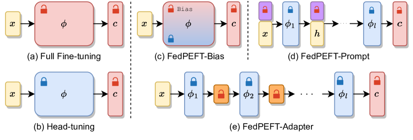
Figure 2: Methods to fine-tune the pre-trained model, where $x$ means the input, $\phi$ means the backbone, $\phi_{i}$ means the $i$-th layer of $\phi$ with $l$ layers in total, $c$ means the classification head, and $h$ means the hidden states. (a) Fully fine-tune the entire model. (b) Only tune the model head. (c) Only tune the bias term and the model head. (d) Concatenate prompts to the input and hidden states in each layer, and only tune the prompts and the model head. The purple rectangles denote the tunable prompts. (e) Add an adapter to each layer of the backbone, and only tune the adapters and the model head. The orange rectangles denote the tunable adapters.

3.2 FedPEFT

In conventional federated learning, updates for the entire model need to be repeatedly sent to and from the server, resulting in significant communication costs, especially when larger, more capable modern neural network architectures are employed. To reduce this heavy burden, we deploy parameter-efficient fine-tuning methods to adapt pre-trained models to the local clients rather than fully fine-tuning all parameters, which is described in Algorithm 1. In the FedPEFT framework, illustrated in Figure 1, only a small amount of parameters in the local model will be downloaded, trained, and uploaded in each communication round. For instance, FedPEFT reduces the size of communication each round from 328MB/Client to 0.68MB/Client when using a pre-trained ViT-Base as the backbone.

To implement FedPEFT, we provide a canonical baseline approach (Head-tuning) and three prototypes leveraging different parameter-efficient fine-tuning methods (Bias, Adapter, and Prompt), which are detailed in the following.

To reduce the number of trainable parameters, one intuitive method, Head-tuning, is to freeze the backbone $\phi$ and only train the head $c$. This method is historically the most common fine-tuning procedure, and therefore we use it as a baseline for FedPEFT. However, the adaptation ability of this method is limited, as no adjustment is made to the network representation prior to the final output head. This can be problematic in the presence of a more intense domain shift. Therefore, we consider the following approaches as primary prototypes for FedPEFT:

FedPEFT-Bias. Bias-tuning [3] aims to adapt the pre-trained backbone $\phi$ with only fine-tuning a specific group of parameters, the bias term. In this way, the backbone can be trained with moderate adjustments to prevent damaging the upstream representation.

FedPEFT-Adapter. Instead of directly tuning existing parameters in the backbone like Bias-tuning, Adapter-tuning [33] adds a few parameters called adapters inside the backbone $\phi$ instead. Usually, adapters will be deployed in each layer of the backbone to perform transformations on different levels of the pre-trained feature while the backbone stays frozen.

FedPEFT-Prompt. Prompt-tuning [19] takes a slightly different approach from the other fine-tuning methods. Specifically, it concatenates trainable parameters, called prompt embeddings, to the input embedding and hidden states in each layer.

We illustrate the differences between all baseline and prototype methods in Figure 2. We also provide the algorithm pseudo-code for each prototype in the Supplementary.

Table 1: Communication analysis. The communication cost is computed with 4B/parameter. The averaged final accuracy, i.e., $t=T=50$, and the standard deviation of three different random seeds are reported for each data set. The first section shows the change in accuracy when decreasing the participating-client number. The gray numbers indicate the baseline performance with no decrease in the participating-client number. The second section shows the change in accuracy when we reward the low communication cost of head-tuning by increasing the number of participating clients. The third section shows the accuracy when we fully fine-tune a lightweight model, ShuffleNet V2 $0.5\times$ [28]. The fourth section shows the performance of each prototype of FedPEFT.

Model	Method	# Tuned Params $\times$ Clients	Comm. Cost	Resisc45	CIFAR-100	PCam
ViT-B	Full Fine-tuning	85.88M $\times$ 8	2.56GB	91.49$\pm$0.82	91.73$\pm$0.43	85.41$\pm$2.41
ViT-B	Full Fine-tuning	85.88M $\times$ 4	1.28GB	92.13$\pm$0.87	89.69$\pm$0.30	81.93$\pm$3.54
ViT-B	Full Fine-tuning	85.88M $\times$ 2	656MB	87.68$\pm$1.32	87.03$\pm$0.18	82.20$\pm$1.22
ViT-B	Full Fine-tuning	85.88M $\times$ 1	328MB	73.38$\pm$1.95	74.79$\pm$0.77	80.18$\pm$1.83
ViT-B	Head-tuning	0.08M $\times$ 8	2.44MB	77.30$\pm$1.03	72.45$\pm$0.08	74.82$\pm$2.40
ViT-B	Head-tuning	0.08M $\times$ 64	19.53MB	83.58$\pm$0.45	75.45$\pm$0.16	77.82$\pm$0.37
ShuffleNet	Full Fine-tuning	0.44M $\times$ 8	13.43MB	63.52$\pm$0.50	49.81$\pm$1.94	76.52$\pm$3.35
ViT-B	FedPEFT-Bias	0.18M $\times$ 8	5.49MB	89.04$\pm$0.80	90.79$\pm$0.25	85.51$\pm$0.66
ViT-B	FedPEFT-Adapter	0.23M$\times$ 8	7.02MB	87.20$\pm$0.78	87.74$\pm$0.55	78.67$\pm$1.85
ViT-B	FedPEFT-Prompt	0.17M$\times$ 8	5.19MB	83.35$\pm$0.76	89.78$\pm$0.84	86.50$\pm$0.85

4 Experiments

The capability of full fine-tuning in terms of accuracy has been illustrated in recent work [31, 7], thus we regard it as a competitive baseline for FedPEFT. To verify the performance of FedPEFT comprehensively, we evaluate the server accuracy with each method from three perspectives and aim to answer the following questions:

Communication Analysis: When faced with a limited communication budget, there are several conventional solutions to reduce costs, e.g., sampling fewer clients each round or using a lightweight model. Can FedPEFT outperform other solutions in terms of communication cost and accuracy? (RQ1)

Capability Analysis: When the communication budget is amply sufficient for all approaches, we want to evaluate the trade-off of training fewer parameters with FedPEFT. Can FedPEFT outperform full fine-tuning and training from scratch within various federated learning settings and increasing levels of downstream domain gap? (RQ2)

Robustness Analysis: In a lot of application scenarios, there will be additional challenges for FL, such as privacy-preserving requirements (i.e., differential privacy) and data scarcity (i.e., very small amount of data on each client). We want to evaluate the robustness of each method under such scenarios. Can FedPEFT outperform full fine-tuning in terms of robustness? (RQ3)

4.1 Experiments details

Dataset. For our study, we focus on computer vision (CV) applications as our testbed. Therefore, we employ ImageNet-21K [34] as the pre-training dataset, which is a primary dataset for pre-training models in CV. Then we select three datasets for the downstream tasks that have increasing degrees of domain gap compared to ImageNet-21k, and we visualize and quantify the domain gap in Section 6.1: Resisc45 [8], CIFAR-100 [23] and PCam [41]. Resisc45 is a remote sensing image dataset containing 18,900 training samples and 6,300 testing samples for 45 scene classes, which has a small domain gap with ImangeNet-21K. CIFAR-100 contains 50,000 training samples and 10,000 testing samples for 100 classes of nature objects (e.g., sunflowers, buses), which has a medium domain gap. PCam is a medical dataset containing 32,768 colored images extracted from histopathologic scans of lymph node sections, which has a much larger domain gap. Each image is annotated with a binary label indicating the presence of metastatic tissue. We sample 20,000 images from the original train set for training and use the entire test set for evaluation. We use the official splitting for CIFAR-100 and PCam and a public splitting from AiTLAS [10] for Resisc45.

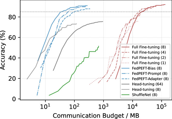
Figure 3: Server accuracy given the total communication budget. The communication cost is computed with 4B/parameter, and the max number of communication rounds is 50. The number in the bracket next to the method indicates the number of participating clients $m$. The transparency of the line indicates the ratio between $m$ and total client number $N=64$. The horizontal dashed line shows a target accuracy of $85\%$

Experimental Setting. Our default experimental setting is to split the dataset across $N=64$ clients and sample $M=8$ clients each round. The global aggregation will be performed after $E=10$ local epochs. A total of $T=50$ rounds of communication will be performed. To simulate heterogeneous data, we partition samples in each class to all clients following a Dirichlet distribution, as common in the literature [30, 1, 25], with $\alpha=0.1$ for CIFAR-100 and Resisc45 and $\alpha=0.5$ for PCam based on the class number. Any modifications to this setting in subsequent experiments will be clearly noted.

Implementation Detail. We choose ViT-B [11] with image size 224 and patch size 16 as our backbone. The backbone is pre-trained on ImageNet-21K [34], as available in the timm library [45]. The images for the downstream datasets are resized to $224\times 224$. Images from CIFAR-100 are augmented by random cropping with a padding of $4$ and random horizontal flipping, and Resisc45 and PCam are augmented only with random horizontal flipping. We perform the experiments on 8 Nvidia RTX A5000 GPUs with a batch size of $64$. All reported numbers are run multiple times and averaged. More details about hyperparameter searching can be found in the Supplementary. The base hyperparameters for each method are described below.

• Full fine-tuning: We use SGD [35] optimizer with learning rate $0.001$ and weight decay $0.0001$.

• Head-tuning: We use one linear layer as the classification head and use the SGD optimizer with learning rate $0.005$ and weight decay $0.0001$.

• FedPEFT-Bias: There is no additional hyperparameter for Bias. We use SGD optimizer with learning rate $0.01$ and weight decay $0.0001$.

• FedPEFT-Adapter: We use a Bottleneck Adapter with residual connections as the adapter. We insert the adapter to each layer of the backbone after the feed-forward block following [33] with a reduction factor of $8$ and the GELU as the activation function. We use SGD optimizer with learning rate $0.005$ and weight decay $0.0001$.

• FedPEFT-Prompt: We follow the design of VPT-Deep [19], and use a prompt length as $10$ to prepend prompt tokens to the input and the hidden embedding in each layer. We use SGD optimizer with learning rate $0.01$ and weight decay $0.0001$.

5 Communication Analysis

To verify the effectiveness of FedPEFT and answer the first research question (RQ1, Section 4), we compare it with three baselines while monitoring the communication budget: a) Full fine-tuning of our default model (ViT-B). We vary the number of participating clients to show different levels of communication requirements. b) Head-tuning. The communication cost of head-tuning is naturally lower than other methods, so we increase the participating clients to make it a stronger baseline. c) Fully fine-tune a light-weighted model (ShuffleNet V2 0.5$\times$ [28]) with a similar parameter scale.

As demonstrated in Table 1, all FedPEFT methods achieve better results in many cases compared with other approaches, even with significantly fewer communicated parameters. We find that full fine-tuning needs several orders of magnitude of communication to achieve a comparable result with FedPEFT. For instance, it needs at least 187$\times$ and 477$\times$ more parameters to reach and outperform FedPEFT on CIFAR-100. Interestingly, full fine-tuning performs well on Resisc45 where the domain gap is smaller, even when the participating-client number is low. However, when the domain gap increases, more participating clients will be needed to outperform FedPEFT, and finally it fails to outperform FedPEFT even without reducing the participating-client number on PCam where a large domain gap exists. Meanwhile, head-tuning lags behind most other approaches, but the performance is stable with different levels of domain gap, while the ShuffleNet model only achieves $71\%$, $55\%$, and $89\%$ of accuracy on Resisc45, CIFAR-100, and PCam with 2.4$\times$ the communication cost compared with FedPEFT-Bias. Besides, the standard deviation of FedPEFT is lower than most other solutions, especially when the domain gap is large, showing the stability of FedPEFT.

In Figure 3, we also report the server accuracy that can be achieved for each method given the communication budgets using CIFAR-100 as an example. The plots for the remaining datasets can be found in the Supplementary. The communication cost per communication round for full fine-tuning is even higher than the total communication cost for FedPEFT to converge to similar final server accuracy. Meanwhile, all FedPEFT prototypes only require megabytes level communication, while full fine-tuning requires gigabytes level communication to reach a given target accuracy (e.g., 85% in Fig. 3), showing the efficiency of FedPEFT. For the inter-prototype comparison, FedPEFT-Bias stands out for its highest efficiency. We provide further discussions on the performance of each prototype in Section 6.

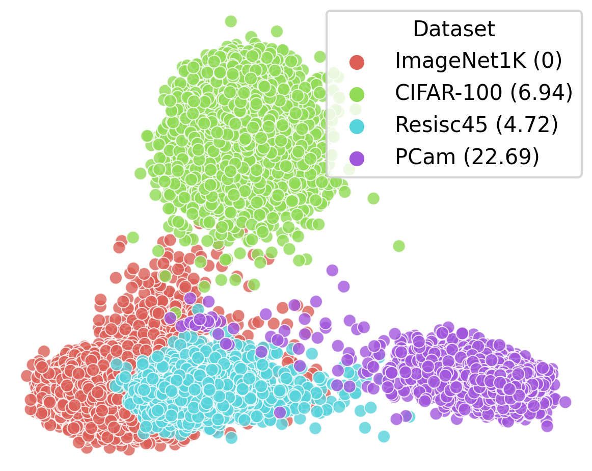
(a) Extracted feature. The number in the bracket is the domain gap to the pre-training dataset.

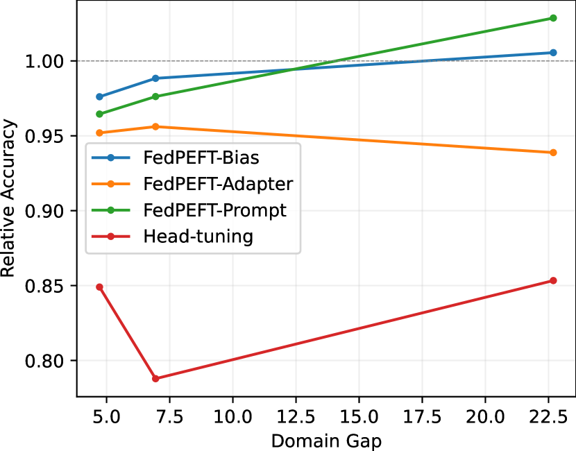
(b) Relative accuracy of each method compared with full fine-tuning with different domain gaps.

Figure 4: Visualization and analysis of domain gap. (a) We apply Linear Discriminant Analysis (LDA) to the extracted feature from the pre-trained backbone to visualize and quantify the domain gap. (b) We plot the performance (relative accuracy) of each PEFT method compared against full fine-tuning. The gray dashed line indicates the performance of full fine-tuning (i.e., reference), and the three points in each line are the relative server accuracy on Resisc45, CIFAR-100, and PCam respectively.

6 Capability Analysis

To study and understand our second research question (RQ2, Section 4), we analyze the impact of the domain gap between the model pre-training dataset and the dataset for FL (Section 6.1) and systemically perform experiments on CIFAR-100 across different federated learning scenarios by varying client status and data distribution (Section 6.2).

6.1 Capability with Domain Gap

Domain gap is a realistic concern when deploying pre-trained models for downstream tasks. To visualize and quantify the domain gap between each downstream dataset and the pre-training dataset, we adapt Linear Discriminant Analysis (LDA) for all extracted features for the test samples in each dataset from the pre-trained backbone. We compute the center of each dataset and then compute the distance to the center of the pre-training dataset as the quantifying result of the domain gap, as shown in Figure 4(a).

In Figure 4(b), we present the performance of all approaches with an increasing degree of domain gap compared to the ImageNet-21k pre-training dataset. Interestingly, full fine-tuning falls further behind as the data domain gap widens in the PCam scenario, largely unable to keep up with FedPEFT despite requiring a massive communication budget. This phenomenon when a pre-trained model meets out-of-domain data has been studied under centralized settings [37]. It was found that the pre-trained upstream representations are still meaningful even with a domain gap. Therefore, fully fine-tuning the backbone with out-of-domain data can damage the high-level semantics inside these upstream representations due to overfitting, especially when the data size is small. This is particularly relevant in FL, where overfitting and subsequent client drift [40, 30, 21] are prone to occur.

On the opposite end of the spectrum, by not fine-tuning the backbone at all, head-tuning maintains similar accuracy despite the domain gap. This shows the robustness of the pre-trained high-level semantics across domains, supporting the conclusion that there is meaningful high-level semantics inside of the upstream representations.

Still, the tight restriction on head-tuning is perhaps a bit too far, as the accuracy on both datasets is still low overall. Between the two extremes of head-tuning and full fine-tuning, FedPEFT approaches may be able to suitably adapt the upstream representations without excessively damaging them. Specifically, FedPEFT-Bias operates with parameter-level control for each parameter pair containing weight and bias terms. The representation can then preserve the high-level semantics by freezing the weight term (maintaining the direction in the feature space) and still adapting via the bias term (shifting in the feature space). FedPEFT-Adapter and FedPEFT-Prompt have slightly different mechanisms (layer-level), controlling the backbone by transforming the intermediate hidden representations via adapters and prompts. However, the capability to handle the domain gap of FedPEFT-Prompt is stronger than FedPEFT-Adapter. Of these approaches, FedPEFT-Prompt is the most stable under the domain gap, surpassing full fine-tuning by  1.1% on PCam. Overall, we hypothesize that more fine-tuning freedom will be better when the domain gap is minor, but moderate fine-tuning is needed to maintain, as well as control, the high-level semantics when the domain gap is large.

Table 2: Capability analysis among different federated learning settings on CIFAR-100. Bold-style shows the best performance among all methods or among prototypes in FedFEFT.

Client	Method	# Tuned Params	Homogeneous	Heterogeneous
$\begin{aligned} &N=16\\ &M=16\end{aligned}$	Scratch	85.88M	38.44	35.72
	Full Fine-tuning	85.88M	93.70	93.50
	Head-tuning	0.08M	78.11	77.59
	FedPEFT-Bias	0.18M	91.89	90.25
	FedPEFT-Adapter	0.23M	90.21	88.77
	FedPEFT-Prompt	0.17M	92.09	90.37
$\begin{aligned} &N=16\\ &M=2\end{aligned}$	Full Fine-tuning	85.88M	93.32	87.01
	Head-tuning	0.08M	76.65	62.80
	FedPEFT-Bias	0.18M	91.35	86.18
	FedPEFT-Adapter	0.23M	89.48	80.08
	FedPEFT-Prompt	0.17M	91.60	85.54
$\begin{aligned} &N=64\\ &M=64\end{aligned}$	Full Fine-tuning	85.88M	93.66	92.81
	Head-tuning	0.08M	78.45	75.51
	FedPEFT-Bias	0.18M	92.71	91.71
	FedPEFT-Adapter	0.23M	90.50	89.26
	FedPEFT-Prompt	0.17M	91.87	90.96
$\begin{aligned} &N=64\\ &M=8\end{aligned}$	Full Fine-tuning	85.88M	93.50	92.09
	Head-tuning	0.08M	77.59	72.55
	FedPEFT-Bias	0.18M	92.49	91.02
	FedPEFT-Adapter	0.23M	90.39	88.05
	FedPEFT-Prompt	0.17M	92.00	89.90

Table 3: Robustness analysis for privacy-preserving. The red number indicates the performance difference when DP is applied.

Method	w/o DP	w/ DP
Full Fine-tuning	92.09	77.61 (-14.48)
Head-tuning	72.55	62.20 (-10.35)
FedPEFT-Bias	91.02	84.98 (-6.04)
FedPEFT-Adapter	88.05	79.05 (-9.00)
FedPEFT-Prompt	89.90	78.35 (-11.55)

6.2 Capability with Different FL Settings

In application scenarios, the setting of federated learning can vary substantially. It is important to show the capability to maintain high performance in diverse settings. In Table 2, we present results for all approaches with different client availability ratios and data distributions and draw the following conclusions from the experiments:

First, we see that fine-tuning the pre-trained model shows a significant improvement over training from scratch, especially in heterogeneous scenarios. This finding is in agreement with other very recent works [7, 31], which note the stabilization effect of pre-trained initialization in federated optimization. When only fine-tuning the head, the performance is still much better than training the entire model from scratch (Scratch) but remains low in comparison to other methods across all settings. We again find that head-tuning simply lacks adaptation ability, holding too closely to the upstream representation.

On the other hand, we find that FedPEFT achieves comparable results to full fine-tuning with less than 0.3% of the trainable parameters. This ability to maintain accuracy performance in various scenarios is crucial for FL, as oftentimes, the exact setting and distributions are not known ahead of time. With this in mind, we further investigate the viability of FedPEFT as a practical FL framework in some more extreme situations in Section 7.

7 Robustness Analysis

In this section, we further investigate our third research question (RQ3) in two critical FL scenarios. CIFAR-100 is used for the experiments.

Differential Privacy. A fundamental property of federated learning is privacy protection. However, various works [18, 16] have demonstrated how the client data can be reconstructed from the raw gradient updates received by the server in some scenarios. To protect client data privacy from such attacks, differential privacy (DP) [20, 5, 12, 13] has become standard practice. Therefore, we first study FedPEFT and other baselines under DP.

Table 4: Robustness analysis for data scarcity. $K$ indicates the total sample number of all clients.

Method	$K=1000$	$K=1500$	$K=2000$
Full Fine-tuning	66.52	67.47	77.67
Head-tuning	52.13	56.52	60.15
FedPEFT-Bias	76.40	81.14	83.83
FedPEFT-Adapter	71.34	76.91	79.22
FedPEFT-Prompt	63.77	71.94	76.89

To integrate DP, we apply a Gaussian mechanism within the local optimization of each iteration [13] with $\varepsilon=5$ and $\delta=0.001$. We maintain the remaining FL settings as described in Section 4.1, and show the results in Table 3. Interestingly, when comparing all methods, full fine-tuning experiences the sharpest drop with DP. This causes its accuracy to fall lower than all the FedPEFT prototypes. To understand this effect, we note that DP applies noise to all trainable parameter gradients. Full fine-tuning, therefore, requires such noise on all model parameters, resulting in a more pronounced negative effect on final performance. On the other hand, the other fine-tuning methods maintain some part of the backbone frozen and have significantly fewer trainable parameters on which adding noise is necessary, limiting the performance drop. Overall, FedPEFT allows for stronger accuracy in DP-enabled federated systems than even full fine-tuning while still maintaining extremely low communication needs.

Data Scarcity. We explore another common yet challenging robustness condition in FL; that is when very little data is available on individual clients. Such data scarcity scenarios are even a tricky problem in centralized training. For example, [44] show that fewer training data will incur damage to the pre-trained representation due to overfitting. In our evaluation for FL, we reduce the total sample number $K$ to $1000$, $1500$, and $2000$. As shown in Table 4, we find that FedPEFT outperforms full fine-tuning and head-tuning under such low-data scenarios, further revealing its capability to appropriately adapt pre-trained representations to the FL task at hand.

Table 5: Ablation study on network backbone and pre-training dataset. 1K and 21K mean pre-trained on ImageNet1K and ImageNet21K respectively. The server accuracy (acc) on CIFAR-100 is reported.

Method	Backbone	Pre-training	Server Acc (%)
Full Fine-tuning	ViT-B	Supervised (21K)	92.09
	ViT-B	Supervised (1K)	92.09
	ViT-S	Supervised (21K)	89.33
	ViT-B	DINO (1K)	85.62
Head-tuning	ViT-B	Supervised (21K)	72.55
	ViT-B	Supervised (1K)	80.78
	ViT-S	Supervised (21K)	74.40
	ViT-B	DINO (1K)	77.17
FedPEFT-Bias	ViT-B	ImageNet-21K	91.02
	ViT-B	Supervised (1K)	90.73
	ViT-S	Supervised (21K)	88.40
	ViT-B	DINO (1K)	85.34
FedPEFT-Adapter	ViT-B	ImageNet-21K	87.99
	ViT-B	Supervised (1K)	88.69
	ViT-S	Supervised (21K)	84.15
	ViT-B	DINO (1K)	83.29
FedPEFT-Prompt	ViT-B	ImageNet-21K	89.63
	ViT-B	Supervised (1K)	89.29
	ViT-S	Supervised (21K)	87.39
	ViT-B	DINO (1K)	84.25

8 Pre-training Ablations

In the experiments above, we maintain a consistent backbone (ViT-B). However, since model size requirements of different federated systems may vary, we further investigate the use of ViT-S with FedPEFT and all baselines. Additionally, we study the effect of pre-training dataset size and paradigm on the final performance of all approaches. CIFAR-100 is used for the experiments, and the results are presented in Table 5.

Impact of Model Size. We replace ViT-B with a smaller version, ViT-S. As expected, most methods experience a slight performance drop. Nonetheless, FedPEFT methods maintain strong performance even with smaller models. Surprisingly, the performance of head-tuning is not damaged by reducing the model size but actually increases slightly. We interpret it as due to the fixed representation of head-tuning. Representations from a pre-trained model can have similar semantics whatever the model size, thus the performance of head-tuning is stable.

Impact of Pre-training Dataset. We also evaluate the performance when a backbone is trained from ImageNet-21K and ImageNet-1K [36]. Interestingly, the performance stays relatively consistent, with Head-tuning and FedPEFT-Adapter achieving higher accuracy with the ImageNet-1K models. This phenomenon indicates that the performance of fine-tuning is not always proportional to the data size, but overall FedPEFT performance is consistent with different scales of the pre-training dataset.

Impact of Pre-training Paradigm. Additionally, we evaluate one self-supervised pre-trained backbone: DINO [4]. FedPEFT still achieves comparable results with full fine-tuning and outperforms Head-tuning, showing the robustness of FedPEFT.

9 Conclusion

In this paper, we introduce FedPEFT, a new federated learning framework leveraging strong pre-trained models and massively reducing communication costs. We integrate three effective prototypes within the FedPEFT framework: Bias, Adapter, and Prompt. With a thorough empirical study, we then evaluate FedFEFT and other baselines in three key areas: communication, capability, and robustness. We find FedPEFT to be a promising approach for practical FL systems, capable of handling many of the harsh conditions in FL while alleviating the critical communication bottleneck. As a general framework, FedPEFT can also be leveraged in application domains other than computer vision, which we leave for future work. We hope this work can inspire new perspectives in federated learning through the combined innovation of strong pre-trained models and parameter-efficient fine-tuning methodologies.

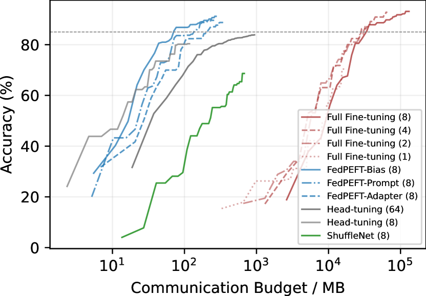
(a) Resisc45

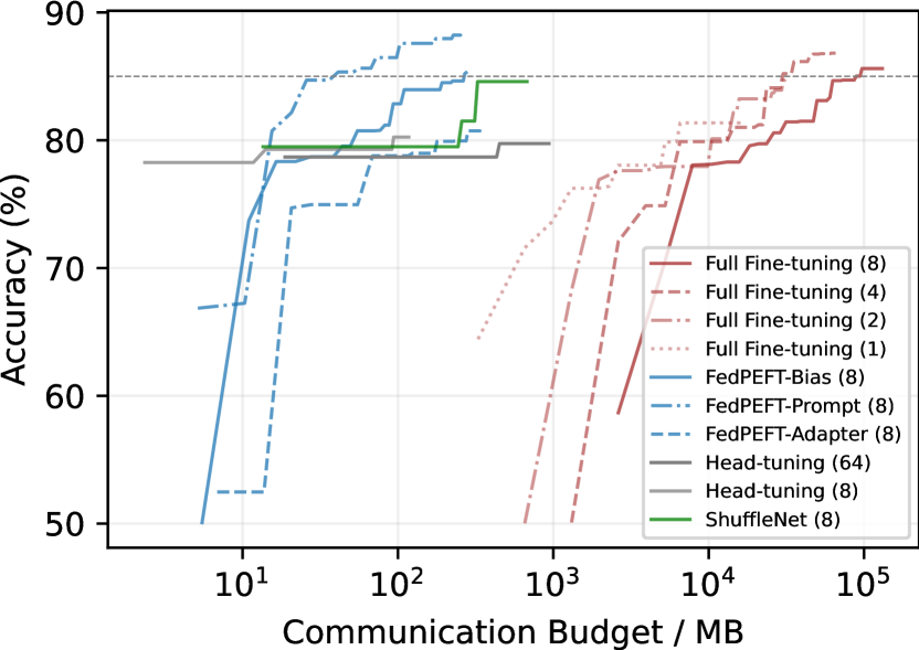
(b) PCam

Figure 5: Server accuracy given the total communication budget. The communication cost is computed with 4B/parameter, and the max number of communication rounds is 50. The number in the bracket next to the method indicates the number of participating clients $m$. The transparency of the line indicates the ratio between $m$ and total client number $N=64$. The horizontal dashed line shows a target accuracy of $85\%$

Appendix A Overview

Here is the outline of the supplementary:

• Appendix B: Implementation details of all the experiments, including pseudocode, random states, data partitioning and hyperparameters.

• Appendix C: Supplemental experiment results on Resisc45 and PCam.

• Appendix D: Visualization and analysis of FedPEFT.

• Appendix E: Broader impact and limitation of FedPEFT.

Appendix B Implement Details

B.1 Pseudocode for Each Prototype

We provide detailed Pytorch-style pseudocode for each prototype in Algorithms 2, 3 and 4. Furthermore, our full code will be made publicly available upon acceptance.

Table 6: Optimal learning rate for each setting. FFT: Full Fine-tuning, HT: Head-tuning. Homo: homogeneous data, $\alpha$: parameter for the Dirichlet distribution.

Setting	Dataset	FFT	HT	Bias	Adapter	Prompt
$N=64,M=8,\alpha=0.1$	Resisc45	5e-4	1e-2	5e-3	5e-3	1e-2
$N=64,M=8,\alpha=0.1$	CIFAR-100	5e-4	1e-2	1e-2	5e-3	1e-2
$N=64,M=8,\alpha=0.5$	PCam	5e-4	1e-2	1e-2	5e-3	1e-2
$N=64,M=8,$ homo	Resisc45	1e-3	5e-3	5e-3	5e-3	1e-2
$N=64,M=64,\alpha=0.1$	Resisc45	1e-3	5e-3	5e-3	5e-3	1e-2
$N=64,M=64,$ homo	Resisc45	1e-3	5e-3	5e-3	5e-3	1e-2
$N=16,M=16,\alpha=0.1$	Resisc45	1e-3	5e-3	5e-3	5e-3	1e-2
$N=16,M=16,$ homo	Resisc45	1e-3	5e-3	5e-3	5e-3	1e-2
$N=16,M=2,\alpha=0.1$	Resisc45	1e-3	5e-3	5e-3	5e-3	1e-2
$N=16,M=2,$ homo	Resisc45	1e-3	5e-3	5e-3	5e-3	1e-2
$N=64,M=8,$ homo	CIFAR-100	1e-3	5e-3	1e-2	5e-3	1e-2
$N=64,M=64,\alpha=0.1$	CIFAR-100	1e-3	5e-3	1e-2	5e-3	1e-2
$N=64,M=64,$ homo	CIFAR-100	1e-3	5e-3	1e-2	5e-3	1e-2
$N=16,M=16,\alpha=0.1$	CIFAR-100	1e-3	5e-3	1e-2	5e-3	1e-2
$N=16,M=16,$ homo	CIFAR-100	1e-3	5e-3	1e-2	5e-3	1e-2
$N=16,M=2,\alpha=0.1$	CIFAR-100	1e-3	5e-3	1e-2	5e-3	1e-2
$N=16,M=2,$ homo	CIFAR-100	1e-3	5e-3	1e-2	5e-3	1e-2
$N=64,M=8,$ homo	PCam	1e-3	5e-3	1e-2	5e-3	1e-2
$N=64,M=64,\alpha=0.1$	PCam	1e-3	5e-3	1e-2	5e-3	1e-2
$N=64,M=64,$ homo	PCam	1e-3	5e-3	1e-2	5e-3	1e-2
$N=16,M=16,\alpha=0.1$	PCam	1e-3	5e-3	1e-2	5e-3	1e-2
$N=16,M=16,$ homo	PCam	1e-3	5e-3	1e-2	5e-3	1e-2
$N=16,M=2,\alpha=0.1$	PCam	1e-3	5e-3	1e-2	5e-3	1e-2
$N=16,M=2,$ homo	PCam	1e-3	5e-3	1e-2	5e-3	1e-2
$N=64,M=8,\alpha=0.1,$ DP	CIFAR-100	1e-4	5e-4	1e-3	5e-4	3e-4
$N=64,M=8,\alpha=0.1,K=1000$	CIFAR-100	1e-3	5e-3	1e-2	1e-3	1e-2
$N=64,M=8,\alpha=0.1,K=1500$	CIFAR-100	1e-3	5e-3	1e-2	5e-3	1e-2
$N=64,M=8,\alpha=0.1,K=2000$	CIFAR-100	1e-3	5e-3	1e-2	5e-3	1e-2

B.2 Random States

We choose three different random seeds, 1, 42, and 3407, for our main results. For further analysis, we fix the random seed as 1.

B.3 Data Partitioning

We perform a common data partitioning as in other previous work [30, 1, 25]. We partition samples in each class to all clients following a Dirichlet distribution, with $\alpha=0.1$ for CIFAR-100 and Resisc45 and $\alpha=0.5$ for PCam based on the class number. We visualize the data distribution as shown in Figure 6.

B.4 Hyperparameter Searching

The most crucial hyperparameter in our experiments is the learning rate. We search this hyperparameter with several options in a grid-search-like fashion. The initial options for learning rate are $\{1e-4,5e-4.1e-3,5e-3,1e-2,5e-2\}$. The specific optimal learning rate for each setting is shown in Table 6. The optimal learning rates for other comparison methods are listed here:

• ShuffleNet in Resisc45: 5e-2

• ShuffleNet in CIFAR-100: 5e-2

• ShuffleNet in PCam: 1e-1

• Training from Scratch with homogeneous data: 1e-2

• Training from Scratch with heterogeneous data: 1e-2

Appendix C Supplemental Experiment Results

C.1 Communication Analysis for Resisc45 and PCam

Figures 5(a) and 5(b) show the communication analysis on Resisc45 and PCam, complementary to the main result in Section 5. The conclusion on these two datasets is consistent with our results and analysis in the main paper.

C.2 Different FL Settings for Resisc45 and PCam

Tables 7 and 8 show the capability analysis on Resisc45 and PCam as a supplementary for the main result in Section 6. As expected, when the domain gap is smaller, i.e., Resisc45, the performance of Full Fine-tuning is slightly better than FedPEFT, benefiting from the highest level of fine-tuning. Meanwhile, in the presence of more domain gaps with PCam, pre-trained representations are problematic for the target domain, leading to a performance lower than training from scratch for Head-tuning. Therefore, fine-tuning beyond the head is necessary and helpful when facing domain gaps. The performance of Full Fine-tuning and FedPEFT is better than Head-tuning in such cases, especially with more participating clients. Among these two fine-tuning strategies, FedPEFT outperforms full fine-tuning in almost all FL settings when facing out-of-domain data, showing the robustness of FedPEFT and the potential to be applied to various FL scenarios.

Table 7: Capability analysis among different federated learning settings on Resisc45. Bold-style shows the best performance among all methods or among prototypes in FedFEFT.

Client	Method	# Tuned Params	Homogeneous	Heterogeneous
$\begin{aligned} &N=16\\ &M=16\end{aligned}$	Scratch	85.88M	54.86	49.35
	Full Fine-tuning	85.88M	94.81	93.52
	Head-tuning	0.08M	88.11	85.02
	FedPEFT-Bias	0.18M	93.48	91.83
	FedPEFT-Adapter	0.23M	93.06	90.89
	FedPEFT-Prompt	0.17M	92.78	91.57
$\begin{aligned} &N=16\\ &M=2\end{aligned}$	Full Fine-tuning	85.88M	95.60	90.94
	Head-tuning	0.08M	87.95	63.71
	FedPEFT-Bias	0.18M	93.67	86.59
	FedPEFT-Adapter	0.23M	92.44	81.92
	FedPEFT-Prompt	0.17M	92.79	86.02
$\begin{aligned} &N=64\\ &M=64\end{aligned}$	Full Fine-tuning	85.88M	93.67	92.91
	Head-tuning	0.08M	87.41	83.87
	FedPEFT-Bias	0.18M	93.05	91.30
	FedPEFT-Adapter	0.23M	92.13	89.68
	FedPEFT-Prompt	0.17M	92.19	90.81
$\begin{aligned} &N=64\\ &M=8\end{aligned}$	Full Fine-tuning	85.88M	94.02	92.40
	Head-tuning	0.08M	87.46	78.41
	FedPEFT-Bias	0.18M	92.69	90.49
	FedPEFT-Adapter	0.23M	91.92	87.97
	FedPEFT-Prompt	0.17M	91.91	88.29

Table 8: Capability analysis among different federated learning settings on PCam. Bold-style shows the best performance among all methods or among prototypes in FedFEFT.

Client	Method	# Tuned Params	Homogeneous	Heterogeneous
$\begin{aligned} &N=16\\ &M=16\end{aligned}$	Scratch	85.88M	77.24	77.16
	Full Fine-tuning	85.88M	84.16	85.69
	Head-tuning	0.08M	76.31	75.68
	FedPEFT-Bias	0.18M	86.68	86.74
	FedPEFT-Adapter	0.23M	78.18	82.66
	FedPEFT-Prompt	0.17M	85.76	84.24
$\begin{aligned} &N=16\\ &M=2\end{aligned}$	Full Fine-tuning	85.88M	80.96	84.01
	Head-tuning	0.08M	74.57	50.11
	FedPEFT-Bias	0.18M	81.45	84.60
	FedPEFT-Adapter	0.23M	77.87	79.98
	FedPEFT-Prompt	0.17M	79.50	72.18
$\begin{aligned} &N=64\\ &M=64\end{aligned}$	Full Fine-tuning	85.88M	84.05	86.54
	Head-tuning	0.08M	76.15	78.24
	FedPEFT-Bias	0.18M	84.22	85.46
	FedPEFT-Adapter	0.23M	79.41	80.58
	FedPEFT-Prompt	0.17M	82.88	85.75
$\begin{aligned} &N=64\\ &M=8\end{aligned}$	Full Fine-tuning	85.88M	83.69	84.82
	Head-tuning	0.08M	73.50	72.38
	FedPEFT-Bias	0.18M	83.05	85.29
	FedPEFT-Adapter	0.23M	80.79	79.63
	FedPEFT-Prompt	0.17M	85.39	87.25

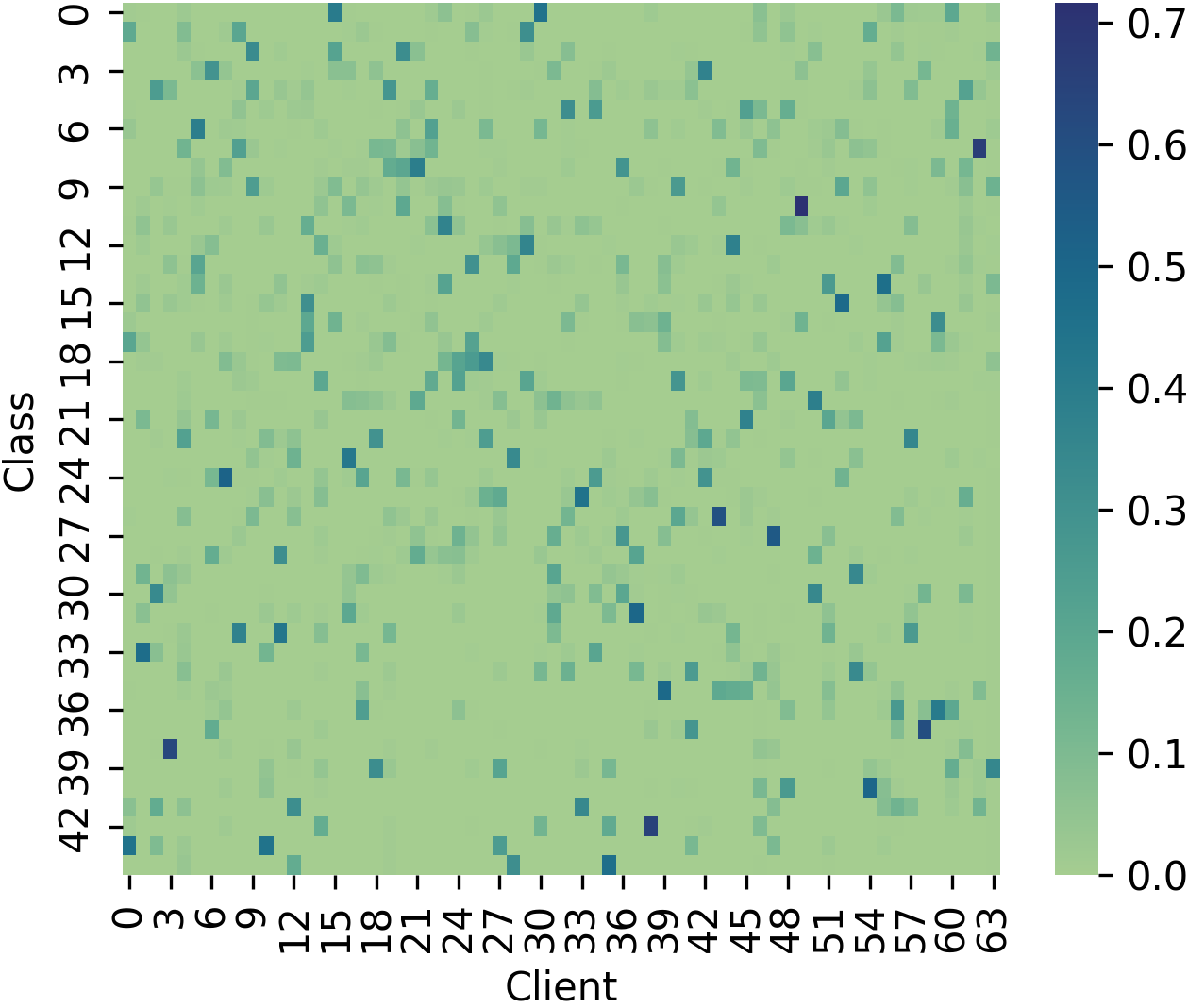
(a) Resisc45, $\alpha=0.1$

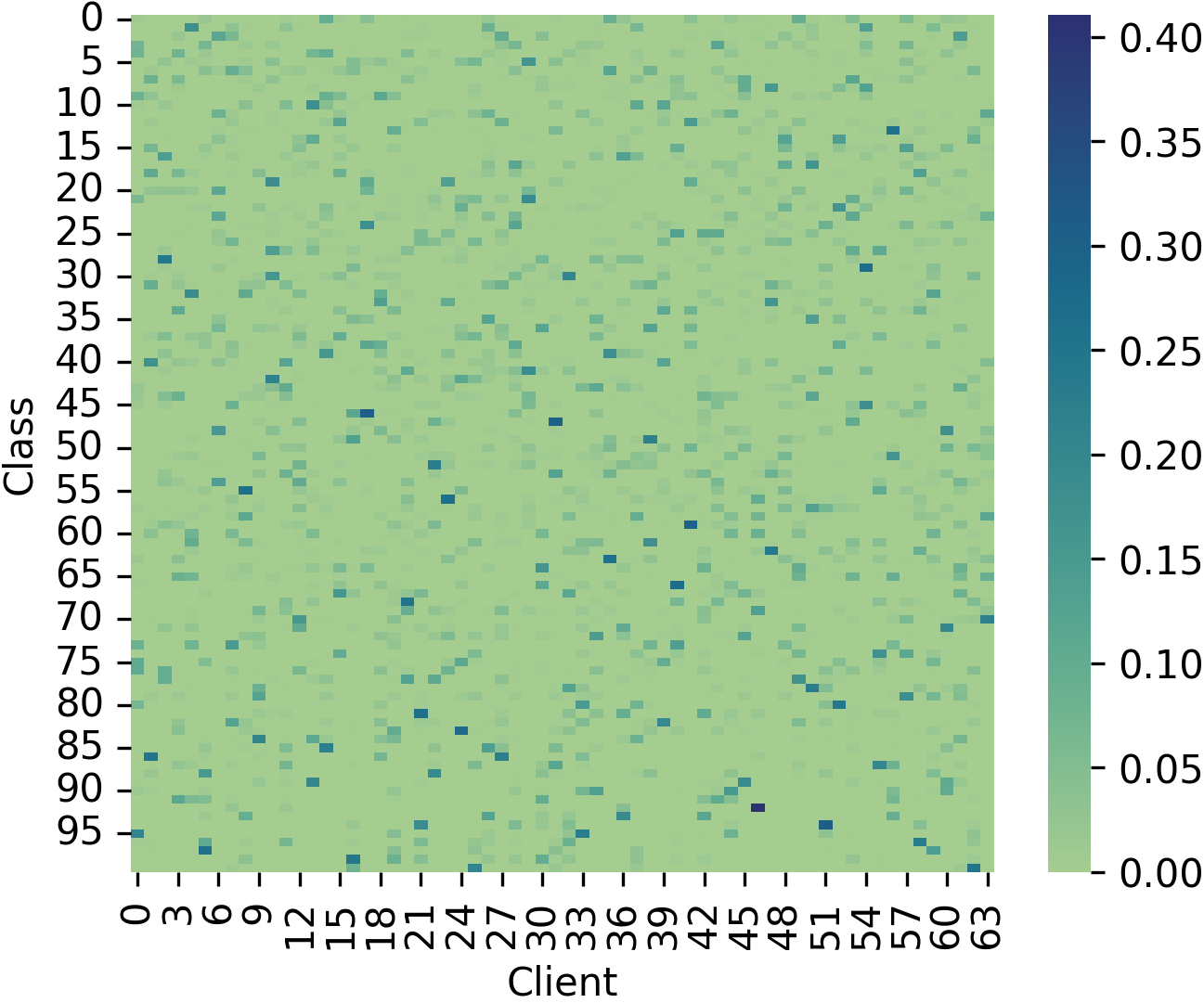
(b) CIFAR-100, $\alpha=0.1$

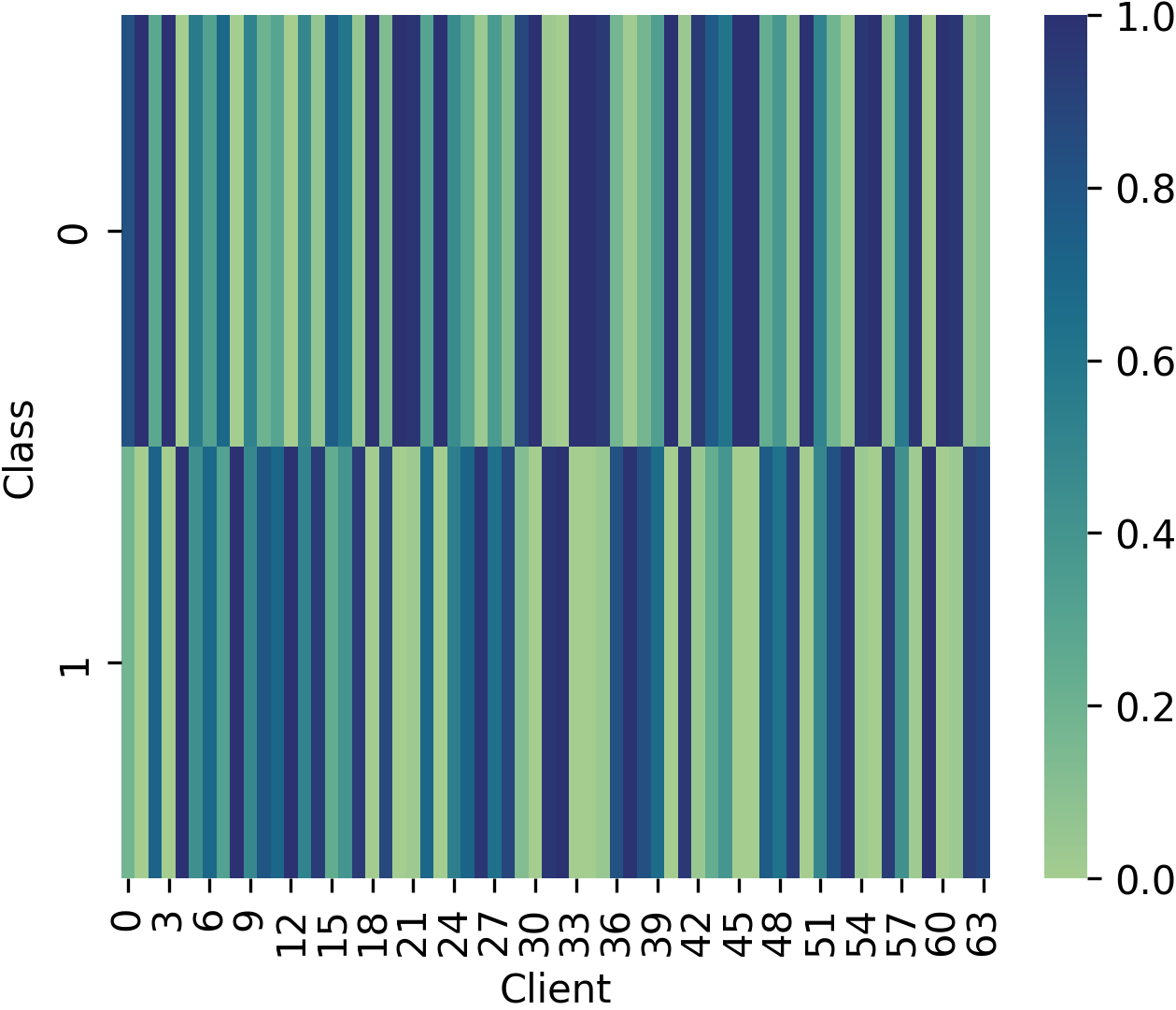
(c) PCam, $\alpha=0.5$

Figure 6: Data Partitioning of each dataset.

Appendix D Visualization

D.1 t-SNE Visualization

We visualize the t-SNE [39] plots of the extracted feature from the server model trained with Full fine-tuning, Head-tuning, FedPEFT-Bias, FedPEFT-Adapter, and FedPEFT-Prompt under the default setting described in Section 4.1, as shown in Figure 7.

We make a few observations here. First, we note that FedPEFT-Bias, FedPEFT-Adapter, and FedPEFT-Prompt are able to reasonably adapt the backbone representation to the target data. With head-tuning, the backbone is kept frozen, and therefore we do not see the same clear separation of each class as with the FedPEFT prototypes. Nonetheless, the frozen backbone does seem to contain relevant semantics, with visible clusters throughout, particularly around the perimeter regions. These observations are consistent with our results and analysis in Section 6.

D.2 Linear Discriminant Analysis of Each Method

We further analyze the Linear Discriminant Analysis (LDA) of the features extracted from the fine-tuned server model for each method, and we interpret the distance to the fully fine-tuned features as the level of fine-tuning. As shown in Figure 8, the features extracted from FedPEFT-Bias are closer to ones extracted from Full fine-tuning compared with FedPEFT-Adapter and FedPEFT-Prompt. We note this as evidence of our statement in Section 6.1 of the main paper: FedPEFT-Bias achieves a higher level of fine-tuning than FedPEFT-Adapter and FedPEFT-Prompt.

Appendix E Broader Impact and Limitation

In the era of the “Foundation Model” [2], large pre-trained models are widely used in many other fields [24, 14]. However, those large models have not been studied in federated learning scenarios due to the large communication burden. Our work aims to address the communication challenge to enable those large models to be considered for federated learning with low communication costs. Furthermore, our work also makes it possible to deploy FL in underdeveloped regions where the communication situation is not ideal. Meanwhile, our work focuses on the training paradigm in FL, which is distinct from other communication reduction methods [22, 38], and can be deployed together in practice.

One limitation of our study is that we only focused on vision transformers as the pre-trained backbone for the experiments. Nonetheless, FedPEFT can be easily adapted to other foundation models, and we regard it as future work.

Figure 7: t-SNE Plots on CIFAR-100. Each dot in the plot means the extracted feature from the fine-tuned server model for one sample, and the color of the dot indicates the ground-truth class of this sample. FedPEFT-Bias, FedPEFT-Adapter, and FedPEFT-Prompt are able to reasonably adapt the backbone representation from ImageNet-21K to the target data. With head-tuning, the backbone is kept frozen, and therefore we do not see the same clear separation of each class as with the FedPEFT prototypes. Nonetheless, the frozen backbone does seem to contain relevant semantics, with visible clusters throughout, particularly around the perimeter regions.

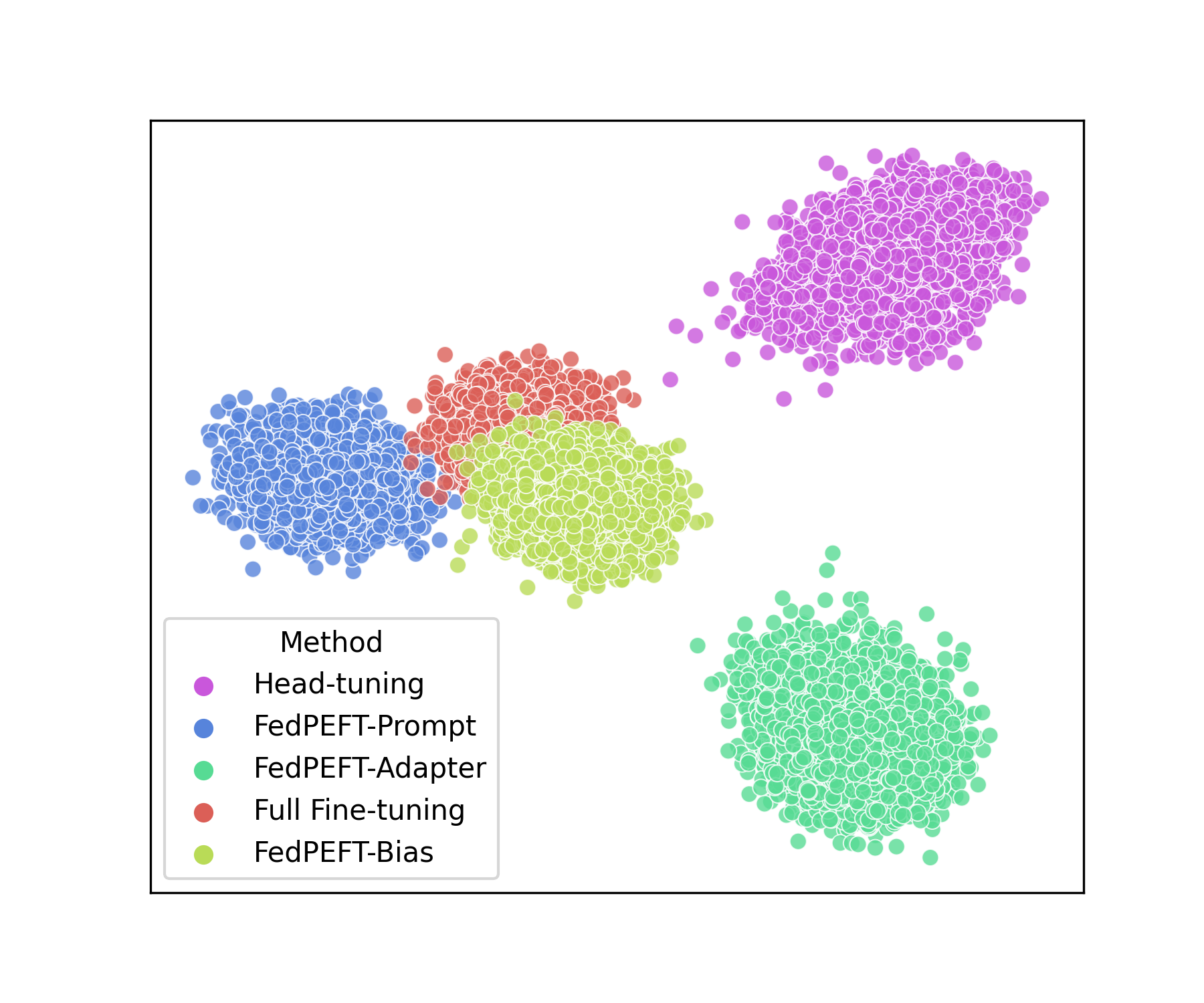
Figure 8: LDA for each method on CIFAR-100. Each cluster shows the extracted features from the server model after fine-tuning for each method. We interpret the distance to the fully fine-tuned features as the degree of fine-tuning. The features extracted from FedPEFT-Bias are closer to ones extracted from Full fine-tuning compared with FedPEFT-Adapter and FedPEFT-Prompt.

Algorithm 2 Pseudocode for FedPEFT-Bias

⬇

class FedPEFT_Bias:

def __init__(basic_model):

self.basic_model = basic_model

# freeze backbone except for the bias terms

for p in self.basic_model.backbone.parameters():

if p is not a bias term:

p.requires_grad = False

def forward(x):

return self.basic_model(x)

Algorithm 3 Pseudocode for FedPEFT-Adapter

⬇

class FedPEFT_Adapter:

def __init__(basic_model, reducation_factor):

self.basic_model = basic_model

num_layers = layer number of basic_model.backbone

# build adapters

self.adapter_downsample = nn.Linear(

embed_dim,

embed_dim // reducation_factor

)

self.adapter_upsample = nn.Linear(

embed_dim // reducation_factor,

embed_dim

)

self.adapter_act_fn = nn.functional.gelu

# freeze backbone

for p in self.basic_model.backbone.parameters():

p.requires_grad = False

def forward(x):

# get the embedding of x

x = embedding(x)

for i in range(num_layers):

# forward normal blocks

block = self.basic_model.blocks[i]

x = x + block.drop_path1(block.ls1(block.attn(block.norm1(x))))

h = x

x = block.drop_path2(block.ls2(block.mlp(block.norm2(x))))

# adapter

adpt = self.adapter_downsample(x)

adpt = self.adapter_act_fn(adpt)

adpt = self.adapter_upsample(adpt)

x = adpt + x

\parx = x + h

\parx = self.basic_model.norm(x)

x = self.basic_model.head(x)

return x

Algorithm 4 Pseudocode for FedPEFT-Prompt

⬇

class FedPEFT_Prompt:

def __init__(basic_model, prompt_num):

self.basic_model = basic_model

num_layers = layer number of basic_model.backbone

# build prompts

prompt_token = = nn.Parameter(

torch.zeros(num_layers, prompt_num, prompt_dim)

)

# freeze backbone

for p in self.basic_model.backbone.parameters():

p.requires_grad = False

def forward(x):

for i in range(len(self.basic_model.blocks)):

torch.cat(prompt_token, x)

x = self.basic_model.blocks[i](x)

x = remove_prompt_tokens

x = self.basic_model.norm(x)

x = self.basic_model.head(x)

References

- [1] Durmus Alp Emre Acar, Yue Zhao, Ramon Matas Navarro, Matthew Mattina, Paul N Whatmough, and Venkatesh Saligrama. Federated learning based on dynamic regularization. arXiv preprint arXiv:2111.04263, 2021.
- [2] Rishi Bommasani et al. On the Opportunities and Risks of Foundation Models, July 2022. arXiv:2108.07258 [cs].
- [3] Han Cai, Chuang Gan, Ligeng Zhu, and Song Han. TinyTL: Reduce Memory, Not Parameters for Efficient On-Device Learning. In Advances in Neural Information Processing Systems, volume 33, pages 11285–11297. Curran Associates, Inc., 2020.
- [4] Mathilde Caron, Hugo Touvron, Ishan Misra, Hervé Jégou, Julien Mairal, Piotr Bojanowski, and Armand Joulin. Emerging Properties in Self-Supervised Vision Transformers. arXiv:2104.14294 [cs], May 2021. arXiv: 2104.14294.
- [5] M. A. P. Chamikara, P. Bertok, I. Khalil, D. Liu, S. Camtepe, and M. Atiquzzaman. Local Differential Privacy for Deep Learning. IEEE Internet of Things Journal, 7(7):5827–5842, July 2020. arXiv:1908.02997 [cs].
- [6] Hao Chen, Ran Tao, Han Zhang, Yidong Wang, Wei Ye, Jindong Wang, Guosheng Hu, and Marios Savvides. Conv-Adapter: Exploring Parameter Efficient Transfer Learning for ConvNets, Aug. 2022. arXiv:2208.07463 [cs].
- [7] Hong-You Chen, Cheng-Hao Tu, Ziwei Li, Han-Wei Shen, and Wei-Lun Chao. On Pre-Training for Federated Learning, June 2022. arXiv:2206.11488 [cs].
- [8] Gong Cheng, Junwei Han, and Xiaoqiang Lu. Remote sensing image scene classification: Benchmark and state of the art. Proceedings of the IEEE, 105(10):1865–1883, 2017.
- [9] Gregory Cohen, Saeed Afshar, Jonathan Tapson, and Andre Van Schaik. Emnist: Extending mnist to handwritten letters. In 2017 international joint conference on neural networks (IJCNN), pages 2921–2926. IEEE, 2017.
- [10] Ivica Dimitrovski, Ivan Kitanovski, Dragi Kocev, and Nikola Simidjievski. Current Trends in Deep Learning for Earth Observation:An Open-source Benchmark Arena for Image Classification. arXiv preprint arXiv:2207.07189, 2022.
- [11] Alexey Dosovitskiy, Lucas Beyer, Alexander Kolesnikov, Dirk Weissenborn, Xiaohua Zhai, Thomas Unterthiner, Mostafa Dehghani, Matthias Minderer, Georg Heigold, Sylvain Gelly, Jakob Uszkoreit, and Neil Houlsby. An Image is Worth 16x16 Words: Transformers for Image Recognition at Scale, June 2021. arXiv:2010.11929 [cs].
- [12] Cynthia Dwork. Differential Privacy: A Survey of Results. In Manindra Agrawal, Dingzhu Du, Zhenhua Duan, and Angsheng Li, editors, Theory and Applications of Models of Computation, Lecture Notes in Computer Science, pages 1–19, Berlin, Heidelberg, 2008. Springer.
- [13] Cynthia Dwork, Aaron Roth, and others. The algorithmic foundations of differential privacy. Foundations and Trends® in Theoretical Computer Science, 9(3–4):211–407, 2014. Publisher: Now Publishers, Inc.
- [14] Andrey Guzhov, Federico Raue, Jörn Hees, and Andreas Dengel. Audioclip: Extending clip to image, text and audio. In ICASSP 2022-2022 IEEE International Conference on Acoustics, Speech and Signal Processing (ICASSP), pages 976–980. IEEE, 2022.
- [15] Jenny Hamer, Mehryar Mohri, and Ananda Theertha Suresh. FedBoost: A Communication-Efficient Algorithm for Federated Learning. In Proceedings of the 37th International Conference on Machine Learning, pages 3973–3983. PMLR, Nov. 2020. ISSN: 2640-3498.
- [16] Ali Hatamizadeh, Hongxu Yin, Holger Roth, Wenqi Li, Jan Kautz, Daguang Xu, and Pavlo Molchanov. GradViT: Gradient Inversion of Vision Transformers, Mar. 2022. arXiv:2203.11894 [cs].
- [17] Kaiming He, Xiangyu Zhang, Shaoqing Ren, and Jian Sun. Deep residual learning for image recognition. In Proceedings of the IEEE conference on computer vision and pattern recognition, pages 770–778, 2016.
- [18] Yangsibo Huang, Samyak Gupta, Zhao Song, Kai Li, and Sanjeev Arora. Evaluating Gradient Inversion Attacks and Defenses in Federated Learning, Nov. 2021. arXiv:2112.00059 [cs] version: 1.
- [19] Menglin Jia, Luming Tang, Bor-Chun Chen, Claire Cardie, Serge Belongie, Bharath Hariharan, and Ser-Nam Lim. Visual Prompt Tuning, July 2022. arXiv:2203.12119 [cs].
- [20] Peter Kairouz et al. Advances and Open Problems in Federated Learning. arXiv:1912.04977 [cs, stat], Mar. 2021. arXiv: 1912.04977.
- [21] Sai Praneeth Karimireddy, Satyen Kale, Mehryar Mohri, Sashank Reddi, Sebastian Stich, and Ananda Theertha Suresh. Scaffold: Stochastic controlled averaging for federated learning. In International Conference on Machine Learning, pages 5132–5143. PMLR, 2020.
- [22] Jakub Konečný, H. Brendan McMahan, Felix X. Yu, Peter Richtárik, Ananda Theertha Suresh, and Dave Bacon. Federated Learning: Strategies for Improving Communication Efficiency, Oct. 2017. arXiv:1610.05492 [cs].
- [23] Alex Krizhevsky. Learning Multiple Layers of Features from Tiny Images. University of Toronto, 2012.
- [24] Liunian Harold Li*, Pengchuan Zhang*, Haotian Zhang*, Jianwei Yang, Chunyuan Li, Yiwu Zhong, Lijuan Wang, Lu Yuan, Lei Zhang, Jenq-Neng Hwang, Kai-Wei Chang, and Jianfeng Gao. Grounded language-image pre-training. In CVPR, 2022.
- [25] Qinbin Li, Bingsheng He, and Dawn Song. Model-Contrastive Federated Learning, Mar. 2021. arXiv:2103.16257 [cs].
- [26] Tian Li, Anit Kumar Sahu, Manzil Zaheer, Maziar Sanjabi, Ameet Talwalkar, and Virginia Smith. Federated Optimization in Heterogeneous Networks, Apr. 2020. arXiv:1812.06127 [cs, stat].
- [27] Haokun Liu, Derek Tam, Mohammed Muqeeth, Jay Mohta, Tenghao Huang, Mohit Bansal, and Colin Raffel. Few-Shot Parameter-Efficient Fine-Tuning is Better and Cheaper than In-Context Learning, Aug. 2022. arXiv:2205.05638 [cs].
- [28] Ningning Ma, Xiangyu Zhang, Hai-Tao Zheng, and Jian Sun. Shufflenet v2: Practical guidelines for efficient cnn architecture design. In Proceedings of the European conference on computer vision (ECCV), pages 116–131, 2018.
- [29] H. Brendan McMahan, Eider Moore, Daniel Ramage, Seth Hampson, and Blaise Agüera y Arcas. Communication-Efficient Learning of Deep Networks from Decentralized Data, Feb. 2017. arXiv:1602.05629 [cs].
- [30] Matias Mendieta, Taojiannan Yang, Pu Wang, Minwoo Lee, Zhengming Ding, and Chen Chen. Local Learning Matters: Rethinking Data Heterogeneity in Federated Learning. arXiv:2111.14213 [cs], Mar. 2022. arXiv: 2111.14213.
- [31] John Nguyen, Kshitiz Malik, Maziar Sanjabi, and Michael Rabbat. Where to Begin? Exploring the Impact of Pre-Training and Initialization in Federated Learning, June 2022. arXiv:2206.15387 [cs].
- [32] Junting Pan, Ziyi Lin, Xiatian Zhu, Jing Shao, and Hongsheng Li. Parameter-Efficient Image-to-Video Transfer Learning, June 2022. arXiv:2206.13559 [cs].
- [33] Jonas Pfeiffer, Andreas Rücklé, Clifton Poth, Aishwarya Kamath, Ivan Vulić, Sebastian Ruder, Kyunghyun Cho, and Iryna Gurevych. AdapterHub: A Framework for Adapting Transformers. In Proceedings of the 2020 Conference on Empirical Methods in Natural Language Processing: System Demonstrations, pages 46–54, Online, 2020. Association for Computational Linguistics.
- [34] Tal Ridnik, Emanuel Ben-Baruch, Asaf Noy, and Lihi Zelnik-Manor. ImageNet-21K Pretraining for the Masses, Aug. 2021. arXiv:2104.10972 [cs].
- [35] Sebastian Ruder. An overview of gradient descent optimization algorithms, June 2017. arXiv:1609.04747 [cs].
- [36] Olga Russakovsky, Jia Deng, Hao Su, Jonathan Krause, Sanjeev Satheesh, Sean Ma, Zhiheng Huang, Andrej Karpathy, Aditya Khosla, Michael Bernstein, Alexander C. Berg, and Li Fei-Fei. ImageNet Large Scale Visual Recognition Challenge. International Journal of Computer Vision (IJCV), 115(3):211–252, 2015.
- [37] Zhiqiang Shen, Zechun Liu, Jie Qin, Marios Savvides, and Kwang-Ting Cheng. Partial Is Better Than All: Revisiting Fine-tuning Strategy for Few-shot Learning, Feb. 2021. arXiv:2102.03983 [cs].
- [38] Ananda Theertha Suresh, Felix X. Yu, Sanjiv Kumar, and H. Brendan McMahan. Distributed Mean Estimation with Limited Communication, Sept. 2017. arXiv:1611.00429 [cs].
- [39] Laurens Van der Maaten and Geoffrey Hinton. Visualizing data using t-sne. Journal of machine learning research, 9(11), 2008.
- [40] Farshid Varno, Marzie Saghayi, Laya Rafiee, Sharut Gupta, Stan Matwin, and Mohammad Havaei. Minimizing Client Drift in Federated Learning via Adaptive Bias Estimation. arXiv:2204.13170 [cs], Apr. 2022. arXiv: 2204.13170.
- [41] Bastiaan S Veeling, Jasper Linmans, Jim Winkens, Taco Cohen, and Max Welling. Rotation Equivariant CNNs for Digital Pathology. June 2018. _eprint: 1806.03962.
- [42] Jianyu Wang, Qinghua Liu, Hao Liang, Gauri Joshi, and H Vincent Poor. Tackling the objective inconsistency problem in heterogeneous federated optimization. Advances in neural information processing systems, 33:7611–7623, 2020.
- [43] Jianyu Wang, Qinghua Liu, Hao Liang, Gauri Joshi, and H. Vincent Poor. Tackling the Objective Inconsistency Problem in Heterogeneous Federated Optimization, July 2020. arXiv:2007.07481 [cs, stat].
- [44] Yaqing Wang, Quanming Yao, James Kwok, and Lionel M. Ni. Generalizing from a Few Examples: A Survey on Few-Shot Learning. Apr. 2019.
- [45] Ross Wightman. PyTorch Image Models, 2019. Publication Title: GitHub repository.
- [46] Mikhail Yurochkin, Mayank Agarwal, Soumya Ghosh, Kristjan Greenewald, Trong Nghia Hoang, and Yasaman Khazaeni. Bayesian Nonparametric Federated Learning of Neural Networks, May 2019. arXiv:1905.12022 [cs, stat].