Tensor-reduced atomic density representations

Abstract

Density based representations of atomic environments that are invariant under Euclidean symmetries have become a widely used tool in the machine learning of interatomic potentials, broader data-driven atomistic modelling and the visualisation and analysis of materials datasets. The standard mechanism used to incorporate chemical element information is to create separate densities for each element and form tensor products between them. This leads to a steep scaling in the size of the representation as the number of elements increases. Graph neural networks, which do not explicitly use density representations, escape this scaling by mapping the chemical element information into a fixed dimensional space in a learnable way. By exploiting symmetry, we recast this approach as tensor factorisation of the standard neighbour density based descriptors and, using a new notation, identify connections to existing compression algorithms. In doing so, we form compact tensor-reduced representation of the local atomic environment whose size does not depend on the number of chemical elements, is systematically convergable and therefore remains applicable to a wide range of data analysis and regression tasks.

Over the past decade, machine learning methods for studying atomistic systems have become widely adopted [1, 2, 3]. Most of these methods utilise representations of local atomic environments that are invariant under relevant symmetries; typically rotations, reflections, translations and permutations of equivalent atoms [4]. Enforcing these symmetries allows for greater data efficiency during model training and ensures that predictions are made in a physically consistent manner. There are many different ways of constructing such representations which are broadly split into two categories: (i) descriptors based on internal coordinates, such as the Behler-Parrinello Atom-Centered Symmetry Functions [5], and (ii) density-based descriptors such as SOAP [6] or the bispectrum [7, 8], which employ a symmetrised expansion of $\nu$-correlations of the atomic neighbourhood density ($\nu=2$ for SOAP and $\nu=3$ for the bispectrum). A major drawback of all these representations is that their size increases dramatically with the number of chemical elements $S$ in the system. For instance, the number of features in the linearly complete ACE [9, 10] descriptor which unifies, extends and generalises the aforementioned representations, scales as $S^{\nu}$ for terms with correlation order $\nu$ (i.e. a body order of $\nu+1)$. This poor scaling severely restricts the use of these representations in many applications. For example, in the case of machine learned interatomic potentials for systems with many (e.g. more than 5) different chemical elements, the large size of the models results in memory limitations being reached during parameter estimation as well as significantly reducing evaluation speed.

Multiple strategies to tackle this scaling problem have been proposed including element weighting [11, 12] or embedding the elements into a fixed small dimensional space [13, 14], directly reducing the element-sensitive correlation order [15], low-rank tensor-train approximations for lattice models [16] and data-driven approaches for selecting the most relevant subset or combination of the original features for a given dataset [17, 18, 19]. A rather different class of machine learning methods are MPNN [20, 21]. Instead of constructing full tensor products, these models also embed chemical element information in a fixed size latent space using a learnable transformation $\mathbb{R}^{S}\rightarrow\mathbb{R}^{K}$ where $K$ is the dimension of the latent space, and thus avoid the poor scaling with the number of chemical elements. Recently these methods have achieved very high accuracy [22, 23, 24], strongly suggesting that the true complexity of the relevant chemical element space does not grow as $S^{\nu}$.

In this paper we introduce a general approach for significantly reducing the scaling of density-based representations like SOAP and ACE. We show that by exploiting the tensor structures of the descriptors and applying low-rank approximations we can derive new tensor-reduced descriptors which are systematically convergeable to the original full descriptor limit. We also verify this with numerical experiments on real data. We also show that there is a natural generalisation to compress not only the chemical element information but also the radial degrees of freedom, yielding an even more compact representation. When fitting interatomic potentials for organic molecules and high entropy alloys, we achieve a ten-fold reduction in the number of features required when using linear (ACE) and nonlinear kernel models (SOAP-GAP). We also fit a linear model to a dataset with 37 chemical elements which would be infeasible without the tensor-reduced features.

All many-body density based descriptors can be understood in terms of the Atomic Cluster Expansion [9]. In ACE, the first step in describing the local neighbourhood $\mathcal{N}(i)=\{j:r_{ij}<r_{\rm cut}\}$ around atom $i$ is forming the one-particle basis $\phi_{znlm}({\bm{r}}_{ij},Z_{j})$ as a product of radial basis functions $R_{n}$, spherical harmonics $Y_{l}^{m}$ and an additional element index shown in Eq. (1), where ${\bm{r}}_{ij}$ and $Z_{j}$ denote the relative position and atomic number of neighbour $j$. Permutation invariance is introduced by summing over neighbour atoms in Eq. (2) after which $(\nu+1)$-body features are formed in Eq. (3) by taking tensor products of the atomic basis $A_{i,znlm}$ with itself $\nu$ times. Finally, Eq. (4) shows how the product basis ${\bm{A}}_{i,{\bm{z}}{\bm{n}}{\bm{l}}{\bm{m}}}$ is rotationally symmetrised using the generalised Clebsch-Gordon coefficients $\mathcal{C}^{{\bm{l}}\eta}_{\bm{m}}$, where $\eta$ enumerates all possible symmetric couplings cf. [9, 10, 17] for the details.

$$\phi_{znlm}({\bm{r}}_{ij},Z_{j}) =R_{n}(r_{ij})Y_{l}^{m}(\hat{{\bm{r}}}_{ij})\delta_{zZ_{j}},$$ (1)

$$A_{i,znlm} =\sum_{j\in\mathcal{N}(i)}\phi_{znlm}({\bm{r}}_{ij},Z_{j}),$$ (2)

$${\bm{A}}_{i,{\bm{z}}{\bm{n}}{\bm{l}}{\bm{m}}} =\prod_{t=1}^{\nu}A_{i,z_{t}n_{t}l_{t}m_{t}}$$ (3)

$${\bm{B}}_{i,{\bm{z}}{\bm{n}}{\bm{l}}\eta} =\sum_{{\bm{m}}}\mathcal{C}^{{\bm{l}}\eta}_{{\bm{m}}}{\bm{A}}_{i,{\bm{z}}{\bm{n}}{\bm{l}}{\bm{m}}}$$ (4)

A linear ACE model can the be fit to an invariant atomic property $\varphi_{i}$ as

$$\varphi_{i}=\sum_{{\bm{z}}{\bm{n}}{\bm{l}}\eta}c_{{\bm{z}}{\bm{n}}{\bm{l}}\eta}{\bm{B}}_{i,{\bm{z}}{\bm{n}}{\bm{l}}\eta}$$ (5)

where $c_{{\bm{z}}{\bm{n}}{\bm{l}}\eta}$ are the model parameters and for practical reasons the expansion is truncated using $\nu_{\mathrm{max}}$, $l_{\mathrm{max}}$ and $n_{\mathrm{max}}=N$. Note that as ${\bm{B}}_{i,{\bm{z}}{\bm{n}}{\bm{l}}\eta}$ is invariant under ${(z_{a},n_{a},l_{a})\xleftrightarrow{}(z_{b},n_{b},l_{b})}$ symmetrically equivalent terms are usually omitted from Eq. (5), again see [9, 10, 17] for the details.

Crucially, the tensor product in Eq. (3) causes the number of features (and therefore the number of model parameters) to grow rapidly as $\mathcal{O}(N^{\nu}S^{\nu})$. Previous work [13, 18] has reduced this to $\mathcal{O}(K^{\nu})$ by first embedding the chemical and radial information into $K$ channels (Eq. (6)), then taking a full tensor product across the $\bar{A}_{i,klm}$ (Eq. (7)).

$$\bar{A}_{i,klm} =\sum_{zn}W^{k}_{zn}A_{i,znlm},\quad k=1\ldots K$$ (6)

$$\bar{{\bm{A}}}_{i,{\bm{k}}{\bm{l}}{\bm{m}}} =\prod_{t=1}^{\nu}\bar{A}_{i,k_{t}l_{t}m_{t}}$$ (7)

This approach is also used in Moment Tensor Potentials [14, 25] and in Gaussian Moment descriptors [26]. The embedding can be identified in Eq. 3 of ref. [25], where $\mu$ indexes the embedded channels and $\nu$ is similar to $l$ in ACE. Then taking tensor products across the embedded channels corresponds to forming products of the moments $M_{\mu\nu}$. In general, the embedding weights are optimised either before or during fitting [13, 25] with the latter causing the models to be non-linear.

We propose a principled approach to further reduce the size of the basis to $\mathcal{O}(K)$ which can be understood from two different angles. First, we identify the model parameters $\bm{c}_{\eta}\equiv c_{{\bm{z}}{\bm{n}}{\bm{l}}\eta}$ in Eq. (5) as a symmetric tensor, invariant under $(z_{a},n_{a},l_{a})\xleftrightarrow{}(z_{b},n_{b},l_{b})$, which can be expanded as a sum of products of rank-1 tensors as,

$$\bm{c}_{\eta}=\sum_{k=1}^{K}\lambda_{k\eta}\underset{\nu\text{ times}}{\underbrace{{\bm{w}}_{k}\otimes{\bm{w}}_{k}\dots\otimes{\bm{w}}_{k}}},$$ (8)

or in component form

$$c_{{\bm{z}}{\bm{n}}{\bm{l}}\eta}=\sum_{k}^{K}\lambda_{k\eta}\prod_{t=1}^{\nu}W^{k}_{z_{t}n_{t}l_{t}}$$ (9)

where $W^{k}_{z_{t}n_{t}l_{t}}$ are the components of ${\bm{w}}_{k}$. This expansion is exact for finite $K$, as $\bm{c}$ is finite due to basis truncation, and is equivalent to eigenvalue decomposition of a symmetric matrix when $\nu=2$. Note that we choose to use the same weights $W^{k}_{z_{t}n_{t}l_{t}}$ for all $\nu$ and $\eta$, which significantly reduces the number of weights that need be specified. In practice, we can choose to expand over the ${\bm{z}}{\bm{n}}$ or ${\bm{z}}$ indices only, see SI for details, and then substitute the expansion into Eq. (5) as

$$\varphi_{i} \approx\sum_{k{\bm{l}}\eta}\lambda_{k{\bm{l}}\eta}\left[\sum_{{\bm{m}}}\mathcal{C}^{{\bm{l}}\eta}_{{\bm{m}}}\sum_{{\bm{z}}{\bm{n}}}\prod_{t=1}^{\nu}W^{kl_{t}}_{z_{t}n_{t}}A_{i,z_{t}n_{t}l_{t}m_{t}}\right]$$ (10)

$$=\sum_{k{\bm{l}}\eta}\lambda_{k{\bm{l}}\eta}\left[\sum_{{\bm{m}}}\mathcal{C}^{{\bm{l}}\eta}_{{\bm{m}}}\prod_{t=1}^{\nu}\tilde{A}_{i,kl_{t}m_{t}}\right]$$ (11)

$$=\sum_{k{\bm{l}}\eta}\lambda_{k{\bm{l}}\eta}{\tilde{\bm{B}}}_{i,k{\bm{l}}\eta}$$ (12)

where ${\tilde{\bm{B}}}_{i,k{\bm{l}}\eta}$ are the new tensor reduced features and the approximation arises because in practice we truncate the tensor decomposition early. The key novelty is that only element-wise products are taken across the $k$ index of the embedded channels $\tilde{A}_{i,kl_{t}m_{t}}$ when forming the many-body basis, rather than a full tensor product, i.e. $k$ does not have a $t$ subscript in Eq. 10 (see Table 1 for the full definitions). For completeness, we note that applying this tensor reduction to the elements only and using $K=2$ is equivalent to the element-weighting strategies used in [11, 12, 27].

There are multiple natural strategies for specifying the embedding weights $W^{kl}_{zn}$, including approximating a pre-computed $c_{{\bm{z}}{\bm{n}}{\bm{l}}\eta}$ or treating the weights as model parameters to be estimated during the training process, as is done in MACE [24]. Here we investigate using random weights as a simpler alternative. This ensures that Eq. 12 remains a linear model and allows the ${\tilde{\bm{B}}}_{i,k{\bm{l}}\eta}$ to be used directly in other tasks such as data visualisation.

Table 1: The density projection $\vec{A}_{i}$ are viewed as vectors with a composite index $(z,n,l,m)$ whereas the embedded density projections $\bar{A}_{i}=(\bm{W}\vec{A}_{i})$ etc. are indexed by $(k,l,m)$. The most general tensor reduced many body density projection (“Tensor sketch”) and its special case (“Tensor decomposition”) are shown together with their scaling with the number of radial basis functions, $N$, number of chemical elements, $S$ and number of embedding channels, $K$. The symbol ${\begin{smallmatrix}\otimes^{lm}\vspace{-0.06cm}\\ \odot_{k\hskip 4.41014pt}\end{smallmatrix}}$ means full tensor product across $l$ and $m$ but element-wise product across $k$ whereas $\otimes$ indicates a full tensor product across all indices.

Name	Product Basis	Index Notation	Basis size
ACE	${\bm{A}}_{i}=\vec{A}_{i}\otimes\vec{A}_{i}\dots\otimes\vec{A}_{i}$	${\bm{A}}_{i,{\bm{z}}{\bm{n}}{\bm{l}}{\bm{m}}}=\prod_{t=1}^{\nu}A_{i,z_{t}n_{t}l_{t}m_{t}}$	$\mathcal{O}(NS)^{\nu}$
[9]
Embedding	$\bar{{\bm{A}}}_{i}=(\bm{W}\vec{A}_{i})\otimes(\bm{W}\vec{A}_{i})\dots\otimes(\bm{W}\vec{A}_{i})$	$\bar{{\bm{A}}}_{i,{\bm{k}}{\bm{l}}{\bm{m}}}=\prod_{t=1}^{\nu}\bar{A}_{i,k_{t}l_{t}m_{t}}$	$\mathcal{O}(K^{\nu})$
[13, 18, 14, 28]		$\bar{A}_{i,k_{t}l_{t}m_{t}}=\sum_{zn}W^{k_{t}}_{zn}A_{i,znl_{t}m_{t}}$
Tensor decomposition	$\tilde{{\bm{A}}}_{i}=(\bm{W}\vec{A}_{i}){\begin{smallmatrix}\otimes^{lm}\vspace{-0.06cm}\\ \odot_{k\hskip 4.41014pt}\end{smallmatrix}}(\bm{W}\vec{A}_{i})\dots\begin{smallmatrix}\otimes^{lm}\vspace{-0.06cm}\\ \odot_{k\hskip 4.41014pt}\end{smallmatrix}(\bm{W}\vec{A}_{i})$	$\tilde{{\bm{A}}}_{i,k{\bm{l}}{\bm{m}}}=\prod_{t=1}^{\nu}\tilde{A}_{i,kl_{t}m_{t}}$	$\mathcal{O}(K)$
[24]		$\tilde{A}_{i,kl_{t}m_{t}}=\sum_{zn}W^{kl_{t}}_{zn}A_{i,znl_{t}m_{t}}$
Tensor sketch	$\hat{{\bm{A}}}_{i}=(\bm{W}^{1}\vec{A}_{i}){\begin{smallmatrix}\otimes^{lm}\vspace{-0.06cm}\\ \odot_{k\hskip 4.41014pt}\end{smallmatrix}}(\bm{W}^{2}\vec{A}_{i})\dots\begin{smallmatrix}\otimes^{lm}\vspace{-0.06cm}\\ \odot_{k\hskip 4.41014pt}\end{smallmatrix}(\bm{W}^{\nu}\vec{A}_{i})$	$\hat{{\bm{A}}}_{i,k{\bm{l}}{\bm{m}}}=\prod_{t=1}^{\nu}\hat{A}_{it,kl_{t}m_{t}}$	$\mathcal{O}(K)$
		$\hat{A}_{it,kl_{t}m_{t}}=\sum_{zn}W^{tk}_{zn}A_{i,znl_{t}m_{t}}$

We now show that the resulting tensor-reduced features can also be understood from the perspective of directly compressing the original ${\bm{B}}_{i,{\bm{z}}{\bm{n}}{\bm{l}}\eta}$ features. RP [29, 30] is an established technique where high dimensional feature vectors $\{{\vec{x}}_{1},\dots,{\vec{x}}_{N}\}\subset\mathbb{R}^{d}$ are compressed as $\tilde{x}_{i}=\bm{W}{\vec{x}}_{i}\in\mathbb{R}^{K}$, with the entries of the matrix $\bm{W}$ being normally distributed. This approach is simple, offers a tuneable level of compression and is underpinned by the Johnson-Lindenstrauss Lemma [31] which bounds the fractional error made in approximating ${\vec{x}}^{T}_{i}{\vec{x}}_{j}$ by $\tilde{x}^{T}_{i}\tilde{x}_{j}$. RP can also be used to reduce the cost of linear models, with a closely related approach recently used in [32]. In CLSR [33, 34, 35] features are replaced by their projections, thus reducing the number of model parameters. Loosely speaking, the approximation errors incurred in CLSR (and RP in general) are expected to decay as $1/\sqrt{K}$ and we refer to refs. [33, 35, 36] for more details. The drawback of RP is that it requires the full feature vector to be constructed so that applying RP to ACE would not avoid the unfavourable $\mathcal{O}(N^{\nu}S^{\nu})$ scaling. We propose using tensor sketching [37] instead of RP. For vectors with tensor structure ${\vec{x}}={\vec{y}}\otimes{\vec{z}}$ where ${\vec{x}}\in\mathbb{R}^{d_{1}d_{2}}$, ${\vec{y}}\in\mathbb{R}^{d_{1}}$ and ${\vec{z}}\in\mathbb{R}^{d_{2}}$, the Random Projection $\bm{W}{\vec{x}}$ can be efficiently computed directly from ${\vec{y}}$ and ${\vec{z}}$ as

$$\bm{W}{\vec{x}}=(\bm{W^{\prime}}{\vec{y}}\,)\odot(\bm{W^{\prime\prime}}{\vec{z}}\,).$$ (13)

where $\odot$ denotes the element-wise (Hadamard) product. Similarly, the ACE product basis can be tensor sketched, across the $zn$ indices, as

$$\hat{{\bm{A}}}_{i}=(\bm{W}^{1}\vec{A}_{i}){\begin{smallmatrix}\otimes^{lm}\vspace{-0.06cm}\\ \odot_{k\hskip 4.41014pt}\end{smallmatrix}}(\bm{W}^{2}\vec{A}_{i})\dots\begin{smallmatrix}\otimes^{lm}\vspace{-0.06cm}\\ \odot_{k\hskip 4.41014pt}\end{smallmatrix}(\bm{W}^{\nu}\vec{A}_{i})$$ (14)

where ${\begin{smallmatrix}\otimes^{lm}\vspace{-0.06cm}\\ \odot_{k\hskip 4.41014pt}\end{smallmatrix}}$ denotes taking the tensor product over the upper indices $lm$ and the element-wise product over the lower index $k$ and $\bm{W}^{1},\bm{W}^{2}$ etc. are i.i.d. random matrices, see SI for details. The $\hat{{\bm{A}}}_{i,k{\bm{l}}{\bm{m}}}$ can then be symmetrised as in Eq. 4 yielding

$$\hat{{\bm{B}}}_{i,k{\bm{l}}\eta}=\sum_{m}\mathcal{C}^{{\bm{l}}\eta}_{\bm{m}}\prod_{t=1}^{\nu}\hat{A}_{it,kl_{t}m_{t}}$$ (15)

where $\hat{A}_{it,kl_{t}m_{t}}$ is defined more precisely in Table 1. Finally, we note that because the embedded channels are independent, the error in approximating inner products using the average across $K$ channels is expected to decrease as $1/\sqrt{K}$, just as with standard RP. Based on this, we conjecture that similar bounds derived for the errors made in CLSR may also apply here. A summary comparing standard ACE, element-embedding and tensor-reduced ACE is given in Table 1, where it is clear that The features derived using tensor decomposition are equivalent to the tensor-sketched features with the choice of using equal weights in each factor.

We now turn to numerical results and first demonstrate that the tensor-reduced features are able to efficiently and completely describe a many-element training set. We consider a dataset comprised of all symmetry inequivalent fcc structures made up of 5 elements with up to 6 atoms per unit cell [38]. A set of features is complete on this dataset if the design matrix for a linear model fit to total energies has full (numerical) row rank, where each row corresponds to a different training configuration.

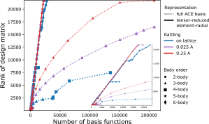
Figure 1: The row rank of the design matrix as a function of basis set on a dataset of all symmetry inequivalent fcc lattices of 5 chemical elements and unit cell sizes of up to 6 atoms. The inset zooms in on the $x=y$ region.

Figure 1 shows the numerical rank of the design matrix as a function of the basis set. At a given correlation order the standard ACE basis set is grown by increasing the polynomial degree, and the tensor-reduced basis set is enlarged by increasing $K$, the number of independent channels. In both cases once the rank stops increasing at the given correlation order we increment $\nu$. The colors in Fig. 1 correspond to three different geometrical variations: blue contains on-lattice configurations only whilst in magenta and red the atomic positions have been perturbed by a random Gaussian displacement with mean 0 and standard deviation of 0.025 and 0.25 Å, respectively. The dotted lines corresponds to the standard ACE basis, whereas the solid lines corresponds to the tensor-reduced version from Eq. (12). Although the standard ACE basis can always achieve full row rank since it is a complete linear basis, it does this very inefficiently. In contrast, the row rank using the tensor-reduced basis grows almost linearly. Thus the tensor-reduced basis, having removed unnecessary redundancies, still retains the expressive power of the full basis.

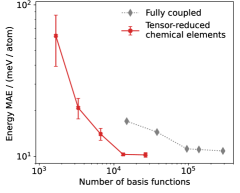
Figure 2: Convergence of the energy errors of organic molecules on the independent test set with respect to the number of basis functions is shown for linear models using standard and tensor-reduced (tensor decomposition) ACE features. Error bars show the standard error in the mean, computed across 5 fits using independently chosen random weights.

Next, we fit a linear ACE [39] model on a training set of 400 different organic molecules of size 19-168 atoms, randomly selected from the QMugs dataset [40] that are made up of 10 different chemical elements (H, C, N, O, F, P, S, Cl, Br, I). The conformers were created by running GFN2-xTB [41] 800 K NVT molecular dynamics for 1 ps starting from a published minimum energy structure. The test set is composed of 1,000 different molecules sampled the same way. This is a small-data regime task that is particularly challenging due to the chemical and conformational diversity. Figure 2 shows the convergence of the energy error with the number of basis functions for the fully coupled and the tensor-reduced ACE models, both using $\nu_{\mathrm{max}}=3$ (4-body). By increasing the number of uncoupled channels $K$ we can converge the accuracy to the previous level, whilst reducing the size of the model by a factor of 10.

The tensor reduction techniques proposed in this work can be directly applied to other density based descriptors and used with alternative models. To demonstrate this we used the tensor-reduced SOAP power spectrum to fit GAP [7] models to the quinary high-entropy alloy dataset from ref. [42]. The descriptors were computed using turbo-soap [43] and fitting was performed using the GAP code [44]. To provide a baseline for comparison, reference models were fit using the full power spectrum evaluated with a varying number of basis functions; $n_{\text{max}}=2l_{\text{max}}$. All compressed descriptors were constructed using the largest values of $n_{\mathrm{max}}=8,l_{\mathrm{max}}=4$, see Supplemental Material [45] for details. The force errors achieved on the independent test set are shown as a function of descriptor length in Fig. 3. For this dataset, mixing only the chemical elements did not help, which is likely due to the minimal savings made as a result of the low correlation order. However, using the fully element-radial tensor-reduced descriptor allowed for similar accuracy to be achieved using approximately 10 times fewer features. Furthermore, the errors achieved with all compressed descriptors are shown to converge to the error achieved with the full SOAP vector they were derived from. Finally, in the high accuracy regime, descriptor length > 300, models using the tensor-sketch element-radial reduction matched the accuracy achieved using full RP.

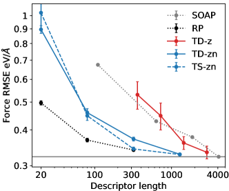
Figure 3: Convergence of force RMSE on the high-entropy alloy test set as a function of descriptor length for various GAP models. Error bars show the standard error in the mean, computed across 5 fits using independently chosen random weights. The tensor reduction is denoted using TD for tensor-decomposition (12), TS for tensor-sketching (15) and the reduction is performed over the indices after the hyphen.

The information content of these SOAP based descriptors was also measured using the information imbalance [46]. It was found that the fully element-radial tensor reduced descriptors offered comparable data efficiency to a random projection and that taking an element-wise product across embedded channels outperformed taking a full tensor product, see Supplemental Material [45] for details.

Finally, we assess the effect of optimising the embedding weights using the MACE architecture [24]. A typical MACE model is a 2-layer message passing network which utilises tensor-reduced ACE features to efficiently represent equivariant body-ordered messages. Normally, the embedding weights are optimised using backpropagation along with all other model parameters, but it is possible to fix these weights to random values. As such, whilst a multi-layer MACE is a complex non-linear network model, a single-layer MACE with frozen embedding weights is equivalent to a linear model using tensor-reduced ACE features [23]. Furthermore, within MACE the embedding weights used in the tensor decomposition, see Table 1, are approximated as $W^{kl_{t}}_{zn}$ = $U_{zn}V^{kl_{t}}_{n}$ so that the element weights $U_{zn}$ and the radial weights $V^{kl_{t}}_{n}$ can be optimised or frozen independently.

We use the HME21 dataset [47, 48] for this test due to its exceptional diversity, both chemically with 37 elements, and structurally with configurations including isolated molecules, bulk crystals, surfaces, clusters and disordered materials. We fit several models (see Supplemental Material [45] for details), and the energy and force errors on the independent test set are summarised in Table 2. Strikingly, using random element embedding weights leads to almost no degradation in model accuracy compared to using optimised element embedding weights. In contrast, randomizing both the element and radial embedding weights lead to significantly larger prediction errors. A two-layer model with optimised weights achieves state of the art accuracy on HME21, showing the power of the message passing architecture and further highlighting the effectiveness of the tensor-reduced features.

Table 2: Mean absolute errors on the HME21 dataset. Energy ($E$, meV) and force ($F$, eV/Å) errors of models. The labels, (1) or (2), of the MACE models indicate the number of message passing layers.

		MACE $(1)$	MACE $(1)$	MACE $(1)$	MACE $(2)$	TeaNet [49]	NequIP [22]
	$U_{zn}$	opt	rand	rand	opt
	$V^{kl_{t}}_{n}$	opt	opt	rand	opt
	$E$	53.5	52.1	254.8	15.7	19.6	47.8
	$F$	0.189	0.175	0.456	0.138	0.174	0.199

In conclusion, we introduced a tensor-reduced form of the ACE basis for modelling symmetric functions of local atomic neighbour environments that eliminates the $\mathcal{O}\left(N^{\nu}S^{\nu}\right)$ scaling of the basis set size with the number of chemical elements and radial basis functions. Intuitively, the construction can be thought of as mixing the element and radial channels and then only coupling these channels to themselves when constructing the higher order many-body basis. We derived this new embedded basis from a symmetric tensor decomposition and explored its connection to tensor-sketching. We showed that this reduced basis is also systematic, and that in practice it can enable a 10-fold reduction in basis set size for diverse datasets with many elements, including organic molecules and high entropy alloys. When using in a 2-layer message passing network, MACE[24], the tensor-decomposition yields state of the art performance.

Supplemental Material

.1 Symmetric Tensor Decomposition of $c_{{\bm{z}}{\bm{n}}{\bm{l}}\eta}$

We start by relabelling the parameter tensor $c_{{\bm{z}}{\bm{n}}{\bm{l}}\eta}$ of Eq. (5) to $c_{{\bm{n}}{\bm{l}}\eta}$ where the element index has been incorporated into ${\bm{n}}=((z_{1},n_{1}),(z_{2},n_{2}),...(z_{\nu},n_{\nu}))$. Then we remove the lexicographical ordering of $({\bm{z}},{\bm{n}},{\bm{l}})$ and retain all terms in the tensor-product so that there are redundancies in ${\bm{B}}_{i,{\bm{n}}{\bm{l}}\eta}$. The advantage of this is that the generalised Clebsch-Gordon coefficients do not depend on ${\bm{n}}$, which simplifies this analysis. Next we note that $c_{{\bm{n}}{\bm{l}}\eta}$ is symmetric under $(n_{i},l_{i})\xleftrightarrow{}(n_{j},l_{j})$, but not $n_{i}\xleftrightarrow{}n_{j}$ or $l_{i}\xleftrightarrow{}l_{j}$. We can now use the fact that a symmetric tensor can be expanded in terms of rank-1 tensors, i.e.

$$\bm{c}=\sum_{k}\lambda_{k}{\bm{w}}^{k}\otimes{\bm{w}}^{k}\otimes\dots\otimes{\bm{w}}^{k}$$ (16)

or, rewritten in component form,

$$c_{{\bm{n}}{\bm{l}}\eta}\sim\sum_{k}^{K}\lambda_{k\eta}[{\bm{w}}^{k}]^{l_{1}}_{n_{1}}\cdots[{\bm{w}}^{k}]^{l_{\nu}}_{n_{\nu}}$$ (17)

where the components of ${\bm{w}}^{k}$ are indexed with the tuple $(n_{i},l_{i})$ as $[{\bm{w}}^{k}]^{l_{i}}_{n_{i}}=w^{kl_{i}}_{n_{i}}$. Note that the same set of ${\bm{w}}^{k}$ are used to expand all $c_{{\bm{n}}{\bm{l}}\eta}$, rather than having a separate set for each $({\bm{l}},\eta)$ tuple. Consequently the expansion for each $({\bm{l}},\eta)$ will converge slower, although we stress that it is still systematic, but crucially we require far fewer embedded one particle basis functions. We then insert this expression into

$$\varphi=\sum_{{\bm{l}}{\bm{m}}\eta}{\bm{C}}^{\eta}_{{\bm{l}}{\bm{m}}}\sum_{{\bm{n}}}c_{{\bm{n}}{\bm{l}}\eta}{\bm{A}}_{{\bm{n}}{\bm{l}}{\bm{m}}}.$$ (18)

and get

$$\sum_{{\bm{n}}}c_{{\bm{n}}{\bm{l}}\eta}{\bm{A}}_{{\bm{n}}{\bm{l}}{\bm{m}}} =\sum_{{\bm{n}}}\sum_{k}\lambda_{k\eta}\prod_{t=1}^{\nu}w^{kl_{t}}_{n_{t}}A_{n_{t}l_{t}m_{t}}$$ (19)

$$=\sum_{k}\lambda_{k\eta}\sum_{{\bm{n}}}\prod_{t=1}^{\nu}w^{kl_{t}}_{n_{t}}A_{n_{t}l_{t}m_{t}}$$ (20)

$$=\sum_{k}\lambda_{k\eta}\prod_{t=1}^{\nu}\sum_{n}w^{kl_{t}}_{n}A_{nl_{t}m_{t}}$$ (21)

$$=\sum_{k}\lambda_{k\eta}\prod_{t=1}^{\nu}\tilde{A}_{k,l_{t},m_{t}}$$ (22)

where

$$\tilde{A}_{k,l_{t},m_{t}} =\sum_{n}w^{kl_{t}}_{n}A_{nl_{t}k_{t}}$$ (23)

$$=\sum_{n}w^{kl_{t}}_{n}\sum_{j}R_{nl_{t}}(r_{j})Y_{l_{t}}^{m_{t}}(\hat{\bm{r}}_{j})$$ (24)

$$=\sum_{j}\bigg{[}\sum_{n}w^{kl_{t}}_{n}R_{nl_{t}}(r_{j})\bigg{]}Y_{l_{t}}^{m_{t}}(\hat{\bm{r}}_{j})$$ (25)

$$=:\sum_{j}\tilde{R}_{kl_{t}}(r_{j})Y_{l_{t}}^{m_{t}}(\hat{\bm{r}}_{j}).$$ (26)

and $\tilde{R}_{kl_{t}}(r_{j})=\sum_{n}w^{kl_{t}}_{n}R_{nl_{t}}(r_{j})$ is a mixed element-radial basis function. Subbing Eq. (26) back into Eq. (18) we arrive at

$$\varphi =\sum_{k\eta}\lambda_{k\eta}{\tilde{\bm{B}}}_{k\eta}$$ (27)

$${\tilde{\bm{B}}}_{k\eta} =\sum_{{\bm{l}}{\bm{m}}}{\bm{C}}^{\eta}_{{\bm{l}}{\bm{m}}}\tilde{{\bm{A}}}_{k{\bm{l}}{\bm{m}}},$$ (28)

$$\tilde{{\bm{A}}}_{k{\bm{l}}{\bm{m}}} =\prod_{t}\tilde{A}_{kl_{t}m_{t}}.$$ (29)

Where each basis function ${\tilde{\bm{B}}}_{k\eta}$ involves a sum over all ${\bm{l}}$ tuples at the given correlation order. An alternative option is to decompose $c_{{\bm{n}}{\bm{l}}\eta}$ approximately as

$$c_{{\bm{n}}{\bm{l}}\eta}\sim\sum_{k}^{k_{\mathrm{max}}}\lambda_{k{\bm{l}}\eta}[{\bm{w}}^{kl_{1}}]_{n_{1}}\cdots[{\bm{w}}^{kl_{\nu}}]_{n_{\nu}},$$ (30)

where the difference is that $[{\bm{w}}^{k}]^{l_{i}}_{n_{i}}\rightarrow[{\bm{w}}^{kl_{i}}]_{n_{i}}$. Proceeding as above results in the identical analysis as before, except that now the basis functions become

$$\varphi =\sum_{k{\bm{l}}}\lambda_{k{\bm{l}}\eta}{\tilde{\bm{B}}}_{k{\bm{l}}\eta}$$ (31)

$${\tilde{\bm{B}}}_{k{\bm{l}}\eta} =\sum_{{\bm{m}}}{\bm{C}}^{\eta}_{{\bm{l}}{\bm{m}}}\tilde{{\bm{A}}}_{k{\bm{l}}{\bm{m}}}$$ (32)

and $\tilde{{\bm{A}}}_{k{\bm{l}}{\bm{m}}}$ is as above. Both are valid expansions and comparing Eq. (28) and Eq. (32) we see that ${\tilde{\bm{B}}}_{k\eta}=\sum_{\bm{l}}{\tilde{\bm{B}}}_{k{\bm{l}}\eta}$. In this work we choose to investigate using ${\tilde{\bm{B}}}_{k{\bm{l}}\eta}$ as every computed ${\tilde{\bm{B}}}_{k{\bm{l}}\eta}$ is used separately, so that the model is more flexible for a similar evaluation cost. We note that using ${\tilde{\bm{B}}}_{k\eta}$ might result in a greater level of model accuracy for a given basis set size but leave this investigation to future work.

.2 Uncoupled Basis as a Tensor Sketch

Here we investigate whether inner products are preserved when moving from the full ACE basis to the uncoupled basis. Precisely, we investiage whether $\sum_{{\bm{l}}\eta}{\tilde{\bm{B}}}_{i,k{\bm{l}}\eta}{\tilde{\bm{B}}}_{j,k{\bm{l}}\eta}$ from Eq. (12) and $\sum_{{\bm{l}}\eta}{\hat{\bm{B}}}_{i,k{\bm{l}}\eta}{\hat{\bm{B}}}_{j,k{\bm{l}}\eta}$ from Eq. (15) are unbiased estimators for $\sum_{{\bm{z}}{\bm{n}}{\bm{l}}\eta}{\bm{B}}_{i,{\bm{z}}{\bm{n}}{\bm{l}}\eta}{\bm{B}}_{j,{\bm{z}}{\bm{n}}{\bm{l}}\eta}$ from Eq. (5) when the weights $W^{kl}_{zn}$ are drawn from a symmetric distribution with mean 0. We start by combining the element and radial indices so that ${\bm{B}}_{{\bm{z}}{\bm{n}}{\bm{l}}\eta}\rightarrow{\bm{B}}_{{\bm{n}}{\bm{l}}\eta}$. First we note that

$$\sum_{{\bm{n}}{\bm{l}}\eta}{\bm{B}}_{i,{\bm{n}}{\bm{l}}\eta}{\bm{B}}_{j,{\bm{n}}{\bm{l}}\eta} =\sum_{{\bm{n}}{\bm{l}}\eta}\left(\sum_{\bm{m}}{\bm{C}}^{\eta}_{{\bm{l}}{\bm{m}}}{\bm{A}}_{i,{\bm{n}}{\bm{l}}{\bm{m}}}\right)\left(\sum_{{\bm{m}}^{\prime}}{\bm{C}}^{\eta}_{{\bm{l}}{\bm{m}}^{\prime}}{\bm{A}}_{j,{\bm{n}}{\bm{l}}{\bm{m}}^{\prime}}\right)$$ (33)

$$=\sum_{{\bm{l}}{\bm{m}}{\bm{m}}^{\prime}\eta}{\bm{C}}^{\eta}_{{\bm{l}}{\bm{m}}}{\bm{C}}^{\eta}_{{\bm{l}}{\bm{m}}^{\prime}}\left(\sum_{\bm{n}}{\bm{A}}_{i,{\bm{n}}{\bm{l}}{\bm{m}}}{\bm{A}}_{j,{\bm{n}}{\bm{l}}{\bm{m}}^{\prime}}\right)$$ (34)

and similarly

$$\sum_{{\bm{k}}{\bm{l}}\eta}{\hat{\bm{B}}}_{i,{\bm{k}}{\bm{l}}\eta}{\hat{\bm{B}}}_{j,{\bm{k}}{\bm{l}}\eta} =\sum_{{\bm{k}}{\bm{l}}\eta}\left(\sum_{\bm{m}}{\bm{C}}^{\eta}_{{\bm{l}}{\bm{m}}}{\hat{\bm{A}}}_{i,{\bm{k}}{\bm{l}}{\bm{m}}}\right)\left(\sum_{{\bm{m}}^{\prime}}{\bm{C}}^{\eta}_{{\bm{l}}{\bm{m}}^{\prime}}{\hat{\bm{A}}}_{j,{\bm{k}}{\bm{l}}{\bm{m}}^{\prime}}\right)$$ (35)

$$=\sum_{{\bm{l}}{\bm{m}}{\bm{m}}^{\prime}\eta}{\bm{C}}^{\eta}_{{\bm{l}}{\bm{m}}}{\bm{C}}^{\eta}_{{\bm{l}}{\bm{m}}^{\prime}}\left(\sum_{\bm{k}}{\hat{\bm{A}}}_{i,{\bm{k}}{\bm{l}}{\bm{m}}}{\hat{\bm{A}}}_{j,{\bm{k}}{\bm{l}}{\bm{m}}^{\prime}}\right)$$ (36)

where the sum over ${\bm{k}}$ is over randomly chosen tuples $(k_{1},k_{2},...k_{\nu})$ where $k_{i}\neq k_{j}$. Comparing Eq. (34) and Eq. (36) we see that it is sufficient to check that

$$\sum_{\bm{k}}\mathbb{E}[{\hat{\bm{A}}}_{i,{\bm{k}}{\bm{l}}{\bm{m}}}{\hat{\bm{A}}}_{j,{\bm{k}}{\bm{l}}{\bm{m}}^{\prime}}]=\sum_{\bm{n}}{\bm{A}}_{i,{\bm{n}}{\bm{l}}{\bm{m}}}{\bm{A}}_{j,{\bm{n}}{\bm{l}}{\bm{m}}^{\prime}}$$ (37)

Next we note that every ${\bm{k}}$ tuple is independent, so we need only check one term in the sum on the left. Inserting the definition of ${\hat{\bm{A}}}_{{\bm{k}}{\bm{l}}{\bm{m}}}$ we find that

$${\hat{\bm{A}}}_{i,{\bm{k}}{\bm{l}}{\bm{m}}}{\hat{\bm{A}}}_{j,{\bm{k}}{\bm{l}}{\bm{m}}^{\prime}} =\prod_{t}^{\nu}\tilde{A}^{k_{t}}_{i,l_{t}m_{t}}\tilde{A}^{k_{t}}_{j,l_{t}m^{\prime}_{t}}$$ (38)

$$=\prod_{t}^{\nu}\left(\sum_{n}W^{k_{t}l_{t}}_{n}A_{i,nl_{t}m_{t}}\right)\left(\sum_{n^{\prime}}W^{k_{t}l_{t}}_{n^{\prime}}A_{j,n^{\prime}l_{t}m^{\prime}_{t}}\right)$$ (39)

$$=\sum_{{\bm{n}}{\bm{n}}^{\prime}}\prod_{t}^{\nu}W^{k_{t}l_{t}}_{n^{\prime}_{t}}W^{k_{t}l_{t}}_{n_{t}}A_{i,n_{t}l_{t}m_{t}}A_{j,n^{\prime}_{t}l_{t}m^{\prime}_{t}}$$ (40)

$$=\sum_{{\bm{n}}{\bm{n}}^{\prime}}\prod_{t}^{\nu}A_{i,n_{t}l_{t}m_{t}}A_{j,n^{\prime}_{t}l_{t}m^{\prime}_{t}}\prod_{t}^{\nu}W^{k_{t}l_{t}}_{n_{t}}W^{k_{t}l_{t}}_{n^{\prime}_{t}}$$ (41)

Next we take the expectation value

$$\mathbb{E}\left[{\hat{\bm{A}}}_{i,{\bm{k}}{\bm{l}}{\bm{m}}}{\hat{\bm{A}}}_{j,{\bm{k}}{\bm{l}}{\bm{m}}^{\prime}}\right] =\sum_{{\bm{n}}{\bm{n}}^{\prime}}\prod_{t}^{\nu}A_{i,n_{t}l_{t}m_{t}}A_{j,n^{\prime}_{t}l_{t}m^{\prime}_{t}}\mathbb{E}\left[\prod_{t}^{\nu}W^{k_{t}l_{t}}_{n_{t}}W^{k_{t}l_{t}}_{n^{\prime}_{t}}\right]$$ (43)

$$=\sum_{{\bm{n}}{\bm{n}}^{\prime}}\prod_{t}^{\nu}A_{i,n_{t}l_{t}m_{t}}A_{j,n^{\prime}_{t}l_{t}m^{\prime}_{t}}\mathbb{E}\left[W^{2}\right]^{\nu}\delta_{{\bm{n}}{\bm{n}}^{\prime}}$$ (44)

$$=\mathbb{E}\left[W^{2}\right]^{\nu}\sum_{\bm{n}}\prod_{t}^{\nu}A_{i,n_{t}l_{t}m_{t}}A_{j,n_{t}l_{t}m^{\prime}_{t}}$$ (45)

$$=\mathbb{E}\left[W^{2}\right]^{\nu}\sum_{\bm{n}}{\bm{A}}_{i,{\bm{n}}{\bm{l}}{\bm{m}}}{\bm{A}}_{j,{\bm{n}}{\bm{l}}{\bm{m}}}$$ (46)

where $\mathbb{E}\left[W^{k_{i}l_{i}}_{n_{i}}W^{k_{j}l_{j}}_{n^{\prime}_{i}}\right]=\delta_{k_{i}k_{j}}\delta_{l_{i}l_{j}}\delta_{n_{i}n^{\prime}_{i}}\mathbb{E}\left[W^{2}\right]$ because the $W^{k_{i}l_{i}}_{n_{i}}$ are i.i.d. random variables with mean 0. Eq. (46) is the result we require, up to a constant factor of $\mathbb{E}\left[W^{2}\right]^{\nu}$ which can be absorbed into the definition of ${\tilde{\bm{B}}}_{{\bm{k}}{\bm{l}}\eta}$.

The analysis for ${\tilde{\bm{B}}}_{k{\bm{l}}\eta}$ follows in the same way except that we have $\mathbb{E}\left[\prod_{i}^{\nu}W^{k_{i}l_{i}}_{n_{i}}W^{k_{i}l_{i}}_{n^{\prime}_{i}}\right]\rightarrow\mathbb{E}\left[\prod_{i}^{\nu}W^{kl_{i}}_{n_{i}}W^{kl_{i}}_{n^{\prime}_{i}}\right]$ in Eq. (44). If all $l_{i}$ in ${\bm{l}}$ are unique then $\mathbb{E}\left[\prod_{i}^{\nu}W^{kl_{i}}_{n_{i}}W^{kl_{i}}_{n^{\prime}_{i}}\right]=\prod_{i}^{\nu}\mathbb{E}\left[W^{2}\right]\delta_{n_{i}n^{\prime}_{i}}$. However if any of the $l_{i}$ are repeated then there are additional terms which adjust the expectation value e.g. ${\bm{l}}=(2,3,2)$,

$$\mathbb{E}\left[W^{k,2}_{n_{1}}W^{k,2}_{n^{\prime}_{1}}\cdot W^{k,3}_{n_{2}}W^{k,3}_{n^{\prime}_{2}}\cdot W^{k,2}_{n_{3}}W^{k,2}_{n^{\prime}_{3}}\right]=$$ (47)

$$\mathbb{E}[W^{2}]^{3}\left(\delta_{n_{1}n_{1}^{\prime}}\delta_{n_{2}n_{2}^{\prime}}\delta_{n_{3}n_{3}^{\prime}}+\delta_{n_{1}n_{3}}\delta_{n_{2}n^{\prime}_{2}}\delta_{n^{\prime}_{1}n^{\prime}_{3}}+\delta_{n_{1}n^{\prime}_{3}}\delta_{n_{2}n^{\prime}_{2}}\delta_{n^{\prime}_{1}n_{3}}\right)$$ (48)

$$+\left(\mathbb{E}[W^{2}]\mathbb{E}[W^{4}]-3\mathbb{E}[W^{2}]^{3}\right)\delta_{n_{2}n^{\prime}_{2}}\delta_{n_{1},n^{\prime}_{1}}\delta_{n_{1},n_{3}}\delta_{n_{1},n^{\prime}_{3}}$$ (49)

This means that ${\tilde{\bm{B}}}_{k{\bm{l}}\eta}$ from Eq. (12) is not a true tensor sketch.

.3 Details of constructing the ACE basis

.3.1 Rank test

Numerical Rank

The design matrix considered was constructed by evaluating all basis functions on all sites in the unit cell and summing up their values. This way we obtained a matrix $\Psi$ of the size $(\#\text{basis}\times\#\text{configurations})$. The rank of $\Psi$ was computed by counting the number of non-zero singular values of the matrix with a tolerance of $n*\epsilon$, where $n$ is the smallest dimension of the matrix and $\epsilon$ is the machine epsilon of the type Float64 in the Julia programming language $(2.220446049250313e-16)$.

Details of the standard ACE basis

For the ACE basis we used a cutoff radius of 10. The maximum degree of each body-order was increased gradually until the numerical rank stopped increasing. The other parameters of the basis are identical to the one used in [39] as implemented in ACE.jl

Details of the Tensor-reduced ACE basis

For the Tensor-reduced ACE basis we also used a cutoff of 10 Å. At each of the body order we used a maximum radial polynomial degree of 21, meaning that the radial functions were a random combination of the 21 radial polynomials. For the angular part we used maximum L of the spherical harmonics for each of the correlation orders as follows: $1=>0,\quad 2=>12,\quad 3=>10,\quad 4=>8,\quad 5=>6$. The motivation for having lower L for higher correlation order stems from the expectation that higher body order contribution will be smoother.

.3.2 Linear ACE models

The models had a cutoff of 4.5 Å. The models were fitted using linear least squares regression with Laplacian preconditioning regularization as detailed in Ref [39]. The basis size was increased by gradually increasing the maximum polynomial degree of the ACE basis, with the inclusion of up to 4-body basis functions. The Tensor-reduced ACE basis also included up to 4-body features and was grown by increasing the number of embedding channels.

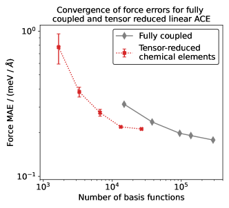
Figure 4: Convergence of linear Tensor-reduced ACE force error to the fully coupled with increasing number of channels. Error bars show the standard error in the mean, computed across 5 fits using independently chosen random weights

We have also trained models by applying the tensor reduction to both the chemical element and the radial channels. In this case we find that the errors do not converge as rapidly resulting in higher errors with similar basis set size compared to the fully coupled basis set. For models with ca. 20,000 basis functions applying tensor reduction to chemical elements only gives 0.2 eV/Å, chemical element - radial tensor reduction gives 0.5 eV/Å, whereas the fully coupled basis set has an error of 0.3 eV/Å. This observation is common to the linear ACE and one-layer MACE (which is an alternative implementation of linear ACE), but is different from the behaviour of the kernel regression based radial-element reduced SOAP kernel model. We hypothesise that whilst the chemical element degrees of freedom can efficiently be decoupled the radial decoupling only works in the case of non-linear models.

.4 SOAP Information Imbalance

Next, we investigate tensor-reduced forms of the SOAP power spectrum. The information imbalance, introduced in ref. [46], provides a quantitative way to measure the relative information content of descriptors by comparing the pairwise distances between atomic environments in a given dataset. For a given environment, all other environments in the dataset are ranked (denoted by $r$) according to their distance from it using two different descriptors $A$ and $B$. The information imbalance is then defined as

$$\Delta_{B\rightarrow A}=\frac{2}{n_{\mathrm{env}}}\langle r_{B}|r_{A}=1\rangle$$ (50)

where $r_{B}|r_{A}=1$ is the rank according to $B$ of the nearest neighbour according to $A$ and the average $\langle r_{B}|r_{A}=1\rangle$ is across all $n_{\mathrm{env}}$ environments in the dataset. Defined as such, for large $n_{\mathrm{env}}$, $\Delta_{B\rightarrow A}\approx 0$ when $B$ contains the same information as $A$ and $\Delta_{B\rightarrow A}\approx 1$ if $B$ contains no information about $A$. By using nearest neighbour information, $\Delta_{B\rightarrow A}$ is sensitive only to the local neighbourhood around a given data point and is insensitive to any scaling of the distances, making it well suited to study non-linear relationships between different distance measures.

In applying the tensor reduction formalism to SOAP, we switch to its customary notation, i.e. $\mathbf{c}^{z}_{nl}$ is the neighbour density expansion (playing the role of the atomic basis $A$ of ACE) and $p^{zz^{\prime}}_{nn^{\prime}l}=\mathbf{c}^{z}_{nl}\cdot\mathbf{c}^{z^{\prime}}_{n^{\prime}l}$ for the power spectrum (corresponding to the product basis $\bm{A}$ in ACE for $\nu=2$, where the Clebsch-Gordan coefficients are all 1)[50]. In Fig. 5 the information imbalance between the full SOAP power spectrum and various tensor-reduced forms is shown as a function of descriptor length for a dataset of high-entropy alloy liquid environments containing 5 elements. New mixed element channels are constructed by randomly mixing element densities and denoted as ${\tilde{\mathbf{c}}^{k}_{nl}=\sum_{z}w^{k}_{z}\mathbf{c}^{z}_{nl}}$ whilst mixed element-radial channels are denoted as ${\hat{\mathbf{c}}^{k}_{l}=\sum_{zn}w^{k}_{zn}\mathbf{c}^{z}_{nl}}$.

The uncoupled power spectrum of mixed element and radial channels is then $p^{k}_{l}=\hat{\mathbf{c}}^{k}_{l}\cdot\hat{\mathbf{c}}^{k}_{l}$ (solid blue), as in Eq. (12). If only element channels are mixed, we obtain $p^{k}_{nn^{\prime}l}=\tilde{\mathbf{c}}^{k}_{nl}\cdot\tilde{\mathbf{c}}^{k}_{n^{\prime}l}$ (solid red). In analogy with Eq. (15), using $p^{\mathbf{k}}_{l}=\hat{\mathbf{c}}^{k_{1}}_{l}\cdot\hat{\mathbf{c}}^{k_{2}}_{l}$ (dashed blue) marginally outperforms $p^{k}_{l}$ on this test, which is expected as $p^{\mathbf{k}}_{l}$ provides an unbiased estimator for the reference distances. In the same plot we show the performance of features obtained by constructing the full tensor product of the new mixed channels, $p^{kq}_{l}=\hat{\mathbf{c}}^{k}_{l}\cdot\hat{\mathbf{c}}^{q}_{l}$ (mixing element and radial channels, dotted blue), and $p^{kq}_{nn^{\prime}l}=\tilde{\mathbf{c}}^{k}_{nl}\cdot\tilde{\mathbf{c}}^{q}_{n^{\prime}l}$ (mixing element channels only, dotted red). Both for the uncoupled and the full tensor product cases, mixing elements and radials together (blue lines) outperforms mixing elements only (red lines).

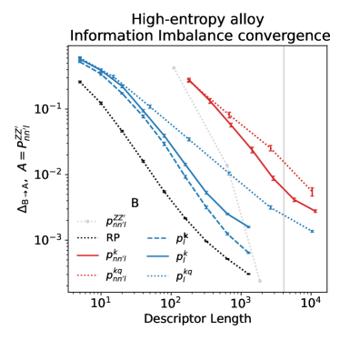
Figure 5: Convergence of the information imbalance, relative to the full power spectrum, for 1000 randomly chosen environments from liquid configurations in a high-entropy alloy dataset [42], S=5. Element and element-radial mixing are indicated using red and blue respectively. Fully coupled channels are indicated with a dotted line whilst uncoupled channels are indicated with a solid (or dashed) line. The black dotted line corresponds to a random projection of the full power spectrum whilst the grey dotted line corresponds to $p^{zz^{\prime}}_{nn^{\prime}l}$ computed using fewer basis functions (while keeping the $n_{\mathrm{max}}=2l_{\mathrm{max}}$ relation). Error bars show the standard error in the mean across 10 randomly chosen sets of weights and the vertical grey line indicates the length of the reference power spectrum, $n_{\mathrm{max}}=8,l_{\mathrm{max}}=4$.

A random projection [31, 30, 29] of $p^{zz^{\prime}}_{nn^{\prime}l}$ (black dashed) and the full power spectrum $p^{zz^{\prime}}_{nn^{\prime}l}$ itself but computed using fewer basis functions (grey dotted), which is a naive way of obtaining a shorter descriptor, are also included as references. Using the fully tensor-reduced power spectrum $p^{k}_{l}$ provides a performance only slighty inferior to random projection whilst avoiding constructing the full $p^{zz^{\prime}}_{nn^{\prime}l}$ as an intermediate step. Notably, using element-only mixing (red lines) is less efficient than creating a shorter descriptor simply by lowering the spatial resolution. Equivalent results for the revised MD17 [51] dataset and a single element phosphorous dataset [52] are shown below.

The SOAP descriptors were computed using a radial cut-off of 5 Å, $n_{\text{max}}=8$, $l_{\text{max}}=4$, $\sigma_{\text{at}}=0.5$ Åand the weight of the central atom set to 0. Shorter versions of the full power spectrum were computed using $n_{\text{max}}=2l_{\text{max}}$ for $l_{\text{max}}=1,2,3$.

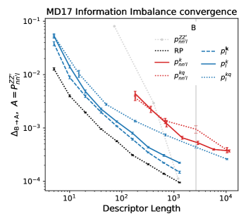
Figure 6: Convergence of the information imbalance with respect to descriptor length for 2000 carbon environments randomly selected from the revised MD17 dataset [51]. Element and element-radial mixing are indicated using red and blue respectively. Fully coupled channels are indicated with a dotted line whilst uncoupled channels are indicated with a solid (or dashed) line. The black dotted line is RP on the full power spectrum. Error bars show the standard error in the mean computed across 10 (20 for the red lines) randomly chosen sets of weights. The grey line corresponds to using the full power spectrum truncated using $n_{\mathrm{max}}=2l_{\mathrm{max}}$ for $l_{\mathrm{max}}=1,2,3$ where $l_{\mathrm{max}}$=4 is the reference used for all comparisons.

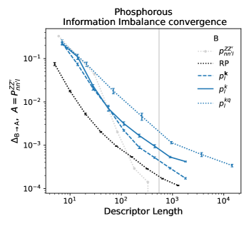
Figure 7: Convergence of the information imbalance, relative to the full SOAP power spectrum, is shown as a function of descriptor length for a dataset of P environments. The dataset was constructed by extracting 2000 environments from the training dataset of ref. [52] using CUR decomposition and the same SOAP parameters as the original work [50] were used. Fully coupled channels are indicated with a dotted line whilst uncoupled channels are indicated with a solid (or dashed) line. The black dotted line corresponds to a random projection of the full power spectrum. Error bars show the standard error in the mean computed across 10 randomly chosen sets of weights. The grey line corresponds to using the full power spectrum truncated using $n_{\mathrm{max}}=2l_{\mathrm{max}}$ for $l_{\mathrm{max}}=1,2,3,4,5$ where $l_{\mathrm{max}}=6$ is the reference used for all comparisons.

.5 SOAP-GAP energy convergence

The gap_fit command used to fit one of the models is shown below. The same parameters were used for all models with only the compress_file being changed. Note that for brevity only one example for each descriptor type has been included. For the actual models a two-body term was included for every pair of elements and a SOAP term was included for every element.

at_file=db_HEA_reduced.xyz core_param_file=pairpot.xml core_ip_args={IP Glue} sparse_jitter=1e-8
    gp_file=ER_diag_normal_K=64_2.xml rnd_seed=999 default_sigma={ 0.002 0.1 0.5 0.0}
gap={  {distance_2b cutoff=5.0 cutoff_transition_width=1.0 covariance_type=ard_se delta=10.0
    theta_uniform=1.0 n_sparse=20 Z1=42 Z2=42 add_species=F}  :
{soap_turbo species_Z={23 41 42 73 74} l_max=4 n_species=5 rcut_hard=5 rcut_soft=4 basis=poly3gauss
    scaling_mode=polynomial radial_enhancement=0 covariance_type=dot_product add_species=F delta=1.0
    n_sparse=2000 sparse_method=cur_points zeta=6 compress_file=ER_diag_KK_normal-8-4-5-64_2.dat
    central_index=1 alpha_max={8 8 8 8 8} atom_sigma_r={0.5 0.5 0.5 0.5 0.5}
    atom_sigma_t={0.5 0.5 0.5 0.5 0.5} atom_sigma_r_scaling={0.0 0.0 0.0 0.0 0.0}
    atom_sigma_t_scaling={0.0 0.0 0.0 0.0 0.0} amplitude_scaling={0.0 0.0 0.0 0.0 0.0}
    central_weight={1.0 1.0 1.0 1.0 1.0}}

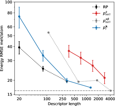
Figure 8: Convergence of energy errors on the test set as a function of descriptor length for various GAP models. The grey line is full SOAP using $n_{\mathrm{max}}=2l_{\mathrm{max}}$, for $l_{\mathrm{max}}=1,2,3,4$. The black dotted line is RP on the full power spectrum whilst the red and blue lines use a tensor-reduced features with element and element-radial mixing respectively. Error bars show the standard error in the mean, computed across 5 fits using independently chosen random weights.

.6 Details of the MACE models

The MACE models were trained on NVIDIA A100 GPU in single GPU training. The training, validation and test split of the HME21 dataset [47, 48] were used. The data set was reshuffled after each epoch. We constructed three seperate models, two with one layer and one with two layers. On all models, we used 256 uncoupled feature channels, $l_{max}=3$ and pass invariant messages $L_{max}=0$ only. For the model with random weights, we froze the weights of the initial chemical embedding. For all models, radial features are generated using 8 Bessel basis functions and a polynomial envelope for the cutoff with p = 5. The radial features are fed to an MLP of size [64, 64, 64, 1024], using SiLU nonlinearities on the outputs of the hidden layers. The readout function of the first layer is implemented as a simple linear transformation. For the model with the second layer, the readout function of the second layer is a single-layer MLP with 16 hidden dimensions. We used a cutoff of 6 Å. The standard weighted energy forces loss was used, with a weight of 1 on energies and a weight of 10 on forces [24].

Models were trained with AMSGrad variant of Adam, with default parameters of $\beta_{1}$ = 0.9, $\beta_{2}$ = 0.999, and $\epsilon$ = $10^{-8}$. We used a learning rate of 0.01 and a batch size of 5. The learning rate was reduced using an on-plateau scheduler based on the validation loss with a patience of 50 and a decay factor of 0.8.