Cooperative Self-Training for Multi-Target Adaptive Semantic Segmentation

Abstract

In this work we address multi-target domain adaptation (MTDA) in semantic segmentation, which consists in adapting a single model from an annotated source dataset to multiple unannotated target datasets that differ in their underlying data distributions. To address MTDA, we propose a self-training strategy that employs pseudo-labels to induce cooperation among multiple domain-specific classifiers. We employ feature stylization as an efficient way to generate image views that forms an integral part of self-training. Additionally, to prevent the network from overfitting to noisy pseudo-labels, we devise a rectification strategy that leverages the predictions from different classifiers to estimate the quality of pseudo-labels. Our extensive experiments on numerous settings, based on four different semantic segmentation datasets, validates the effectiveness of the proposed self-training strategy and shows that our method outperforms state-of-the-art MTDA approaches. Code available at: https://github.com/Mael-zys/CoaST.

1 Introduction

Semantic segmentation is a key task in computer vision that consists in learning to predict semantic labels for image pixels. Given its importance in many real world applications, segmentation is widely studied and significant progress has been made [1, 3, 4] in the supervised regime. Much of the recent success can be attributed to the availability of large, curated, and annotated datasets [7, 21, 45]. As obtaining labeled data in semantic segmentation is costly and tedious, pre-trained models are often deployed in test environments without fine-tuning. Unfortunately, these models fail when the test samples are drawn from a distribution which is different from the training distribution. This phenomenon is known as the domain shift [31] problem. To mitigate the domain-shift between the training (source) and test (target) distributions, Unsupervised Domain Adaptation (UDA) methods [8] have been proposed.

(a) Cooperative Self-training

(b) Cooperative Rectification

Figure 1: (a) Proposed method for Multi-Target Domain Adaptation (MTDA). Feature stylization is performed to favor consistency across classifiers via pseudo-labelling. Classifier consistency is used to estimate pseudo-label quality and rectify the training loss. (b) We show the uncertainty map estimated from an input image and used for loss rectification (dark blue for high confidence). We observe that low confidence regions often correspond to errors.

Although a vast majority of UDA methods have been proposed for semantic segmentation in the single source and single target setting, in practical applications the assumption of a single target domain easily becomes vacuous. It is because the real world is more complex and target data can come from varying and different data distributions. For e.g., in autonomous driving applications, the vehicle might encounter cloudy, rainy, and sunny weather conditions in a span of a very short journey. In such cases, it would require to switch among various adapted models specialized for a certain weather condition. To prevent cumbersome deployment operations one can instead train and deploy a single model for all the target environments, which is otherwise known as Multi-Target Domain Adaptation (MTDA). While in the context of object recognition MTDA has been explored in several works [6, 11, 23, 25, 38], it is heavily understudied for semantic segmentation, with just a handful of existing works [14, 16, 26]. The prior works are either sub-optimal at fully addressing the target-target alignment [26] or tackle it at a high computation overhead of explicit style-transfer [14, 16]. We argue that explicit interactions between a pair of target domains are essential in MTDA for minimizing the domain gap across target domains.

To this end, in this paper we present a novel MTDA framework for semantic segmentation that employs a self-training strategy based on pseudo-labeling to induce better synergy between different domains. Self-training is a widely used technique consisting in comparing different predictions obtained from a single image to impose consistency in network’s predictions. In our proposed method, illustrated in Fig. 1 (a), we use an original image from one target domain (in yellow box) as the view that generates the pseudo-label; while the second prediction is obtained with the very same target image but stylized with an image coming from a different target domain (in green box). Given this stylized feature, the network is then asked to predict the pseudo-label obtained from the original view. Unlike [14] we use implicit stylization that does not need any externally trained style-transfer network, making our self-training end-to-end. Self-training not only helps the network to improve the quality of representations but also helps in implicit alignment between target-target pairs due to cross-domain interactions.

While our proposed self-training is well-suited for MTDA, it can still be susceptible to noisy pseudo-labels. To prevent the network from overfitting to noisy pseudo-labels when the domain-shift is large, we devise a cross-domain cooperative rectification strategy that captures the disagreement in predictions from different classifiers. Specifically, our proposed method uses the predictions from multiple domain-specific classifiers to estimate the quality of pseudo-labels (see Fig. 1 (b)), which are then weighted accordingly during self-training. Thus, interactions between all the target domains are further leveraged with our proposed framework, which we call Co-operative Self-Training (CoaST) for MTDA.

Contributions. In summary, our contributions are three fold: (i) We propose a self-training approach for MTDA that synergistically combines pseudo-labeling and feature stylization to induce better cooperation between domains; (ii) To reduce the impact of noisy pseudo-labels in self-training, we propose cross-domain cooperative objective rectification that uses predictions from multiple domain-specific classifiers for better estimating the quality of pseudo-labels; and (iii) We conduct experiments on several standard MTDA benchmarks and advance the state-of-the-art performance by non-trivial margins.

2 Related Works

Our proposed method is most related to self-training and style-transfer, which we discuss in the following section.

Self-training for Domain Adaptation. Self-training in single-target domain adaptation (STDA) is a popular technique that involves generating pseudo-labels for the unlabeled target data and then iteratively training the model on the most confident labels. To that end, a plethora of UDA methods for semantic segmentation has been proposed [15, 17, 19, 36, 43, 44, 48] that use self-training due to its efficiency and simplicity. However, due to the characteristic error-prone nature of the pseudo-labeling strategy, the pseudo-labels cannot always be trusted and need a selection or correction mechanism. Most self-training methods differ in the manner in which the pseudo-labels are generated and selected. For instance, Zou et al.  [48] proposed a class-balanced self-training strategy and used spatial priors, whereas in  [41, 42] class-dependent centroids are employed to generate pseudo-labels. Most relevant to our approach are self-training methods [27, 43, 44] that rectify the pseudo-labels by measuring the uncertainty in predictions. Our proposed CoaST also derives inspirations from the STDA method  [44], but instead of ad-hoc auxiliary classifiers, we use different stylized versions of the same image and different target domain-specific classifiers, to compute the rectification weights. The majority of the STDA self-training methods do not trivially allow target-target interactions, which is very crucial for MTDA.

Style-Transfer for Domain Adaptation. Yet another popular technique in STDA that essentially relies on transferring style (appearance) to make a source domain image look like a target image or vice versa. Assuming the semantic content in the image remains unchanged in the stylization process, and hence the pixel labels, target-like source images can be used to train a model for the target domain. Thus, the main task becomes modeling the style and content in an image through an encoder-decoder-like network. In the context of STDA in semantic segmentation, Hoffman et al.  [13] proposed CyCADA, that incorporates cyclic reconstruction and semantic consistency to learn a classifier for the target data. Inspired by CyCADA a multitude of STDA methods [2, 5, 18, 20, 30, 37, 39, 47] have been proposed which use style-transfer in conjunction with other techniques. Learning a good encoder-decoder style-transfer network introduces additional training overheads and the success is greatly limited by the reconstruction quality. Alternatively, style-transfer can be performed in the feature space of the encoder without explicitly generating the stylized image [29, 46]. CrossNorm [29] explores this solution in the context of domain generalization to learn robust features. In CoaST, we adapt CrossNorm to our self-training mechanism by transferring style across target domains to induce better synergy.

Multi-target Domain Adaptation. MTDA for semantic segmentation is an under-explored field with just a handful of existing works [14, 16, 26]. For instance, Saporta et al.  [26] proposed an adversarial framework where source-target and target-target alignment is achieved through dedicated discriminators. They also introduced a multi-target knowledge transfer (MTKT) approach where knowledge distillation (KD) [12] is used to learn a domain-agnostic classifier from multiple domain-specific experts. On the other hand, the CCL [14] and ADAS [16] rely on explicit style-transfer to tackle MTDA in semantic segmentation. Much like other style-transfer based STDA methods, [16] uses an external network for explicitly transferring styles between domains. Instead, we rely on implicit style-transfer making our proposed CoaST easy to implement and end-to-end trainable. Additionally, we introduce a cooperative rectification technique which prevents over-fitting on imperfect pseudo-labels, making our method more robust. We empirically prove this effectiveness over [14, 16, 26] through numerous experiments.

3 Methods

In this section we formally define the MTDA task and then we present the details of our proposed Cooperative Self-Training (CoaST) framework.

3.1 Preliminaries

Figure 2: Illustration of the proposed CoaST approach in the case of two target domains. Domain-specific classifiers are distilled to learn a domain-agnostic classifier. Style-transfer is used in the encoder network to induce cooperation between the different classifiers and rectify the pseudo-labeling losses.

Problem Definition and Notations. In the multi-target domain adaptation (MTDA) task, we assume that we have at our disposal $N^{\mathtt{S}}$ labeled instances from a source domain data set $\mathcal{D}^{\mathtt{S}}=\{(\mathbf{x}^{\mathtt{S}}_{n},\mathbf{y}^{\mathtt{S}}_{n})\}^{N^{\mathtt{S}}}_{n=1}$ where $\mathbf{x}^{\mathtt{S}}\in\mathbb{R}^{H\times W\times 3}$ are input images with their corresponding one-hot ground truth labels $\mathbf{y}^{\mathtt{S}}\in\mathbb{R}^{H\times W\times K}$, assigned to each pixel in the $H\times W$ spatial grid belonging to one of the $K$ semantic classes. Moreover, there are a total of $M$ unlabeled target domains $\{\mathtt{T}_{1},\dots,\mathtt{T}_{M}\}$ where each target domain $\mathtt{T}_{i}$ comprises of an unlabeled data set $\mathcal{D}^{\mathtt{T}_{i}}=\{\mathbf{x}^{\mathtt{T}_{i}}_{n}\}^{N^{\mathtt{T}_{i}}}_{n=1}$, with $\mathbf{x}^{\mathtt{T}_{i}}\in\mathbb{R}^{H\times W\times 3}$ representing the target images and $N^{\mathtt{T}_{i}}$ being the number of unlabeled instances. Following standard MTDA protocols, we assume that the marginal distributions between every pair of available domains differ, under the constraint of underlying semantic concept remaining the same. The goal of MTDA is to learn a single network $f=C\circ\Phi$ using $\{\bigcup^{M}_{i=1}\mathcal{D}^{\mathtt{T}_{i}}\}\cup\mathcal{D}^{\mathtt{S}}$ that can segment samples from any target domain, where $C$ and $\phi$ are the classifier and the backbone encoder networks, respectively. While we consider that the domain information is known at training time, the domains labels of the images during inference are unknown.

Overall Framework. To address the MTDA, we operate in two stages. In the first stage we aim to learn target domain-specific classifiers with adversarial adaptation [32, 35] that aligns features between a given source-target domain pair. The first stage results in the network parameters that enable even better alignment in the subsequent stage. In this second stage, we adopt a pseudo-label based cooperative self-training strategy to further align the target domains. In particular, our proposed self-training strategy enforces consistency among the target domain-specific classifiers, allowing maximal interaction among the different target domains. Importantly, our cooperative training also incorporates a threshold-free rectification term that prevents overfitting to noisy pseudo-labels. Finally, we use knowledge distillation to distill all the learned information from domain-specific classifiers to a domain-agnostic classifier that can be used to segment a test image from any target domain, thereby alleviating the need for domain-id during inference.

Adversarial Warm-up. This marks the first stage, where we follow [26] for initializing our framework in order to obtain an encoder network $\Phi$ that is shared among all the target domains, and $M$ distinct target domain-specific classifiers $\{C^{\mathtt{T}_{i}}|\forall i\in\{1,\dots,M\}\}$. Concurrently, we also initialize $M$ target domain-specific discriminators $\{D^{\mathtt{T}_{i}}|\forall i\in\{1,\dots,M\}\}$ to learn a classifier that is invariant for a specific source-target pair. To recap, in adversarial warm-up stage the discriminator $D^{\mathtt{T}_{i}}$ is trained to distinguish between the source and target $\mathtt{T}_{i}$ predictions whereas the network $f^{\mathtt{T}_{i}}=C^{\mathtt{T}_{i}}\circ\Phi$ is trained to fool the $D^{\mathtt{T}_{i}}$. Note that unlike the original work in [10], the output from the classifier is given as an input to the domain discriminator [26, 32]. Additionally, for the source samples we employ the standard supervised cross-entropy loss, which is used to train every $f^{\mathtt{T}_{i}}$. Overall, for a given source-target pair $(\mathtt{S},\mathtt{T}_{i})$ the discriminator $D^{\mathtt{T}_{i}}$ is trained with the objective:

$$\begin{split}\mathcal{L}_{D^{\mathtt{T}_{i}}}=\mathcal{L}_{\mathrm{bce}}\big{(}D^{\mathtt{T}_{i}}(C^{\mathtt{T}_{i}}(\Phi(\mathbf{x}^{\mathtt{S}}))),1\big{)}+\\ \mathcal{L}_{\mathrm{bce}}\big{(}D^{\mathtt{T}_{i}}(C^{\mathtt{T}_{i}}(\Phi(\mathbf{x}^{\mathtt{T}_{i}}))),0\big{)}\end{split}$$ (1)

where $\mathcal{L}_{\mathrm{bce}}$ stands for the binary cross-entropy loss. Simultaneously, the network $f^{\mathtt{T}_{i}}$ is trained along with the source segmentation loss and adversarial loss as:

$$\begin{split}\mathcal{L}_{f^{\mathtt{T}_{i}}}=\mathcal{L}_{\mathrm{ce}}\big{(}C^{\mathtt{T}_{i}}(\Phi(\mathbf{x}^{\mathtt{S}})),\mathbf{y}^{\mathtt{S}}\big{)}+\\ \lambda_{adv}\mathcal{L}_{\mathrm{bce}}\big{(}D^{\mathtt{T}_{i}}(C^{\mathtt{T}_{i}}(\Phi(\mathbf{x}^{\mathtt{T}_{i}}))),1\big{)}\end{split}$$ (2)

where $\mathcal{L}_{\mathrm{ce}}$ is the supervised cross-entropy loss for the source data and $\lambda_{adv}$ is a hyperparameter to balance the losses. In the adversarial warm-up stage we alternatively minimize $\mathcal{L}_{\mathrm{D^{\mathtt{T}_{i}}}}$ and $\mathcal{L}_{\mathrm{f^{\mathtt{T}_{i}}}}$ for every source-target pairs.

3.2 Cooperative Self-Training (CoaST)

The goal of the second stage is to refine the image representation learned in the adversarial warm-up stage. We devise a self-training approach with the usage of pseudo-labels that iteratively improves the predictions of the model on the unlabeled data.

Pseudo-labelling. In our framework for the MTDA, we have $m$ specialized target domain-specific classifiers, with each classifier $C^{\mathtt{T}_{i}}$ trained to handle data coming from the corresponding domain $\mathtt{T}_{i}$. We exploit these specialized classifiers to generate pseudo-labels (PLs) for the target samples in their respective target domains. Specifically, given the $n$^th image $\mathbf{x}^{\mathtt{T}_{i}}_{n}$ from the target domain $i$, we use the network $f^{\mathtt{T}_{i}}$ to predict the segmentation map $[\hat{\mathbf{p}}^{\mathtt{T}_{i}}_{n}(\textbf{k})]_{\textbf{k}\in[H]\times[W]\times[K]}=C^{\mathtt{T}_{i}}(\Phi(\mathbf{x}^{\mathtt{T}_{i}}_{n}))$ and compute the pseudo-label as:

$$\hat{\mathbf{y}}^{\mathtt{T}_{i}}_{n}=\mathbf{e}_{k}\big{(}\operatornamewithlimits{argmax}_{k}[\hat{\mathbf{p}}^{\mathtt{T}_{i}}_{n}(\textbf{k})]_{\textbf{k}\in[H]\times[W]\times[K]}\big{)},$$ (3)

where $\mathbf{e}_{k}(.)$ denotes the one-hot encoding operator and $\hat{\mathbf{y}}^{\mathtt{T}_{i}}_{n}\in\mathbb{R}^{H\times W\times K}$. The PL is computed at the beginning of the second stage and is updated every $n_{b}$ iterations. This PL is then used to self-supervise the corresponding $f^{\mathtt{T}_{i}}$ network with a cross entropy loss:

$$\mathcal{L}_{\mathrm{pl}}=\mathcal{L}_{\mathrm{ce}}(\hat{\mathbf{p}}^{\mathtt{T}_{i}}_{n},\hat{\mathbf{y}}^{\mathtt{T}_{i}}_{n}),$$ (4)

However, this formulation suffers from two main issues. First, the PLs act only on the same domain-specific classifier $C^{\mathtt{T}_{i}}$ corresponding to the domain of input images. Hence, it does not induce any synergy between the different classifiers. Second, since the PLs can be noisy, using the pseudo-labeling objective in Eq. (4) can lead to detrimental behaviour. To address these two issues and further benefit from our PLs, we introduce a self-training technique that is realized by leveraging feature stylization [29].

Style-Transfer for Cooperative Self-Training. To benefit from the self-training objective in Eq. (4), one requires to obtain the predictions from a view $t(\mathbf{x}^{\mathtt{T}_{i}}_{n})$ and enforce its predictions to match with that of $\hat{\mathbf{y}}^{\mathtt{T}_{i}}_{n}$, where $t(.)$ is any stochastic transformation. Indeed, such a consistency-based training strategy has successfully been applied in the semi-supervised learning literature [28]. However, finding optimal transformations is not trivial and varies between data sets and even tasks. In this work, we resort to a data-driven transformation policy that is based on style-transfer [33]. Style-transfer consists in transferring the“style” (appearance) from one image to another. Concretely, in our case, the transformation $t(.)$ is a style-transfer operation that essentially applies the style of an image $\mathbf{x}^{\mathtt{T}_{j}}$ to the image $\mathbf{x}^{\mathtt{T}_{i}}$, where $i\neq j$. The style transformed image $\mathbf{x}^{\mathtt{T}_{i\to j}}$ can in essence be regarded as a virtual image that appears to come from $\mathtt{T}_{j}$ but having the content structure of $\mathtt{T}_{i}$. Therefore, for the $n$^th sample $\mathbf{x}^{\mathtt{T}_{i\to j}}$ we obtain the prediction from $f^{\mathtt{T}_{j}}$ and optimize it to be close to $\hat{\mathbf{y}}^{\mathtt{T}_{i}}_{n}$. In this way our PL from a given target domain-specific classifier can be used to supervise another domain-specific classifier, enforcing better consistency between pairs of target domains. Moreover, we thereafter show how style-transfer is instrumental in rectifying the objective in Eq. (4) according to an estimated confidence score. We now describe how we use style-transfer to improve self-training in the MTDA setting.

Style-transfer in the pixel space, with separately trained encoder-decoder network, has very recently been used for the MTDA work [16]. To avoid such costly, and often sub-optimal, image generation with the pixel-space style-transfer methods, we perform style-transfer in the intermediate feature space of the encoder network. In particular, we adapt cross normalization (CrossNorm) [29] in our MTDA setting and use it as a means of exchanging feature statistics, and hence style, across different domains. More precisely, our Cross-Domain Normalization (CrossDoNorm) performs style-transfer by exchanging style vectors between two target domain images, which are computed from the channel-wise mean and standard deviation of the features maps. Exchange of style vectors is deemed sufficient for style-transfer by prior works [33] who show that these statistics encode the image style and that style-transfer can be obtained through a simple re-normalization.

Given a pair of images ($\mathbf{x}^{\mathtt{T}_{i}},\mathbf{x}^{\mathtt{T}_{j}}$) from the target domains $\mathtt{T}_{i}$ and $\mathtt{T}_{j}$, we extract their corresponding features from the $l$^th layer of the encoder as $\mathbf{z}^{\mathtt{T}_{i}}_{l}=\Phi_{l}(\mathbf{x}^{\mathtt{T}_{i}})$ and $\mathbf{z}^{\mathtt{T}_{j}}_{l}=\Phi_{l}(\mathbf{x}^{\mathtt{T}_{j}})$. From these intermediate feature maps, we compute the corresponding channel-wise means ($\bm{\mu}^{\mathtt{T}_{i}}_{l},\bm{\mu}^{\mathtt{T}_{j}}_{l}$) and standard deviations ($\bm{\sigma}^{\mathtt{T}_{i}}_{l},\bm{\sigma}^{\mathtt{T}_{j}}_{l}$), such that $\bm{\mu}_{l}\in\mathbb{R}^{k}$ and $\bm{\sigma}_{l}\in\mathbb{R}^{k}$ with $k$ being the number of channels in the layer $l$. For instance, CrossDoNorm first standardizes the features with its own channel-wise statistics, e.g., ($\bm{\mu}^{\mathtt{T}_{i}}_{l},\bm{\sigma}^{\mathtt{T}_{i}}_{l}$) for $\mathbf{z}^{\mathtt{T}_{i}}_{l}$, and then re-normalizes with the statistics from the other domain ($\bm{\mu}^{\mathtt{T}_{j}}_{l},\bm{\sigma}^{\mathtt{T}_{j}}_{l}$) to obtain stylized features $\mathbf{z}^{\mathtt{T}_{i\to j}}_{l}$. The CrossDoNorm can be done symmetrically resulting into stylized features that are computed as:

$$\begin{split}\mathbf{z}^{\mathtt{T}_{i\to j}}_{l}=\bm{\sigma}^{\mathtt{T}_{j}}_{l}\frac{\mathbf{z}^{\mathtt{T}_{i}}_{l}-\bm{\mu}^{\mathtt{T}_{i}}_{l}}{\bm{\sigma}^{\mathtt{T}_{i}}_{l}}+\bm{\mu}^{\mathtt{T}_{j}}_{l}\\ \mathbf{z}^{\mathtt{T}_{j\to i}}_{l}=\bm{\sigma}^{\mathtt{T}_{i}}_{l}\frac{\mathbf{z}^{\mathtt{T}_{j}}_{l}-\bm{\mu}^{\mathtt{T}_{j}}_{l}}{\bm{\sigma}^{\mathtt{T}_{j}}_{l}}+\bm{\mu}^{\mathtt{T}_{i}}_{l}\end{split}$$ (5)

Our CrossDoNorm can ideally perform feature stylization at multiple layers in the encoder network. Next, the above computed stylized feature $\mathbf{z}^{\mathtt{T}_{i\to j}}_{l}$ is then given as input to the subsequent layers of the network, with the final prediction map $\hat{\mathbf{p}}^{\mathtt{T}_{i\to j}}$ obtained from the classifier $C^{\mathtt{T}_{j}}$. With the PL $\hat{\mathbf{y}}^{\mathtt{T}_{i}}$ generated from $\mathbf{z}^{\mathtt{T}_{i}}_{l}$ by the original domain classifier $C^{\mathtt{T}_{i}}$, the other classifier $C^{\mathtt{T}_{j}}$, along with the encoder $\Phi$, is then trained in a supervised manner:

$$\begin{split}\mathcal{L}_{\mathrm{pl}}^{\mathrm{sty}}(\mathbf{x}^{\mathtt{T}_{i}},\mathbf{x}^{\mathtt{T}_{j}})=\mathcal{L}_{\mathrm{ce}}(\hat{\mathbf{p}}^{\mathtt{T}_{i\to j}},\hat{\mathbf{y}}^{\mathtt{T}_{i}})\\ \mathcal{L}_{\mathrm{pl}}^{\mathrm{sty}}(\mathbf{x}^{\mathtt{T}_{j}},\mathbf{x}^{\mathtt{T}_{i}})=\mathcal{L}_{\mathrm{ce}}(\hat{\mathbf{p}}^{\mathtt{T}_{j\to i}},\hat{\mathbf{y}}^{\mathtt{T}_{j}})\end{split}$$ (6)

Since it has been shown in the literature that training with soft-labels improves the learning ability of the network [12], we use a soft-version of the $\mathcal{L}^{\mathrm{sty}}_{\mathrm{pl}}$ loss described in Eq. (6). In other words, we further enforce consistency in predictions between two domain-specific classifiers by optimizing the KL-divergence objective between the cross-domain stylized prediction $\hat{\mathbf{p}}^{\mathtt{T}_{i\to j}}$ and the original target domain prediction $\hat{\mathbf{p}}^{\mathtt{T}_{i}}$ instead of PLs as:

$$\mathcal{L}_{\mathrm{cst}}(\mathbf{x}^{\mathtt{T}_{i}},\mathbf{x}^{\mathtt{T}_{j}})=\mathcal{L}_{\mathrm{kl}}(\hat{\mathbf{p}}^{\mathtt{T}_{i\to j}},\hat{\mathbf{p}}^{\mathtt{T}_{i}})$$ (7)

Additionally, our CrossDoNorm also acts as an implicit data augmentation method in the feature space. As the style information is mainly manifested in the low level features of the encoder, to prevent over-regularization we only apply the CrossDoNorm in the initial layers of the encoder.

Cooperative Objective Rectification. The PLs generated during the refinement process can be very noisy due to domain-shift, leading to degradation of representations. To tackle this shortcoming of self-training, we propose our cooperative objective rectification method that takes into account the uncertainty in the model predictions. This uncertainty in predictions for a given sample $\mathbf{x}^{\mathtt{T}_{i}}_{n}$ is measured by combining the predictions obtained from all the target domain classifiers. More precisely, considering $\mathbf{x}^{\mathtt{T}_{i}}_{n}$, we compute the consistency scores between the prediction from the $C^{\mathtt{T}_{i}}$ and the predictions from the other domain-specific classifiers on the stylized features of $\mathbf{x}^{\mathtt{T}_{i}}_{n}$. Following [44], we use the KL-divergence between a pair of predictions as a measure of consistency. Lower the consistency, less reliable is the corresponding PL. Finally, this consistency score is then used as a weight to re-weight the self-training loss introduced in the Eq. (4). The rectified self-training loss corresponding to Eq. (4) is given as:

$$\bar{\mathcal{L}}_{\mathrm{pl}}(\mathbf{x}^{\mathtt{T}_{i}})=w_{i}\mathcal{L}_{\mathrm{ce}}(\hat{\mathbf{p}}^{\mathtt{T}_{i}},\hat{\mathbf{y}}^{\mathtt{T}_{i}})$$ (8)

where the weight value $w_{i}$ is the averaged consistency scores obtained with the predictions between $C^{\mathtt{T}_{i}}$ and the rest of the classifiers {$C^{\mathtt{T}_{1}},\dots,C^{\mathtt{T}_{M}}$}$\setminus C^{\mathtt{T}_{i}}$ as:

$$w_{i}=\frac{1}{M-1}\sum_{j=1,j\neq i}^{M}\exp{(-\mathcal{L}_{\mathrm{kl}}(\hat{\mathbf{p}}^{\mathtt{T}_{i}},\hat{\mathbf{p}}^{\mathtt{T}_{i\to j}})})$$ (9)

where the exponential function exp($\cdot$) is used here to map the KL divergence that range in $[0,+\infty[$ to weights values in ]0,1]. Contrary to [44] our uncertainty score is obtained by considering the predictions from all classifier pairs, against just using a single pair of classifiers. Also, different from many pseudo-labeling approaches described in Sec. 2, our re-weighting formulation is not based on thresholding and therefore avoids manual hyperparameter tuning. Similarly, the cross-domain pseudo labeling losses introduced in Eq. (6) are rectified as:

$$\begin{split}\bar{\mathcal{L}}^{\mathrm{sty}}_{\mathrm{pl}}(\mathbf{x}^{\mathtt{T}_{i}},\mathbf{x}^{\mathtt{T}_{j}})=w_{i}\mathcal{L}_{\mathrm{ce}}(\hat{\mathbf{p}}^{\mathtt{T}_{i\to j}},\hat{\mathbf{y}}^{\mathtt{T}_{i}})\\ \bar{\mathcal{L}}^{\mathrm{sty}}_{\mathrm{pl}}(\mathbf{x}^{\mathtt{T}_{j}},\mathbf{x}^{\mathtt{T}_{i}})=w_{j}\mathcal{L}_{\mathrm{ce}}(\hat{\mathbf{p}}^{\mathtt{T}_{j\to i}},\hat{\mathbf{y}}^{\mathtt{T}_{j}})\end{split}$$ (10)

Knowledge Distillation. As our end goal is to be able to predict test samples coming from any target domain, we also learn an additional domain-agnostic classifier $C^{\mathrm{A}}$. We use the source samples to train $C^{\mathrm{A}}$ in addition to the supervised segmentation objective given in Eq. (2) as:

$$\begin{split}\mathcal{L}_{\mathrm{seg}}=\sum_{i=1}^{M}\mathcal{L}_{\mathrm{ce}}(C^{\mathtt{T}_{i}}(\Phi(\mathbf{x}^{\mathtt{S}})),\mathbf{y}^{\mathtt{S}})\\ +\mathcal{L}_{\mathrm{ce}}(C^{\mathrm{A}}(\Phi(\mathbf{x}^{\mathtt{S}})),\mathbf{y}^{\mathtt{S}})\end{split}$$ (11)

In order to distill the information learned by the domain-specific classifiers $C^{\mathtt{T}_{i}}$ into the domain-agnostic classifier $C^{\mathrm{A}}$ we use knowledge distillation (KD) as in [14, 26]. For every target domain sample, we enforce consistency between the prediction from the corresponding domain-specific classifier and the domain-agnostic one using the KL divergence. The KD loss for a given $\mathtt{T}_{i}$ domain is given as:

$$\mathcal{L}_{\mathrm{kd}}=\mathcal{L}_{\mathrm{kl}}(C^{\mathrm{A}}(\Phi(\mathbf{x}^{\mathtt{T}_{i}})),\hat{\mathbf{y}}^{\mathtt{T}_{i}})$$ (12)

where only the weights of the $C^{\mathrm{A}}$ is only updated during the optimization of Eqn. 12. We use the domain-agnostic classifier $C^{\mathrm{A}}$ during inference.

Overall Training. The final objective to train our proposed CoaST is given by summing all the unary and pairwise losses previously described:

$$\begin{split}&\mathcal{L}_{\mathrm{\emph{CoaST}}}=\sum_{(\mathbf{x}^{\mathtt{S}},\mathbf{y}^{\mathtt{S}})\in\mathcal{D}^{\mathtt{S}}}\mathcal{L}_{\mathrm{seg}}(\mathbf{x}^{\mathtt{S}},\mathbf{y}^{\mathtt{S}})+\\ &\sum_{i=1}^{M}\sum_{\mathbf{x}^{\mathtt{T}_{i}}\in\mathcal{D}^{\mathtt{T}_{i}}}\Big{[}\frac{1}{M}\mathcal{L}_{\mathrm{kd}}(\mathbf{x}^{\mathtt{T}_{i}})+\bar{\mathcal{L}}_{\mathrm{pl}}(\mathbf{x}^{\mathtt{T}_{i}})+\\ &\frac{1}{M-1}\sum_{\begin{subarray}{c}j=1\\ j\neq i\end{subarray}}^{M}\sum_{\mathbf{x}^{\mathtt{T}_{j}}\in\mathcal{D}^{\mathtt{T}_{j}}}\bar{\mathcal{L}}_{\mathrm{pl}}^{\mathrm{sty}}(\mathbf{x}^{\mathtt{T}_{i}},\mathbf{x}^{\mathtt{T}_{j}})+\mathcal{L}_{\mathrm{cst}}(\mathbf{x}^{\mathtt{T}_{i}},\mathbf{x}^{\mathtt{T}_{j}})\Big{]}\end{split}$$ (13)

Note that, the KD loss and pairwise losses are normalized by $M$ and $M-1$ to preserve the source-target balance when varying the number of target domains.

4 Experiments

4.1 Experimental set-up

Datasets. We conduct experiments on two standard benchmarks for MTDA in semantic segmentation. These two benchmarks have been derived from four semantic segmentation datasets, namely the synthetic GTA5 [24] and the real world Cityscapes [7], Mapillary [21] and IDD [34]. Note that the datasets are varying in size as in the Mapillary is six times bigger than the Cityscapes, and thrice as big as the IDD. More details can be found in the supplement.

Benchmarks. The benchmarks for MTDA in semantic segmentation differ in the way the class labels are mapped across the datasets. They are: (i) the 7-classes benchmark, introduced in [26], which considers 7 classes and down-samples the images to a resolution of $640\times 320$ both for training and evaluation; and (ii) the 19-classes benchmark, introduced in [14], which operates at higher resolution of $1024\times 512$. Both benchmarks use several combinations of the four datasets to create four Synthetic to Real scenarios and one Real to Real scenario.

Metrics. We report the standard intersection over union (IoU) for every class and the mean-IoU (mIoU) for each target domain. Whereas, to obtain a single overall score in the MTDA, we average the mIoU across all the target domains.

Baselines. In our experiments, we compare with the state-of-the-art methods: Multi-Target Knowledge Transfer (MTKT) [26], Collaborative Consistency Learning (CCL) [14] and A Direct Adaptation Strategy (ADAS) [16]. We compare with these methods on the settings adopted in the corresponding papers: 7-classes for MTKT and 19-classes for CCL. We also include an approach, introduced in [26] and referred to as Multi-Discriminator, where a single classifier is trained using multiple domain-specific discriminator. In addition, we follow [14, 26] and include two baselines based on a single-target domain adaptation method. In Individual, an adversarial approach [35] is trained separately on every target dataset. At inference time, the target images are tested by the corresponding domain-specific model. In Data combination, we treat the union of all the target domains as a single target domain. For these two baselines, we report the results provided in [14, 26].

Implementation Details. To be fairly comparable, we adopt the very same network architecture as in the baseline [26], except we use the modified version of ResNet101 based DeepLab-V2 [3] that contains dropout layers [41, 44]. Due to lack of space we report the rest of the implementation details in the supplement.

GTA5 $\rightarrow$ Cityscapes + IDD
Method	Target	flat	constr	object	nature	sky	human	vehicle	mIoU	Avg.
Individual [35]	C	93.5	80.5	26.0	78.5	78.5	55.1	76.4	69.8	67.5
	I	91.2	53.1	16.0	78.2	90.7	47.9	78.9	65.1
Data Comb. [35]	C	93.9	80.2	26.2	79.0	80.5	52.5	78.0	70.0	67.4
	I	91.8	54.5	14.4	76.8	90.3	47.5	78.3	64.8
Multi-Dis [26]	C	94.3	80.7	20.9	79.3	82.6	48.5	76.2	68.9	67.3
	I	92.3	55.0	12.2	77.7	92.4	51.0	80.2	65.7
MTKT [26]	C	94.5	82.0	23.7	80.1	84.0	51.0	77.6	70.4	68.2
	I	91.4	56.6	13.2	77.3	91.4	51.4	79.9	65.9
ADAS [16]($1024\times 512$)	C	95.1	82.6	39.8	84.6	81.2	63.6	80.7	75.4	71.2
	I	90.5	63.0	22.2	73.7	87.9	54.3	76.9	66.9
CoaST (Ours)	C	94.7	82.9	25.4	82.2	88.2	54.4	80.5	72.6	71.3
	I	94.2	61.5	20.0	82.7	93.4	55.5	82.6	70.0

Table 1: Comparison with State-of-the-art on the 7-classes benchmark using the GTA5 $\rightarrow$ Cityscapes + IDD configuration.

GTA5 $\rightarrow$ Cityscapes + IDD
Method	Target	road	sidewalk	building	walk	fence	pole	light	sign	veg	terrain	sky	person	rider	car	truck	bus	train	motor	bike	mIoU	Avg.
Individual [35]	C	88.8	23.8	81.5	27.7	27.3	31.7	33.2	22.9	83.1	27.0	76.4	58.5	28.9	84.3	30.0	36.8	0.3	27.7	33.1	43.3	43.5
	I	94.1	24.4	66.1	31.3	22.0	25.4	9.3	26.7	80.0	31.4	93.5	48.7	43.8	71.4	49.4	28.5	0	48.7	34.3	43.6
Data Comb.[35]	C	86.1	32.0	79.8	24.3	22.3	28.5	27.9	14.3	85.1	29.8	79.9	56.1	20.5	77.7	34.4	35.2	0.7	18.2	13.1	40.3	41.2
	I	92.8	23.4	60.9	25.8	23.4	24.1	8.6	32.2	77.5	26.8	92.3	48.0	41.0	74.4	48.4	17.7	0	52.5	28.2	42.0
CCL [14]	C	90.3	34.0	82.5	26.2	26.6	33.6	35.4	21.5	84.7	39.8	81.1	58.4	25.8	84.5	31.4	45.4	0	29.9	24.7	45.0	45.5
	I	95.0	30.5	65.6	29.4	23.4	29.2	12.0	37.8	77.3	31.3	91.9	52.4	48.3	74.9	50.1	36.6	0	56.1	32.4	46.0
ADAS [16]	C	-	-	-	-	-	-	-	-	-	-	-	-	-	-	-	-	-	-	-	45.8	46.1
	I	-	-	-	-	-	-	-	-	-	-	-	-	-	-	-	-	-	-	-	46.3
CoaST (Ours)	C	81.7	38.3	71.0	33.3	30.7	35.1	38.2	37.6	86.4	46.9	81.9	63.4	27.4	84.5	29.4	45.6	0.3	32.6	31.3	47.1	48.2
	I	85.7	36.1	65.1	33.2	23.7	32.8	19.0	62.9	82.5	29.5	91.8	52.1	55.3	83.4	62.9	46.1	0	55.5	18.5	49.3

Table 2: Comparison with State-of-the-art on the 19-classes benchmark using the GTA5 $\rightarrow$ Cityscapes + IDD configuration.

4.2 Comparison with State-of-the-art: Syn to Real

Quantitative Comparison. We provide a detailed comparison with state-of-the-art on the 7-classes benchmark using the GTA5 to Cityscapes and IDD setting. Results are reported in Tab. 1. Overall, we can observe that our method outperforms all the other baselines. In terms of average mIoU, CoaST outperforms MTKT with a $3.1\%$ margin. This gain is remarkable considering that MTKT improves the Individual baseline trained on Cityscapes by only $0.7\%$. Besides, CoaST outperforms ADAS by $0.1\%$ even though ADAS use a higer image resolution than CoaST and the other baselines. We can observe gains with respect to MTKT in both small objects such as human ($54.4\%$ vs $51.0\%$ on Cityscapes) and background classes such as sky ($88.2\%$ vs $84.0\%$ on Cityscapes). One noticeable point is that the IDD dataset seems more challenging since Individual obtains lower performance on this dataset. Similarly, the Multi-Dis, MTKT and ADAS obtain mIoUs of $65.7\%$, $65.9\%$ and $66.9\%$ respectively which are much lower than on Cityscapes ($68.9\%$, $70.4\%$ and $75.4\%$). However, with CoaST, which uses consistency training and cooperative objective rectification, we improve MTKT and ADAS performance by $4.1\%$ and $3.1\%$ obtaining a mIoU score of $70.0\%$.

We now provide experimental results on the 19-classes benchmark using the same GTA5 to Cityscapes and IDD setting. Results are reported in Tab. 2. First, we observe that all methods have lower scores compared to the 7-classes since the high number of classes makes the task more difficult. Nevertheless, we observe that CoaST outperforms all the other approaches on almost all the classes and domains. Compared to CCL and ADAS, we observe that CoaST obtains better average mIoU ($+2.7\%$ and $+2.1\%$ respectively) and that the gain is mostly explained by better performances on difficult classes such as fence or sign and bus that largely compensate the drop on the road class.

Qualitative Comparison. Fig. 3 shows a qualitative comparison with MTKT on the 7-classes benchmark when adapting from GTA5 to Cityscapes and IDD. From these visualizations, we can see that CoaST segment better small objects such as ’human’ or ’object’ classes. This difference is especially clear on the IDD dataset.

Summary of all the Settings. To complete this evaluation in the Synthetic to Real scenario, we report in Tab. 3 the average mIoU considering all the possible target configurations on the 19-classes benchmark. Results on the 7-classes benchmark are reported in supplement. For the 19-classes benchmarks, the proposed method is compared with the best respective competitor. In short, we observe that CoaST obtains the best performance in all configurations and on all the domains. These experiments demonstrate the robustness of our approach.

Target			method	mIoU			mIoU
C	I	M		C	I	M	Avg.
$\surd$	$\surd$	-	CCL [14]	45.0	46.0	-	45.5
			ADAS [16]	45.8	46.3	-	46.1
			CoaST (Ours)	47.1	49.3	-	48.2
$\surd$	-	$\surd$	CCL [14]	45.1	-	48.8	47.0
			ADAS [16]	45.8	-	49.2	47.5
			CoaST (Ours)	47.9	-	51.8	49.9
-	$\surd$	$\surd$	CCL [14]	-	44.5	46.4	45.5
			ADAS [16]	-	46.1	47.6	46.9
			CoaST (Ours)	-	49.5	51.6	50.6
$\surd$	$\surd$	$\surd$	CCL [14]	46.7	47.0	49.9	47.9
			ADAS [16]	46.9	47.7	51.1	48.6
			CoaST (Ours)	47.2	48.7	51.4	49.1

Table 3: Summary of performances obtained on the 19-classes benchmark. Cityscapes, IDD and Mapillary are referred to as C, I and M respectively. We report the mIoU averaged over the target domains.

Model	Adv.	Self-Tr.	CrossDoNorm	$\mathcal{L}_{cst}$	Rec.	C	I	Avg.
MTKT* [26]	$\surd$					67.3	64.3	65.8
(i)		$\surd$				65.6	63.2	64.4
(ii)		$\surd$	$\surd$			69.2	67.4	68.4
(iii)		$\surd$	$\surd$	$\surd$		70.2	67.5	68.9
(iv)		$\surd$	$\surd$		$\surd$	72.1	69.9	71.0
(v)		$\surd$	$\surd$	$\surd$	$\surd$	72.6	70.0	71.3

Table 4: Ablation study of the proposed method on 7-classes benchmark, in GTA5 $\rightarrow$ Cityscapes + IDD configuration.

Rectification	C	I	Avg.
Without	70.2	67.5	68.9
Drop-Out-based [9]	70.7	68.7	69.7
Auxiliary network [44]	69.8	68.7	69.3
Cooperative (ours)	72.6	70.0	71.3

Table 5: Ablation study on the GTA5 $\rightarrow$ Cityscapes + IDD configuration: Rectification strategy

Cityscapes				IDD
Input	GT	MTKT	CoaST (Ours)	Input	GT	MTKT	CoaST (Ours)

Figure 3: Qualitative comparison with MTKT on the 7-classes benchmark and in the GTA5 to Cityscapes and IDD setting.

4.3 Ablation Study

To illustrate the impact of the proposed cooperative self-training and rectification, we present a detailed ablation study. We present several variants of CoaST. First, we employ our architecture but with the adversarial training scheme of MTKT [26]. The goal of this variant is to show that our performance gain is not due to our slight architectural change in the classifiers. This variant is referred to as MTKT*. Then we ablate different parts of our model: (i) uses a simple Self-training with pseudo-labeling without cross domain interactions. (ii) performs style-transfer and employs the cross-domain pseudo-label loss $\mathcal{L}_{pl}^{sty}$ in Eq. (10). (iii) adds the consistency loss given in Eq. (7). (iv) employs our rectified loss but does not use the consistency loss. Finally, (v) denotes our full models.

The lower performance of MTKT* demonstrates that the higher performance of CoaST is not due to the use of a different classifier. Then, we can observe that (i) under-performs MTKT* showing that naively replacing adversarial training by self-training does not work well. Adding CrossDoNorm in (ii) results in a $4\%$ gain that is further increased when a consistency loss is added (see (iii)). Cooperation between domains can be also obtained by introducing cross-domain rectification (see (iv)) but the experiments show that combining both consistency and pseudo label rectification leads to the best performance.

To complete this ablation study, we evaluate different solutions to assess the rectification weights $w_{i}$ in the same setting as Tab. 5. We consider different possibilities. Cooperative cross domain rectification can be replaced by the consistency between predictions obtained with multiple drop-out sampling [9]. An auxiliary network can also be employed as in [44] to estimate the uncertainty. Average mIoUs are reported in Tab. 5 with these different rectification approaches. We observe our approach which benefits from the multiple target domains, achieves a $2.4\%$ gain, which demonstrates that leveraging the multiple target domains is essential to achieve robust pseudo-labeling.

5 Conclusion

We presented CoaST, a new method for multi-target domain adaptation in semantic segmentation. We introduced a self-training strategy that uses pseudo-labels in conjunction with style-transfer to favor consistency between classifiers. Besides, we employed consistency between the predictions from the different classifiers as an uncertainty measure allowing better use of the pseudo-labels. We conducted experiments in two benchmarks and several settings and demonstrated that the proposed method outperforms state-of-the-art approaches.

Acknowledgements. This paper has been partially supported by the French National Research Agency (ANR) in the framework of its Technological Research JCJC pro- gram (Odace, project ANR-20-CE23-0027), NSFC (62176155), Shanghai Municipal Science and Technology Major Project (2021SHZDZX0102), the EU ISFP PROTECTOR (101034216) project and the EU H2020 MARVEL (957337) project.

Supplementary Material for
Cooperative Self-Training for Multi-Target
         Adaptive Semantic Segmentation

The supplementary material is organized as follows: Sec. A summarizes the notations used. Sec. B describes the experimental details of our work. Sec. C reports the ablation study on hyperparameter sensitivity. Sec. D lists detailed quantitative comparisons on various configurations.

Appendix A Notation

We summarize in Table A1 the notation used throughout the paper:

Notation	Description
$\mathcal{D}^{\mathtt{S}}=\{(\mathbf{x}^{\mathtt{S}}_{n},\mathbf{y}^{\mathtt{S}}_{n})\}^{N^{\mathtt{S}}}_{n=1}$	Source data set
$\mathcal{D}^{\mathtt{T}_{i}}=\{\mathbf{x}^{\mathtt{T}_{i}}_{n}\}^{N^{\mathtt{T}_{i}}}_{n=1}$	$i$th target data set
$\mathbf{x}^{\mathtt{S}}\in\mathbb{R}^{H\times W\times 3}$	Source inputs
$\mathbf{y}^{\mathtt{S}}\in\mathbb{R}^{H\times W\times K}$	Source labels
$\mathbf{x}^{\mathtt{T}_{i}}\in\mathbb{R}^{H\times W\times 3}$	Inputs from $i$th target domain
$f$	Model function
$\Phi$	Encoder network
$C^{\mathtt{T}_{i}}$	$i$th target domain-specific classifier
$C^{A}$	Domain-agnostic classifier
$D^{\mathtt{T}_{i}}$	$i$th target domain-specific discriminator
$\hat{\mathbf{p}}^{\mathtt{T}_{i}}\in\mathbb{R}^{H\times W\times K}$	Prediction from $i$th target domain-specific classifier
$\mathbf{e}_{k}$	One-hot encoding operator
$\hat{\mathbf{y}}^{\mathtt{T}_{i}}\in\mathbb{R}^{H\times W}$	Pseudo-label for $i$th target domain sample
$\mathbf{z}^{\mathtt{T}_{i}}_{l}=\Phi_{l}(\mathbf{x}^{\mathtt{T}_{i}})$	Latent feature of $\mathbf{x}^{\mathtt{T}_{i}}$ at $l$th layer in $\Phi$th layer
$\bm{\mu}^{\mathtt{T}_{i}},\bm{\sigma}^{\mathtt{T}_{i}}$	Style vectors (channel-wise mean and standard deviation) for $i$th target domain input $\mathbf{x}^{\mathtt{T}_{i}}$
$\mathbf{z}^{\mathtt{T}_{i\to j}}_{l}$	Latent stylized feature of $\mathbf{x}^{\mathtt{T}_{i}}$ with content from $\mathbf{x}^{\mathtt{T}_{i}}$ and style from $\mathbf{x}^{\mathtt{T}_{j}}$
$w_{i}$	Averaged rectification weight for the sample $\mathbf{x}^{\mathtt{T}_{i}}$

Table A1: Notation used throughout the paper

Appendix B Experimental Details

Datasets. We evaluate our method on two benchmarks previously used in the literature. These benchmarks are based on four datasets:

• GTA5 [24] is collected from the video game GTA5. The dataset contains 24966 labeled images in total where the image resolution is 1914 $\times$ 1052. The synthetic nature of this dataset makes it very relevant for domain adaptation experiments.

• Cityscapes [7] is a large-scale dataset that has 2975 training and 500 validation labeled images collected mainly in German cities.

• Mapillary [21] contains 18000 training and 2000 validation high-resolution images collected from all over the world. Compared to Cityscapes, this dataset is more diverse.

• IDD [34] is collected on Indian roads and it has 6993 and 981 finely annotated images in training and validation sets respectively. IDD is very challenging since India cities visually differ from the cities depicted in the other datasets.

Implementation details. In the warm-up stage, we employ the hyper-parameters as [26] except that we extend the warm-up stage from 20K to 60K iterations to get better initial pseudo-labels for the self-training stage. In the second stage, we use Stochastic Gradient Descent optimizer with learning rate $1.0\times 10^{-4}$ to train the model for another 60K iterations. In all the experiments in the 7-classes and 19-classes settings, we use random crop of size $320\times 160$ and $512\times 256$ respectively to accelerate the training. In the second stage, we use strong data-augmentation and update the pseudo-labels every 10K iterations.

Appendix C Ablation Study of Hyperparameters

In the final objective of our proposed CoaST, we weigh all the constituent losses and set other hyperparameters with a value that equals to 1. This disposes off the need to have a target validation set, which indeed is not available for any UDA setting. Nevertheless, below we study the sensitivity of CoaST with respect to two hyperparameters over ranges of possible values.

Ratio of Pair-wise Losses. We perform an ablation study on the weighing hyperparameter $\lambda$ that weighs the pair-wise losses: consistency loss $\mathcal{L}_{\mathrm{cst}}$ and the rectified segmentation losses $\bar{\mathcal{L}}^{\mathrm{sty}}_{\mathrm{pl}}$. The weighted training objective of our CoaST, first introduced in Eqn. LABEL:eqn:final-objective of the main paper, is written as:

$$\begin{split}\mathcal{L}_{\mathrm{\emph{CoaST}}}=\sum_{(\mathbf{x}^{\mathtt{S}},\mathbf{y}^{\mathtt{S}})\in\mathcal{D}^{\mathtt{S}}}\mathcal{L}_{\mathrm{seg}}(\mathbf{x}^{\mathtt{S}},\mathbf{y}^{\mathtt{S}})\\ +\sum_{i=1}^{M}\sum_{\mathbf{x}^{\mathtt{T}_{i}}\in\mathcal{D}^{\mathtt{T}_{i}}}\Big{[}\frac{1}{M}\mathcal{L}_{\mathrm{kd}}(\mathbf{x}^{\mathtt{T}_{i}})+\bar{\mathcal{L}}_{\mathrm{pl}}(\mathbf{x}^{\mathtt{T}_{i}})\\ +{\lambda}\frac{1}{M-1}\sum_{\begin{subarray}{c}j=1\\ j\neq i\end{subarray}}^{M}\sum_{\mathbf{x}^{\mathtt{T}_{j}}\in\mathcal{D}^{\mathtt{T}_{j}}}\big{(}\bar{\mathcal{L}}_{\mathrm{pl}}^{\mathrm{sty}}(\mathbf{x}^{\mathtt{T}_{i}},\mathbf{x}^{\mathtt{T}_{j}})\\ +\mathcal{L}_{\mathrm{cst}}(\mathbf{x}^{\mathtt{T}_{i}},\mathbf{x}^{\mathtt{T}_{j}})\big{)}\Big{]}\end{split}$$ (A1)

From the Fig. A1 (left), we can see that, the mIoU remains fairly stable over a wide operating window of $\lambda$. The performance starts to drop only when we increase the value of $\lambda$ to large values. This is reasonable because when $\lambda=10$, the $\mathcal{L}_{\mathrm{cst}}$ and the $\bar{\mathcal{L}}^{\mathrm{sty}}_{\mathrm{pl}}$ starts to dominate the other losses in Eqn A1. We observe a well-behaved training dynamics when we set the value of $\lambda$ to standard value of 1, or $\log\lambda=0$.

Temperature. The rectification weight described in the Eqn. 9 of the main paper is obtained by applying an exponential operation on the consistency score. To recap, the exp(.) function is used to bound the KL-divergence consistency score between ]0,1], which otherwise is unbounded. The rectification weight can be regulated by using a temperature hyperparameter $\gamma$, that controls the steepness of the exp(.) curve. In other words, higher the value of $\gamma$, more quickly the curve goes to zero, and vice-versa. The rectification weight which is a function of $\gamma$ is given as:

$$w_{i}=\frac{1}{M-1}\sum_{j=1,j\neq i}^{M}\exp{(-{\gamma}\mathcal{L}_{\mathrm{kl}}(\hat{\mathbf{p}}^{\mathtt{T}_{i}},\hat{\mathbf{p}}^{\mathtt{T}_{i\to j}})})$$ (A2)

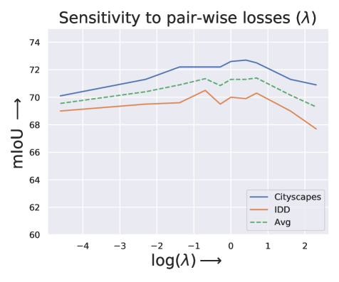
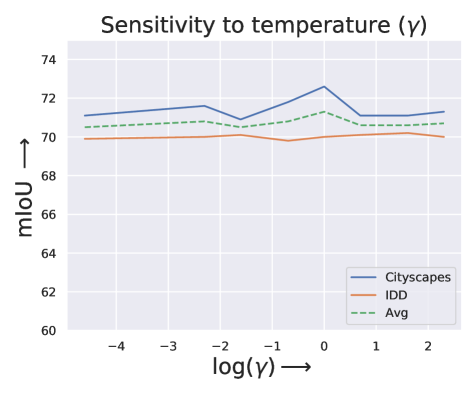
Figure A1: Sensitivity analysis of our proposed CoaST for the 7-class MTDA configuration of GTA5 $\rightarrow$ Cityscapes + IDD. Left: we vary the pair-wise loss weight $\lambda$ and evaluate the mIoU for the target domains. The performance curve remains stable over a wide operating window, and starts to degrade only for extreme values of the $\lambda$. Right: we vary the temperature $\gamma$ and evaluate the mIoU for the target domains. We notice that the average mIoU varies slightly with $\gamma$. On the x-axis we plot the logarithmic values of the hyperparameters for clarity

It can be observed from the Fig. A1 (right) that the performance of CoaST does not vary much while changing the temperature $\gamma$. Indeed, we see that the average mIoU remains in a tight range of 70.5% to 71.3%, even for extreme values of $\gamma$. Note that we vary the value of $\gamma$ between 0.01 and 10 in our ablation study, whereas we report the logarithmic values of $\gamma$ in Fig. A1 on the x-axis for clarity of the plot.

GTA5 $\rightarrow$ Cityscapes + Mapillary
Method	Target	flat	constr	object	nature	sky	human	vehicle	mIoU	Avg.
Individual [35]	C	93.5	80.5	26.0	78.5	78.5	55.1	76.4	69.8	69.7
	M	89.5	72.6	31.0	75.3	94.1	50.7	73.8	69.6
Data Comb. [35]	C	93.1	80.5	24.0	77.9	81.0	52.5	75.0	69.1	68.9
	M	90.0	71.3	31.1	73.0	92.6	46.6	76.6	68.7
Multi-Dis [26]	C	94.5	80.8	22.2	79.2	82.1	47.0	79.0	69.3	69.5
	M	89.4	71.2	29.5	76.2	93.6	50.4	78.3	69.8
MTKT [26]	C	95.0	81.6	23.6	80.1	83.6	53.7	79.8	71.1	70.9
	M	90.6	73.3	31.0	75.3	94.5	52.2	79.8	70.8
ADAS [16]($1024\times 512$)	C	96.4	83.5	35.1	83.6	84.9	62.3	81.3	75.3	73.9
	M	88.6	73.7	41.0	75.4	93.4	58.5	77.2	72.6
CoaST (Ours)	C	94.7	84.4	29.3	81.6	77.7	57.1	81.3	72.3	72.3
	M	89.2	74.9	37.5	74.6	89.2	57.9	82.8	72.3

Table A2: The comparison of CoaST with the state-of-the-art on the 7-classes benchmark using the GTA5 $\rightarrow$ Cityscapes + Mapillary configuration. We observe that CoaST outperforms MTKT on several classes and also on average

Appendix D Quantitative Comparison.

D.1 Detailed Results of the Synthetic to Real Settings

In the Tab. 3 of the main paper, we reported the summary of the performances on all the settings with GTA5 as the source domain. In this section, we report the detailed class-wise results for those settings. The Tab. A2, A3 and A4 detail the results on the 7-class setting while the Tab. A5 detail the results on the 19-class setting. Note that the detailed results of G2CI are already shown in Tab. 1 and the Tab. 2 of the main paper.

In Tab. A2, A3 and A4, we can see that our CoaST outperforms all the baselines and MTKT [26] in 7-class benchmark for most of the classes. These results are in-line with the summarized results reported in the main paper and confirm the consistent gain provided by our CoaST for the majority of the classes. In Tab. A5, we show the detailed comparison with Individual and MTKT in 19-class benchmark. Note that, the detailed comparison with scores reported for every class is not reported in paper introducing CCL [14] and ADAS [16]. Since their codes are not publicly available, we could not provide the detailed class-wise scores. The comparison with CCL [14] and ADAS [16] could only be reported as in Tab. 3 of the main paper.

GTA5 $\rightarrow$ Mapillary + IDD
Method	Target	flat	constr	object	nature	sky	human	vehicle	mIoU	Avg.
Individual [35]	M	89.5	72.6	31.0	75.3	94.1	50.7	73.8	69.6	67.4
	I	91.2	53.1	16.0	78.2	90.7	47.9	78.9	65.1
Data Comb. [35]	M	89.6	71.0	34.2	74.5	92.9	47.3	78.6	69.7	67.9
	I	91.8	54.0	17.4	76.9	92.3	51.4	78.4	66.0
Multi-Dis [26]	M	89.9	71.7	28.7	76.0	93.6	51.6	79.7	70.2	68.1
	I	91.4	54.9	14.6	78.5	93.0	51.1	79.0	66.1
MTKT [26]	M	88.8	73.2	31.5	74.7	94.1	52.5	79.9	70.7	68.3
	I	91.4	55.9	13.5	76.7	92.1	52.3	79.4	65.9
CoaST (Ours)	M	90.5	75.9	37.2	73.6	90.8	57.5	81.3	72.4	70.6
	I	93.3	60.9	19.8	79.3	91.2	54.1	82.6	68.7

Table A3: The comparison of CoaST with the state-of-the-art on the 7-classes benchmark using the GTA5 $\rightarrow$ Mapillary + IDD configuration. We observe that CoaST outperforms MTKT on several classes and also on average

GTA5 $\rightarrow$ Cityscapes + Mapillary + IDD
Method	Target	flat	constr	object	nature	sky	human	vehicle	mIoU	Avg.
Individual [35]	C	93.5	80.5	26.0	78.5	78.5	55.1	76.4	69.8	68.2
	M	89.5	72.6	31.0	75.3	94.1	50.7	73.8	69.6
	I	91.2	53.1	16.0	78.2	90.7	47.9	78.9	65.1
Data Comb. [35]	C	93.6	80.6	26.4	78.1	81.5	51.9	76.4	69.8	67.8
	M	89.2	72.4	32.4	73.0	92.7	41.6	74.9	68.0
	I	92.0	54.6	15.7	77.2	90.5	50.8	78.6	65.6
Multi-Dis [26]	C	94.6	80.0	20.6	79.3	84.1	44.6	78.2	68.8	68.2
	M	89.0	72.5	29.3	75.5	94.7	50.3	78.9	70.0
	I	91.6	54.2	13.1	78.4	93.1	49.6	80.3	65.8
MTKT [26]	C	94.6	80.7	23.8	79.0	84.5	51.0	79.2	70.4	69.1
	M	90.5	73.7	32.5	75.5	94.3	51.2	80.2	71.1
	I	91.7	55.6	14.5	78.0	92.6	49.8	79.4	65.9
ADAS [16]($1024\times 512$)	C	95.8	82.4	38.3	82.4	85.0	60.5	80.2	74.9	71.3
	M	89.2	71.5	45.2	75.8	92.3	56.1	75.4	72.2
	I	89.9	52.7	25.0	78.1	92.1	51.0	77.9	66.7
CoaST (Ours)	C	94.4	80.2	27.0	82.6	88.3	54.6	81.0	72.6	71.7
	M	91.7	74.9	36.2	73.9	92.0	57.5	79.5	72.2
	I	94.6	62.0	21.0	82.6	92.6	55.4	83.7	70.3

Table A4: The comparison of CoaST with the state-of-the-art on the 7-classes benchmark using the GTA5 $\rightarrow$ Cityscapes + Mapillary + IDD configuration. We observe that CoaST outperforms MTKT on several classes and also on average. Particularly, the gain in performance for CoaST over MTKT for the IDD is fairly substantial

GTA5 $\rightarrow$ Cityscapes + IDD
Method	Target	road	sidewalk	building	walk	fence	pole	light	sign	veg	terrain	sky	person	rider	car	truck	bus	train	motor	bike	mIoU	Avg.
Individual [35]	C	88.8	23.8	81.5	27.7	27.3	31.7	33.2	22.9	83.1	27.0	76.4	58.5	28.9	84.3	30.0	36.8	0.3	27.7	33.1	43.3	43.5
	I	94.1	24.4	66.1	31.3	22.0	25.4	9.3	26.7	80.0	31.4	93.5	48.7	43.8	71.4	49.4	28.5	0	48.7	34.3	43.6
MTKT	C	88.5	37.2	79.1	22.8	19.8	26.3	33.8	16.7	84.8	34.2	80.5	54.9	15.0	84.1	27.5	41.2	0.3	27.9	7.0	41.7	42.5
	I	82.7	24.2	54.2	29.3	22.0	24.8	8.4	52.0	78.7	18.2	92.1	38.6	51.0	72.5	60.8	27.6	0	54.5	14.1	43.3
CoaST (Ours)	C	81.7	38.3	71.0	33.3	30.7	35.1	38.2	37.6	86.4	46.9	81.9	63.4	27.4	84.5	29.4	45.6	0.3	32.6	31.3	47.1	48.2
	I	85.7	36.1	65.1	33.2	23.7	32.8	19.0	62.9	82.5	29.5	91.8	52.1	55.3	83.4	62.9	46.1	0	55.5	18.5	49.3
GTA5 $\rightarrow$ Cityscapes + Mapillary
Method	Target	road	sidewalk	building	walk	fence	pole	light	sign	veg	terrain	sky	person	rider	car	truck	bus	train	motor	bike	mIoU	Avg.
Individual [35]	C	88.8	23.8	81.5	27.7	27.3	31.7	33.2	22.9	83.1	27.0	76.4	58.5	28.9	84.3	30.0	36.8	0.3	27.7	33.1	43.3	44.7
	M	81.1	18.6	74.8	23.9	28.9	30.3	35.7	33.7	78.4	40.7	93.3	49.5	42.3	80.4	35.1	34.2	17.8	41.8	36.1	46.1
MTKT [26]	C	89.2	36.1	81.5	31.6	22.1	28.4	31.4	13.8	85.1	34.3	83.5	57.6	19.1	86.1	36.0	44.1	0.4	32.5	6.1	43.1	45.4
	M	86.8	38.7	78.7	27.0	28.4	29.5	37.3	34.6	78.4	42.3	94.9	53.7	37.9	84.2	41.1	34.5	15.5	44.0	18.0	47.6
CoaST (Ours)	C	82.1	36.2	77.5	47.4	34.9	36.7	42.0	36.6	87.2	38.6	80.8	60.6	21.6	86.1	33.3	45.7	2.5	26.2	34.7	47.9	49.9
	M	84.7	44.4	80.3	35.7	27.7	37.2	45.1	51.8	73.8	42.4	93.7	64.5	42.2	83.9	49.0	44.0	10.0	38.5	35.6	51.8
GTA5 $\rightarrow$ Mapillary + IDD
Method	Target	road	sidewalk	building	walk	fence	pole	light	sign	veg	terrain	sky	person	rider	car	truck	bus	train	motor	bike	mIoU	Avg.
Individual [35]	M	81.1	18.6	74.8	23.9	28.9	30.3	35.7	33.7	78.4	40.7	93.3	49.5	42.3	80.4	35.1	34.2	17.8	41.8	36.1	46.1	44.9
	I	94.1	24.4	66.1	31.3	22.0	25.4	9.3	26.7	80.0	31.4	93.5	48.7	43.8	71.4	49.4	28.5	0	48.7	34.3	43.6
MTKT [26]	M	85.4	42.8	78.6	28.9	32.8	31.0	32.8	35.4	79.8	45.0	95.1	54.1	34.3	82.5	36.2	34.1	9.5	40.6	37.6	48.2	45.4
	I	82.1	14.1	56.4	31.4	21.3	28.6	12.5	43.0	81.0	26.9	93.6	35.8	46.9	76.2	56.9	39.5	0	50.5	13.4	42.6
CoaST (Ours)	M	79.4	35.3	81.0	34.6	30.9	37.8	43.7	52.7	74.1	45.0	93.4	63.7	43.2	84.9	48.2	51.3	5.3	39.8	36.6	51.6	50.6
	I	87.1	30.1	66.3	34.7	21.8	34.5	18.9	66.0	80.6	41.7	91.3	52.8	55.8	83.7	58.4	48.0	0	55.6	13.2	49.5
GTA5 $\rightarrow$ Cityscapes + Mapillary + IDD
Method	Target	road	sidewalk	building	walk	fence	pole	light	sign	veg	terrain	sky	person	rider	car	truck	bus	train	motor	bike	mIoU	Avg.
Individual [35]	C	88.8	23.8	81.5	27.7	27.3	31.7	33.2	22.9	83.1	27.0	76.4	58.5	28.9	84.3	30.0	36.8	0.3	27.7	33.1	43.3	43.3
	M	81.1	18.6	74.8	23.9	28.9	30.3	35.7	33.7	78.4	40.7	93.3	49.5	42.3	80.4	35.1	34.2	17.8	41.8	36.1	46.1
	I	94.1	24.4	66.1	31.3	22.0	25.4	9.3	26.7	80.0	31.4	93.5	48.7	43.8	71.4	49.4	28.5	0	48.7	34.3	43.6
MTKT [26]	C	85.9	33.7	81.2	30.2	20.0	31.3	32.7	17.5	84.1	33.2	80.8	56.1	16.8	83.2	26.0	39.2	10.9	24.4	13.7	42.2	43.9
	M	85.9	42.1	76.1	29.1	28.7	30.3	35.1	34.4	76.6	43.1	93.7	55.2	31.1	82.7	37.8	31.8	20.8	37.8	17.3	46.8
	I	83.1	16.9	55.7	34.7	21.3	27.6	8.0	48.6	77.7	26.9	91.9	36.7	46.2	74.2	56.1	41.3	0	48.7	15.7	42.7
CoaST (Ours)	C	88.4	43.0	80.0	30.9	29.4	37.6	36.9	42.1	86.2	40.9	81.5	60.1	15.4	85.5	33.5	44.5	4.6	30.7	26.7	47.2	49.1
	M	82.8	44.8	79.5	32.3	37.9	38.3	38.2	52.4	76.0	45.5	92.9	65.2	39.2	85.8	51.0	43.1	6.2	38.2	27.3	51.4
	I	86.9	29.0	64.1	31.2	20.2	36.7	14.8	51.9	82.3	48.2	92.7	51.8	53.6	83.8	60.7	46.6	0	50.5	20.6	48.7

Table A5: The detailed class-wise comparison of CoaST in the 19-class setting with the existing state-of-the-art methods. In all the experiments, GTA5 is considered as the source domain and the various combinations of the other benchmarks are considered as the target domains. In all the configurations our CoaST clearly outperforms the existing baselines by a clear margin

D.2 Synthetic to Real scenario: summary of all the Settings.

In the main paper, we report in Tab. 3 the average mIoU considering all the possible target configurations on the 19-classes Benchmark in the Synthetic to Real scenario. We now report the results on the 7-classes Benchmark in Tab. A6. In short, we observe that CoaST obtains performance on par with ADAS [16]. CoaST obtains the pest average performance in three configurations over four. These experiments demonstrate again the robustness of our approach.

7-classes Benchmark
Target			method	mIoU			mIoU
C	I	M		C	I	M	Avg.
$\surd$	$\surd$	-	MTKT [26]	70.4	65.9	-	68.2
			ADAS [16]($1024\times 512$)	75.4	66.9	-	71.2
			CoaST (Ours)	72.6	70.0	-	71.3
$\surd$	-	$\surd$	MTKT [26]	71.1	-	70.8	71.0
			ADAS [16]($1024\times 512$)	75.3	-	72.6	73.9
			CoaST (Ours)	72.3	-	72.3	72.3
-	$\surd$	$\surd$	MTKT [26]	-	65.9	70.7	68.3
			ADAS [16]($1024\times 512$)	-	-	-	-
			CoaST (Ours)	-	68.7	72.4	70.6
$\surd$	$\surd$	$\surd$	MTKT [26]	70.4	65.9	71.1	69.1
			ADAS [16]($1024\times 512$)	74.9	66.7	72.2	71.3
			CoaST (Ours)	72.6	70.3	72.2	71.7

Table A6: Summary of performances obtained on the 7-classes Benchmark with different dataset configurations. Cityscapes, IDD and Mapillary are referred to as C, I and M respectively. We report the mIoU averaged over the target domains.

D.3 Detailed Results of the Real to Real Settings

Here we show the comparison with MTKT in all the Real to Real settings on the 7-class benchmark. We observe from the Tab. A7 that CoaST can clearly outperform MTKT in all the real to real configurations. This again proves the versatility of CoaST as it can yield better performance when trained on both synthetic and real source domains.

Cityscapes $\rightarrow$ Mapillary + IDD
Method	Target	flat	constr	object	nature	sky	human	vehicle	mIoU	Avg.
MTKT[26]	M	88.3	70.4	31.6	75.9	94.4	50.9	77.0	69.8	69.0
	I	93.6	54.9	18.6	84.0	94.5	53.4	79.2	68.3
CoaST (Ours)	M	90.2	73.4	37.2	78.8	92.3	59.2	84.1	73.6	72.6
	I	95.1	58.0	26.6	85.4	93.0	59.0	83.9	71.6
Mapillary $\rightarrow$ Cityscapes + IDD
Method	Target	flat	constr	object	nature	sky	human	vehicle	mIoU	Avg.
MTKT[26]	C	94.7	81.9	35.6	83.0	84.7	57.0	83.9	74.4	72.7
	I	95.2	61.6	24.6	85.4	94.3	55.7	81.1	71.1
CoaST (Ours)	C	95.6	84.4	36.7	83.9	88.2	58.2	85.8	76.1	74.8
	I	95.5	64.6	31.1	85.8	94.6	58.2	84.7	73.5
IDD $\rightarrow$ Cityscapes + Mapillary
Method	Target	flat	constr	object	nature	sky	human	vehicle	mIoU	Avg.
MTKT[26]	C	96.7	82.8	31.0	84.7	89.8	60.2	85.1	75.8	73.9
	M	90.4	71.2	33.8	79.1	95.8	55.3	79.0	72.1
CoaST (Ours)	C	96.5	84.3	33.6	84.7	89.1	58.3	85.8	76.0	75.7
	M	91.0	76.3	39.7	82.2	96.0	59.0	83.1	75.3

Table A7: The detailed comparison of CoaST with the state-of-the-art on the 7-classes benchmark in all Real to Real scenarios. CoaST clearly outperforms MTKT in all the real to real configuration.

D.4 Comparison with other MTDA methods.

In this section, we compare our methods with other MTDA methods in the literature that have been proposed for object recognition. Following CCL [14], we report the numbers of CoaST on the 19-class benchmark in the Tab. A8. Note that only CCL [14] and CoaST are specifically designed for semantic segmentation. The baselines in the MTDA setting [11, 22] that are designed for object recognition perform sub-optimally with respect CCL [14]. However, CoaST surpasses CCL [14] by a non-trivial margin, validating the importance of data driven image stylization for the MTDA in semantic segmentation.

GTA5 $\rightarrow$ Cityscapes + IDD
Setting	Method	mIoU		Avg.
		C	I
DG	Yue et al. [40]	42.1	42.8	42.5
MTDA	MTDA-ITA [11]	40.3	41.2	40.8
	MT-MTDA [22]	43.2	44.0	43.6
	CCL [14]	45.0	46.0	45.5
	CoaST (Ours)	47.1	49.3	48.2

Table A8: The quantitative comparison of our CoaST with different MTDA methods on the 19-class benchmark for the GTA5 $\rightarrow$ Cityscapes + IDD configuration. CoaST outperforms the considered MTDA baselines that are designed for either object recognition or semantic segmentation. DG stands for domain generalization setting and a method designed for such a setting is also under performed by CoaST

D.5 Direct Transfer to Unseen Domains

Similar to [26], we directly test our adapted model on a new (or unseen) target domain to evaluate the generalization ability of our model. This setting is often referred to as open-compound domain adaptation in the literature. In the Tab. A9, we report the comparison of the generalization ability with other methods on 7-class benchmark. We can observe that among considered MTDA baselines, our CoaST has the best generalization ability. This hints at the fact that our proposed cooperative self-training realized with feature stylization can induce better generalizability.

Direct Transfer to an Unseen Target Domain
Setup	Method	Test	flat	constr	object	nature	sky	human	vehicle	mIoU
G $\rightarrow$ C + I	Data Comb. [35]	M	88.4	71.0	31.0	72.4	92.0	37.4	74.7	66.7
	Multi-Dis[26]		89.2	72.1	21.7	73.8	94.0	34.8	75.9	65.9
	MTKT[26]		89.8	74.0	30.4	74.1	93.6	52.6	79.4	70.6
	CoaST (Ours)		91.6	73.9	34.8	77.8	93.0	57.7	81.9	72.9
G $\rightarrow$ C + M	Data Comb.[35]	I	91.6	54.7	13.9	76.5	90.9	48.3	77.5	64.8
	Multi-Dis[26]		91.2	54.6	12.9	77.7	92.5	50.3	78.6	65.4
	MTKT[26]		91.5	56.1	12.3	76.1	90.9	51.4	79.2	65.4
	CoaST (Ours)		93.2	59.7	17.1	80.1	91.0	51.7	81.2	67.7

Table A9: The quantitative comparison for direct transfer to new (or unseen) domains in 7-class benchmark. GTA5, Cityscapes, Mapillary and IDD are referred to as G, C, M and I, respectively. The Test column denotes the unseen target domain where the models have been evaluated

References

- [1] Vijay Badrinarayanan, Alex Kendall, and Roberto Cipolla. Segnet: A deep convolutional encoder-decoder architecture for image segmentation. IEEE Transactions on Pattern Analysis and Machine Intelligence (TPAMI), 39(12):2481–2495, 2017.
- [2] Wei-Lun Chang, Hui-Po Wang, Wen-Hsiao Peng, and Wei-Chen Chiu. All about structure: Adapting structural information across domains for boosting semantic segmentation. In Proceedings of the IEEE Conference on Computer Vision and Pattern Recognition (CVPR), pages 1900–1909, 2019.
- [3] Liang-Chieh Chen, George Papandreou, Iasonas Kokkinos, Kevin Murphy, and Alan L Yuille. Deeplab: Semantic image segmentation with deep convolutional nets, atrous convolution, and fully connected crfs. IEEE Transactions on Pattern Analysis and Machine Intelligence (TPAMI), 40(4):834–848, 2017.
- [4] Liang-Chieh Chen, George Papandreou, Florian Schroff, and Hartwig Adam. Rethinking atrous convolution for semantic image segmentation. arXiv preprint arXiv:1706.05587, 2017.
- [5] Yun-Chun Chen, Yen-Yu Lin, Ming-Hsuan Yang, and Jia-Bin Huang. Crdoco: Pixel-level domain transfer with cross-domain consistency. In Proceedings of the IEEE Conference on Computer Vision and Pattern Recognition (CVPR), pages 1791–1800, 2019.
- [6] Ziliang Chen, Jingyu Zhuang, Xiaodan Liang, and Liang Lin. Blending-target domain adaptation by adversarial meta-adaptation networks. In Proceedings of the IEEE Conference on Computer Vision and Pattern Recognition (CVPR), pages 2248–2257, 2019.
- [7] Marius Cordts, Mohamed Omran, Sebastian Ramos, Timo Rehfeld, Markus Enzweiler, Rodrigo Benenson, Uwe Franke, Stefan Roth, and Bernt Schiele. The cityscapes dataset for semantic urban scene understanding. In Proceedings of the IEEE Conference on Computer Vision and Pattern Recognition (CVPR), pages 3213–3223, 2016.
- [8] Gabriela Csurka, Riccardo Volpi, and Boris Chidlovskii. Unsupervised domain adaptation for semantic image segmentation: a comprehensive survey. arXiv preprint arXiv:2112.03241, 2021.
- [9] Yarin Gal and Zoubin Ghahramani. Dropout as a bayesian approximation: Representing model uncertainty in deep learning. In International Conference on Machine Learning (ICML), pages 1050–1059, 2016.
- [10] Yaroslav Ganin and Victor Lempitsky. Unsupervised domain adaptation by backpropagation. In International Conference on Machine Learning (ICML), pages 1180–1189, 2015.
- [11] Behnam Gholami, Pritish Sahu, Ognjen Rudovic, Konstantinos Bousmalis, and Vladimir Pavlovic. Unsupervised multi-target domain adaptation: An information theoretic approach. IEEE Transactions on Image Processing (TIP), 29:3993–4002, 2020.
- [12] Geoffrey Hinton, Oriol Vinyals, Jeff Dean, et al. Distilling the knowledge in a neural network. In Workshop at Advances in Neural Information Processing Systems (NIPS), 2014.
- [13] Judy Hoffman, Eric Tzeng, Taesung Park, Jun-Yan Zhu, Phillip Isola, Kate Saenko, Alexei Efros, and Trevor Darrell. Cycada: Cycle-consistent adversarial domain adaptation. In International Conference on Machine Learning (ICML), pages 1989–1998, 2018.
- [14] Takashi Isobe, Xu Jia, Shuaijun Chen, Jianzhong He, Yongjie Shi, Jianzhuang Liu, Huchuan Lu, and Shengjin Wang. Multi-target domain adaptation with collaborative consistency learning. In Proceedings of the IEEE Conference on Computer Vision and Pattern Recognition (CVPR), pages 8187–8196, 2021.
- [15] Myeongjin Kim and Hyeran Byun. Learning texture invariant representation for domain adaptation of semantic segmentation. In Proceedings of the IEEE Conference on Computer Vision and Pattern Recognition (CVPR), pages 12975–12984, 2020.
- [16] Seunghun Lee, Wonhyeok Choi, Changjae Kim, Minwoo Choi, and Sunghoon Im. Adas: A direct adaptation strategy for multi-target domain adaptive semantic segmentation. In Proceedings of the IEEE/CVF Conference on Computer Vision and Pattern Recognition (CVPR), pages 19196–19206, 2022.
- [17] Guangrui Li, Guoliang Kang, Wu Liu, Yunchao Wei, and Yi Yang. Content-consistent matching for domain adaptive semantic segmentation. In Proceedings of the IEEE European Conference on Computer Vision (ECCV), pages 440–456, 2020.
- [18] Peilun Li, Xiaodan Liang, Daoyuan Jia, and Eric P Xing. Semantic-aware grad-gan for virtual-to-real urban scene adaption. In British Machine Vision Conference (BMVC), page 73, 2018.
- [19] Yunsheng Li, Lu Yuan, and Nuno Vasconcelos. Bidirectional learning for domain adaptation of semantic segmentation. In Proceedings of the IEEE Conference on Computer Vision and Pattern Recognition (CVPR), pages 6936–6945, 2019.
- [20] Zak Murez, Soheil Kolouri, David Kriegman, Ravi Ramamoorthi, and Kyungnam Kim. Image to image translation for domain adaptation. In Proceedings of the IEEE Conference on Computer Vision and Pattern Recognition (CVPR), pages 4500–4509, 2018.
- [21] Gerhard Neuhold, Tobias Ollmann, Samuel Rota Bulo, and Peter Kontschieder. The mapillary vistas dataset for semantic understanding of street scenes. In Proceedings of the IEEE International Conference on Computer Vision (ICCV), pages 4990–4999, 2017.
- [22] Le Thanh Nguyen-Meidine, Atif Belal, Madhu Kiran, Jose Dolz, Louis-Antoine Blais-Morin, and Eric Granger. Unsupervised multi-target domain adaptation through knowledge distillation. In Proceedings of the IEEE/CVF Winter Conference on Applications of Computer Vision (WACV), pages 1339–1347, 2021.
- [23] Xingchao Peng, Zijun Huang, Ximeng Sun, and Kate Saenko. Domain agnostic learning with disentangled representations. In International Conference on Machine Learning (ICML), pages 5102–5112, 2019.
- [24] Stephan R Richter, Vibhav Vineet, Stefan Roth, and Vladlen Koltun. Playing for data: Ground truth from computer games. In Proceedings of the IEEE European Conference on Computer Vision (ECCV), pages 102–118, 2016.
- [25] Subhankar Roy, Evgeny Krivosheev, Zhun Zhong, Nicu Sebe, and Elisa Ricci. Curriculum graph co-teaching for multi-target domain adaptation. In Proceedings of the IEEE Conference on Computer Vision and Pattern Recognition (CVPR), pages 5351–5360, 2021.
- [26] Antoine Saporta, Tuan-Hung Vu, Matthieu Cord, and Patrick Pérez. Multi-target adversarial frameworks for domain adaptation in semantic segmentation. In Proceedings of the IEEE International Conference on Computer Vision (ICCV), pages 9072–9081, 2021.
- [27] Tong Shen, Dong Gong, Wei Zhang, Chunhua Shen, and Tao Mei. Regularizing proxies with multi-adversarial training for unsupervised domain-adaptive semantic segmentation. arXiv preprint arXiv:1907.12282, 2019.
- [28] Kihyuk Sohn, David Berthelot, Nicholas Carlini, Zizhao Zhang, Han Zhang, Colin A Raffel, Ekin Dogus Cubuk, Alexey Kurakin, and Chun-Liang Li. Fixmatch: Simplifying semi-supervised learning with consistency and confidence. Advances in Neural Information Processing Systems (NIPS), 33:596–608, 2020.
- [29] Zhiqiang Tang, Yunhe Gao, Yi Zhu, Zhi Zhang, Mu Li, and Dimitris N Metaxas. Crossnorm and selfnorm for generalization under distribution shifts. In Proceedings of the IEEE International Conference on Computer Vision (ICCV), pages 52–61, 2021.
- [30] Marco Toldo, Umberto Michieli, Gianluca Agresti, and Pietro Zanuttigh. Unsupervised domain adaptation for mobile semantic segmentation based on cycle consistency and feature alignment. Image and Vision Computing (Image Vis Comput), 95:103889, 2020.
- [31] Antonio Torralba and Alexei A Efros. Unbiased look at dataset bias. In Proceedings of the IEEE Conference on Computer Vision and Pattern Recognition (CVPR), pages 1521–1528, 2011.
- [32] Yi-Hsuan Tsai, Wei-Chih Hung, Samuel Schulter, Kihyuk Sohn, Ming-Hsuan Yang, and Manmohan Chandraker. Learning to adapt structured output space for semantic segmentation. In Proceedings of the IEEE Conference on Computer Vision and Pattern Recognition (CVPR), pages 7472–7481, 2018.
- [33] Dmitry Ulyanov, Andrea Vedaldi, and Victor Lempitsky. Instance normalization: The missing ingredient for fast stylization. arXiv preprint arXiv:1607.08022, 2016.
- [34] Girish Varma, Anbumani Subramanian, Anoop Namboodiri, Manmohan Chandraker, and CV Jawahar. Idd: A dataset for exploring problems of autonomous navigation in unconstrained environments. In 2019 IEEE Winter Conference on Applications of Computer Vision (WACV), pages 1743–1751, 2019.
- [35] Tuan-Hung Vu, Himalaya Jain, Maxime Bucher, Mathieu Cord, and Patrick Pérez. Advent: Adversarial entropy minimization for domain adaptation in semantic segmentation. In Proceedings of the IEEE Conference on Computer Vision and Pattern Recognition (CVPR), pages 2517–2526, 2019.
- [36] Zhonghao Wang, Mo Yu, Yunchao Wei, Rogerio Feris, Jinjun Xiong, Wen-mei Hwu, Thomas S Huang, and Honghui Shi. Differential treatment for stuff and things: A simple unsupervised domain adaptation method for semantic segmentation. In Proceedings of the IEEE Conference on Computer Vision and Pattern Recognition (CVPR), pages 12635–12644, 2020.
- [37] Zuxuan Wu, Xintong Han, Yen-Liang Lin, Mustafa Gokhan Uzunbas, Tom Goldstein, Ser Nam Lim, and Larry S Davis. Dcan: Dual channel-wise alignment networks for unsupervised scene adaptation. In Proceedings of the IEEE European Conference on Computer Vision (ECCV), pages 518–534, 2018.
- [38] Xu Yang, Cheng Deng, Tongliang Liu, and Dacheng Tao. Heterogeneous graph attention network for unsupervised multiple-target domain adaptation. IEEE Transactions on Pattern Analysis and Machine Intelligence (TPAMI), 2020.
- [39] Yanchao Yang and Stefano Soatto. Fda: Fourier domain adaptation for semantic segmentation. In Proceedings of the IEEE Conference on Computer Vision and Pattern Recognition (CVPR), pages 4085–4095, 2020.
- [40] Xiangyu Yue, Yang Zhang, Sicheng Zhao, Alberto Sangiovanni-Vincentelli, Kurt Keutzer, and Boqing Gong. Domain randomization and pyramid consistency: Simulation-to-real generalization without accessing target domain data. In Proceedings of the IEEE/CVF International Conference on Computer Vision (ICCV), pages 2100–2110, 2019.
- [41] Pan Zhang, Bo Zhang, Ting Zhang, Dong Chen, Yong Wang, and Fang Wen. Prototypical pseudo label denoising and target structure learning for domain adaptive semantic segmentation. In Proceedings of the IEEE Conference on Computer Vision and Pattern Recognition (CVPR), pages 12414–12424, 2021.
- [42] Qiming Zhang, Jing Zhang, Wei Liu, and Dacheng Tao. Category anchor-guided unsupervised domain adaptation for semantic segmentation. Advances in Neural Information Processing Systems (NIPS), 32, 2019.
- [43] Zhedong Zheng and Yi Yang. Unsupervised scene adaptation with memory regularization in vivo. In AAAI International Joint Conference on Artificial Intelligence (IJCAI), pages 1076–1082, 2020.
- [44] Zhedong Zheng and Yi Yang. Rectifying pseudo label learning via uncertainty estimation for domain adaptive semantic segmentation. International Journal of Computer Vision (IJCV), 2021. doi:10.1007/s11263-020-01395-y.
- [45] Bolei Zhou, Hang Zhao, Xavier Puig, Sanja Fidler, Adela Barriuso, and Antonio Torralba. Scene parsing through ade20k dataset. In Proceedings of the IEEE Conference on Computer Vision and Pattern Recognition (CVPR), pages 633–641, 2017.
- [46] Kaiyang Zhou, Yongxin Yang, Yu Qiao, and Tao Xiang. Domain generalization with mixstyle. In Proceedings of the International Conference on Learning Representations (ICLR), 2021.
- [47] Xinge Zhu, Hui Zhou, Ceyuan Yang, Jianping Shi, and Dahua Lin. Penalizing top performers: Conservative loss for semantic segmentation adaptation. In Proceedings of the IEEE European Conference on Computer Vision (ECCV), pages 568–583, 2018.
- [48] Yang Zou, Zhiding Yu, BVK Kumar, and Jinsong Wang. Unsupervised domain adaptation for semantic segmentation via class-balanced self-training. In Proceedings of the IEEE European Conference on Computer Vision (ECCV), pages 289–305, 2018.