Charged anisotropic white dwarfs in $f(R,T)$ gravity

Abstract

In the context of $f(R,T)=R+2\beta T$ gravity, where $R$ is the Ricci scalar and $T$ is the trace of the energy-momentum tensor, the equilibrium structure of charged anisotropic white dwarfs (WDs) is studied. The stellar equations for the general case are derived and numerical solutions are found for the Chandrasekhar equation of state (EoS) and a charge density distribution proportional to the energy density $\rho_{ch}=\alpha\rho$. By adjusting different parameters, the properties of the solutions under various conditions are compared. Most importantly, by going beyond the trivial WD in GR in various ways, the solutions may exhibit super-Chandrasekhar behavior. This paper is a study of a WD structure, and the results obtained may have a contrasting effect on astronomical observations such as superluminous type Ia supernovae.

I Introduction

General relativity(GR) has withstood almost all observations and experimental tests from weak gravity (e.g., Mercury’s perihelion shift, gravitational lensing, gravitational redshift, etc. at the scale of the solar system) and strong gravity (e.g. pulsar binary systems), and is therefore a beautiful and successful theory of gravity. With the discovery of Type Ia supernovae [1], the cosmic microwave background radiation (CWBR) [2, 3], and most importantly, the accelerating expansion of the universe, Einstein’s theory have shown increasing limitations. Even in a purely academic interest, there is a desire to explore theories outside the standard GR framework [4]. Hence many alternative models have been proposed [5].

The simplest correction scheme is to replace the Einstein-Hilbert action with a general function of the Ricci scalar $R$ to obtain $f(R)$ gravitation[6, 7], where $R$ is treated as a redundant degree of freedom. As a famous example, the Starobinsky theory[8] is used to deal with many questions about stars. $f(R)=R^{1+\varepsilon}$ gravity is applied as a correction close to GR in the study of compact astronomical objects[9].

Further, coupling in the trace $T=g_{ab}T^{ab}$ of the matter energy tensor gives the $f(R,T)$ theory[10], which further explores the role of matter in the gravitational field. The $f(R,T)$ theory has special significance for the static equilibrium structure of compact stars, see [11, 12, 13, 14, 15, 16, 17, 18, 19]. This has been an active research area in the last few years, and in the present work, we adopt a similar path.

White dwarfs (WD), quark stars (QS), neutron stars (NS), etc. are the compact astronomical objects of interest. A white dwarf is a stellar core remnant composed mostly of electron-degenerate matter. White dwarfs are thought to be the final evolutionary state of stars whose mass is not high enough to become a neutron star or black hole. This includes over $97\%$ of the other stars in the Milky Way. Chandrasekhar has long established a mass limit for WD[20] that its mass cannot exceed $1.44M_{\odot}$. Type Ia supernova (SNIa) explosions may occur when WD masses exceed this limit, with equal brightness considered standard candles. However, the discovery of a group of super-bright supernovae[21, 22] has driven the hypothesis that their ancestors were WDs with super-Chandrasekhar masses. In the scope of GR and modified gravity (MG), various possible WD structures with Chandrasekhar equation of state (EoS)[23] have been extensively studied, including uniformly charged WD under GR [24], WD under $f(R,T)$ gravity[11], charged WD under GR [25], charged WD under $f(R,T)$ gravity [12], the charge of the latter two are mainly concentrated on the surface of stars.

The idea of stellar structure discussed in this paper mainly comes from the studies of several authors for QS. A quark star is a hypothetical type of compact, exotic star, where extremely high core temperature and pressure have forced nuclear particles to form quark matter, a continuous state of matter consisting of free quarks. For QS, more abundant structures were considered[26, 13, 14, 15, 16, 17, 18, 19], including: surface or internal charge, isotropic or anisotropic pressure, GR or $f(R,T)$ gravity. Usually, when dealing with QS, the MIT Bag Model EoS is chosen, although some authors [19] are happy to use EoS with $\mathcal{O}(m_{\text{s}}^{4})$ correction term to obtain a more accurate case. Although the structure of WD is solved in this paper, a charge density proportional to the energy density and anisotropic pressure distribution are introduced.

This paper is organized as follows. Following this introduction(I), in Sec. II, we briefly review $f(R,T)$ gravity and derive the field equations in the presence of matter and electromagnetic fields. In Sec. III, the modified Tolman-Oppenheimer-Volkoff (TOV) equation(Sec. III.1) is obtained by considering the spherical symmetry metric. The selected Chandrasekhar EoS(Sec. III.2) and charge distribution(Sec. III.3) are also presented in two subsections in Sec. III. In the Sec. IV, the numerical solution of the equation is obtained. The results are briefly analyzed. Finally, in Sec. V, conclusions are drawn from the results.

II $f(R,T)$ gravity formalism

Proposed by Harko et al.[10], $f(R,T)$ gravity is a generalization based on $f(R)$ [7, 6]. where the action of the gravitational field contains an arbitrary function with respect to the Ricci scalar $R$ and the trace $T$ of the energy-momentum tensor. When there is a matter field and a gravitational field, consider the following actions

$$S= \int\mathrm{d}^{4}x\sqrt{-g}\left[\mathcal{L}_{g}+\mathcal{L}_{m}+\mathcal{L}_{e}\right]$$ (1)

$$= \int\mathrm{d}^{4}x\sqrt{-g}\left[\frac{1}{16\pi}f(R,T)+\mathcal{L}_{m}+\mathcal{L}_{e}\right],$$

where $g$ is the determinant of the space-time metric $g_{ab}$ and $\mathcal{L}_{m}$ is the Lagrangian density of the matter field. $\mathcal{L}_{e}$ is the Lagrangian density of the electromagnetic field with the following form

$$\mathcal{L}_{e}=j^{a}A_{a}-\frac{1}{16\pi}F_{ab}F^{ab},$$ (2)

where $j^{a}=\rho_{\text{ch}}u^{a}$ is the four-current density with $\rho_{\text{ch}}$ being the electric charge density and $u^{a}$ being the four-velocity, respectively. $A_{a}$ is the electromagnetic four-potential, and $F_{ab}=\nabla_{a}A_{b}-\nabla_{b}A_{a}$ is the electromagnetic field strength tensor naturally. Additionally, $\nabla_{a}$ is a covariant derivative operator adapted to the metric $g_{ab}$.

The field equation can be obtained by the variation of action respect to metric. Firstly, the action of electromagnetic field and matter are varied to obtain the electromagnetic energy-momentum tensor and the matter energy-momentum tensor, respectively

$$\mathcal{E}_{ab}=\frac{-2}{\sqrt{-g}}\frac{\delta S_{e}}{\delta g^{ab}}=\frac{1}{4\pi}\left[g^{cd}F_{ac}F_{bd}-\frac{1}{4}g_{ab}F_{cd}F^{cd}\right],$$ (3)

$$\mathcal{M}_{ab}=\frac{-2}{\sqrt{-g}}\frac{\delta S_{m}}{\delta g^{ab}}=g_{ab}\mathcal{L}_{m}-2\frac{\partial\mathcal{L}_{m}}{\partial g^{ab}}.$$ (4)

The total energy-momentum tensor is the sum of the two, namely $T_{ab}=\mathcal{M}_{ab}+\mathcal{E}_{ab}$. Considering that the electromagnetic energy-momentum tensor is traceless, further $T\equiv g^{ab}T_{ab}=g^{ab}\mathcal{M}_{ab}\equiv\mathcal{M}$.

The variation of the action of the gravitational field is continued with a view to obtaining the equations of the gravitational field.

$$\frac{16\pi}{\sqrt{-g}}\frac{\delta S_{g}}{\delta g^{ab}}=f_{R}R_{ab}-\frac{1}{2}g_{ab}f +\left(g_{ab}\square-\nabla_{a}\nabla_{b}\right)f_{R}$$ (5)

$$+f_{T}\left(\mathcal{M}_{ab}+\Theta_{ab}\right),$$

where $f_{R}\equiv\partial f(R,T)/\partial R$, $f_{T}\equiv\partial f(R,T)/\partial T$, $\square=\nabla^{a}\nabla_{a}$ is the d’Alembert operator, and

$$\Theta_{ab}\equiv g^{cd}\frac{\delta\mathcal{M}_{cd}}{\delta g^{ab}}=-2\mathcal{M}_{ab}+g_{ab}\mathcal{L}_{m}-2g^{cd}\frac{\partial^{2}\mathcal{L}_{m}}{\partial g^{ab}\partial g^{cd}}.$$ (6)

According to the variational principle $\delta S=0$, we can get the equation of motion of the gravitational field

$$f_{R}R_{ab}-\frac{1}{2}g_{ab} f+\left(g_{ab}\square-\nabla_{a}\nabla_{b}\right)f_{R}$$ (7)

$$=8\pi\left(\mathcal{M}_{ab}+\mathcal{E}_{ab}\right)-f_{T}\left(\mathcal{M}_{ab}+\Theta_{ab}\right).$$

As in the case of $f(R)$ theory, the Ricci scalar is treated as a redundant degree of freedom whose equation of motion can be obtained by taking the trace of the tensor equation of motion

$$3\square f_{R}+Rf_{R}-2f=8\pi\mathcal{M}-f_{T}\left(\mathcal{M}+\Theta\right).$$ (8)

Similar to the case in GR, taking the covariant derivative of the tensor equation of motion eq.7 yields an equation for the energy-momentum tensor

$$\nabla^{a}\mathcal{M}_{ab}=\frac{f_{T}}{8\pi-f_{T}} [\left(\mathcal{M}_{ab}+\Theta_{ab}\right)\nabla^{a}\ln f_{T}+\nabla^{a}\Theta_{ab}$$ (9)

$$-\frac{1}{2}g_{ab}\nabla^{a}T-\frac{8\pi}{f_{T}}\nabla^{a}\mathcal{E}_{ab}].$$

It can be verified that if $f(R,T)=R$ is taken, the theory will return to the standard case of GR: eq.7 will return to Einstein’s gravitational field equation, while eq.9 will return to energy-momentum conservation.

Next, I will take $f(R,T)=R+2\beta T$, following the examples in [11, 13, 14, 12, 15, 16, 17, 18, 27, 28, 29, 19].

III stellar structure equations

III.1 modified TOV equations

In order to further expand the equation into a component form, a static spherically symmetric space-time line element is chosen

$$\mathrm{d}s^{2}=-\mathrm{e}^{2\psi(r)}\mathrm{d}t^{2}+\mathrm{e}^{2\lambda(r)}\mathrm{d}r^{2}+r^{2}\left(\mathrm{d}\theta^{2}+\sin^{2}\theta\mathrm{d}\phi^{2}\right).$$ (10)

At this point, the Maxwell equation obeyed by the electromagnetic field can be written more explicitly

$$\nabla^{a}F_{ab}=-4\pi j_{b},\nabla_{[a}F_{bc]}=0.$$ (11)

It has only two non-zero components, namely

$$F^{01}=-F^{10}=\frac{q(r)}{r^{2}}\mathrm{e}^{-\psi(r)-\lambda(r)},$$ (12)

where the charge function has the following form

$$q(r)=4\pi\int_{0}^{r}\bar{r}^{2}\rho_{\text{ch}}(\bar{r})\mathrm{e}^{\lambda(\bar{r})}\mathrm{d}\bar{r}.$$ (13)

where $\rho_{\text{ch}}$ is the charge density, see III.3.

Following the approach in [14, 15, 16, 17, 18], we choose the anisotropic matter energy-momentum density, namely

$$\mathcal{M}_{ab}=(\rho+p_{\text{t}})u_{a}u_{b}+p_{\text{t}}g_{ab}-\sigma k_{a}k_{b},$$ (14)

where $u^{a}$ is the four-velocity of the fluid, satisfying $u_{a}u^{a}=-1$, and $k^{a}$ is a unit radial four-vector, satisfying $k_{a}k^{a}=1$. Considering the metric eq.10, their non-zero components can be written explicitly as $u^{0}=\mathrm{e}^{-\psi},k^{1}=\mathrm{e}^{-\lambda}$. $\sigma\equiv p_{\text{t}}-p_{\text{r}}$ describes the extent to which the star deviates from isotropy: the difference between the transverse pressure $p_{\text{t}}$ and the radial pressure $p_{\text{r}}$. Additionally, the matter Lagrangian density has been set $\mathcal{L}_{m}=p_{\text{r}}$.

Up to this point, it has been possible to write eq.7 in coordinate form, with its three non-zero components as

$$\frac{1}{r^{2}}\frac{\mathrm{d}}{\mathrm{d}r}\left(r\mathrm{e}^{-2\lambda}\right)-\frac{1}{r^{2}} = -8\pi\left(\rho+\frac{q^{2}}{8\pi r^{4}}\right)+\beta(-3\rho+p_{\text{r}}),$$ (15a)

$$\frac{1}{\mathrm{e}^{2\lambda}}(\frac{2}{r}\psi^{\prime}+\frac{1}{r^{2}}) = 8\pi\left(p_{\text{r}}-\frac{q^{2}}{8\pi r^{4}}\right)+\beta(-\rho+3p_{\text{r}}),$$ (15b)

$$\frac{1}{\mathrm{e}^{2\lambda}}\left(\psi^{\prime\prime}+\psi^{\prime 2}-\psi^{\prime}\lambda^{\prime}+\frac{1}{r}\left(\psi^{\prime}-\lambda^{\prime}\right)\right) = 8\pi\left(p_{\text{t}}+\frac{q^{2}}{8\pi r^{4}}\right)+\beta(-\rho+p_{\text{r}}+2p_{\text{t}}),$$ (15c)

Appropriate minus signs have been added to facilitate comparison with other authors’ results. eq.8 actually becomes a calculus of Ricci scalar, which is not the concern of this article. The only non-zero component of eq.9 gives

$$p_{\text{r}}^{\prime}=-\left(\frac{\rho+p_{\text{r}}}{1+a}\right)\psi^{\prime} +\left(\frac{1-2a}{1+a}\right)\frac{\rho_{\text{ch}}\mathrm{e}^{\lambda}q}{r^{2}}$$ (16)

$$+\left(\frac{a}{1+a}\right)\rho^{\prime}+\left(\frac{2}{1+a}\right)\frac{\sigma}{r},$$

where $a\equiv\beta/(8\pi+2\beta)$. For conceptual convenience, following [19, 9, 11, 12, 25], a mass function $m(r)$ is introduced and its integral expression is

$$m(r)\equiv\int_{0}^{r}\left[4\pi r^{2}\rho+\frac{\beta r^{2}}{2}(3\rho-p_{\text{r}})+\frac{qq^{\prime}}{r}\right]\mathrm{d}r.$$ (17)

The first term in square brackets represents the contribution of the matter energy itself, the second term represents the correction to the mass function due to $f(R,T)$ gravity, and the third term represents the gravitational effect due to the additional energy density resulting from the electrification of the matter. With eq.17, eq.15a can be simplified as

$$\mathrm{e}^{-2\lambda}=1-\frac{2m}{r}+\frac{q^{2}}{r^{2}}.$$ (18)

This can actually be seen as a mere mathematical trick: introducing a new function $m(r)$ while eliminating a function $\lambda(r)$.

III.2 Chandrasekhar EoS and anisotropy profile

White dwarfs can be thought of as stars composed of degenerate electron gas. In the study on them, the Chandrasekhar equation of state (EoS) [23] is usually chosen, written in the parametric form as

$$p_{\text{r}}= \frac{\pi m_{\mathrm{e}}^{4}}{3h^{3}}\left[x_{\mathrm{F}}(2x_{\mathrm{F}}^{2}-3)\sqrt{x_{\mathrm{F}}^{2}+1}+3\sinh^{-1}x_{\mathrm{F}}\right],$$ (19)

$$\rho= \frac{8\pi\mu_{\mathrm{e}}m_{\mathrm{H}}m_{\mathrm{e}}^{3}}{3h^{3}}x_{\mathrm{F}}^{3},$$ (20)

where $x_{F}\equiv p_{F}/m_{\mathrm{e}}c$ with $p_{F}$ being the Fermi momentum, $m_{\mathrm{e}}$ the electron mass, $m_{\mathrm{H}}$ the nucleon mass, $h$ the Planck constant. $\mu_{\mathrm{e}}$ is understood as the ratio between the nucleon number and atomic number for ions. For He, Ca and O WDs, $\mu_{\mathrm{e}}=2$.

The anisotropy of the star structure is treated as the difference between radial pressure and tangential pressure. This processing makes it possible to expand the complexity of the star while still maintaining good spherical symmetry, which can be easily calculated. Following this idea, the difference between radial and tangential pressure $\sigma(r)$ has the following form:

$$\sigma=\kappa p_{\text{r}}\left(1-\mathrm{e}^{-2\lambda}\right).$$ (21)

In the weak gravitational limit, the line element will degenerate into a Minkowski line element, at which point $\sigma(r)$ vanishes. This means that such anisotropy only becomes significant under high density conditions.

III.3 charge distribution

Finally, following [24], I will assume that the charge density of a white dwarf is proportional to the energy density, i.e.

$$\rho_{\text{ch}}=\alpha\rho.$$ (22)

It should be pointed out that there are also authors [25, 12] when dealing with white dwarfs that their charge density has a Gaussian distribution centered on the surface.

IV numerical results

Now that all the conditions have been spelled out, the conditions are ripe for finding numerical solutions to the problem. We summarize the required equations as follows:

$$\frac{\mathrm{d}q}{\mathrm{d}r} = 4\pi r^{2}\rho_{\text{ch}}\mathrm{e}^{\lambda},$$ (23a)

$$\frac{\mathrm{d}m}{\mathrm{d}r} = 4\pi r^{2}\rho+\frac{\beta r^{2}}{2}(3\rho-p_{r})+\frac{qq^{\prime}}{r},$$ (23b)

$$\frac{\mathrm{d}p_{r}}{\mathrm{d}r} = -\left(\frac{\rho+p_{r}}{1+a}\right)\left[4\pi rp_{r}+\frac{m}{r^{2}}-\frac{\beta r}{2}\left(\rho-3p_{r}\right)-\frac{q^{2}}{r^{3}}\right]\mathrm{e}^{2\lambda}+\frac{1-2a}{1+a}\frac{q}{4\pi r^{4}}\frac{\mathrm{d}q}{\mathrm{d}r}+\frac{a}{1+a}\frac{\mathrm{d}\rho}{\mathrm{d}r}+\frac{2}{1+a}\frac{\sigma}{r}.$$ (23c)

Eq.23a comes directly from the definition of the charge function eq.13. Eq.23b comes directly from the definition of the mass function eq.17. The derivation for eq.23c is slightly more complicated. Firstly, eq.15b is regarded as an algebraic equation to derive $\psi^{\prime}$

$$\psi^{\prime}=\left[4\pi rp_{r}+\frac{m}{r^{2}}-\frac{\beta r}{2}(\rho-3p_{r})-\frac{q^{2}}{r^{3}}\right]\mathrm{e}^{2\lambda}.$$ (24)

The result is obtained by bringing it to eq.16. The system of equations has three parameters. $\rho_{\text{ch}}$ and $q$ contain $\alpha$, which indicates the electrical properties of the star; $\beta$ (which derives $a$) represents the deviation of the $f(R,T)$ theory from the GR; $\kappa$ comes from the anisotropy profile, which represents the difference between the radial and tangential pressures of the star, that is, the deviation from isotropy. In order to solve it explicitly, the following central boundary conditions are given

$$q(0)=0,m(0)=0,\rho(0)=\rho_{\text{c}},$$ (25)

where $\rho_{\text{c}}$ denotes the matter density at the spherical center of the star. Following the practice of [9], the surface of the star is chosen as the zero point of radial pressure, i.e. $p_{r}(R_{\text{sur}})=0$. Outside the star, matter no longer exists, but the external electromagnetic field still has a gravitational effect because the star is electrically charged. Externally, $\mathcal{M}_{ab}=0$ leads to $T=0$, and in fact $f(R,T)=R+2\beta T$ theory has degenerated into standard GR theory. Therefore, the external solution has the form of the Reissner-Nordström exterior solution in GR, and the parameter values can be obtained from the continuity at the boundary $R_{\text{sur}}$.

The results of the solution are shown in the figures and briefly described as follows. The variation of the mass function $m(r)$, energy density $\rho(r)$, radial pressure $p_{\text{r}}(r)$ with radius $r$ is shown in Fig. 1. The curve cuts off at the surface of the star, i.e. the zero point of the radial pressure. Similar to the results of other authors [24, 25, 12], the presence of electric charge allows WD to easily break the Chandrasekhar limit. $f(R,T)$ gravity makes the star have a larger radius while keeping the mass almost constant. In Fig. 2, by changing the center density of the stars, I obtain the relationship among total mass (up to surface) $M$, surface radius $R_{\text{sur}}$, logarithm of center density $\log(\rho)$. Obviously, the presence of anisotropy causes stars to behave differently than they would otherwise. Fig. 3 shows the distributions of the charge function $q(r)$ and the electric field $E(r)$. They are insensitive to the modified gravity and anisotropy discussed in this paper. Finally, Fig. 4 checks the distribution of the measure of relative anisotropy $\sigma/p_{\text{r}}$. The study of anisotropy in this paper is limited to the range of $<10\%$.

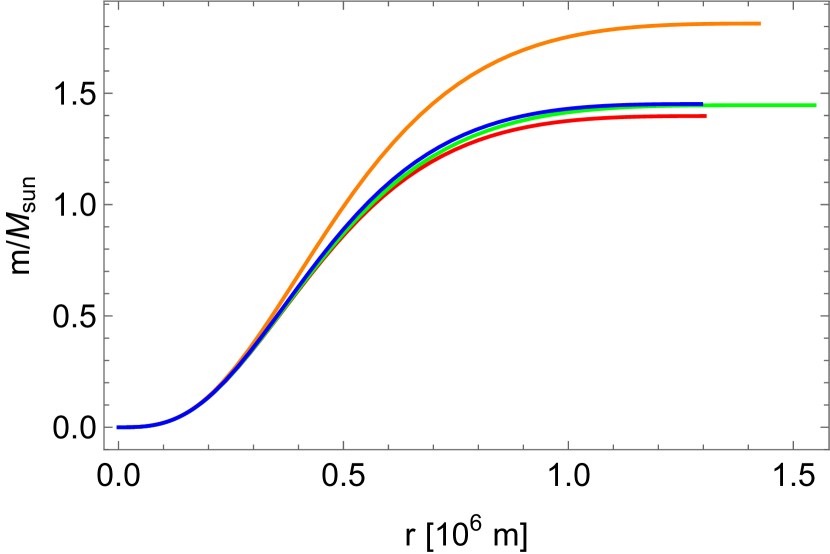
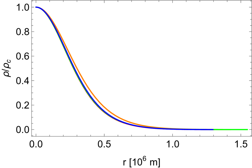
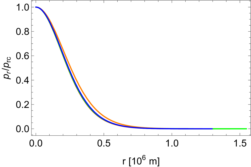
Figure 1: Mass function $m(r)$, energy density $\rho(r)$, radial pressure $p_{\text{r}}(r)$ versus radius $r$. Parameter values: $\alpha=0,\beta=0,\kappa=0$ for red, $\alpha=0.4,\beta=0,\kappa=0$ for orange, $\alpha=0,\beta=-4\times 10^{-4},\kappa=0$ for green, $\alpha=0,\beta=0,\kappa=10$ for blue. $\rho_{\text{c}}$ and $p_{\text{rc}}$ represent the density and radial pressure at the center of the sphere, respectively. $M_{\text{sun}}$ stands for the mass of the sun. In the two images on the right, the red line overlaps the blue one so badly that it is barely visible.

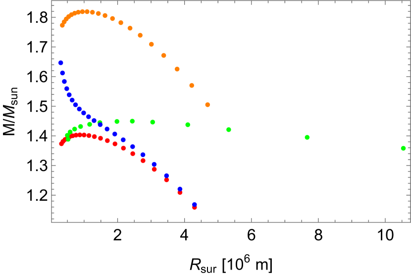
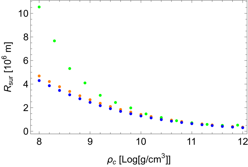
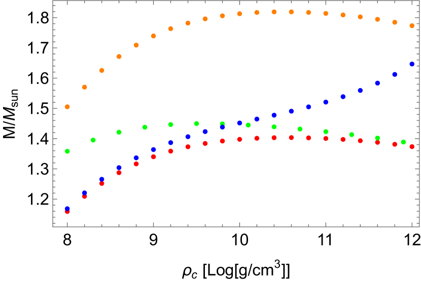
Figure 2: Relationship among total mass $M$ (up to surface), surface radius $R_{\text{sur}}$, logarithm of center density $\log(\rho_{\text{c}})$. Parameter values: $\alpha=0,\beta=0,\kappa=0$ for red, $\alpha=0.4,\beta=0,\kappa=0$ for orange, $\alpha=0,\beta=-4\times 10^{-4},\kappa=0$ for green, $\alpha=0,\beta=0,\kappa=10$ for blue. In the middle image, the red dotted line overlaps the blue one so badly that it is barely visible.

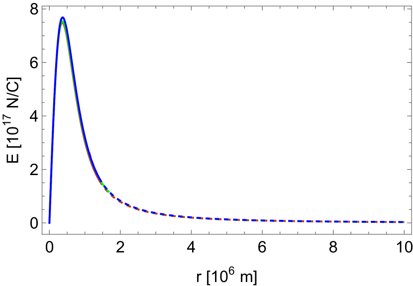
Figure 3: The distributions of the charge function $q(r)$ and the electric field $E(r)$. Parameter values: $\alpha=0.4,\beta=0,\kappa=0$ for red, $\alpha=0.4,\beta=-4\times 10^{-4},\kappa=0$ for green, $\alpha=0.4,\beta=0,\kappa=10$ for blue. In the second graph the three curves are very close to each other. It can be seen that the electric field is almost independent of the other parameters.

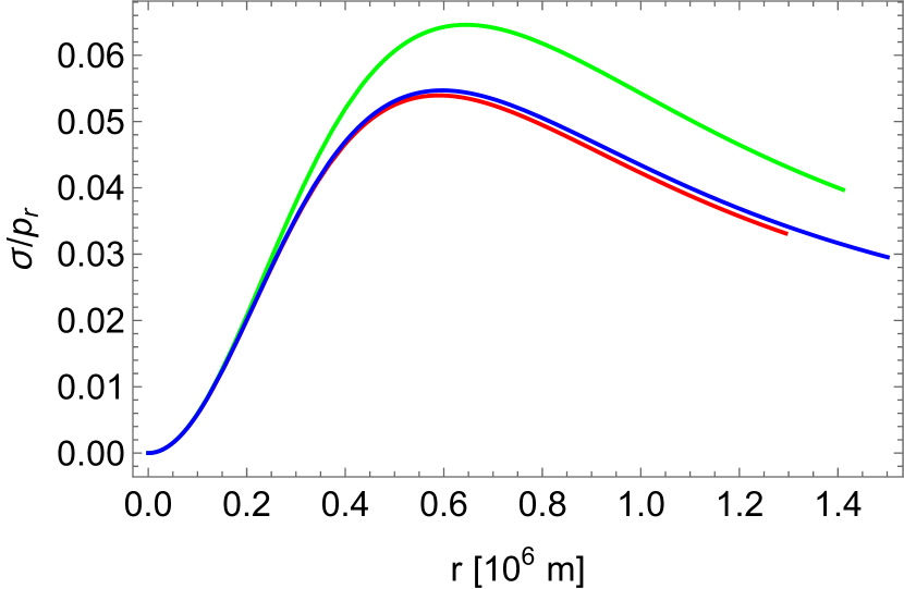
Figure 4: The distribution of the measure of relative anisotropy $\sigma/p_{\text{r}}$. Parameter values: $\alpha=0,\beta=0,\kappa=10$ for red, $\alpha=0.4,\beta=0,\kappa=10$ for green, $\alpha=0,\beta=-4\times 10^{-4},\kappa=10$ for blue. Deviations from anisotropy are less sensitive to modify gravity than charging.

V conclusions

In this paper, the physical properties of charged white dwarfs with anisotropic pressure under $f(R,T)$ gravity are investigated. The gravitational field action in $f(R,T)$ gravity is a more general function compared to GR. Considering the WD as a ball composed of degenerate electron gas, I use Chandrasekhar EoS. It originally described the relationship between isotropic pressure and density, but is considered radial pressure in this paper. In addition, it is assumed that the charge density distribution is proportional to the energy density, thus finally obtaining the basic characteristics of the WD structure.

After obtaining the modified TOV equations, numerical solutions are found under appropriate spherical center boundary conditions. By changing different parameter values, the effects of different aspects on the stars are compared. Under different combinations of several typical parameters, various scenarios were studied separately: (i) mass function $m(r)$, energy density $\rho(r)$, radial pressure $p_{\text{r}}(r)$ versus radius $r$; (ii) the relations among total mass (up to surface) $M$, surface radius $R_{\text{sur}}$, logarithm of center density $\log(\rho)$ (iii) the distributions of the charge function $q(r)$ and the electric field $E(r)$; (iv) the distribution of the measure of relative anisotropy $\sigma/p_{\text{r}}$. A brief interpretive analysis of the results in each case was performed.

The advantage of using $f(R,T)=R+2\beta T$ is that its form is computationally convenient while guaranteeing that modified gravitational effects can be represented. This model goes straight back to standard GR theory outside the star. More complex models are involved in the general $f(R)$ and $f(R,T)$ theories. The author has tried to discuss a more complicated model $f(R,T)=R+2\beta T+\gamma RT$ to analyze more complex matter-gravity coupling. Its analytical derivation is similar to the procedure in this paper, but some problems from the high order are encountered when seeking numerical solutions. There are also authors trying $f(R,T)=R+2\beta T+\gamma T^{2}$ model and $f(R,T,R_{ab}T^{ab})$ gravity[30, 31, 32], and got interesting results.

Again, it is emphasized that the charge density distribution considered in this paper is proportional to the matter energy density, which is not necessarily the best WD model. Other authors suggested that the charge density distribution of WD has a Gaussian distribution centered on the surface[25, 12], and eventually got their results as well. It must also be noted that the gravitational model in this work has been under discussion in recent years. Some arguments can be found in [33, 34, 35].

Appendix A Non-zero components of several important tensors

$$\mathcal{M}_{00} =\rho\mathrm{e}^{2\psi}, \mathcal{M}_{11} =p_{\text{r}}\mathrm{e}^{2\lambda}$$ (26)

$$\mathcal{M}_{22} =p_{\text{t}}r^{2}, \mathcal{M}_{33} =p_{\text{t}}r^{2}\sin^{2}\theta$$

$$\Theta_{00} =-(p_{\text{t}}+2\rho)\mathrm{e}^{2\psi}, \Theta_{11} =(p_{\text{t}}-2p_{\text{r}})\mathrm{e}^{2\psi}$$ (27)

$$\Theta_{22} =-p_{\text{t}}r^{2}, \Theta_{33} =-p_{\text{t}}r^{2}\sin^{2}\theta$$

$$\mathcal{E}_{00} =\mathrm{e}^{2\psi}\times q^{2}/8\pi r^{4}, \mathcal{E}_{11} =-\mathrm{e}^{2\lambda}\times q^{2}/8\pi r^{4}$$ (28)

$$\mathcal{E}_{22} =r^{2}\times q^{2}/8\pi r^{4}, \mathcal{E}_{33} =r^{2}\sin^{2}\theta\times q^{2}/8\pi r^{4}$$

References

- Bennett et al. [2003] C. L. Bennett, M. Halpern, G. Hinshaw, N. Jarosik, A. Kogut, M. Limon, S. S. Meyer, L. Page, D. N. Spergel, G. S. Tucker, E. Wollack, E. L. Wright, C. Barnes, M. R. Greason, R. S. Hill, E. Komatsu, M. R. Nolta, N. Odegard, H. V. Peiris, L. Verde, and J. L. Weiland, First-Year Wilkinson Microwave Anisotropy Probe (WMAP)* Observations: Preliminary Maps and Basic Results, The Astrophysical Journal Supplement Series 148, 1 (2003).
- Spergel et al. [2003] D. N. Spergel, L. Verde, H. V. Peiris, E. Komatsu, M. R. Nolta, C. L. Bennett, M. Halpern, G. Hinshaw, N. Jarosik, A. Kogut, M. Limon, S. S. Meyer, L. Page, G. S. Tucker, J. L. Weiland, E. Wollack, and E. L. Wright, First-Year Wilkinson Microwave Anisotropy Probe (WMAP)* Observations: Determination of Cosmological Parameters, The Astrophysical Journal Supplement Series 148, 175 (2003).
- Spergel et al. [2007] D. N. Spergel, R. Bean, O. Dore, M. R. Nolta, C. L. Bennett, J. Dunkley, G. Hinshaw, N. Jarosik, E. Komatsu, L. Page, H. V. Peiris, L. Verde, M. Halpern, R. S. Hill, A. Kogut, M. Limon, S. S. Meyer, N. Odegard, G. S. Tucker, J. L. Weiland, E. Wollack, and E. L. Wright, Three-Year Wilkinson Microwave Anisotropy Probe (WMAP) Observations: Implications for Cosmology, The Astrophysical Journal Supplement Series 170, 377 (2007).
- Glavan and Lin [2019] D. Glavan and C. Lin, Einstein-Gauss-Bonnet gravity in 4-dimensional space-time, Phys. Rev. Lett. 124, 081301 (2020) 10.1103/PhysRevLett.124.081301 (2019), arXiv:1905.03601 [gr-qc] .
- Shankaranarayanan and Johnson [2022] S. Shankaranarayanan and J. P. Johnson, Modified theories of Gravity: Why, How and What?, General Relativity and Gravitation 54, https://doi.org/10.1007/s10714-022-02927-2 (2022), arXiv:2204.06533 [gr-qc] .
- Sotiriou and Faraoni [2010] T. P. Sotiriou and V. Faraoni, theories of gravity, Reviews of Modern Physics 82, 451 (2010).
- Felice and Tsujikawa [2010] A. D. Felice and S. Tsujikawa, Theories, Living Reviews in Relativity 13, 10.12942/lrr-2010-3 (2010).
- Starobinsky [1980] A. Starobinsky, A new type of isotropic cosmological models without singularity, Physics Letters B 91, 99 (1980).
- Pretel and Duarte [2022] J. M. Z. Pretel and S. B. Duarte, Anisotropic quark stars in gravity, Class. Quantum Grav. 39 (2022) 155003 10.1088/1361-6382/ac7a88 (2022), arXiv:2202.04467 [gr-qc] .
- Harko et al. [2011] T. Harko, F. S. N. Lobo, S. Nojiri, and S. D. Odintsov, gravity, Physical Review D 84, 024020 (2011).
- Carvalho et al. [2017] G. A. Carvalho, R. V. Lobato, P. H. R. S. Moraes, J. D. V. Arbañil, R. M. M. Jr, E. Otoniel, and M. Malheiro, Stellar equilibrium configurations of white dwarfs in the gravity, The European Physical Journal C 77, 10.1140/epjc/s10052-017-5413-5 (2017), arXiv:1706.03596 [gr-qc] .
- Rocha et al. [2019] F. Rocha, G. A. Carvalho, D. Deb, and M. Malheiro, Study of the charged super-chandrasekhar limiting mass white dwarfs in the gravity, Phys. Rev. D 101, 104008 (2020) 10.1103/PhysRevD.101.104008 (2019), arXiv:1911.08894 [physics.gen-ph] .
- Deb et al. [2018] D. Deb, S. V. Ketov, M. Khlopov, and S. Ray, Study on charged strange stars in gravity, Journal of Cosmology and Astroparticle Physics 2019 (10), 070, arXiv:1812.11736 [gr-qc] .
- Sharif and Waseem [2018a] M. Sharif and A. Waseem, Anisotropic quark stars in gravity, The European Physical Journal C 78, 10.1140/epjc/s10052-018-6363-2 (2018a).
- Biswas et al. [2020] S. Biswas, D. Shee, B. K. Guha, and S. Ray, Anisotropic strange star with Tolman–Kuchowicz metric under gravity, The European Physical Journal C 80, 10.1140/epjc/s10052-020-7725-0 (2020).
- Biswas et al. [2021] S. Biswas, D. Deb, S. Ray, and B. Guha, Anisotropic charged strange stars in Krori-Barua spacetime under gravity, Annals of Physics 428, 168429 (2021).
- Rej and Bhar [2021] P. Rej and P. Bhar, Charged strange star in gravity with linear equation of state, Astrophysics and Space Science 366, 35 (2021) 10.1007/s10509-021-03943-5 (2021), arXiv:2105.12572 [gr-qc] .
- Rej et al. [2021] P. Rej, P. Bhar, and M. Govender, Charged compact star in gravity in Tolman-Kuchowicz spacetime, The European Physical Journal C 81, 316 (2021).
- Pretel et al. [2022] J. M. Z. Pretel, T. Tangphati, A. Banerjee, and A. Pradhan, Charged quark stars in gravity, Chinese Phys. C 46 (2022) 115103 10.1088/1674-1137/ac84cb (2022), arXiv:2207.12947 [gr-qc] .
- Chandrasekhar [1931] S. Chandrasekhar, The Maximum Mass of Ideal White Dwarfs, The Astrophysical Journal 74, 81 (1931).
- Howell et al. [2006] D. A. Howell, M. Sullivan, P. E. Nugent, R. S. Ellis, A. J. Conley, D. L. Borgne, R. G. Carlberg, J. Guy, D. Balam, S. Basa, D. Fouchez, I. M. Hook, E. Y. Hsiao, J. D. Neill, R. Pain, K. M. Perrett, and C. J. Pritchet, The type Ia supernova SNLS-03D3bb from a super-Chandrasekhar-mass white dwarf star, Nature 443, 308 (2006).
- Scalzo et al. [2010] R. A. Scalzo, G. Aldering, P. Antilogus, C. Aragon, S. Bailey, C. Baltay, S. Bongard, C. Buton, M. Childress, N. Chotard, Y. Copin, H. K. Fakhouri, A. Gal-Yam, E. Gangler, S. Hoyer, M. Kasliwal, S. Loken, P. Nugent, R. Pain, E. Pécontal, R. Pereira, S. Perlmutter, D. Rabinowitz, A. Rau, G. Rigaudier, K. Runge, G. Smadja, C. Tao, R. C. Thomas, B. Weaver, and C. Wu, NEARBY SUPERNOVA FACTORY OBSERVATIONS OF SN 2007if: FIRST TOTAL MASS MEASUREMENT OF A SUPER-CHANDRASEKHAR-MASS PROGENITOR, The Astrophysical Journal 713, 1073 (2010).
- Chandrasekhar [1935] S. Chandrasekhar, The Highly Collapsed Configurations of a Stellar Mass. (Second Paper.), Monthly Notices of the Royal Astronomical Society 95, 207 (1935).
- Liu et al. [2014] H. Liu, X. Zhang, and D. Wen, One possible solution of peculiar type Ia supernovae explosions caused by a charged white dwarf, Physical Review D 89, 104043 (2014).
- Carvalho et al. [2018] G. A. Carvalho, J. D. V. Arbañil, R. M. Marinho, and M. Malheiro, White dwarfs with a surface electrical charge distribution: equilibrium and stability, The European Physical Journal C 78, 10.1140/epjc/s10052-018-5901-2 (2018).
- Negreiros et al. [2009] R. P. Negreiros, F. Weber, M. Malheiro, and V. Usov, Electrically charged strange quark stars, Physical Review D 80, 083006 (2009).
- Pretel et al. [2021] J. M. Pretel, S. E. Jorás, R. R. Reis, and J. D. Arbañil, Radial oscillations and stability of compact stars in gravity, Journal of Cosmology and Astroparticle Physics 2021 (04), 064.
- Sharif and Siddiqa [2018] M. Sharif and A. Siddiqa, Equilibrium configurations of anisotropic polytropes in gravity, The European Physical Journal Plus 133, 10.1140/epjp/i2018-12060-8 (2018).
- Maurya and Tello-Ortiz [2020] S. Maurya and F. Tello-Ortiz, Charged anisotropic compact star in gravity: A minimal geometric deformation gravitational decoupling approach, Physics of the Dark Universe 27, 100442 (2020).
- Sharif and Waseem [2016] M. Sharif and A. Waseem, Physical behavior of anisotropic compact stars in gravity, Canadian Journal of Physics 94, 1024 (2016).
- Sharif and Waseem [2018b] M. Sharif and A. Waseem, Role of Model on Anisotropic Polytropes, Int. J. Mod. Phys. D 27(2018)1950007 10.1142/S021827181950007X (2018b), arXiv:1812.11037 [gr-qc] .
- Sharif and Naseer [2021] M. Sharif and T. Naseer, Effects of gravity on anisotropic charged compact structures, Chinese Journal of Physics 73, 179 (2021).
- Fisher and Carlson [2019] S. B. Fisher and E. D. Carlson, Reexamining gravity, Physical Review D 100, 064059 (2019).
- Harko and Moraes [2020] T. Harko and P. H. Moraes, Comment on “Reexamining gravity”, Physical Review D 101, 108501 (2020).
- Fisher and Carlson [2020] S. B. Fisher and E. D. Carlson, Reply to “Comment on ‘Reexamining gravity’”, Physical Review D 101, 108502 (2020).