Optical properties of the solar gravity lens

Abstract

It is well known that the solar gravitational field can be considered as a telescope with a prime focus at locations beyond 550 au. In this work we present a new derivation of the wave-optical properties of the system, by adapting the arrival-time formalism from gravitational lensing. At the diffraction limit the angular resolution is similar to that of a notional telescope with the diameter of the Sun, and the maximum light amplification is $8\pi^{4}GM_{\odot}/(c^{2}\lambda)$, enough to detect a $1\,$W laser on Proxima Centauri b pointed in the general direction of the Sun. Extended sources, however, would be blurred by the wings of the point spread function into the geometrical-optics regime of gravitational lensing. Broad-band sources would have to further contend with the solar corona. Imaging an exoplanet surface as advocated in the literature, without attempting to reach the diffraction limit, appears achievable. For diffraction-limited imaging (sub-km scales from 100 pc) nearby neutron stars appear to be most plausible targets.

1 Introduction

The phenomenon of light taking multiple paths through a gravitational field is now a familiar one. Small bright sources can produce two or more discrete images when gravitationally lensed, as in the original double quasar (discovered by Walsh et al., 1979). Extended sources when similarly lensed produce arcs, which may blend nearly into rings, for example the “Cosmic Horseshoe” (discovered by Belokurov et al., 2007). Such systems are all in the regime of geometrical optics; there is no optical interference between the separate light paths. The reason interference does not occur is that the light paths differ in travel time by hours to years, which is much longer than the coherence time of the light source. Scenarios where interference in gravitational lensing could occur have been studied (e.g., Jow et al., 2020; Ramesh et al., 2021) but are not observable yet.

There is, however, another way to see interference in gravitational lensing, albeit a futuristic one. It involves using the Sun as the lens, by sending an observer spacecraft to a distance $d_{OL}$ such that the angular radius $R_{\odot}/d_{OL}$ of the Sun becomes smaller than the deflection angle $4GM_{\odot}/(c^{2}R_{\odot})$ at the rim of the Sun. A light source precisely behind the Sun will then be lensed into a diffracting ring, resulting in a real image with a point spread function. The required distance is $d_{OL}\geq$550\text{\,}\mathrm{a}\mathrm{u}$$ or about three light days. In the same year as the first gravitational lens discovery and the first Saturn flyby Eshleman (1979), combining the fascinations of gravitational lensing and deep-space missions, drew attention to both the great potential and the formidable problems of a mission to the solar gravity focus. Subsequently several other authors, notably Maccone (2010) and recently Turyshev et al. (2020) have advocated a solar gravity lens mission. The wave optics of the solar gravitational lens has also been studied in several works (Herlt & Stephani, 1976; Deguchi & Watson, 1986; Nakamura & Deguchi, 1999; Nambu, 2013; Turyshev, 2017; Turyshev & Toth, 2017).

In this paper we will re-derive the optical properties of the solar gravity lens in a simple way, by adapting the Fermat-principle formulation of gravitational lensing. This approach most resembles Nambu (2013), whereas most other works proceed by solving for a plane electromagnetic wave crossing a spherical gravitational field. We will then briefly discuss the expected photon fluxes from different kinds of targets, and compare with the foreground light from the solar corona. The approach used here is technically simpler, in that it involves a scalar quantity (essentially the optical path length) rather than the electromagnetic four-vector potential, but in doing so sacrifices information like polarisation, which is encoded in the four-potential.

We will not attempt to address any spacecraft or instrument issues. Turyshev et al. (2020) is a good summary of these. We will also not include two important issues relating to the Sun. One is possible decoherence caused by the solar corona; Turyshev & Toth (2019) find that the effect is negligible at optical wavelengths. The other is perturbations due to the Sun’s oblateness and higher multipoles; this actually a significant effect (cf. Loutsenko, 2018; Turyshev & Toth, 2021d), which we will discuss briefly later, but for the present work we assume a spherical Sun.

2 Lensing time delays

Consider a possible path for a photon travelling from a source to a point in the camera plane. The path first goes in a straight line to a point $(R,\Phi)$ in a plane through the sun parallel to the camera plane; then it changes direction and takes a straight route to the point $(r,\phi)$ in the camera plane. Fig. 1 shows the geometry being considered, omitting $\Phi$ and $\phi$ for simplicity. It is the same as in the well-known formulation of Fermat’s principle in gravitational lensing by Blandford & Narayan (1986) except that source and observer have been swapped. From Eqs. 2.1–2.6 of that paper, the arrival time

$$t(\theta_{I},\theta_{S})=\frac{d_{SL}d_{SO}}{2cd_{LO}}(\theta_{I}-\theta_{S})^{2}-4\frac{GM_{\odot}}{c^{3}}\ln\theta_{I}$$ (1)

follows, assuming the angles

$$\theta_{I}=\frac{R}{d_{SL}}\qquad\theta_{S}=\frac{r}{d_{SO}}$$ (2)

are small. Blandford & Narayan (1986) also include dependence on redshifts in an expanding universe, which can be disregarded here.

Including the angles $\Phi$ and $\phi$ we have

$$t(r,\phi,R,\Phi) =\frac{\eta r^{2}+\eta^{-1}R^{2}-2rR\cos(\Phi-\phi)}{2c\,d_{LO}}$$ (3)

$$-\frac{2R_{S}}{c}\,\ln\left(R/d_{SL}\right)$$

where

$$R_{S}=\frac{2GM_{\odot}}{c^{2}}$$ (4)

is the nominal Schwarzschild radius, and the distance ratio $d_{SL}/d_{SO}$ is denoted by $\eta$. For sources of interest, $d_{SL}\gg d_{LO}$ and hence $\eta\approx 1$. We can eliminate $\eta$ by redefining $R$ and $r$ slightly, simplifying the arrival time to the following.

$$t(r,\phi,R,\Phi) =\frac{r^{2}+R^{2}-2rR\cos(\Phi-\phi)}{2c\,d_{LO}}$$ (5)

$$-\frac{2R_{S}}{c}\,\ln\left(R/d_{SL}\right)$$

Since we have assumed a spherical Sun, the dependence on $\Phi$ and $\phi$ is only through $\cos(\Phi-\phi)$. Departures from a spherical Sun will present a more complicated dependence (cf. Eq. 119 from Turyshev & Toth, 2021a).

To get an expression for the amplitude in the observer plane we need to sum up all virtual photon paths in the solar plane. This means we integrate the photon paths over the solar plane:

$$A(r,\phi)\propto\int e^{2\pi i\nu t(r,\phi,R,\Phi)}\,R\,dR\,d\Phi$$ (6)

This is the Fresnel-Kirchhoff diffraction integral for our problem.

To simplify the following derivation, it is useful to introduce

$$R_{E} =\sqrt{2R_{S}\,d_{LO}}$$ (7)

$$R_{F} =\sqrt{\lambda d_{LO}}$$

which are the Einstein radius and the Fresnel scale respectively. We now rewrite the phase as

$$2\pi\nu t(r,\phi,R,\Phi)=\frac{2\pi}{R_{F}^{2}}\Big{(} {\textstyle\frac{1}{2}}(r^{2}+R^{2})-rR\cos(\Phi-\phi)$$ (8)

$$-R_{E}^{2}\,\ln(R/d_{SL})\Big{)}$$

Fig. 2 illustrates the arrival time (8), without and with the last (lensing) term. The quantity shown is $\cos(2\pi\nu t)$ for $t(R,\Phi)$ at a fixed $r,\phi$ and a notional $\nu$ of $1\rm\,MHz$. A grey blur in the figure indicates $t$ varying quickly with $R,\phi$. Extended red or cyan regions in the figure indicates where $t$ is stationary or nearly stationary. In the absence of a lensing mass, the only stationary point of $t$ is a minimum, as evident in the upper panel. In the lower panel, a minimum and a saddle point are apparent. In geometrical optics, there are images (virtual images) at such stationary points of $t$. In wave optics, however, we need to integrate the complex amplitude over $R$ and $\Phi$.

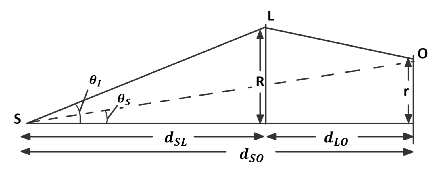
Figure 1: Distances and angles in gravitational lensing (adapted from Fig. 1 in Blandford & Narayan, 1986). The optical axis (horizonal line) runs from the source point through the centre of the lens to a reference point on the observer plane. A photon leaves the source at angle $\theta_{I}$ from the optical axis, gets deflected and delayed at radius $R$ of the lens, and reaches the observer plane at radius $r$, which is the spot where an unlensed photon leaving the source at $\theta_{S}$ would arrive. The angles $\theta_{I}$ and $\theta_{S}$ are understood as two-dimensional.

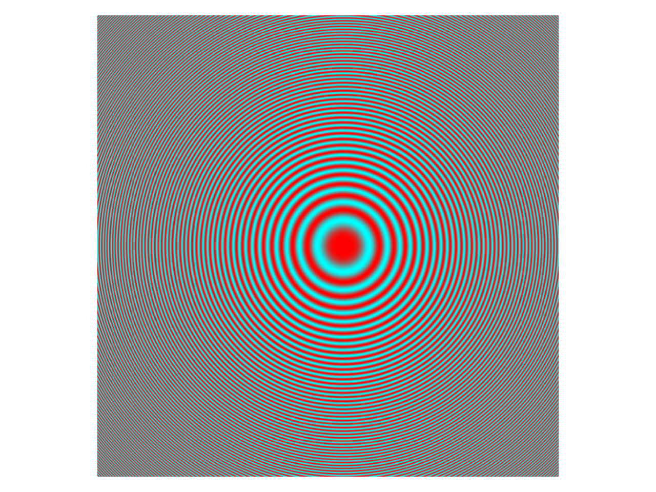
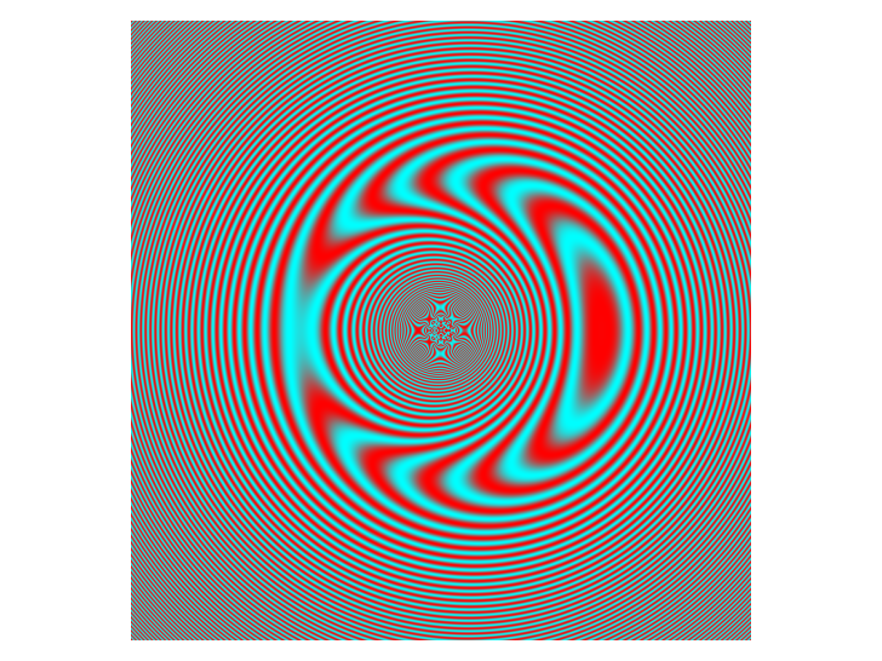
Figure 2: A representation of the phase in the observer’s sky with no lens (upper panel) and with the solar gravity lens (lower panel). The quantity shown is $\cos(2\pi\nu t)$ from Eq. (8), with red indicating $+1$, grey indicates 0, and cyan $-1$. In an animated version of the figure, where the phase keeps increasing with time, the pattern appears to travel from higher-$t$ regions to lower-$t$ regions. The observer is located at $r=$2\text{\times}{10}^{8}\text{\,}\mathrm{m}$$ from the focal line, and $R$ in the figure ranges from 0 to $1.4\text{\times}{10}^{9}\text{\,}\mathrm{m}$. The Einstein radius $R_{E}$ corresponds to the large ring in the lower panel. The Fresnel scale $R_{F}$ corresponds to the largest fringes. To make $R_{F}$ noticeable, we have used a very low frequency $\nu=1\rm\,MHz$. At optical wavelengths the Fresnel scale would be $\sim 10^{4}$ times smaller.

3 The point spread function

The phase in the integrand in (6) can be split up in a part of angular dependence and a part of radial dependence. We discard constants and dependencies on $r$ only, which contribute only constant phase. This leads to a split up integral for the amplitude:

$$A(r,\phi)\propto\int e^{i\psi(R)}R\,dR\,\int e^{-2\pi i(rR/R_{F}^{2})\cos(\Phi-\phi)}d\Phi$$ (9)

where

$$\psi(R)=\frac{2\pi}{R_{F}^{2}}\Big{(}{\textstyle\frac{1}{2}}R^{2}-R_{E}^{2}\ln(R/d_{OL})\Big{)}$$ (10)

Using the well-known integral for Bessel functions

$$J_{0}(u)=\frac{1}{2\pi}\int_{-\pi}^{\pi}e^{iu\cos(\Phi)}d\Phi$$ (11)

the double integral in (9) can be simplified to a single integral:

$$A(r)\propto\int e^{i\psi(R)}J_{0}\left(\frac{2\pi rR}{R_{F}^{2}}\right)\,R\,dR$$ (12)

Integration over $\Phi$ also removes the $\phi$ dependence, because only the difference $\Phi-\phi$ appears in the integrand in Eq. (9).

The phase (10) has a minimum at $R=R_{E}$. Since only the region of minimal phase change contributes to the image, we can approximate the phase function around its minimum in order to get a simpler expression. With a Taylor expansion the phase function (10) can be approximated around $R_{E}$:

$$\psi(R) =\psi(R_{E})+\psi^{\prime}(R_{E})(R-R_{E})$$ (13)

$$+{\textstyle\frac{1}{2}}\psi^{\prime\prime}(R_{E})(R-R_{E})^{2}+O((R-R_{E})^{3})$$

In (13) we note that $\psi^{\prime}(R_{E})=0$. Further, terms not depending on $r$ or $R$ can be ignored, since $\psi$ is a phase. In our case $O((R-R_{E})^{3})$ until $R=R_{E}\pm 20R_{F}$ is still about $10^{4}$ times smaller then the previous terms in the Taylor approximation. Since the region of $R$ we are integrating over is always within $R=R_{E}\pm 20R_{F}$ we can ignore $O((R-R_{E})^{3})$ and terms of higher order. The phase can then be approximated as

$$\psi(R)\approx 2\pi\frac{(R-R_{E})^{2}}{R_{F}^{2}}$$ (14)

We can take the terms that do not depend on $R$ out of the integral (12) and get:

$$A(r)\propto\int_{-\infty}^{\infty}e^{2\pi i\left(\frac{R-R_{E}}{R_{F}}\right)^{2}}J_{0}\left(\frac{2\pi rR}{R_{F}^{2}}\right)\,R\,dR$$ (15)

To find the light amplification $\mu$ we have to calculate

$$\mu=\left|\frac{A(r)}{A_{0}(r)}\right|^{2}$$ (16)

where $A_{0}(r)$ is the diffraction integral for the case of no lens. Here we cannot simply put $R=R_{E}$ in the expression (15) for $A(r)$, because the Taylor-approximated phase (14) is not valid for $R_{E}=0$. We have to go back to the earlier expression (12) and put $R_{E}=0$ there. This gives

$$A_{0}(r)\propto\int_{-\infty}^{\infty}e^{\pi i\left(\frac{R}{R_{F}}\right)^{2}}J_{0}\left(\frac{2\pi rR}{R_{F}^{2}}\right)\,R\,dR$$ (17)

We thus have

$$\frac{A(r)}{A_{0}(r)}=\frac{\int_{0}^{\infty}e^{2\pi i\left(\frac{R-R_{E}}{R_{F}}\right)^{2}}J_{0}\left(\frac{2\pi rR}{R_{F}^{2}}\right)\,R\,dR}{\int_{0}^{\infty}e^{\pi i\left(\frac{R}{R_{F}}\right)^{2}}J_{0}\left(\frac{2\pi rR}{R_{F}^{2}}\right)\,R\,dR}$$ (18)

In the numerator the integrand contributes significantly only near $R=R_{E}$, so we can take any slow $R$ dependence outside the integral. This lets us simplify to the following.

$$\frac{A(r)}{A_{0}(r)}={} \frac{2R_{E}}{R_{F}}\,J_{0}\!\left(\frac{2\pi rR_{E}}{R_{F}^{2}}\right)\times$$ (19)

$$\frac{\int_{0}^{\infty}e^{2\pi iu^{2}}\,du}{\int_{0}^{\infty}e^{\pi iu^{2}}J_{0}\!\left(\frac{2\pi ru}{R_{F}^{2}}\right)\,u\,du}$$

Substituting the standard integrals

$$\int_{0}^{\infty}e^{2\pi iu^{2}}\,du=(1+i)/4$$ (20)

$$\int_{0}^{\infty}e^{\pi iu^{2}}J_{0}(ku)\,u\,du=ie^{ik^{2}/(4\pi)}/(2\pi)$$

and simplifying gives the normalised light amplification

$$\mu=4\pi^{2}\frac{R_{S}}{\lambda}J_{0}^{2}\left(\frac{2\pi r}{\lambda}\frac{R_{E}}{d_{LO}}\right)$$ (21)

which, since it is a function of radius $r$ on the observer plane, can be considered a point spread function.

We can compare our result (21) with the expression in Eq. 135 of Turyshev & Toth (2017). Substituting $\rho\rightarrow r$, $r_{g}\rightarrow R_{S}$ and $z\rightarrow d_{LO}$ in their expression gives

$$\mu=\frac{4\pi^{2}R_{S}/\lambda}{1-e^{-4\pi^{2}R_{S}/\lambda}}J_{0}^{2}\left(\frac{2\pi r}{\lambda}\frac{R_{E}}{d_{LO}}\right)$$ (22)

The exponential function in (22) for typical wavelengths $\lambda$ in the visible spectrum is almost 0. So (22) simplifies to the same as (21).

4 The diffraction limit vs geometrical optics

If we look at a source plane instead of a point source, it is more useful to know the average amplification $\langle\mu\rangle$ of the whole observation area. For a circular source plane we can change the integral to polar coordinates and we find the average amplification as a function of the maximal radius $r_{1}$ in the observation plane.

$$\langle\mu\rangle_{r_{1}}=\frac{2\pi\int_{0}^{r_{1}}\mu(r)\,r\,dr}{\pi r_{1}^{2}}$$ (23)

Before inserting (21) in (23), the Bessel function in the former can be substituted by an approximation that is easier to integrate. For large argument $J_{0}$ can be approximated (see e.g., Brauer, 1963, Eq. 11) as

$$J_{0}(x)\approx\sqrt{\frac{2}{\pi x}}\cos{\left(x-\frac{\pi}{4}\right)}$$ (24)

We then insert (21) and (24) in (23) and simplify to get

$$\langle\mu\rangle_{r_{1}}=\frac{4R_{E}}{r_{1}^{2}}\int_{0}^{r_{1}}\cos^{2}{\left(\frac{2\pi r}{\lambda}\frac{R_{E}}{d_{LO}}-\frac{\pi}{4}\right)}\,dr$$ (25)

The integral in (25) can now be calculated analytically and gives us the resulting formula for the average amplification:

$$\langle\mu\rangle_{r_{1}}=\frac{2R_{E}}{r_{1}}+\frac{\lambda d_{LO}}{2\pi r_{1}^{2}}\left(1-\cos\left(\frac{4\pi r_{1}}{\lambda}\frac{R_{E}}{d_{LO}}\right)\right)$$ (26)

As we see, the amplification of extended sources tends to become independent of wavelength.

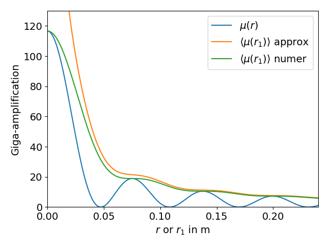
Figure 3: The point spread function and its enclosed averages. The plotted quantities are $\mu(r)$ from Eq. (21), and its enclosed average $\langle\mu(r_{1})\rangle$ as computed numerically from Eq. (23) and as estimated in Eq. (26).

Let us now change to angular terms. Let

$$\theta_{1}=\frac{r_{1}}{d_{LO}}=\frac{R_{1}}{d_{SL}}$$ (27)

be the angular radius of the source, and

$$\theta_{E}=\frac{R_{E}}{d_{LO}}$$ (28)

the angular Einstein radius. In terms of these, the diffraction limit is given by

$$J_{0}\left(\frac{2\pi R_{E}}{\lambda}\theta_{\lambda}\right)=0$$ (29)

$$\theta_{\lambda}=0.77\frac{\lambda}{2R_{E}}$$ (30)

Recall that an ordinary telescope has $J_{1}$ instead of $J_{0}$ in the condition (29).

For sources much larger than the diffraction limit but still small

$$\theta_{\lambda}\ll\theta_{1}\ll\theta_{E}$$ (31)

the mean amplification is

$$\langle\mu\rangle_{\theta_{1}}=\frac{2\theta_{E}}{\theta_{1}}$$ (32)

Now, for gravitational lensing by a star in geometrical-optics, there is a well-known expression for amplification that goes back to Einstein (1936)

$$\frac{1}{u}\frac{1+u^{2}/2}{\sqrt{1+u^{2}/4}}\quad\hbox{where}\quad u=\frac{\theta_{1}}{\theta_{E}}$$ (33)

Averaging over a disc of radius $\theta_{1}$ (assuming $\theta_{1}\ll\theta_{E}$) gives the same as Eq. (32).

Thus, as we might have expected, geometrical optics applies for sources much larger than the diffraction limit.

5 Foreground and background

If the Sun were dark, no further mirrors or lenses would be needed, a detector to gather light would be sufficient. Covering up the Sun, however, and letting through the light in the Einstein ring, necessitates a spacecraft telescope with some kind of coronograph.

The Sun from $600\text{\,}\rm\mathrm{a}\mathrm{u}$ has a spectral photon flux

$$\Phi_{\lambda}({\rm Sun})\approx$1\text{\times}{10}^{13}\text{\,}{\rm photons\;}\mathrm{s}^{-1}\mathrm{m}^{-2}\mathrm{n}\mathrm{m}^{-1}$$$ (34)

at $1\text{\,}\mathrm{\SIUnitSymbolMicro m}$. This is comparable to the brightness of the Moon as seen from the Earth, but over a very small area of $\sim$10\text{\,}\rm\mathrm{a}\mathrm{r}\mathrm{c}\mathrm{s}\mathrm{e}\mathrm{c}^{2}$$. Thus the optical setup would be very different from an ordinary coronograph, and more like the occulting masks developed for imaging extrasolar planets (see e.g., Beichman et al., 2020). We emphasise, however, that the idea is not to image the Einstein ring, but to let the amplitude through a narrow ring around $R_{E}$ interfere.

The width of the ring of light could be reduced to the diffraction limit of the observing telescope. Mission concepts envisage a 1 m telescope, which at optical wavelengths implies a ring of thickness $\approx 0.1^{\prime\prime}$. With $R_{E}\approx 2^{\prime\prime}$ the area of the ring would be about $1\text{\,}\rm\mathrm{a}\mathrm{r}\mathrm{c}\mathrm{s}\mathrm{e}\mathrm{c}^{2}$, or about a tenth of the area of the solar disc. Coming through this ring would be light from the solar corona. Close to the Sun, the surface brightness of the corona is a few times $10^{-6}$ that of the solar disc (November & Koutchmy, 1996). Thus suggests

$$\Phi_{\lambda}({\rm solar\ corona})\sim 10^{6}${\rm photons\;}\mathrm{s}^{-1}\mathrm{m}^{-2}\mathrm{n}\mathrm{m}^{-1}$$$ (35)

which is comparable to a bright star. The corona brightness itself could be subtracted out, but the shot noise from it will remain as a noise source, as will any intrinsic variation in the corona brightness.

The light ring will also let in some light from the night sky. That light will be lensed, but because lensing preserves surface brightness, the resulting photon flux will be the same as the unlensed night sky. The night sky brightness is $\approx$3\text{\times}{10}^{12}\text{\,}{\rm photons\;}\mathrm{m}^{-2}\mathrm{s}^{-1}\mathrm{sr}^{-1}$$ in a broad band (e.g., Table 1 from Preuß et al., 2002). Since $$1\text{\,}\rm\mathrm{a}\mathrm{r}\mathrm{c}\mathrm{s}\mathrm{e}\mathrm{c}^{2}$\simeq$2.5\text{\times}{10}^{-11}\text{\,}\rm\mathrm{s}\mathrm{r}$$ our assumed light ring will let in $\sim$10\text{\,}{\rm photons\;}\mathrm{s}^{-1}\mathrm{m}^{-2}$$ even in a broad band.

Thus the night-sky background is negligible, while the solar corona would be the principal limitation.

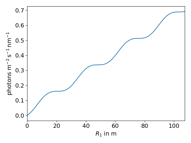
Figure 4: Observable photon flux at $1\text{\,}\mathrm{nm}$ from a uniform-brightness disc of radius $R_{1}$ at $1.3\text{\,}\rm\mathrm{p}\mathrm{c}$ emitting $1\text{\,}\mathrm{W}\mathrm{m}^{-2}\mathrm{n}\mathrm{m}^{-1}$.

6 Plausible targets

As potential targets, exoplanets in habitable zones immediately come to mind, especially well known being Proxima Centauri b at $1.3\,$pc (Anglada-Escudé et al., 2016), Teegarden b at $3.8\,$pc (Zechmeister et al., 2019), Trappist-1d at $12.1\,$pc (Gillon et al., 2016) and TOI 700 d at $31\,$pc (Gilbert et al., 2020). The last of these is a transiting system, and hence its orbital inclination is measured and its exact position can be predicted. The other three are inferred from radial-velocity perturbations of the host star, and their orbital inclinations are unknown. As a result, the location of the $r=0$ point on the observer plane has a large uncertainty. This problem could, however, be solved by preliminary direct imaging of the planet at the single-pixel level, which can be expected long before a 550 au mission becomes feasible.

The surface brightness of these exoplanets is not known, but $\sim$1\text{\,}\mathrm{W}\mathrm{m}^{-2}\mathrm{n}\mathrm{m}^{-1}$$ is a convenient round figure to assume for the spectral flux. The solar spectral irradiance in the visible range is close to this value (e.g., Gueymard, 2004). Converting to a photon rate and multiplying by the brightness factor (26) gives the observable spectral photon flux, say $\Phi_{\lambda}$ in ${\rm photons\;}\mathrm{s}^{-1}\mathrm{m}^{-2}\mathrm{n}\mathrm{m}^{-1}$. Fig. 4 shows the result at $1\text{\,}\mathrm{nm}$ for $d_{SL}=1.3\rm\,pc$ and $d_{LO}=600\rm\,au$. It is evident that even small bodies would yield non-zero photons.

The extended wings of the point spread function, and furthermore the bright foreground from the solar corona, would considerably degrade the achievable resolution of exoplanets, compared to the incredible $20\text{\,}\mathrm{m}$-scale on Proxima Centauri b suggested by Figs. 3 and 4. Toth & Turyshev (2021) carry out image deconvolution on a simulated Earth at the distance of Proxima, to a resolution of roughly $100\text{\,}\mathrm{km}$, and Turyshev & Toth (2022) consider deconvolution from 1200 au, where the solar corona is much fainter. Extrapolating from Fig. 4 we can estimate $\sim 10^{3}${\rm photons\;}\mathrm{s}^{-1}\mathrm{m}^{-2}\mathrm{n}\mathrm{m}^{-1}$$ from a 100 km pixel on Proxima Centauri b. Comparing with the foreground (35) we see that the exoplanet will be orders of magnitude fainter than the solar corona, but not that much fainter than the noise in the solar corona. These estimates, though of course only very rough, indicate that the solar corona would not prevent the imaging of exoplanets.

For imaging at the diffraction limit, the best prospect would be an isolated neutron star. The nearest of these (see e.g., Haberl, 2013) is RX J1856.5$-$3754, about $130\,$pc away. The distance is 100 times further than Proxima, but observing at a much shorter wavelength of say $100\text{\,}\mathrm{nm}$ would be desirable, giving a resolution of $\approx$200\text{\,}\mathrm{m}$$ at the diffraction limit.

Laser lines are interesting, because they could be observed in a very narrow band (say $0.01\text{\,}\mathrm{nm}$) thereby greatly reducing the foreground. Natural laser lines are known (in $\eta\,$Carinae, see Johansson & Letokhov, 2007) but why not artificial laser lines sent by interstellar friends? Various SETI scenarios have been discussed in Hippke (2018). Here we add one more.

Consider the first plateau in Fig. 4, which indicates the diffraction limit. This corresponds to a circular area of radius $R_{1}=$20\text{\,}\mathrm{m}$$ or about $1000\text{\,}\mathrm{m}^{2}$ on Proxima b. Over a bandwidth of $1\rm\,nm$, this area at its assumed brightness emits $1\rm\,kW$ of light and gives the observer $\sim$0.15\text{\,}{\rm photons}\;\mathrm{s}^{-1}\mathrm{m}^{-2}$$. Now imagine a $1\rm\,W$ laser with a milliradian dispersion, located anywhere inside this area, and aimed within a milliradian of the Sun. With the light within $10^{-6}\pi\rm\,sr$ rather than $2\pi\rm\,sr$ as with ordinary light, the laser would be equivalent to $2\rm\,MW$ of ordinary light emitted, and $\sim$300\text{\,}{\rm photons}\;\mathrm{s}^{-1}\mathrm{m}^{-2}$$ at the observer. Absent the foreground from the solar corona, this level of photon flux would be easily detectable. Through the solar corona, the laser would have to shine for some time, perhaps as short as $10\text{\,}\mathrm{s}$, to be detectable. There are complications arising from the small but non-zero asphericity of the Sun, which will spread the light out over a caustic pattern (Turyshev & Toth, 2021b, c), which we have not investigated, but it appears plausible that with the solar gravity lens, we could detect a laser pointer on Proxima Centauri b aimed towards the Sun. Provided of course, that we knew precisely where to look.

Data Availability

The code to generate the simulated data and figures are included in the supplementary material.

References

- Anglada-Escudé et al. (2016) Anglada-Escudé G., et al., 2016, Nature, 536, 437–440
- Beichman et al. (2020) Beichman C., et al., 2020, PASP, 132, 015002
- Belokurov et al. (2007) Belokurov V., et al., 2007, ApJ, 671, L9
- Blandford & Narayan (1986) Blandford R., Narayan R., 1986, ApJ, 310, 568
- Brauer (1963) Brauer F., 1963, The American Mathematical Monthly, 70, 954
- Deguchi & Watson (1986) Deguchi S., Watson W. D., 1986, Phys. Rev. D, 34, 1708
- Einstein (1936) Einstein A., 1936, Science, 84, 506
- Eshleman (1979) Eshleman V. R., 1979, Science, 205, 1133
- Gilbert et al. (2020) Gilbert E. A., et al., 2020, The Astronomical Journal, 160, 116
- Gillon et al. (2016) Gillon M., et al., 2016, Nature, 533, 221–224
- Gueymard (2004) Gueymard C. A., 2004, Solar Energy, 76, 423
- Haberl (2013) Haberl F., 2013, in Ness J. U., ed., The Fast and the Furious: Energetic Phenomena in Isolated Neutron Stars, Pulsar Wind Nebulae and Supernova Remnants. p. 6
- Herlt & Stephani (1976) Herlt E., Stephani H., 1976, International Journal of Theoretical Physics, 15, 45
- Hippke (2018) Hippke M., 2018, Acta Astronautica, 142, 64
- Johansson & Letokhov (2007) Johansson S., Letokhov V. S., 2007, New Astron. Rev., 51, 443
- Jow et al. (2020) Jow D. L., Foreman S., Pen U.-L., Zhu W., 2020, MNRAS, 497, 4956
- Loutsenko (2018) Loutsenko I., 2018, Progress of Theoretical and Experimental Physics, 2018
- Maccone (2010) Maccone C., 2010, Acta Astronautica, 67, 521
- Nakamura & Deguchi (1999) Nakamura T. T., Deguchi S., 1999, Progress of Theoretical Physics Supplement, 133, 137
- Nambu (2013) Nambu Y., 2013, International Journal of Astronomy and Astrophysics, 3, 1
- November & Koutchmy (1996) November L. J., Koutchmy S., 1996, ApJ, 466, 512
- Preuß et al. (2002) Preuß S., Hermann G., Hofmann W., Kohnle A., 2002, Nuclear Instruments and Methods in Physics Research A, 481, 229
- Ramesh et al. (2021) Ramesh R., Mena A. K., Bagla J. S., 2021, arXiv e-prints, p. arXiv:2109.09998
- Toth & Turyshev (2021) Toth V. T., Turyshev S. G., 2021, Phys. Rev. D, 103, 124038
- Turyshev (2017) Turyshev S. G., 2017, Phys. Rev. D, 95, 084041
- Turyshev & Toth (2017) Turyshev S. G., Toth V. T., 2017, Phys. Rev. D, 96, 024008
- Turyshev & Toth (2019) Turyshev S. G., Toth V. T., 2019, Phys. Rev. D, 99, 024044
- Turyshev & Toth (2021a) Turyshev S. G., Toth V. T., 2021a, Phys. Rev. D, 103, 064076
- Turyshev & Toth (2021b) Turyshev S. G., Toth V. T., 2021b, Phys. Rev. D, 104, 024019
- Turyshev & Toth (2021c) Turyshev S. G., Toth V. T., 2021c, Phys. Rev. D, 104, 044032
- Turyshev & Toth (2021d) Turyshev S. G., Toth V. T., 2021d, Phys. Rev. D, 104, 124033
- Turyshev & Toth (2022) Turyshev S. G., Toth V. T., 2022, MNRAS, 515, 6122
- Turyshev et al. (2020) Turyshev S. G., et al., 2020, arXiv e-prints, p. arXiv:2002.11871
- Walsh et al. (1979) Walsh D., Carswell R. F., Weymann R. J., 1979, Nature, 279, 381
- Zechmeister et al. (2019) Zechmeister M., et al., 2019, Astronomy & Astrophysics, 627, A49