Higher-order Monte Carlo through cubic stratification

Abstract

We propose two novel unbiased estimators of the integral $\int_{[0,1]^{s}}f(u)\mathrm{d}\mathrm{u}$ for a function $f$, which depend on a smoothness parameter $r\in\mathbb{N}$. The first estimator integrates exactly the polynomials of degrees $p<r$ and achieves the optimal error $n^{-1/2-r/s}$ (where $n$ is the number of evaluations of $f$) when $f$ is $r$ times continuously differentiable. The second estimator is also optimal in term of convergence rate and has the advantage to be computationally cheaper, but it is restricted to functions that vanish on the boundary of $[0,1]^{s}$. The construction of the two estimators relies on a combination of cubic stratification and control variates based on numerical derivatives. We provide numerical evidence that they show good performance even for moderate values of $n$.

1 Introduction

1.1 Background

This paper is concerned with the construction of unbiased estimators of the integral $\mathcal{I}(f):=\int_{[0,1]^{s}}f(u)\mathrm{d}\mathrm{u}$ based on a certain number $n$ of evaluations of $f$. The motivation for this problem is well-known. Many quantities of interest in applied mathematics may be expressed as such an integral. Providing random, unbiased approximations present several practical advantages. First, it greatly facilitates the assessment of the numerical error, through repeated runs. Second, such independent estimates may be generated in parallel, and then may be averaged to obtain a lower variance approximation of $\mathcal{I}(f)$. Third, generating unbiased estimates as plug-in replacements is of interest in various advanced Monte Carlo methodologies, such as pseudo-marginal sampling Andrieu and Roberts, (2009), stochastic approximation Robbins and Monro, (1951) and stochastic gradient descent. Finally, random integration algorithms converge at a faster rate than deterministic ones Novak, (1988) (but note that these convergence rates correspond to different criteria).

The most basic and well-known stochastic integration rule is the crude Monte Carlo method, where one simulates uniformly $n$ independent and identically distributed variates $U_{i}$, and returns $n^{-1}\sum_{i=1}^{n}f(U_{i})$ as an estimate of $\mathcal{I}(f)$. Assuming that $f\in L_{2}([0,1]^{s})$, the root mean square error (RMSE) of this estimator converges to zero at rate $n^{-1/2}$. In this paper we consider the problem of estimating $\mathcal{I}(f)$ under the additional condition that all the partial derivatives of $f$ of order less or equal to $r$ exist and are continuous, or, in short, that $f\in\mathcal{C}^{r}([0,1]^{s})$. Under this assumption on $f$ it is well-known that we can improve upon the crude Monte Carlo error rate. More precisely, for $f\in\mathcal{C}^{r}([0,1]^{s})$ the optimal convergence rate for the RMSE of an estimate $\widehat{\mathcal{I}}(f)$ of $\mathcal{I}(f)$ based on $n$ evaluations of $f$ is $n^{-1/2-r/s}$, in the sense that if $g:\mathbb{N}\rightarrow[0,\infty)$ is such that

$$\forall f\in\mathcal{C}^{r}\left([0,1]^{s}\right),n\geq 1,\quad\mathbb{E}\left[|\widehat{\mathcal{I}}(f)-\mathcal{I}(f)|^{2}\right]^{1/2}\leq g(n)\|f\|_{r}$$

(where $\|f\|_{r}$ is a bound on the $r$-th order derivatives of $f$, see Section 1.4 for a proper definition) then we must have $n^{-1/2-r/s}/g(n)=\mathcal{O}(1)$ (this result can for instance be obtained from Propositions 1-2 given in Section 2.2.4, page 55, of Novak, (1988)).

Stochastic algorithms that achieve this optimal convergence rate for $f\in\mathcal{C}^{r}([0,1]^{s})$ have been proposed e.g. in Haber, (1966) for $r=1$ and in Haber, (1967) for $r\in\{1,2\}$. In Haber, (1969) it is shown that if $\widehat{\mathcal{I}}(\cdot)$ is a stochastic quadrature (SQ) of degree $r-1$, that is, if $\mathbb{E}[\widehat{\mathcal{I}}(f)]=\mathcal{I}(f)$ for all $f\in L_{1}([0,1]^{s})$ and $\mathbb{P}(\widehat{\mathcal{I}}(f)=\mathcal{I}(f))=1$ if $f$ is a polynomial of degree $p<r$, then $\widehat{\mathcal{I}}(\cdot)$ can be used to define an estimator of $\mathcal{I}(f)$ whose RMSE converges to zero at rate $n^{-1/2-r/s}$ when $f\in\mathcal{C}^{r}([0,1]^{s})$. In Haber, (1969) a formula for a SQ of degree $r-1$ is given for $r\in\{3,4\}$ while, for $s=1$, Siegel and O’Brien, (1985) provides a SQ of degree $2r+1$ for all $r\geq 1$. For multivariate integration problems, and an arbitrary value of $r\geq 1$, a SQ of degree $r-1$ can be constructed from the integration method proposed in Ermakov and Zolotukhin, (1960). However, the algorithm proposed in this reference requires to perform a sampling task which is so computationally expensive that it is considered as almost intractable Patterson, (1987).

A related approach is derived by Dick in Dick, (2011), which achieves rate $\mathcal{O}(n^{-1/2-\alpha+\varepsilon})$ for $\varepsilon>0$ and a certain class of functions indexed by $\alpha$ (which differs from $\mathcal{C}^{r}\left([0,1]^{s}\right)$ even when $r=s\alpha$). We will go back to this point and compare our approach to Dick’s in our numerical study.

1.2 Motivation and plan

The paper is structured as follows. We introduce in Section 2 an unbiased estimator of $\mathcal{I}(f)$ which has the following three appealing properties when $f\in\mathcal{C}^{r}([0,1]^{s})$. First, its RMSE converges to zero at the optimal $n^{-1/2-r/s}$ rate. Second, it integrates exactly $f$ if $f$ is a polynomial of degree $p<r$. Third, for some constant $C<\infty$ and with probability one, the absolute value of its estimation error is bounded by $Cn^{-r/s}$, where $n^{-r/s}$ is the optimal convergence rate for a deterministic integration rule (this result can for instance be obtained from Proposition 1.3.5, page 28, of Novak, (1988)). In addition, we establish a central limit theorem (CLT) for a particular version of the proposed estimator. To the best of our knowledge, a CLT for an estimator of $\mathcal{I}(f)$ having an RMSE that converges at the optimal rate when $f\in\mathcal{C}^{r}([0,1]^{s})$ exists only for $r=1$ (see Bardenet and Hardy, (2020)).

In Section 3, we focus our attention on the estimation of $\mathcal{I}(f)$ when $f\in\mathcal{C}^{r}_{0}([0,1]^{s})$, where we define $\mathcal{C}^{r}_{0}([0,1]^{s})$ as the set of functions in $\mathcal{C}^{r}([0,1]^{s})$ whose partial derivatives of order $o\leq r$ are all equal to zero on the boundary of $[0,1]^{s}$. As we explain in that section, this set-up is particularly relevant for solving integration problems on $\mathbb{R}^{s}$. Restricting our attention to $\mathcal{C}^{r}_{0}([0,1]^{s})\subset\mathcal{C}^{r}([0,1]^{s})$ allows us to derive an estimator of $\mathcal{I}(f)$, referred to as the vanishing estimator in what follows, which is computationally cheaper than the previous estimator, while retaining its convergence properties, namely an RMSE of size $\mathcal{O}(n^{-1/2-r/s})$ and an actual error of size $\mathcal{O}(n^{-r/s})$ almost surely. We note that these convergence rates are optimal for integrating a function in $\mathcal{C}^{r}_{0}([0,1]^{s})$ (again, see Sections 1.3.5 and 2.2.4 of Novak, (1988)) and that an algorithm considering a similar class of functions is proposed in Krieg and Novak, (2017). The algorithm derived in this latter reference has the advantage to achieve the optimal aforementioned convergence rates for any $r\in\mathbb{N}$ but its implementation at reasonable computational cost remains an open problem.

Section 4 discusses some practical details about the proposed estimators, regarding on how their variance may be estimated and how the order of the vanishing estimator may be selected automatically. Section 5 presents numerical experiments which confirm that the estimators converge at the expected rates, and show that they are already practical for moderate values of $n$. Section 6 discusses future work. Proofs of certain technical lemmas are deferred to Appendix C.

1.3 Connection with function approximation

As noted by e.g. Novak, (2016), there is a strong connection between (unbiased) integration and function approximation. If one is able to construct an optimal approximation $\mathcal{A}_{n}(f)$ of $f\in\mathcal{C}^{r}{([0,1]^{s})}$, that is $\|f-\mathcal{A}_{n}(f)\|_{\infty}=\mathcal{O}(n^{-r/s})$ (see Novak, (1988), page 36) then one may derive the following unbiased estimate of $\mathcal{I}(f)$

$$\widehat{\mathcal{I}}(f):=\mathcal{I}\left(\mathcal{A}_{n}(f)\right)+\frac{1}{n}\sum_{i=1}^{n}\left(f-\mathcal{A}_{n}(f)\right)(U_{i}),\quad U_{i}\stackrel{{\scriptstyle\mathclap{\mbox{\tiny{iid}}}}}{{\sim}}\mathcal{U}([0,1]^{s})$$ (1)

which is also optimal, in the sense that its RMSE is $\mathcal{O}(n^{-1/2-r/s})$ for estimating $\mathcal{I}(f)$.

The (non-vanishing) estimator proposed in this paper for integrating a function $f\in\mathcal{C}^{r}{([0,1]^{s})}$ is to some extent related to this idea, with $\mathcal{A}_{n}(f)$ a piecewise polynomial approximation of $f$ based on local Taylor expansions in which the partial derivatives of $f$ are approximated using numerical differentiation techniques. Note however that we use stratified random variables, rather than independent and identically distributed ones. This makes the estimator easier to compute, and reduces its variance.

1.4 Notation regarding derivatives and Taylor expansions

Let $\mathbb{N}$ be the set of positive integers, and $\mathbb{N}_{0}=\mathbb{N}\cup\{0\}$. For $\alpha\in\mathbb{N}_{0}^{s}$, let $|\alpha|_{0}=s-\sum_{j=1}^{s}\mathds{1}_{\{0\}}(\alpha_{j})$, $|\alpha|=\sum_{i=1}^{s}\alpha$, $\alpha!=\prod_{i=1}^{s}\alpha_{i}!$, $u^{\alpha}=\prod_{i=1}^{s}u_{i}^{\alpha_{i}}$ for $u\in\mathbb{R}^{s}$. For $g\in\mathcal{C}^{r}([0,1]^{s})$ we let $D^{\alpha}g:[0,1]^{s}\rightarrow\mathbb{R}$ be defined by

$$D^{\alpha}g(u)=\frac{\partial^{|\alpha|}}{\partial u_{1}^{\alpha_{1}}\dots\partial u_{s}^{\alpha_{s}}}g(u),\quad u\in[0,1]^{s},$$

with the convention $D^{\alpha}g=g$ if $|\alpha|=0$, and we let $\|g\|_{r}:=\max_{\alpha:\,|\alpha|=r}\|D^{\alpha}g\|_{\infty}$.

With this notation in place, we recall that if $g\in\mathcal{C}^{r}([0,1]^{s})$ then, by Taylor’s theorem, there exists a function $R_{g,r}:[0,1]^{s}\times[0,1]^{s}\rightarrow\mathbb{R}$ such that (Loomis and Sternberg, (1968), Section 3.17, page 191)

$$g(v)=\sum_{l=0}^{r-1}\sum_{\alpha:|\alpha|=l}(v-u)^{\alpha}\frac{D^{\alpha}g(u)}{\alpha!}+R_{g,r}(u,v),\quad\forall u,v\in[0,1]^{s}$$ (2)

where, for some $\tau_{u,v}\in[0,1]$,

$$R_{g,r}(u,v)=\sum_{\alpha:|\alpha|=r}\frac{D^{\alpha}g\left(u+\tau_{u,v}(v-u)\right)}{\alpha!}\,(v-u)^{\alpha}.$$ (3)

1.5 Notation related to stratification

Throughout the paper, $f:[0,1]^{s}\rightarrow\mathbb{R}$ and $s\geq 1$. Our approach relies on stratifying $[0,1]^{s}$ into $k^{s}$ closed hyper-cubes, $k\geq 2$, and performing a certain number $l$ of evaluations of $f$ inside each hyper-cube; see Figure 1. The total number of evaluations is therefore something like $n=lk^{s}$, but with a value for $l$ that depends on the considered estimator and other parameters such as $r$. Thus, we will index the proposed estimators by $k$, e.g $\widehat{\mathcal{I}}_{k}(f)$ (or $\widehat{\mathcal{I}}_{r,k}(f)$ when it also depends on $r$) rather than $n$. We will provide the exact expression of $n$ alongside the definition of the considered estimator.

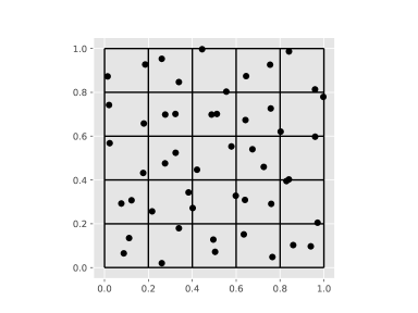
Figure 1: Stratification of $[0,1]^{s}$ when $s=2$ and $k=5$, and two evaluations are performed in each of the $k^{s}=25$ squares. The location of the points are generated as in Haber’s second estimator, which we discuss in Section 2.1.

For $c\in\mathbb{R}^{s}$ and $k\geq 1$, we use the short-hand $B_{k}(c)$ for the hyper-cube $\prod_{i=1}^{s}[c_{i}-1/2k,c_{i}+1/2k]$; in other words, the ball with radius $1/2k$ and centre $r$ with respect to the maximum norm.

For $m\in\mathbb{N}_{0}$ let

$$\mathfrak{C}_{m,k}=\left\{\left(\frac{2j_{1}+1}{2k},\dots,\frac{2j_{s}+1}{2k}\right)\text{ s.t. }\,(j_{1},\dots,j_{s})\in\{-m,\dots,k+m-1\}^{s}\right\}$$ (4)

be the set of the centres of the $(k+2m)^{s}$ hypercubes $B_{k}(c)$ whose union is equal to the set $\mathcal{S}_{m,k}:=[-m/k,1+m/k]^{s}$. In Section 2, we will set $m=0$ and recover the aforementioned stratification; in that case, we will use the short-hand $\mathfrak{C}_{k}:=\mathfrak{C}_{0,k}$. However, in order to define the second (vanishing) estimator in Section 3, we shall take $m\geq 0$.

To each $c\in\mathfrak{C}_{m,k}$ (with $m$, again, fixed and determined by the context), we associate a random variable $U_{c}$ such that

$$U_{c}\sim\mathcal{U}\left(\left[-\frac{1}{2k},\frac{1}{2k}\right]^{s}\right).$$

Notice that the support of $c+U_{c}$ is $B_{k}(c)$.

2 Integration of functions in $\mathcal{C}^{r}\left([0,1]^{s}\right)$

2.1 Preliminaries: Haber’s estimators

In Haber, (1966) Haber introduced the following estimator:

$$\widehat{\mathcal{I}}_{1,k}(f):=\frac{1}{k^{s}}\sum_{c\in\mathfrak{C}_{k}}f(c+U_{c}),\qquad U_{c}\sim\mathcal{U}\left(\left[-\frac{1}{2k},\frac{1}{2k}\right]^{s}\right)$$ (5)

based on $n=k^{s}$ evaluations of $f$, which is optimal for $r=1$; i.e. its RMSE is $\mathcal{O}(n^{-1/2-1/s})$ provided $f\in\mathcal{C}^{1}([0,1]^{s})$. To establish this result, note that each term $f(c+U_{c})$ has expectation $k^{s}\int_{B_{k}(c)}f(u)\mathrm{d}u$ and variance $\mathcal{O}(n^{-2/s})$, since $|f(u)-f(v)|=\mathcal{O}(k^{-1})=\mathcal{O}(n^{-1/s})$ for $u,v\in B_{k}(c)$.

We note in passing that an alternative, and closely related, estimator may be obtained by approximating $f$ with the piecewise constant function $f_{n}$ defined by

$$f_{n}(u)=\sum_{c\in\mathfrak{C}_{k}}f(c)\mathds{1}_{B_{k}(c)}(u),\quad u\in[0,1]^{s}$$

and using that particular $f_{n}$ in (1). Since $\|f-f_{n}\|_{\infty}=\mathcal{O}(n^{-1/s})$ when $f\in\mathcal{C}^{1}([0,1]^{s})$, this alternative estimator is indeed optimal for $r=1$. The estimator defined in (5) is however slightly more convenient to compute, and relies on only $n$ evaluations (versus $2n$ for the alternative estimator).

In Haber, (1967) Haber introduced a second estimator:

$$\widehat{\mathcal{I}}_{2,k}(f):=\frac{1}{k^{s}}\sum_{c\in\mathfrak{C}_{k}}g_{c}(U_{c}),\qquad U_{c}\sim\mathcal{U}\left(\left[-\frac{1}{2k},\frac{1}{2k}\right]^{s}\right)$$ (6)

with $g_{c}(u):=\{f(c+u)+f(c-u)\}/2$ and $n=2k^{s}$, which is optimal for $f\in\mathcal{C}^{2}([0,1]^{s})$. Note that $g_{c}$ is a symmetric function, thus its Taylor expansion at $0$ only includes even order terms:

$$g_{c}(u)=f(c)+\frac{1}{2}u^{T}H_{f}(c)u+\mathcal{O}(k^{-4}),\quad\mbox{for }u\in B_{k}(c)$$ (7)

where $H_{f}(c)$ denotes the Hessian matrix of $f$ at $c$. The term $g_{c}(U_{c})$ has variance $\mathcal{O}(n^{-4/s})$ when $f\in\mathcal{C}^{2}\left([0,1]^{s}\right)$, leading to an $\mathcal{O}(n^{-1/2-2/s})$ RMSE for $\widehat{\mathcal{I}}_{2,k}(f)$.

The estimators introduced in this paper have the same form as Haber’s two estimators; i.e. an average of terms $g_{r,c}(U_{c})$, where $g_{r,c}(U_{c})=f(c)+\mathcal{O}(k^{-r})$ essentially. To achieve this, we consider two approaches: one based on control variates (this section), and another based on combining more than two terms of the form $f(c+\lambda U_{c})$ (Section 3).

2.2 Control variates

One simple way to improve on Haber’s second estimator is to add a control variate based on a Taylor expansion of $g_{c}$. To fix ideas, suppose that $f\in\mathcal{C}^{4}\left([0,1]^{s}\right)$, and add to each term $g_{c}(U_{c})$ in (6) the quantity

$$-\frac{1}{2}U_{c}^{T}H_{f}(c)U_{c}+\mathbb{E}\left[\frac{1}{2}U_{c}^{T}H_{f}(c)U_{c}\right].$$

This does not change the overall expectation, since this extra term has zero mean, and, given (7), it reduces the variance of each term to $\mathcal{O}(n^{-8/s})$.

More generally, for $r\geq 2$, let $p_{c,r-1}$ be the polynomial function that corresponds to the $(r-1)$-order Taylor expansion of $g_{c}$ at $0$, i.e. (2) with $g=g_{c}$ and $u=0$. Then, using (2) and (3), we have

$$|g_{c}(u)-p_{c,r-1}(u)|\leq C\|f\|_{r}\|u\|^{r},\quad\forall u\in[1/2k,1-1/2k]^{s},\quad\forall c\in\mathfrak{C}_{k}$$

for some constant $C<\infty$ (which does not depend on $c$). Letting

$$V_{r,k}(f):=-\frac{1}{k^{s}}\sum_{c\in\mathfrak{C}_{k}}\left\{p_{c,r-1}(U_{c})-\mathbb{E}[p_{c,r-1}(U_{c})]\right\},$$

the variance of the estimator $\mathcal{I}^{*}_{r,k}(f):=\widehat{\mathcal{I}}_{2,k}(f)+V_{r,k}(f)$ is therefore such that

$$\mathrm{Var}\left[\mathcal{I}^{*}_{k}(f)\right] =\frac{1}{k^{2s}}\sum_{c\in\mathfrak{C}_{k}}\mathrm{Var}\left[g_{c}(U_{c})-p_{c,r-1}(U_{c})\right]$$

$$\leq C^{2}\|f\|_{r}^{2}\times k^{-s-2r}$$

$$=C^{\prime}\,\|f\|^{2}_{r}\,n^{-1-2r/s},\qquad C^{\prime}:=C^{2}\times 2^{1+2r/s}.$$

Since $\mathcal{I}^{*}_{k}(f)$ is an unbiased estimator of $\mathcal{I}(f)$, its RMSE is $\mathcal{O}(n^{-1/2-r/s})$. Moreover, with probability one $\mathcal{I}^{*}_{k}(f)=\mathcal{I}(f)$ if $f$ is a polynomial of degree $p<r$ since, in this case, $\|f\|_{r}=0$.

The main drawback of estimator $\mathcal{I}^{*}_{k}(f)$ is that it requires to compute and evaluate derivatives of $f$; that may be feasible in certain cases (using for instance automatic differentiation, see Baydin et al., (2017)). However, it is generally simpler to have an estimator that relies only on evaluations of $f$. Surprisingly, and as shown in the following, higher-order difference methods make it possible to replace, in the definition of $p_{c,r-1}$, the partial derivatives of $f$ by numerical derivatives while preserving the convergence rate of $\mathcal{I}^{*}_{k}(f)$ as well as its ability to integrate exactly polynomials of degree $p<r$.

Higher-order difference methods are widely used in practice for numerical differentiation. However it is surprisingly hard to find a reference providing an explicit definition of an estimate $\hat{D}^{\alpha}f$ of $D^{\alpha}f$ along with an explicit error bound $e_{f}(s,r,|\alpha|)$ for the approximation error $\|\hat{D}^{\alpha}f-D^{\alpha}f\|_{\infty}$. For this reason, in the next subsection we provide two results on numerical differentiation based on higher-order difference methods before coming back to the estimation of $\mathcal{I}(f)$ in the subsequent subsections.

2.3 Numerical differentiation

The result in the following lemma can be used, for $s=1$, to compute an estimate $\hat{D}^{\alpha}f$ of $D^{\alpha}f$ as well as to obtain an upper bound for the approximation error.

Lemma 1.

Let $g\in\mathcal{C}^{l}([0,1])$ for some integer $l\geq 2$, $a\in\{1,\dots,l-1\}$ and $\kappa\in\mathbb{R}^{l}$ be a vector containing $l$ distinct elements. Next, let $e^{(a)}\in\mathbb{R}^{l}$ be such that $e_{a+1}^{(a)}=a!$, $e_{j}^{(a)}=0$ for $j\neq(a+1)$, and let

$$w=A_{\kappa}^{-1}e^{(a)},\quad A_{\kappa}=\begin{pmatrix}1&1&\ldots&1\\ \kappa_{1}&\kappa_{2}&\ldots&\kappa_{l}\\ \vdots&\vdots&\vdots&\vdots\\ \kappa_{1}^{l-1}&\kappa_{2}^{l-1}&\ldots&\kappa_{l}^{l-1}\end{pmatrix}.$$

Let $x\in[0,1]$ and $h>0$ be such that $x+\kappa_{j}h\in(0,1)$ for all $j\in\{1,\dots,l\}$. Then,

$$\left|\frac{\sum_{j=1}^{l}w_{j}g(x+\kappa_{j}h)}{h^{a}}-g^{(a)}(x)\right|\leq h^{l-a}\|g\|_{l}\sum_{j=1}^{l}|w_{j}\kappa_{j}^{l}|.$$

Remark 1.

The matrix $A_{\kappa}$ is invertible since $A_{\kappa}$ is a Vandermonde matrix and $\kappa_{j}\neq\kappa_{l}$ for all $j\neq l$.

Proof.

By construction, $\{w_{j}\}_{j=1}^{l}$ is such that $\sum_{j=1}^{l}w_{j}\kappa^{i}_{j}=0$ for all $i\in\{0,\dots,l-1\}\setminus\{a\}$ and such that $\sum_{j=1}^{l}w_{j}\kappa^{a}_{j}=a!$. Therefore, using (2)-(3), for some $\{\tau_{j}\}_{j=1}^{l}$ in $[-1,1]$ we have

$$\sum_{j=1}^{l}w_{j}g(x+\kappa_{j}h) =\sum_{i=0}^{l-1}h^{i}\frac{g^{(i)}(x)}{i!}\left(\sum_{j=1}^{l}w_{j}\kappa_{j}^{i}\right)+\sum_{j=1}^{l}w_{j}(\kappa_{j}h)^{l}g^{(l)}(x+\tau_{j}\kappa_{j}h)$$

$$=h^{a}g^{(a)}(x)+h^{l}\left(\sum_{j=1}^{l}w_{j}\kappa^{l}_{j}\,g^{(l)}(x+\tau_{j}\kappa_{j}h)\right)$$

and thus

$$\left|g^{(a)}(x)-\frac{\sum_{j=1}^{l}w_{j}g(x+\kappa_{j}h)}{h^{a}}\right| \leq h^{l-a}\left|\sum_{j=1}^{l}w_{j}\kappa_{j}^{l}\,g^{(l)}(x+\tau_{j}\kappa_{j}h)\right|$$

$$\leq h^{l-a}\|g^{(l)}\|_{\infty}\sum_{j=1}^{l}|w_{j}\kappa_{j}^{l}|.$$

The proof is complete. ∎

Remark 2.

Usually, one sets the $\kappa_{j}$’s to small integers; e.g. $\kappa=(0,1,2)$ for $l=3$ and $a=2$ gives the well-known forward formula with first-order accuracy:

$$\frac{g(x)-2g(x+h)+g(x+2h)}{h^{2}}=g^{(2)}(x)+\mathcal{O}(h).$$

If one uses instead so-called central coefficients, e.g. $\kappa=(-1,0,1)$, then one may actually get an extra order of accuracy:

$$\frac{g(x-h)-2g(x)+g(x+h)}{h^{2}}=g^{(2)}(x)+\mathcal{O}(h^{2})$$

as one can check from first principles. We stick to the general case to keep our notations simpler, as it will not have an impact on our general results.

In our case, we need to compute (multivariate) numerical derivatives of $f$ at all the points $c\in\mathfrak{C}_{k}$, simultaneously. The previous lemma indicates that a numerical derivative of $f$ at $c$ is a linear combination of terms of the form $f(c+\kappa_{j}h)$. If we take $h=1/k$, and $\kappa_{j}\in\mathbb{N}$, then $(c+\kappa_{j}h)\in\mathfrak{C}_{k}$ (unless $c+\kappa_{j}\not\in[0,1]^{s}$, which should happen if $c$ is too close to the boundary). This suggests the following strategy: first, compute $f(c)$ for all $c\in\mathfrak{C}_{k}$; then, for a given $\alpha\in\mathbb{N}_{0}^{s}$, approximate $D^{\alpha}f$ at each $c\in\mathfrak{C}_{k}$ by computing appropriate linear combinations of these $f(c)$.

The following lemma formalises this remark. We note in passing that this trick seems to be already known; it is implemented for instance in the package findiff of Baer, (2018) (which we use in our numerical experiments, see Section 5), although it seems rarely mentioned in books on numerical analysis.

Lemma 2.

Let $r\geq 2$. Then, there exist finite constants $\{C_{i,s}\}_{i=1}^{r-1}$ and a finite set $\mathcal{W}_{r}$ of real numbers, which does not depend on $s$, for which the following holds. For $k\geq r$, $c\in\mathfrak{C}_{k}$, $\alpha$ such that $|\alpha|<r$ and $l_{r,\alpha}:=\prod_{i=1}^{|\alpha|_{0}}(r-i+1)$ elements $\{c^{(q)}\}_{q=1}^{l_{r,\alpha}}$ of $\mathfrak{C}_{k}$ such that

1. $\|c-c^{(q)}\|\leq(r-1)/k$ for all $q\in\{1,\dots,l_{s,\alpha}\}$,

2. for all $j\in\{1,\dots,s\}$, if $\alpha_{j}=0$ then $c^{(q)}_{j}=c_{j}$ for all $q\in\{1,\dots,l_{s,\alpha}\}$,

3. for all $j\in\{1,\dots,s\}$, if $\alpha_{j}\neq 0$ then $c_{j}^{(q)}\neq c_{j}^{(q^{\prime})}$ for all $q,q^{\prime}\in\{1,\dots,l_{s,\alpha}\}$ such that $q\neq q^{\prime}$,

there exist real numbers $\{w_{j}\}_{j=1}^{l_{r,\alpha}}$ such that

• each $w_{j}$ is the product of $|\alpha|_{0}$ elements of the set $\mathcal{W}_{r}$,

• the set $\{w_{j}\}_{j=1}^{l_{r,\alpha}}$ depends on $c$ only through the set $\{k(c^{(q)}-c)\}_{q=1}^{l_{r,\alpha}}$, and is therefore independent of $k$,

• for all $f\in\mathcal{C}^{r}([0,1]^{s})$ we have $\big{|}\widehat{D}^{\alpha}_{k}f(c)-D^{\alpha}f(c)\big{|}\leq C_{|\alpha|,s}\,\|f\|_{r}\,k^{-(r-|\alpha|)}$, where

  $$\widehat{D}^{\alpha}_{k}f(c)=k^{|\alpha|}\sum_{j=1}^{l_{r,\alpha}}w_{j}f(c^{(j)}).$$ (8)

For what follows it is important to stress that, in (8), the sets $\{w_{j}\}_{j=1}^{l_{r,\alpha}}$ and $\{c^{(j)}\}_{j=1}^{l_{r,\alpha}}$ are independent of $f$ and that the computational cost of computing these two sets is independent of $k$. We also point out that, building on Lemma 1, the proof of Lemma 2 is constructive and thus can be used in practice to compute a numerical derivative $\widehat{D}^{\alpha}_{k}f(c)$ as defined in (8).

2.4 Proposed estimator

Let $r\geq 3$, $k\geq r$ and $f:[0,1]^{s}\rightarrow\mathbb{R}$. Then, the proposed estimator of $\mathcal{I}(f)$ is

$$\widehat{\mathcal{I}}_{r,k}(f):=\frac{1}{k^{s}}\sum_{c\in\mathfrak{C}_{k}}\Bigg{\{}\frac{f(c+U_{c})+f(c-U_{c})}{2}\\ -\sum_{l=1}^{\lfloor(r-1)/2\rfloor}\sum_{\alpha:\,|\alpha|=2l}\frac{\widehat{D}^{\alpha}_{k}f(c)}{\alpha!}\left(U^{\alpha}_{c}-\prod_{j=1}^{s}d_{k}(\alpha_{j})\right)\Bigg{\}}$$ (9)

where the numerical derivatives $\widehat{D}^{\alpha}_{k}f(c)$’s are as in Lemma 2 and

$$d_{k}(i):=\mathbb{E}[V^{i}]=\begin{cases}\frac{1}{(i+1)(2k)^{i}}&\mbox{if $i$ is even,}\\ 0&\mbox{otherwise,}\end{cases}\qquad\mbox{with }V\sim\mathcal{U}\left(\left[-\frac{1}{2k},\frac{1}{2k}\right]\right).$$

This estimator is based on $n=3k^{s}$ evaluations of $f$: two thirds at random locations, and one third at deterministic locations (the $f(c)$’s for $c\in\mathfrak{C}_{k}$ which are used to compute the derivatives). Note that $\widehat{\mathcal{I}}_{2q,k}(f)=\widehat{\mathcal{I}}_{2q-1,k}(f)$ for all $q\geq 1$, and that only even-order derivatives appear in (9), because of the symmetry of function $g_{c}(u)=\{f(c+u)+f(c-u)\}/2$ (as explained before).

The main drawback of the estimator $\widehat{\mathcal{I}}_{r,k}(f)$ is that its computational cost increases quickly with $r$ and $s$. We may rewrite the second term of (9) as

$$\sum_{c\in\mathfrak{C}_{k}}W_{r,c}f(c)$$

where the $W_{r,c}$’s are random weights that do not depend on $f$. The number of partial derivatives of $f$ of order $|\alpha|$ being equal to $\binom{s+|\alpha|-1}{s-1}$, the number of operations required to compute these weights is:

$$\mathcal{O}\left(sr^{2}k^{s}\sum_{l=1}^{\lfloor(r-1)/2\rfloor}\binom{s+2l-1}{s-1}\right)=\mathcal{O}(r^{s+3}k^{s})$$

which is exponential in $s$.

On the other hand, since the $W_{r,c}$’s are independent of $f$, they may be pre-computed, and re-used for several functions $f$. Alternatively, when $f$ is expensive to compute, the cost of computing these $W_{r,c}$ will remain negligible (relative to the cost of the $n$ evaluations of $f$) whenever $s$ and $r$ are not too high. See Section 5.2 for a practical example where the function of interest $f$ is expensive to compute.

2.5 An alternative estimator

The estimator $\widehat{\mathcal{I}}_{r,k}(f)$ defined in (9) was obtained by adding control variates to Haber’s second estimator (6). By adding similar variates to his first estimator (5), we obtain the following alternative estimator:

$$\begin{split}\widetilde{\mathcal{I}}_{r,k}(f)&:=\frac{1}{k^{s}}\sum_{c\in\mathfrak{C}_{k}}\left(f(c+U_{c})-\sum_{l=1}^{r-1}\sum_{\alpha:\,|\alpha|=l}\frac{\widehat{D}^{\alpha}_{k}f(c)}{\alpha!}\left(U_{c}^{\alpha}-\prod_{j=1}^{s}d_{k}(\alpha_{j})\right)\right)\end{split}$$ (10)

with the derivatives $\widehat{D}^{\alpha}_{k}f(c)$’s as in Lemma 2.

The estimator $\widetilde{\mathcal{I}}_{r,k}(f)$ has the advantage of requiring only $n=2k^{s}$ evaluations of $f$, against $n=3k^{s}$ for $\widehat{\mathcal{I}}_{r,k}(f)$. In addition, $\widetilde{\mathcal{I}}_{r,k}(f)$ has a different expression for each value of $r$, while $\widehat{\mathcal{I}}_{2q,k}(f)=\widehat{\mathcal{I}}_{2q-1,k}(f)$.

On the other hand, computing $\widetilde{\mathcal{I}}_{r,k}(f)$ is more expensive than $\widehat{\mathcal{I}}_{r,k}(f)$, since the former requires to approximate all the partial derivatives of $f$ of order $|\alpha|<r$, while the latter necessitates to compute only those having an even order.

In our numerical experiments, we implement only $\widehat{\mathcal{I}}_{r,k}(f)$. But, for the sake of completeness, we shall state the properties of both estimators in the following section.

2.6 Error bounds

The error bounds presented in this subsection follow directly from the following key lemma, whose proof is in Appendix C.2.

Lemma 3.

Let $f\in\mathcal{C}^{r}([0,1]^{s})$ for some $r\geq 1$. Then there exists, for each $c\in\mathfrak{C}_{k}$ and $k\geq r$, a function $h_{k,c}:[-1/2k,1/2k]^{s}\rightarrow\mathbb{R}$ (which depends implicitly on $r$) such that

$$\widehat{\mathcal{I}}_{r,k}(f)-\mathcal{I}(f)=\frac{1}{k^{s}}\sum_{c\in\mathfrak{C}_{k}}h_{k,c}(U_{c})$$

and such that, for a constant $\widehat{C}_{s,r}<\infty$ independent of $k$ and $f$,

$$\max_{c\in\mathfrak{C}_{k}}\|h_{k,c}\|_{\infty}\leq\widehat{C}_{s,r}\|f\|_{r}k^{-r}.$$

This statement also holds for $\widetilde{\mathcal{I}}_{r,k}(f)$.

The following theorem provides three types of error bounds for the estimators $\widehat{\mathcal{I}}_{r,k}(f)$ and $\widetilde{\mathcal{I}}_{r,k}(f)$, namely an error bound for the RMSE, an error bound that holds with probability one and an error bound that holds with large probability. We recall that the number $n$ of evaluations of $f$ is $n=3k^{s}$ for the former estimator and $n=2k^{s}$ for the latter.

Theorem 1.

Let $f\in\mathcal{C}^{r}([0,1]^{s})$ for some $r\geq 1$ and let $\widehat{C}_{s,r}<\infty$ be as in Lemma 3. Then, for all $k\geq r$,

1. $\mathbb{E}\left[\widehat{\mathcal{I}}_{r,k}(f)\right]=\mathcal{I}(f)$,

2. $\left[\mathbb{E}\big{|}\widehat{\mathcal{I}}_{r,k}(f)-\mathcal{I}(f)\big{|}^{2}\right]^{\frac{1}{2}}\leq\widehat{C}_{s,r}\,\|f\|_{r}\,n^{-\frac{1}{2}-\frac{r}{s}}$,

3. $\mathbb{P}\left(\big{|}\widehat{\mathcal{I}}_{r,k}(f)-\mathcal{I}(f)\big{|}\leq\widehat{C}_{s,r}\,\|f\|_{r}\,n^{-\frac{r}{s}}\right)=1$,

4. For all $\delta\in(0,1)$,

   $$\mathbb{P}\left\{\big{|}\widehat{\mathcal{I}}_{r,k}(f)-\mathcal{I}(f)\big{|}\leq n^{-\frac{1}{2}-\frac{r}{s}}\,\widehat{C}_{s,r}\|f\|_{r}\sqrt{2\log(2/\delta)}\right\}\geq 1-\delta.$$

The results given in 1-4 also hold with $\widehat{\mathcal{I}}_{r,k}(f)$ replaced by $\widetilde{\mathcal{I}}_{r,k}(f)$.

Proof.

We have already mentioned that $\widehat{\mathcal{I}}_{r,k}(f)=\widehat{\mathcal{I}}_{2,k}(f)+\widehat{V}_{r,k}(f)$, where $\widehat{\mathcal{I}}_{2,k}(f)$ is unbiased Haber, (1967) and $\widehat{V}_{r,k}(f)$ has zero mean. (The same remarks apply to $\widetilde{\mathcal{I}}_{k,k}(f)$.) The second and third parts of the theorem are direct consequences of Lemma 3 and the last part of the theorem is a direct consequence of Lemma 3 and of Hoeffding’s inequality. ∎

The second part of the theorem shows that $\widehat{\mathcal{I}}_{r,k}(f)$ and $\widetilde{\mathcal{I}}_{r,k}(f)$ are optimal for integrating a function $f\in\mathcal{C}^{r}([0,1]^{s})$, in the sense that their RMSE converge to zero at the optimal rate (see Section 1). The third part of the theorem states that each realization of the estimators achieves the optimal convergence rate for a deterministic algorithm (again, see Section 1). The last part of the theorem shows that the distribution of $\widehat{\mathcal{I}}_{r,k}(f)$ and of $\widetilde{\mathcal{I}}_{r,k}(f)$ are sub-Gaussian. Finally, and importantly, Theorem 1 shows that for any $k\geq r$ the estimators $\widehat{I}_{r,k}(f)$ and $\widetilde{I}_{r,k}(f)$ are exact if $f$ is a polynomial of degree $p<r$. Indeed, if $f\in\mathcal{C}^{r}([0,1]^{s})$ is a polynomial of degree $p<r$ then $\|f\|_{r}=0$ and thus, by Theorem 1,

$$\mathbb{P}\left(\widehat{\mathcal{I}}_{r,k}(f)=\mathcal{I}(f)\right)=1,\quad\mathbb{P}\left(\widetilde{\mathcal{I}}_{r,k}(f)=\mathcal{I}(f)\right)=1,\quad\forall k\geq r.$$

2.7 Central limit theorem

The following lemma provides a sufficient condition for a central limit theorem to hold for $\widehat{\mathcal{I}}_{r,k}(f)$ and $\widetilde{\mathcal{I}}_{r,k}(f)$.

Lemma 4.

Let $f\in\mathcal{C}^{r}([0,1]^{s})$ for some $r\geq 1$ and assume that there exists a sequence $(v_{k})_{k\geq 1}$ such that $v_{k}\rightarrow\infty$ and such that

$$\mathrm{Var}\left(\widehat{\mathcal{I}}_{r,k}(f)\right)\geq v_{k}k^{-2s-2r},\quad\forall k\geq r.$$

Then,

$$\frac{\widehat{\mathcal{I}}_{r,k}(f)-\mathcal{I}(f)}{\sqrt{\mathrm{Var}\left(\widehat{\mathcal{I}}_{r,k}(f)\right)}}\Rightarrow\mathcal{N}_{1}(0,1).$$

This statement also holds with $\widehat{\mathcal{I}}_{r,k}(f)$ replaced by $\widetilde{\mathcal{I}}_{r,k}(f)$.

Proof of Lemma 4.

We prove only the result for $\widehat{\mathcal{I}}_{r,k}(f)$, the proof for $\widetilde{\mathcal{I}}_{r,k}(f)$ being identical.

Let $k\geq r$ and, for all $c\in\mathfrak{C}_{k}$, let

$$X_{k,c}=\frac{1}{k^{s}}\,h_{k,c}(U_{c})$$

with $h_{k,c}(U_{c})$ as in Lemma 3. Note that $\widehat{\mathcal{I}}_{r,k}(f)-\mathcal{I}(f)=\sum_{c\in\mathfrak{C}_{k}}X_{k,c}$ and that $\{X_{k,c}\}_{c\in\mathfrak{C}_{k}}$ is a set independent random variables for all $k\geq r$. Then, by Lindeberg-Feller central limit theorem (see Billingsley, (1995), Theorem 27.2, page 359) to prove the lemma it is enough to show that, as $k\rightarrow\infty$,

$$\frac{1}{B_{k}^{2}}\sum_{c\in\mathfrak{C}_{k}}\mathbb{E}\left[X_{k,c}^{2}\mathds{1}(X_{k,c}^{2}>\epsilon B_{k}^{2})\right]\rightarrow 0,\quad\forall\epsilon>0$$ (11)

where $B_{k}=\mathrm{Var}\left(\widehat{\mathcal{I}}_{r,k}(f)\right)^{1/2}$ for all $k$.

To show (11) remark first that, by Theorem 1 and under the assumptions of the lemma, we have

$$v_{k}k^{-2s-2r}\leq B_{k}^{2}\leq C_{f,r,s}k^{-s-2r}$$ (12)

where $C_{f,r,s}=\widehat{C}^{2}_{s,r}\|f\|^{2}_{r}$ with $\widehat{C}_{s,r}<\infty$ as in Theorem 1.

Next, let $k\geq r$ and $c\in\mathfrak{C}_{k}$, and note that, by Lemma 3,

$$X_{k,c}^{2}=k^{-2s}\,h_{k,c}(U_{c})^{2}\leq C_{f,s,r}k^{-2s-2r},\quad\mathbb{P}-a.s.$$

which, together with (12), implies that for all $\epsilon>0$ and $\mathbb{P}$-a.s.  we have

$$\mathds{1}(X_{k,c}^{2}>\epsilon B_{k}^{2}) \leq\mathds{1}\left(C_{f,s,r}k^{-2s-2r}>\epsilon B_{k}^{2}\right)$$

$$\leq\mathds{1}\left(C_{f,s,r}k^{-2s-2r}>\epsilon v_{k}k^{-2s-2r}\right)$$

$$=\mathds{1}\left(C_{f,s,r}>\epsilon v_{k}\right).$$

Since $v_{k}\rightarrow\infty$, (11) follows and the proof is complete. ∎

By Lemma 4, a CLT therefore holds for $\widehat{\mathcal{I}}_{r,k}(f)$ and $\widetilde{\mathcal{I}}_{r,k}(f)$ if the variance of these estimators does not converge to zero too quickly as $k\rightarrow\infty$. Noting that the lower bound on the variances assumed in Lemma 4 converges to zero much faster than the upper bound given in Theorem 1 (part 2), we conjecture that a CLT holds in general for $\widehat{\mathcal{I}}_{r,k}(f)$ (and $\widetilde{\mathcal{I}}_{r,k}(f)$).

We are able to establish this conjecture provided that the numerical derivatives are computed in the following way. We introduce $p_{r,k}:=\lceil k/r\rceil^{s}$ hyper-cubes $\tilde{B}_{q}$ of volume $(r/k)^{s}$, $q=1,\ldots,p_{r,k}$, such that $\cup_{q=1}^{p_{r,k}}\tilde{B}_{q}=[0,1]^{s}$, and let $\tilde{B}_{q}=\cup_{j=1}^{r^{s}}B_{k}(c_{j}^{q})$ with $\{c_{j}^{q}\}_{q=1}^{p_{r,k}}\subset\mathfrak{C}_{k}$ such that the $B_{k}(c_{j}^{q})$’s are contiguous. Then, to each $c\in\mathfrak{C}_{k}$ we assign a $q(c)$ such that $c\in B_{q(c)}$ and impose that the numerical derivatives at $c$ are computed using only points $c^{\prime}\in B_{q(c)}$. The following lemma establishes that this way of computing numerical derivatives ensures that the condition in Lemma 4 is fulfilled.

Lemma 5.

Let $f\in\mathcal{C}^{r}([0,1]^{s})$ for some $r\geq 2$ and, for all $k\geq r$, $\alpha$ such that $|\alpha|<r$ and $c\in\mathfrak{C}_{k}$, let $\widehat{D}^{\alpha}_{k}f(c)$ be as defined in Lemma 2 with $c_{j}\in B_{q(c)}$ for all $j\in\{1,\dots,l_{r,\alpha}\}$. In addition, for all $\alpha$ such that $|\alpha|=r$ let $g_{\alpha}:[0,1]^{s}\rightarrow\mathbb{R}$ be defined by $g_{\alpha}(u)=(-1/2+u)^{\alpha}$, $u\in[0,1]^{s}$, and let

$$\widehat{\sigma}^{2}_{f,r}=r^{2r+s}\sum_{|\alpha|=r}\sum_{|\alpha^{\prime}|=r}\frac{\mathrm{Cov}\left(\,\widehat{\mathcal{I}}_{r,r}(g_{\alpha}),\widehat{\mathcal{I}}_{r,r}(g_{\alpha^{\prime}}\,)\right)}{\alpha!\alpha^{\prime}!}\int_{[0,1]^{s}}D^{\alpha}f(u)\,D^{\alpha^{\prime}}f(u)\mathrm{d}u.$$ (13)

Then

$$\lim_{k\rightarrow\infty}\left\{k^{s+2r}\mathrm{Var}\left(\widehat{\mathcal{I}}_{r,k}(f)\right)\right\}=\widehat{\sigma}^{2}_{f,r}.$$ (14)

The same result holds if $\widehat{\mathcal{I}}_{r,k}(f)$ is replaced by $\widetilde{\mathcal{I}}_{r,k}(f)$.

To understand why the numerical derivatives assumed in Lemma 5 are convenient to show that (14) holds, let $[a,b]\subset[0,1]^{s}$ and $f_{[a,b]}:[0,1]^{s}\rightarrow\mathbb{R}$ be defined by

$$f_{[a,b]}(u)=f(a+u(b-a)),\quad u\in[0,1]^{s}$$

where, for all $u$, the product $u(b-a)$ must be understood as being component-wise. In addition, assume that $k=mr$ for some integer $m\geq 1$, so that the set $[0,1]^{s}$ can be covered by $m^{s}$ hypercubes $\{\tilde{B}_{q}\}_{q=1}^{m^{s}}$ of volume $m^{-s}$. Then, under the assumptions on the $\widehat{D}^{\alpha}_{k}f(c)$’s made in Lemma 5,

$$\widehat{\mathcal{I}}_{r,mr}(f)\stackrel{{\scriptstyle\mathclap{\mbox{\tiny{dist}}}}}{{=}}\sum_{q=1}^{m^{s}}\widehat{\mathcal{I}}_{r,mr}(f\mathds{1}_{\tilde{B}_{q}})\stackrel{{\scriptstyle\mathclap{\mbox{\tiny{dist}}}}}{{=}}\frac{1}{m^{s}}\sum_{q=1}^{m^{s}}\widehat{\mathcal{I}}_{r,r}(f_{\tilde{B}_{q}})$$

where the terms of the sum are independent random variables. Since $\widehat{\mathcal{I}}_{r,r}$ is a stochastic quadrature of degree $r-1$, it follows from (Haber,, 1969, Theorem 2) that

$$\lim_{m\rightarrow\infty}\mathrm{Var}\left\{(mr)^{s/2+r}\widehat{\mathcal{I}}_{r,mr}(f)\right\}=\widehat{\sigma}^{2}_{f,r}.$$

Lemma 5 extends this result to the case where $k$ is not a multiple of $r$.

Combining Lemma 4 and Lemma 5 we readily obtain the following result.

Theorem 2.

Let $f\in\mathcal{C}^{r}([0,1]^{s})$ for some $r\geq 2$ and assume that, for all $k\geq r$, $c\in\mathfrak{C}_{k}$ and $\alpha$ such that $|\alpha|<r$, the numerical derivative $\widehat{D}^{\alpha}_{k}f(c)$ and the constant $\widehat{\sigma}^{2}_{f,r}$ are as defined in Lemma 5. Then, if $\widehat{\sigma}^{2}_{f,r}>0$ we have

$$\frac{\widehat{\mathcal{I}}_{r,k}(f)-\mathcal{I}(f)}{\sqrt{\mathrm{Var}\left(\widehat{\mathcal{I}}_{r,k}(f)\right)}}\Rightarrow\mathcal{N}_{1}(0,1).$$

This statement also holds if $\widehat{\mathcal{I}}_{r,k}(f)$ is replaced by $\widetilde{\mathcal{I}}_{r,k}(f)$.

3 Integration of vanishing functions

3.1 Principle

We now focus on functions whose derivatives are null at the boundary of the set $[0,1]^{s}$. Formally, for $r\geq 1$ we let

$$\mathcal{C}^{r}_{0}\left([0,1]^{s}\right):=\left\{f\in\mathcal{C}^{r}([0,1]^{s})\text{ s.t. }\max_{\alpha:|\alpha|\leq r}\left|D^{\alpha}f(u)\right|=0\text{ or all }u\in\partial[0,1]^{s}\right\}$$

and consider the problem of approximating $\mathcal{I}(f)$ for $f\in\mathcal{C}^{r}_{0}([0,1]^{s})$. Our objective is to derive an estimator that has the same optimality properties as the estimator introduced in the previous section, while being cheaper to compute when $f\in\mathcal{C}^{r}_{0}\left([0,1]^{s}\right)$. Vanishing functions may arise for instance when performing importance sampling with a heavy-tail proposal distribution; see the second set of numerical experiments (Section 5.2) for an illustration of this idea, and see Appendix A for a longer discussion of the practical relevance of vanishing functions.

We return to Haber’s second estimator:

$$\widehat{\mathcal{I}}_{2,k}(f)=\frac{1}{k^{s}}\sum_{c\in\mathfrak{C}_{k}}g_{c}(U_{c}),\quad U_{c}\sim\mathcal{U}\left(\left[-\frac{1}{2k},\frac{1}{2k}\right]^{s}\right)$$

where, assuming $f\in\mathcal{C}^{4}\left([0,1]^{s}\right)$,

$$g_{c}(u) =\frac{f(c+u)+f(c-u)}{2}=f(c)+\frac{1}{2}u^{T}H_{f}(c)u+\mathcal{O}(\|u\|^{4}),$$

and $H_{f}(c)$ is the Hessian of $f$ at $c$. To get a smaller error, one may combine more than two terms; e.g. with four terms:

$$\frac{g_{c}(\lambda u)-\lambda^{2}g_{c}(u)}{1-\lambda^{2}} =\frac{f(c+\lambda u)+f(c-\lambda u)-\lambda^{2}f(c+u)-\lambda^{2}f(c-u)}{2(1-\lambda^{2})}$$

$$=f(c)+\mathcal{O}(\|u\|^{4}).$$

The resulting estimator will then be a linear combination of averages of the form $k^{-s}\sum_{c}f(c+\lambda U_{c})$, for a given $\lambda$. But, if $|\lambda|\neq 1$, such an average will typically not have the desired expectation $\mathcal{I}(f)$, since the support of $c+\lambda U_{c}$ is a hyper-cube inflated by a factor $\lambda$.

To address this issue, we note first that, since $f\in\mathcal{C}^{r}_{0}\left([0,1]^{s}\right)$, we may extend $f$ to $\bar{f}\in\mathcal{C}^{r}(\mathbb{R}^{s})$, with $\bar{f}(u)=f(u)$ if $u\in[0,1]^{s}$, and $\bar{f}(u)=0$ otherwise. This implies that:

$$\mathcal{I}(f)=\int_{[0,1]^{s}}f(u)\mathrm{d}u=\int_{\mathbb{R}^{s}}\bar{f}(u)\mathrm{d}u=\sum_{c\in\mathfrak{C}_{\infty,k}}\int_{B_{k}(c)}\bar{f}(u)\mathrm{d}u$$

where $\mathfrak{C}_{\infty,k}$ is simply (4) with $m=+\infty$; i.e. the (infinite) set of centres of hypercubes of volume $k^{-s}$, the union of which is $\mathbb{R}^{s}$.

Second, if we restrict $\lambda$ to values such that $|\lambda|=1,3,5,\ldots$, we observe that the support of $(c+\lambda U_{c})$ is the union of $|\lambda|^{s}$ contiguous hyper-cubes in $\mathfrak{C}_{\infty,k}$. If we sum over $c\in\mathfrak{C}_{\infty,k}$, we make sure that each hyper-cube is ‘visited’ the same number of times. In practice, we need to consider only $c$ such that support of $(c+\lambda U_{c})$ intersects with $[0,1]^{s}$, since the corresponding integral is zero otherwise. The following lemma formalises these ideas.

Lemma 6.

Let $g\in L_{1}([0,1]^{s})$, $\lambda\in\{\pm(2i+1),\,i\in\mathbb{N}_{0}\}$, $k\geq 2$, and $\bar{g}:\mathbb{R}^{s}\rightarrow\mathbb{R}$ be such that $\bar{g}(u)=g(u)$ if $u\in[0,1]^{s}$ and $\bar{g}(u)=0$ otherwise. Then,

$$\mathbb{E}\left[\frac{1}{k^{s}}\sum_{c\in\mathfrak{C}_{m,k}}\bar{g}(c+\lambda U_{c})\right]=\int_{[0,1]^{s}}g(u)\mathrm{d}u,\quad\forall m\geq(|\lambda|-1)/2.$$

3.2 Proposed estimator

We are now able to define our vanishing estimator. Assume $r\geq 1$ is fixed, and $f\in\mathcal{C}^{r}_{0}\left([0,1]^{s}\right)$. Let $(\lambda_{j})_{j=1}^{\infty}$ be the sequence $1,-1,3,-3,5,-5,\ldots$, and

$$m_{r}:=\max\{|\lambda_{j}|\}_{j=1}^{r}=\begin{cases}r,&\text{ if $r$ is odd}\\ r-1,&\text{ otherwise}\end{cases}$$

$$\gamma^{(r)}:=\Gamma^{-1}_{r}\begin{pmatrix}1\\ 0\\ \vdots\\ 0\end{pmatrix},\quad\Gamma_{r}:=\begin{pmatrix}1&1&\ldots&1\\ \lambda_{1}&\lambda_{2}&\ldots&\lambda_{r}\\ \vdots&\vdots&\vdots&\vdots\\ \lambda_{1}^{r-1}&\lambda_{2}^{r-1}&\ldots&\lambda_{r}^{r-1}\end{pmatrix}.$$

The matrix $\Gamma_{r}$ is a Vandermonde matrix and thus, since $\lambda_{j}\neq\lambda_{l}$ for all $j\neq l$, this matrix is invertible. In addition, using Taylor’s theorem it is easy to check that $\gamma^{(r)}$ is the vector of coefficients such that

$$g_{r,c}(u):=\sum_{j=1}^{r}\gamma_{j}^{(r)}\bar{f}(c+\lambda_{j}u)=f(c)+\mathcal{O}(\|u\|^{r}).$$ (15)

We now define our vanishing estimator as follows:

$$\widehat{\mathcal{I}}^{0}_{r,k}(f):=\frac{1}{k^{s}}\sum_{c\in\mathfrak{C}_{m_{r},k}}g_{r,c}(U_{c}),\qquad U_{c}\sim\mathcal{U}\left(\left[-\frac{1}{2k},\frac{1}{2k}\right]^{s}\right).$$ (16)

When $r=1$ or $r=2$, we recover Haber’s estimators: $\widehat{\mathcal{I}}^{0}_{r,k}(f)=\widehat{\mathcal{I}}_{r,k}(f)$ for $r=1,2$. $\widehat{\mathcal{I}}^{0}_{r,k}(f)$ is clearly cheaper (and simpler) to compute than the general estimator $\widehat{\mathcal{I}}_{r,k}(f)$ of the previous section, as the latter required computing a $\mathcal{O}(e^{s})$ number of numerical derivatives. The unbiasedness of $\widehat{\mathcal{I}}^{0}_{r,k}(f)$ is a direct consequence of Lemma 6. From (15), we see that the variance of $\widehat{\mathcal{I}}^{0}_{r,k}(f)$ is $\mathcal{O}(n^{-1-2r/s})$. It has therefore the same RMSE rate as the estimator considered in Section 2. These and other properties are stated in Theorem 3 below.

Before that, we must clarify what we mean by $n$ in this context. We may define $n$ to be the number of evaluations of $\bar{f}$; in this case, $n=r(k+2m_{r})^{s}$, since $|\mathfrak{C}_{m_{r},k}|=(k+2m_{r})^{s}$. Or we may define it to be the number of evaluations of $f(u)$ for $u\in[0,1]^{s}$. In that case, $n$ is random, with expectation $rk^{s}$. (To see this, apply Lemma 6 to function $g(u)=1$.) It is also bounded, i.e. $(k-2m_{r})^{s}\leq n\leq(k+2m_{r})^{s}$ with probability one. Hence, whatever the chosen definition of $n$, the statement $k=\mathcal{O}(n^{-1/s})$ remains correct.

Theorem 3.

Let $f\in\mathcal{C}_{0}^{r}([0,1]^{s})$ for some $r\geq 1$. Then, for all $k\geq 2$ we have $\mathbb{E}[\widehat{\mathcal{I}}^{\,0}_{r,k}(f)]=\mathcal{I}(f)$ and there exists a constant $\widehat{C}^{\,0}_{f,s,r}<\infty$ such that

$$\mathbb{E}\big{[}|\widehat{\mathcal{I}}^{\,0}_{r,k}(f)-\mathcal{I}(f)|^{2}\big{]}^{1/2}\leq\widehat{C}^{\,0}_{f,s,r}n^{-\frac{1}{2}-\frac{r}{s}},\quad\mathbb{P}\left(|\widehat{\mathcal{I}}^{\,0}_{r,k}(f)-\mathcal{I}(f)|\leq\widehat{C}^{\,0}_{f,s,r}n^{-\frac{r}{s}}\right)=1$$

and such that, for all $\delta\in(0,1)$,

$$\mathbb{P}\left\{|\widehat{\mathcal{I}}^{\,0}_{r,k}(f)-\mathcal{I}(f)|\leq n^{-\frac{1}{2}-\frac{r}{s}}\,\widehat{C}^{\,0}_{f,s,r}\sqrt{2\log\left(2/\delta\right)}\right\}\geq 1-\delta.$$

Proof.

As in Lemma 3: for $k\geq 2$ and $c\in\mathfrak{C}_{m_{r},k}$, let $h_{k,c}:[0,1]^{s}\rightarrow\mathbb{R}$ be defined by

$$h_{k,c}(u):=g_{r,c}(u)-\mathbb{E}[g_{r,c}(U_{c})],\quad u\in[0,1]^{s}$$

so that $\widehat{\mathcal{I}}_{r,k}(f)-\mathcal{I}(f)=k^{-s}\sum_{c\in\mathfrak{C}_{m_{r},k}}h_{r,c}(U_{c})$. (Function $h_{k,c}$ also depends on $r$ implicitly.)

Let $u\in[-1/2k,1/2k]^{s}$ and note that, from (15) and the definition of $g_{r,c}$:

$$\begin{split}|h_{k,c}(u)|&\leq\|f\|_{r}\sum_{j=1}^{r}|\gamma^{(r)}_{j}\lambda_{j}^{r}|\sum_{\alpha:|\alpha|=r}\frac{\big{|}u^{\alpha}+\prod_{j:\alpha_{j}\neq 0}d_{k}(j)\big{|}}{\alpha!}\\ &\leq\Big{(}\|f\|_{r}\sum_{j=1}^{r}|\gamma^{(r)}_{j}\lambda_{j}^{r}|\Big{)}\left(2^{-r}k^{-r}+k^{-r}\right)\end{split}$$ (17)

where the second inequality uses the fact that $d_{k}(j)\leq k^{-j}$ for all $j\in\mathbb{N}$.

By (17) there exists a constant $C<\infty$ such that,

$$|h_{k,c}(u)|\leq Ck^{-r},\quad\forall u\in[-1/2k,1/2k]^{s},\quad\forall c\in\mathfrak{C}_{m_{r},k},\quad\forall k\geq 2$$

and thus, since by Lemma 6 the estimator $\widehat{\mathcal{I}}^{\,0}_{r,k}(f)$ is unbiased, the proof of theorem follows from the same remarks as in the proof of Theorem 1. ∎

4 Practical details

4.1 Variance estimation

One advantage of the standard Monte Carlo estimator is that it is possible to estimate its variance from a single run. It does not seem possible to do so with the estimators proposed in this paper. However, we highlight briefly a method to approximate the variance from a potentially small number $l\geq 2$ of independent runs. This method is actually a generalisation of an approach outlined in Section 5 of Haber, (1966) for the estimator (5).

Consider a generic estimator of the form:

$$\widehat{\mathcal{I}}=\frac{1}{n}\sum_{i=1}^{n}Y_{i}$$

where the $Y_{i}$’s are independent but not (necessarily) identically distributed. Both estimators presented in this paper are of this form (up to some notation adjustment); e.g. for the vanishing estimator, $Y_{i}$ may be identified with $g_{r,c}(U_{c})$, see (16).

Assume we obtain $l\geq 2$ realisations of the estimator $\widehat{\mathcal{I}}$, based on independent copies $Y_{n}^{(j)}$ of the $Y_{n}$. Since

$$\mathrm{Var}(\widehat{\mathcal{I}})=\frac{1}{n^{2}}\sum_{i=1}^{n}\mathrm{Var}(Y_{i})$$

take, as an estimator of $\mathrm{Var}(\widehat{\mathcal{I}})$,

$$\hat{V}:=\frac{1}{n^{2}}\sum_{i=1}^{n}\frac{1}{l-1}\sum_{j=1}^{l}(Y_{i}^{(j)}-\bar{Y}_{i})^{2},\qquad\bar{Y}_{i}:=\frac{1}{l}\sum_{j=1}^{l}Y_{i}^{(j)}.$$

It is easy to establish that, for the two types of estimators introduced in this paper, $\widehat{\mathcal{I}}_{r,k}(f)$ and $\widehat{\mathcal{I}}^{0}_{r,k}(f)$ (for a given $r\geq 1$), one has, for a fixed $l\geq 1$:

$$\mathrm{Var}(\hat{V})=\mathcal{O}(n^{-3-4r/s})$$

which is $n^{-1}$ smaller than the square of $\mathcal{O}(n^{-1-2r/s})$, the rate at which the true variance goes to zero.

In other words, estimator $\hat{V}$ will have a small relative error as soon as $n$ is large (even for a small $l$). Of course, if we generate $l$ independent realisations of a given estimator (preferably in parallel), then we should return as a final estimate the average of these $l$ realisations, together with an estimate of its variance, that is, $\hat{V}/l$.

4.2 Automatic order selection for the vanishing estimator

Given (15) and (16), we may rewrite the vanishing estimator as follows:

$$\widehat{\mathcal{I}}^{0}_{r,k}(f)=\sum_{j=1}^{r}\gamma_{j}^{(r)}\left\{\frac{1}{k^{s}}\sum_{c\in\mathfrak{C}_{m_{r},k}}\bar{f}(c+\lambda_{j}U_{c})\right\}=\sum_{j=1}^{r}\gamma_{j}^{(r)}\left\{\frac{1}{k^{s}}\sum_{c\in\mathfrak{C}_{m_{j},k}}\bar{f}(c+\lambda_{j}U_{c})\right\}$$

where in the second line we use the fact that $\bar{f}(c+\lambda_{j}U_{c})=0$ whenever $c\notin\mathfrak{C}_{m_{j},k}$.

We may pre-compute the $r$ averages above, and use them to compute simultaneously $\widehat{\mathcal{I}}^{0}_{r^{\prime},k}(f)$ for $r^{\prime}=1,\ldots,r$, at (essentially) the same cost as computing only $\widehat{\mathcal{I}}^{0}_{r,k}(f)$. If we generate several copies of these estimators, we may then choose the value $r^{\prime}$ with the smallest estimated variance (using the variance estimator proposed in the previous section). We may use a similar approach for the non-vanishing estimator $\widehat{\mathcal{I}}_{r,k}(f)$, but in that case there does not seem to be any short-cut for computing simultaneously $\widehat{\mathcal{I}}_{r,k}(f)$ for different values of $r$.

5 Numerical experiments

In this section, we assess and compare estimators of expectations $\mathcal{I}(f)$ as follows. For a fixed function $f:[0,1]^{s}\rightarrow\mathbb{R}$ and a range of values for $k$, we generate 50 independent copies of the considered estimators, and produce plots where:

• the $x-$axis is the number of evaluations of $f$. When this quantity is random (vanishing estimator), we report the average over the independent runs.

• the $y-$axis is a measure of the relative error; that is, either the mean squared error (MSE) divided by the true value of $\mathcal{I}(f)$, when this quantity is known, or the empirical variance divided by the square of the average, when it is not. In the former (resp. latter) case, the label of the $y-$axis is rel-mse (resp. rel-var). In both cases, we discard results where the relative error is too close to machine epsilon (i.e. when MSE or variance is not $\gg 10^{-32}$ ). In such cases, the corresponding estimates may be considered as exact (up to machine epsilon).

It is customary in this type of plot to overlay a straight line that corresponds to the expected rate, i.e. $\mathcal{O}(n^{-1+2r/d})$ for our estimators. (The log-scale is used on both axes.) However, in our case, the performance of our estimators (often) matches closely these rates, making these lines hard to distinguish. For this reason we do not plot them in what follows.

An open-source python package implementing the two proposed estimators and the following numerical experiments may be found at https://github.com/nchopin/cubic_strat. The numerical derivatives that appear in the control variates of the non-vanishing estimator were computed by the the findiff package of Baer, (2018). We note that the numerical derivatives computed with this package are not implemented in a way which ensures that we have a CLT for $\widehat{\mathcal{I}}_{r,k}(f)$ (that is, they do not verify the assumptions of Theorem 2).

5.1 Comparison between the non-vanishing estimator and Dick’s estimator

As mentioned in the introduction, in Dick, (2011) Dick introduced higher-order estimators of $\mathcal{I}(f)$ (henceforth, Dick’s estimators), based on scrambled digital nets, which achieve $\mathcal{O}(n^{-1/2-\alpha+\epsilon})$ RMSE for functions $f\in\mathcal{D}^{\alpha}([0,1]^{s})$, $\alpha\geq 2$, the set of functions such that all partial derivatives obtained by differentiating with respect to each variable up to $\alpha$-times is square integrable. When $s\geq 2$, this estimator does not require the existence of the same number of partial derivatives as our stratified estimators (even if we set $r=s\times\alpha$). For instance, for $s=2$, denoting $u=(x,y)$, Dick’s estimator requires the existence of $\partial f/\partial x$, $\partial f/\partial y$ and $\partial^{2}f/\partial x\partial y$ at order $\alpha=1$, while our stratified estimator requires only the first two when $r=1$; or, alternatively, these three derivatives plus $\partial^{2}f/\partial x^{2}$, $\partial^{2}f/\partial y^{2}$ at order $r=2$. This technical point should be kept in mind in the following comparison, where Dick’s estimator is implemented using the Sobol’ sequence as underlying digital sequence.

We consider the following functions: for $s=1$, $f_{1}(u)=ue^{u}$, and for $s\geq 2$,

$$f(u)=\left(\prod_{j=1}^{s}u_{j}^{j-1}\right)\exp\left(\prod_{j=1}^{s}u_{j}\right).$$

Note that $\mathcal{I}(f_{1})=1$, and $\mathcal{I}(f_{s})=e-\sum_{j=0}^{s-1}(1/j!)$ for $s\geq 2$. The aforementioned paper used the first two functions of this sequence to illustrate the numerical performance of Dick’s estimators. We compare the performance of Dick’s higher-order estimators (for $\alpha=1,2,3,4$) with our non-vanishing estimator (for $r=1,2,4,6,8$, and, in addition, $r=10$ for $s=1$ and $s=2$); see Figures 2 and 3.

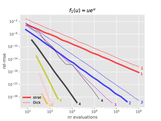
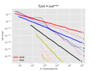
Figure 2: Relative MSE (mean squared error) vs number of evaluations for the vanishing estimator (thick lines) and Dick’s estimator (dotted line). The value of $r$ (stratified) or $\alpha$ (Dick’s) are printed next to each curve. Left: $f_{1}$; Right: $f_{2}$.

For $s=1$ (left panel of Figure 2), both estimators require exactly the same number of derivatives, hence the comparison is straightforward. Both estimators show the expected MSE rate, $\mathcal{O}(n^{-1+2r})$, (taking $\alpha=r$); on the other hand, the stratified estimator seems to consistently have lower MSE.

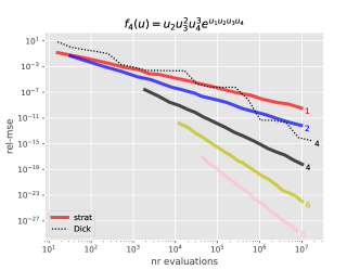
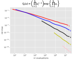
Figure 3: Same plot as in Figure 2 for functions $f_{4}$ (left) and $f_{6}$ (right).

For $s=2$ (right panel of Figure 2), the comparison becomes less straightforward, as we explained above. The fact that Dick’s estimator shows intermediate performance between the stratified estimators for $r=1$ and $r=2$ is reasonable, since it requires strictly more partial derivatives than for $r=1$, and strictly less than for $r=2$; as discussed in the example above. On the other hand, Dick’s estimator at order $\alpha=4$ seems outperformed by both the same estimator at orders $\alpha=2$ and 3, and the stratified estimator at order $r=4$. This is despite the fact that Dick’s estimator with $\alpha=4$ requires strictly more partial derivatives than the stratified estimator with $r=4$. This suggests that, when $\alpha$ increases, Dick’s estimator requires a larger and larger number of evaluations before exhibiting the expected rate of convergence.

For $s=4$ (left panel of Figure 3), we plot only the relative MSE of Dick’s estimator for $\alpha=4$. Again, we observe the same phenomenon: i.e. even with $10^{7}$ evaluations it is not yet competitive with the stratified estimator (with $r=4$) despite requiring more partial derivatives.

In all these plots, the MSE of the proposed estimator matches very closely the expected rate. On the other hand, recall that, for $r\geq 4$, the estimator requires $3k^{s}$ evaluations of $f$, and is properly defined only for $k\geq r$. (In addition, the way the numerical derivatives are computed in package findiff imposes that $k\geq 3r/2-1$.) This implies that this estimator is only defined for a large number of evaluations when $r$ and $s$ are large, as shown in Figures 2 and 3. This is of course a limitation of the non-vanishing estimator. We shall see that the vanishing estimator is less affected by this issue; i.e. it may be computed for smaller values of $n$.

5.2 Vanishing estimator: Bayesian model choice

We now consider a class of vanishing functions in order to assess our vanishing estimator. We construct these functions so that their integral equals the marginal likelihood $\int p(\beta)L(y|\beta)\mathrm{d}\beta$ of a Bayesian statistical model, where $\beta\in\mathbb{R}^{s}$, $p(\beta)$ is a Gaussian prior density (with mean 0, and covariance $5^{2}I_{s}$), $L(y|\beta)$ is the likelihood of a logistic regression model: $L(y|\beta)=\prod_{i=1}^{n}F(y_{i}\beta^{T}x_{i})$, $F(z)=1/(1+e^{-z})$, and the data $(x_{i},y_{i})_{i=1}^{n}$ consist of predictors $x_{i}\in\mathbb{R}^{s}$ and labels $y_{i}\in\{-1,1\}$.

We adapt the importance sampling approach described in Chopin and Ridgway, (2017) to approximate such quantities as follows: we obtain numerically the mode $\hat{\beta}$, and the Hessian at $\beta=\hat{\beta}$, of the function $h(\beta)=\log\{p(\beta)L(y|\beta)\}$; hence $h(\beta)\approx h(\hat{\beta})-(1/2)(\beta-\hat{\beta})^{T}H(\beta-\hat{\beta})$. Then we set $f(u)=\exp\{h(\hat{\beta}+L\psi_{s}(u))\}$, with $L$ the Cholesky lower triangle of $H$, $LL^{\top}=H$, and $\psi_{s}$ the function defined in Appendix A (for $\tau=1.5$), which maps $(0,1)^{s}$ into $\mathbb{R}^{s}$.

As in Chopin and Ridgway, (2017), we consider the Pima dataset (which has 10 predictors, if we include an intercept). More precisely, for $s=2$, 4, 6, and 8, we take the first $s$ predictors, and compute the corresponding marginal likelihoods. Note that computing these quantities for all possible subsets of the predictors is a standard way to perform variable selection in Bayesian inference.

Figure 4 showcases the performance of the vanishing estimators for $s=2$ to 8 and at orders 1 to 10 (for $s=2$ and $s=4$), 8 (for $s=6$), and 4 (for $s=8$). Results for higher orders are not displayed for $s=6$ and $s=8$ because they did not lead to lower variance even for the highest values of number of evaluations.

Note the slightly different behaviour relative to the previous example. The vanishing estimator is defined for lower numbers of evaluations. On the other hand, it exhibits the expected rate only for a large enough number of evaluations. As expected, the relative gain obtained by increasing $r$ decreases with the dimension (and requires a larger and larger number of evaluations to appear clearly).

Notice that, in Figure 4, the number of evaluations has a different range for different values of $r$. This is because the number of evaluations at order $r$ is $rk^{s}$, and we considered the same range of values for $k$. It was convenient to do so, because, as explained in Section 4.2, it is possible to compute simultaneously the vanishing estimators at orders 1 to, say $r_{\max}$ (using the same random numbers), at the cost of obtaining the estimator at highest order, $r_{\max}$.

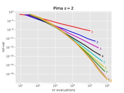
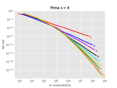
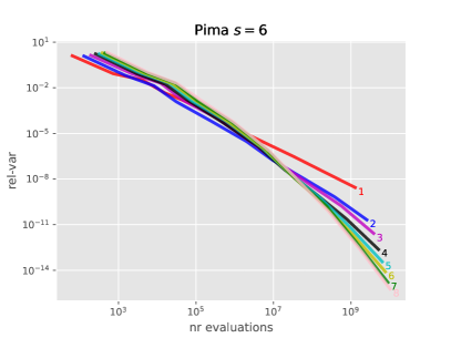
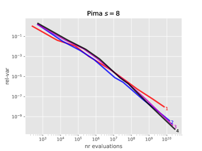
Figure 4: Relative variance of the vanishing estimator versus number of evaluations for Pima example, with $s=2$, 4, 6, 8.

See Appendix B for a comparison of the non-vanishing and vanishing estimators on this example.

6 Future work

The main limitation of cubic stratification is that it cannot realistically work for $s\gg 10$, since the number of cubes required to partition $[0,1]^{s}$ is $k^{s}$. We could use rectangles instead, and take $n=\prod_{i=1}^{s}k_{i}$, with $k_{i}$ smaller (or even $=1$) when $f$ is nearly constant in component $i$, a bit in the spirit of Sloan and Woźniakowski, (1998). Determining how we could choose the $k_{i}$ in a meaningful way is left for future work.

Appendix A Relevance of vanishing functions

Consider the problem of approximating the integral of a function $g$ over $\mathbb{R}^{s}$. A common strategy is to rewrite this integral as an expectation with respect to a chosen, $[0,1]^{s}$-supported distribution; and then use Monte Carlo to approximate it. Since $\lim_{\|x\|\rightarrow\infty}g(x)=0$, this expectation will often be an integral of a vanishing function. Thus, one may use instead our vanishing estimator to approximate the integral of interest.

The following lemma outlines a particular recipe to rewrite an integral over $\mathbb{R}^{s}$ into the integral of a vanishing function. We designed this recipe to make sure that the conditions on $g$ (to ensure that the transformed integrand is indeed vanishing) are weak; essentially $g$ and its derivatives must decay at polynomial rates at infinity. The rewritten integral is an expectation with respect to a ‘Student-like’ distribution, with heavy tails, whose Rosenblatt transformation is given by $\psi$ below.

Proposition 1.

Let $r\geq 1$, $g\in\mathcal{C}^{r}(\mathbb{R}^{s})\cap L_{1}(\mathbb{R}^{s})$ be such that

$$\lim_{\|x\|\rightarrow\infty}\left(\max_{\alpha:|\alpha|\leq r}D^{\alpha}g(x)\prod_{i=1}^{s}|x_{i}|^{c}\right)=0,\quad\forall c>0$$ (18)

and, for some $\tau>0$, let $\psi_{s}:\mathbb{R}^{s}\rightarrow(0,1)^{s}$ be the $\mathcal{C}^{r}$-diffeomorphism defined by

$$\psi_{s}(u)=\left(\frac{2u_{1}-1}{u_{1}^{\tau}(1-u_{1})^{\tau}},\dots,\frac{2u_{s}-1}{u_{s}^{\tau}(1-u_{s})^{\tau}}\right),\quad u\in(0,1)^{s},$$

and let $f_{g,\psi}:[0,1]^{s}\rightarrow\mathbb{R}$ be defined by

$$f_{g,\psi}(u)=g\left(\psi_{s}(u)\right)\prod_{i=1}^{s}\left(\frac{2}{u_{i}^{\tau}(1-u_{i})^{\tau}}+\frac{\tau(2u_{i}-1)^{2}}{u_{i}^{\tau+1}(1-u)^{\tau+1}}\right).$$ (19)

Then, $f_{g,\psi}\in\mathcal{C}_{0}^{r}([0,1]^{s})$ and $\mathcal{I}(f_{g,\psi})=\int_{\mathbb{R}^{s}}g(x)\mathrm{d}x$.

Proof.

We have

$$D^{\alpha}f_{g,\psi}(u)=\sum_{\nu\in\mathcal{N}_{\alpha}}D^{|\nu|}(g\circ\psi_{s})(u)\prod_{i=1}^{s}\frac{\mathrm{d}^{\alpha_{i}-\nu_{i}}}{\mathrm{d}u_{i}^{\alpha_{i}-\nu_{i}}}\psi_{1}(u_{i}),\quad\forall u\in(0,1)^{s}$$ (20)

where

$$\mathcal{N}_{\alpha}=\{\nu\in\mathbb{N}_{0}^{s}:\,\,\nu_{i}\in\{0,\alpha_{i}\},\,i=1,\dots,s\}.$$

By (Constantine and Savits,, 1996, Theorem 1) for all $\nu\in\mathbb{N}^{s}$ we have

$$\begin{split}&\frac{D^{\nu}(g\circ\psi_{s})(u)}{\nu!}\\ &=\sum_{\lambda\in\mathbb{N}_{0}^{s}:\,|\lambda|\leq|\nu|}\left(D^{\lambda}g\right)(\psi_{s}(u))\sum_{l=1}^{|\lambda|}\sum_{(\gamma,\beta)\in p_{l}(\nu,\lambda)}\prod_{j=1}^{l}\frac{1}{(\beta!)(\gamma!)^{|\beta|}}\prod_{i=1}^{s}\left(\frac{\mathrm{d}^{\gamma_{ij}}}{\mathrm{d}u_{i}^{\gamma_{ij}}}\psi_{1}(u_{i})\right)^{\beta_{ij}}\end{split}$$ (21)

where, for all $\lambda\in\mathbb{N}_{0}$ with $|\lambda|\leq|\nu|$, the set $p_{l}(\nu,\lambda)\subset\mathbb{N}_{0}^{s}\times\mathbb{N}_{0}^{s}$ is as defined in (Constantine and Savits,, 1996, Theorem 1).

On the other hand, it is easily checked that, as $u\rightarrow u^{\prime}\in\{0,1\}$,

$$\frac{\mathrm{d}^{a}\psi_{1}^{-1}(u)}{\mathrm{d}u^{a}}=\mathcal{O}\left(\left(u(1-u)\right)^{-(a+\tau)}\right),\quad\forall a\in\mathbb{N}_{0}$$

which, together with (20)-(21), shows the result. ∎

Remark 3.

Condition (21) on $g$ is stronger than needed. Indeed, given a value of $\tau>0$, for the conclusion of Proposition 1 to hold it is enough that

$$\lim_{\|x\|\rightarrow\infty}\max_{\alpha:|\alpha|\leq r}D^{\alpha}g(x)\prod_{i=1}^{s}|x_{i}|^{c_{r,s,\tau}}=0$$

for some constant $c_{r,s,\tau}<\infty$. From the proof of the proposition we note that $c_{r,s,\tau}$ decreases with $\tau$.

See also our second set of numerical experiments (Section 5.2) for an application of this recipe to the computation of the marginal likelihood in Bayesian inference.

Appendix B Comparing the non-vanishing and the vanishing estimators

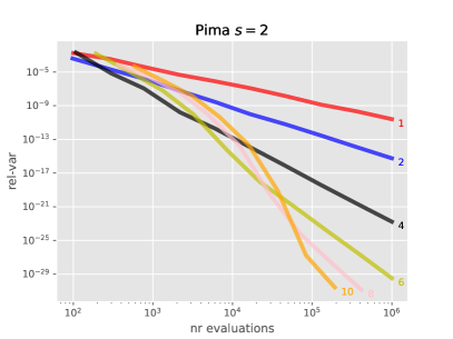
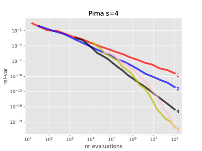
Figure 5: Relative variance of the non-vanishing estimator versus number of evaluations for Pima example when $s=2$ (left) and $s=4$ (right).

When a function $f$ is vanishing, one may use either a vanishing estimator $\widehat{\mathcal{I}}^{0}_{r,k}(f)$ or a non-vanishing estimator $\widehat{\mathcal{I}}_{r,k}(f)$ to compute its integral. One may wonder which type of estimators may lead to better performance. Figure 5 showcases the performance of the non-vanishing estimator when applied to the functions of the previous example for $s=2$ and $s=4$, and should be compared to the top panels of Figure 4.

One sees that, in this particular case, we do obtain better performance with the non-vanishing estimator for $s=2$. (The picture is less clear for $s=4$.) On the other hand, note that the non-vanishing estimator is less convenient to use. As we explained in the previous example and in Section 4.2, one can compute simultaneously the vanishing estimators at orders 1 to some $r_{\max}$. It is then possible to select the order that leads to best performance (using the variance estimator described in Section 4.1). On the other hand, the left panel of Figure 5 shows clearly that one does not know in advance which value of $r$ may lead to best performance when using the non-vanishing estimator.

Appendix C Proofs

C.1 Proof of Lemma 2

We consider first the univariate case: $s=1$, $g\in\mathcal{C}^{r}([0,1])$. Let

$$\mathfrak{C}_{k}^{(1)}:=\left\{\frac{2j+1}{2k}\text{ s.t. }\,j\in\{0,\dots,k-1\}\right\}$$

which is $\mathfrak{C}_{k}$ when $s=1$, and let $l\geq 2$ be an integer, $k\geq l$,

$$S_{l}:=\left\{\kappa\in\{-l+1,\dots,l-1\}^{l}:\,\kappa_{i}\neq\kappa_{j},\,\,\forall i\neq j\right\}$$

and $V_{l}:=\left\{A^{-1}_{\kappa}e^{(a)}:\,\ \kappa\in S_{l},\,a\in\{1,\dots,l-1\}\right\}$ with $A_{\kappa}$ and $e^{(a)}$ as defined in Lemma 1 (with $r=l$).

Let

$$\tilde{C}_{l}=\max_{\{w_{j}\}_{j=1}^{l}\in V_{l},\,\{\kappa_{j}\}_{j=1}^{k}\in S_{l}}\sum_{j=1}^{l}|w_{j}\kappa_{j}^{l}|.$$

Then, by Lemma 1, for all $c^{\prime}\in\mathfrak{C}_{k}^{(1)}$, all $\kappa\in S_{l}$ such that $c^{\prime}+\kappa_{j}/k\in[0,1]$ for all $j\in\{1,\dots,l\}$, and all $a\in\{1,\dots,l-1\}$, there exists a set $\{w^{(a,c^{\prime})}_{j}\}_{j=1}^{l}\in V_{l}$ such that

$$\left|g^{(a)}(c^{\prime})-\frac{\sum_{j=1}^{l}w^{(a,c^{\prime})}_{j}g(c^{\prime}+\kappa_{j}/k)}{k^{-a}}\right|\leq k^{-(l-a)}\|g\|_{l}\tilde{C}_{l}.$$ (22)

We let $\mathcal{W}_{r}=\cup_{j=2}^{r}V_{j}$. We now consider the multivariate case, $s\geq 2$, and prove the lemma by induction on $|\alpha|_{0}$.

To this aim, let $\alpha$ be such that $|\alpha|_{0}=1$, $c=(c_{1},\dots,c_{s})\in\mathfrak{C}_{k}$, $p\in\{1,\dots,s\}$ such that $\alpha_{p}=1$ and $g_{c}\in\mathcal{C}^{r}([0,1])$ defined as (with obvious convention when $p\in\{1,s\}$)

$$g_{c}(c^{\prime}):=f\left(c_{1},\dots,c_{p-1},c^{\prime},c_{p+1},\dots,c_{s}\right),\quad\forall c^{\prime}\in[0,1].$$

Next, let $\{c^{\prime}_{j}\}_{j=1}^{r}$ be $r$ distinct elements of $\mathfrak{C}_{k}^{(1)}$ such that $|c_{p}-c^{\prime}_{j}|\leq(r-1)/k$ for all $j\in\{1,\dots,r\}$, and let $\kappa^{\alpha}_{j}=k(c_{j}-c_{p})$ for all $j$. Note that the resulting vector $\kappa^{\alpha}$ is such that $\kappa^{\alpha}\in S_{r}$. Then, applying (22) with $l=r$, $a=|\alpha|$, $c^{\prime}=c_{p}$, $\kappa=\kappa^{\alpha}$ and $g=g_{c}$, it follows that there exists a set $\{w^{\alpha}_{j}\}_{j=1}^{r}\in V_{r}$ such that

$$\left|D^{\alpha}f(c)-\frac{\sum_{j=1}^{r}w^{\alpha}_{j}g_{c}(c^{\prime}_{j})}{k^{-|\alpha|}}\right| =\left|g_{c}^{(|\alpha|)}(c_{p})-\frac{\sum_{j=1}^{r}w^{\alpha}_{j}g_{c}(c_{j_{\alpha}}+\kappa_{j}/k)}{k^{-a}}\right|$$

$$\leq k^{-(r-|\alpha|)}\|g_{c}\|_{r}\tilde{C}_{r}$$

$$\leq k^{-(r-|\alpha|)}\|f\|_{r}\tilde{C}_{r}.$$ (23)

Then, since $c^{\prime}_{j}\in\mathfrak{C}_{k}^{(1)}$ for all $j\in\{1,\dots,r\}$ if follows that there exist a set $\{c^{(j)}\}_{j=1}^{r}\in\mathfrak{C}_{k}$ such that $g_{c}(c^{\prime}_{j})=f(c^{(j)})$ for all $j\in\{1,\dots,r\}$. Noting that $r=\prod_{i=1}^{|\alpha|_{0}}(r-i+1)$ if $|\alpha|_{0}=1$, the conclusion of the lemma holds with $C_{|\alpha|,s}=\tilde{C}_{r}$ for an $\alpha$ such that $|\alpha|_{0}=1$.

We now let $\alpha$ be such that $|\alpha|_{0}\geq 2$ and $\alpha^{\prime}\in\mathbb{N}_{0}^{s}$ be such that $|\alpha^{\prime}|_{0}=|\alpha|_{0}-1$ and such that there exists a unique $p\in\{1,\dots,s\}$ for which $\alpha^{\prime}_{j}=\alpha_{j}$ for all $j\neq p$. Let $c=(c_{1},\dots,c_{s})\in\mathfrak{C}_{k}$ and $g_{c}\in\mathcal{C}^{r-|\alpha|^{\prime}}([0,1])$ be defined by (with obvious convention when $p\in\{1,s\}$)

$$g_{c}(c^{\prime})=D^{\alpha^{\prime}}f\left(c_{1},\dots,c_{p-1},c^{\prime},c_{p+1},\dots,c_{s}\right),\quad c^{\prime}\in[0,1].$$

Note that $|\alpha|=|\alpha^{\prime}|+\alpha_{p}$, and thus $D^{\alpha}f(c)=g^{(\alpha_{p})}(c_{p})$.

We now let $\{c^{\prime}_{j}\}_{j=1}^{r-|\alpha^{\prime}|}$ be $r-|\alpha^{\prime}|$ distinct elements of the set $\mathfrak{C}_{k}^{(1)}$ such that $|c_{p}-c^{\prime}_{j}|\leq(r-|\alpha^{\prime}|-1)/k$ for all $j\in\{1,\dots,r-|\alpha^{\prime}|\}$, and $\kappa^{\alpha}_{j}=k(c_{j}-c_{p})$ for all $j$. Note that the resulting vector $\kappa^{\alpha}$ is such that $\kappa^{\alpha}\in S_{r-|\alpha^{\prime}|}$ and let $\{c^{(j)}\}_{j=1}^{r-|\alpha^{\prime}|}\subset\mathfrak{C}_{k}$ be such that (with obvious convention when $p\in\{1,s\}$)

$$c^{(j)}=(c_{1},\dots,c_{p-1},c^{\prime}_{j},c_{p+1},\dots,c_{s}),\quad\forall j\in\{1,\dots,r-|\alpha^{\prime}|\}.$$

Then, applying (22) with $l=r-|\alpha^{\prime}|$, $a=\alpha_{p}$, $c^{\prime}=c_{p}$, $\kappa=\kappa^{(\alpha)}$ and $g=g_{c}$, it follows that there exists a set $\{w^{(p)}_{j}\}_{j=1}^{r-|\alpha^{\prime}|}\in V_{r-|\alpha^{\prime}|}$ such that

$$\begin{split}\left|D^{\alpha}f(c)-\frac{\sum_{j=1}^{r-|\alpha^{\prime}|}w^{(p)}_{j}D^{\alpha^{\prime}}f(c^{(j)})}{k^{-\alpha_{p}}}\right|&=\left|D^{\alpha}f(c)-\frac{\sum_{j=1}^{r-|\alpha^{\prime}|}w^{(p)}_{j}g_{c}(c^{\prime}_{j})}{k^{-\alpha_{p}}}\right|\\ &\leq k^{-(r-|\alpha^{\prime}|-\alpha_{p})}\|g_{c}\|_{r-|\alpha^{\prime}|}\tilde{C}_{r-|\alpha^{\prime}|}\\ &\leq k^{-(r-|\alpha^{\prime}|-\alpha_{p})}\|f\|_{r}\tilde{C}_{r-|\alpha^{\prime}|}\\ &=k^{-(r-|\alpha|)}\|f\|_{r}\tilde{C}_{r-|\alpha^{\prime}|}.\end{split}$$ (24)

To proceed further for $j\in\{1,\dots,r-|\alpha^{\prime}|\}$ let

$$\widehat{D}^{\alpha^{\prime}}f(c^{(j)})=k^{|\alpha^{\prime}|}\sum_{q=1}^{l_{r,\alpha^{\prime}}}w^{(j)}_{q}f(c^{(j,q)})$$

where $\{w^{(j)}_{q}\}_{q=1}^{l_{r,\alpha^{\prime}}}$ and $\{c^{(j,q)}\}_{q=1}^{l_{r,\alpha^{\prime}}}$ verify the conditions of the lemma for $c=c^{(j)}$ and are such that

$$\left|\widehat{D}^{\alpha^{\prime}}f(c^{(j)})-D^{\alpha^{\prime}}f(c^{(j)})\right|\leq k^{-(r-|\alpha^{\prime}|)}\|f\|_{r}C_{|\alpha^{\prime}|,s}$$ (25)

for some constant $C_{|\alpha^{\prime}|,s}<\infty$. By the induction hypothesis, there exist sets $\{w^{(j)}_{q}\}_{q=1}^{l_{r,\alpha^{\prime}}}$ and $\{c^{(j,q)}\}_{q=1}^{l_{r,\alpha^{\prime}}}$ that verify these conditions.

We now let

$$\widehat{D}^{\alpha}_{f}(c)=k^{\alpha_{p}}\sum_{j=1}^{r-|\alpha^{\prime}|}w_{j}^{(p)}\widehat{D}^{(\alpha^{\prime})}_{f}(c^{(j)})$$

and remark that

$$\widehat{D}^{\alpha}_{f}(c) =k^{\alpha_{p}+|\alpha^{\prime}|}\sum_{j=1}^{r-|\alpha^{\prime}|}w_{j}^{(p)}\sum_{q=1}^{l_{r,\alpha^{\prime}}}w^{(j)}_{q}f(c^{(j,q)})$$

$$=k^{|\alpha|}\sum_{j=1}^{(r-|\alpha^{\prime}|)l_{r,\alpha^{\prime}}}\tilde{w}_{j}f(\tilde{c}_{j})=k^{|\alpha|}\sum_{j=1}^{l_{r,\alpha}}\tilde{w}_{j}f(\tilde{c}_{j})$$

where the last equality uses the fact that

$$(r-|\alpha^{\prime}|)l_{r,\alpha^{\prime}}=(r-|\alpha^{\prime}|)\prod_{i=1}^{|\alpha^{\prime}|_{0}}(r-i+1)=\prod_{i=1}^{|\alpha|_{0}}(r-i+1)$$

while the penultimate equality holds for a suitable definition of $\{\tilde{w}_{j}\}_{j=1}^{l_{r,\alpha}}$ and of $\{\tilde{c}_{j}\}_{j=1}^{l_{r,\alpha}}$.

Under the induction hypothesis, each $w^{(j)}_{q}$ is the product of $|\alpha^{\prime}|_{0}$ elements of $\mathcal{W}_{r}$, and since each $w_{j}^{p}$ belongs to this set it follows that each $\tilde{w}_{j}$ is the product of $|\alpha^{\prime}|_{0}+1=|\alpha|_{0}$ elements of $\mathcal{K}_{r}$, as required. It is also clear that, under the induction hypothesis and the conditions on $\{c_{j}\}_{j=1}^{r-|\alpha^{\prime}|}$ imposed above, the set $\{\tilde{c}_{j}\}_{j=1}^{l_{r,\alpha}}$ verifies the assumption of the lemma.

Finally, using (24) and (25), we have

$$\left|D^{\alpha}f(c)-\frac{\sum_{j=1}^{r-|\alpha^{\prime}|}w_{j}^{p}\widehat{D}^{(\alpha^{\prime})}_{f(c_{j})}}{k^{-\alpha_{p}}}\right|\leq \left|D^{\alpha}f(c)-\frac{\sum_{j=1}^{r-|\alpha^{\prime}|}w^{(p)}_{j}D^{\alpha^{\prime}}f(c^{(j)})}{k^{-\alpha_{p}}}\right|$$

$$+\sum_{j=1}^{r-|\alpha^{\prime}|}\frac{w^{p}_{j}}{k^{-\alpha_{p}}}\left|\widehat{D}^{(\alpha^{\prime})}_{f(c_{j})}-D^{\alpha^{\prime}}(c_{j})\right|$$

$$\leq k^{-(r-|\alpha|)}\|f\|_{r}\tilde{C}_{r-|\alpha^{\prime}|}$$

$$+k^{\alpha_{p}}\left(\sum_{j=1}^{r-|\alpha^{\prime}|}|w^{p}_{j}|\right)k^{-(r-|\alpha^{\prime}|)}\|f\|_{r}C_{|\alpha^{\prime}|,s}$$

$$\leq k^{-(r-|\alpha|)}\,\|f\|_{r}\left(\tilde{C}_{r-|\alpha^{\prime}|}+\tilde{C}_{r-|\alpha^{\prime}|}C_{|\alpha^{\prime}|,s}\right)$$

$$\leq k^{-(r-|\alpha|)}\,\|f\|_{r}C_{|\alpha|,s}$$

with $C_{|\alpha|,s}=\tilde{C}_{r-|\alpha^{\prime}|}(1+C_{|\alpha^{\prime}|,s})$. The proof is complete.

C.2 Proof of Lemma 3

Below we only prove the lemma for $\widetilde{\mathcal{I}}_{r,k}(f)$, the proof for $\widehat{\mathcal{I}}_{r,k}(f)$ being identical.

Let $k\geq r$, $c\in\mathfrak{C}_{k}$, and $h_{k,c}:[-1/2k,1/2k]^{s}\rightarrow\mathbb{R}$ be defined as $h_{k,c}(u):=\bar{h}_{k,c}(u)-\mathbb{E}[\bar{h}_{k,c}(U_{c})]$ where

$$\bar{h}_{k,c}(u):=f(c+u)-\sum_{l=1}^{r-1}\sum_{|\alpha|=l}\frac{\widehat{D}^{\alpha}_{k}f(c)}{\alpha!}\left(u^{\alpha}-\prod_{j=1}^{s}d_{k}(\alpha_{j})\right).$$

Then, $\widetilde{\mathcal{I}}_{r,k}(f)=k^{-s}\sum_{c\in\mathfrak{C}_{k}}\bar{h}_{k,c}(U_{c})$ and, since $\mathbb{E}[\widetilde{\mathcal{I}}_{r,k}(f)]=\mathcal{I}(f)$, we have

$$\widetilde{\mathcal{I}}_{r,k}(f)-\mathcal{I}(f)=\frac{1}{k^{s}}\sum_{c\in\mathfrak{C}_{k}}h_{k,c}(U_{c}).$$

To prove the second part of the lemma let $k\geq r$, $c\in\mathfrak{C}_{k}$ and $u\in(-1/2k,1/2k)^{s}$. Then, using (2) and with $R_{f,r}$ as in (3),

$$f(c+u) =f(c)+\sum_{l=1}^{r-1}\sum_{|\alpha|=l}\frac{D^{\alpha}f(c)}{\alpha!}u^{\alpha}+R_{f,r}(c,u)$$

so that

$$\begin{split}h_{k,c}(u)&=\sum_{l=1}^{r-1}\sum_{|\alpha|=l}\frac{D^{\alpha}f(c)-\widehat{D}^{\alpha}_{k}f(c)}{\alpha!}\left(U^{\alpha}_{c}-\prod_{j=1}^{s}d_{k}(\alpha_{j})\right)\\ &+R_{f,r}(c,u)-\mathbb{E}[R_{f,r}(c,U_{c})].\end{split}$$ (26)

To proceed further, remark that for all $\alpha$ we have

$$u^{\alpha}\leq(2k)^{-|\alpha|}$$ (27)

and thus

$$|R_{f,r}(c,u)|\leq k^{-r}2^{-r}\|f\|_{r}\sum_{\alpha:|\alpha|=r}\frac{1}{\alpha!}.$$ (28)

In addition, using (27) and noting that $d_{k}(j)\leq k^{-j}$ for all $j\in\mathbb{N}$, we have

$$\left|u^{\alpha}-\prod_{j=1}^{s}d_{k}(\alpha_{j})\right|\leq(2k)^{-|\alpha|}+k^{-|\alpha|}=k^{-|\alpha|}(2^{-|\alpha|}+1)$$ (29)

while, letting $\bar{C}_{r,s}=\max_{j\in\{1,\dots,r-1\}}C_{j,s}$ with $\{C_{j,s}\}_{j=1}^{r-1}$ as in Lemma 2,

$$|D^{\alpha}f(c)-\widehat{D}^{\alpha}_{k}f(c)|\leq C_{r,s}\|f\|_{r}k^{-(r-|\alpha|)}.$$ (30)

Therefore, using (26) and (28)-(30), it follows that

$$|h_{k,c}(u)|\leq\widehat{C}_{s,r}\|f\|_{r}k^{-r},\quad\forall c\in\mathfrak{C}_{k},\quad\forall u\in(-1/2k,1/2k)^{s}$$ (31)

where

$$\widehat{C}_{s,r}=2C_{r,s}\sum_{l=1}^{r-1}\sum_{|\alpha|=l}\frac{1}{\alpha!}+2^{-r+1}\sum_{\alpha:|\alpha|=r}\frac{1}{\alpha!}.$$

The proof is complete.

C.3 Proof of Lemma 5

We prove the result for the estimator $\widehat{\mathcal{I}}_{r,k}(f)$, the proof for $\widetilde{\mathcal{I}}_{r,k}(f)$ being identical.

Recall that, for $[a,b]\subset[0,1]^{s}$ and $f:[0,1]^{s}\rightarrow\mathbb{R}$, function $f_{[a,b]}:[0,1]^{s}\rightarrow\mathbb{R}$ is defined as

$$f_{[a,b]}(u):=f(a+u(b-a)),\quad u\in[0,1]^{s}$$

where the product $u(b-a)$ must be understood as being component-wise.

We assume without loss of generality that the elements of the set $\{\tilde{B}_{q}\}_{q=1}^{p_{r,k}}$ are labelled so that $\int_{\tilde{B}_{q}\cap\tilde{B}_{q^{\prime}}}\mathrm{d}u=0$ whenever $q,q^{\prime}\leq\lfloor k/r\rfloor^{s}$. (Recall that the number of $\tilde{B}_{q}$ is $p_{r,k}=\lceil k/r\rceil^{s}>\lfloor k/r\rfloor^{s}$ when $k/r\notin\mathbb{N}$.)

Then letting

$$E_{r,k}=[0,1]^{s}\setminus\cup_{q=1}^{\lfloor k/r\rfloor^{s}}\tilde{B}_{q},$$

it follows that

$$\widehat{\mathcal{I}}_{r,k}(f)\stackrel{{\scriptstyle\mathclap{\mbox{\tiny{dist}}}}}{{=}}\frac{r^{s}}{k^{s}}\sum_{q=1}^{\lfloor k/r\rfloor^{s}}\widehat{\mathcal{I}}_{r,r}(f_{\tilde{B}_{q}})+\widehat{\mathcal{I}}_{r,k}(f\mathds{1}_{E_{r,k}}).$$

Since these $\lfloor k/r\rfloor^{s}+1$ terms are independent, we have

$$\begin{split}\mathrm{Var}(\widehat{\mathcal{I}}_{r,k}(f))&=\frac{r^{2s}}{k^{2s}}\sum_{q=1}^{\lfloor k/r\rfloor^{s}}\mathrm{Var}\left(\widehat{\mathcal{I}}_{r,r}(f_{\tilde{B}_{q}})\right)+\mathrm{Var}\left(\widehat{\mathcal{I}}_{r,k}(f\mathds{1}_{E_{r,k}})\right).\end{split}$$ (32)

We now let $q\in\{1,\dots,\lfloor k/r\rfloor^{s}\}$ and follow the same lines as in (haber1969stochastic_bis, Theorem 2) in order to compute $\lim_{p\rightarrow\infty}\mathrm{Var}\left(\widehat{\mathcal{I}}_{r,r}(f_{\tilde{B}_{q}})\right)$.

To this aim let $\tilde{c}_{q}$ denote the centre of $\tilde{B}_{q}$ so that, using Taylor’s theorem, (2), we have for all $u\in[0,1]^{s}$

$$f(u)=\sum_{l=0}^{r}\sum_{\alpha:|\alpha|=l}\frac{D^{\alpha}f(\tilde{c}_{q})}{\alpha!}(u-\tilde{c}_{q})^{\alpha}+R_{f,r}(\tilde{c}_{q},u)$$ (33)

where the function $R_{f,r}$ is such that (Amann et al.,, 2008, Theorem 5.11, p. 187)

$$\lim_{\delta\searrow 0}\,\delta^{-r}\sup_{u,v\in[0,1]^{s}\,:\|u-v\|\leq\delta}|R_{f,r}(u,v-u)|=0.$$ (34)

Next, let $g:[0,1]^{s}\rightarrow\mathbb{R}$ be defined by

$$g(u):=\sum_{\alpha:|\alpha|=r}\frac{D^{\alpha}f(\tilde{c}_{q})}{\alpha!}(u-\tilde{c}_{q})^{\alpha}+R_{f,r}\left(\tilde{c}_{q},u\right),\quad u\in[0,1]^{s}$$

and $h:=f-g$. By Theorem 1, $\widehat{\mathcal{I}}_{r,r}(h_{\tilde{B}_{q}})=v_{q}$ a.s. with $v_{q}:=\int h_{\tilde{B}_{q}}(u)\mathrm{d}u$ since $h$ is a polynomial of degree at most $r-1$. Hence, using (33), we have

$$\widehat{\mathcal{I}}_{r,r}(f_{\tilde{B}_{q}})-v_{q} =\widehat{\mathcal{I}}_{r,r}(g_{\tilde{B}_{q}})$$

$$=\sum_{\alpha:|\alpha|=r}\frac{D^{\alpha}f(\tilde{c}_{q})}{\alpha!}\,\widehat{\mathcal{I}}_{r,r}\left(\{(\cdot-\tilde{c}_{q})^{\alpha}\}_{\tilde{B}_{q}}\right)+\widehat{\mathcal{I}}_{r,r}\left(R_{f,r}(\tilde{c}_{q},\cdot)|_{\tilde{B}_{q}}\right)$$

$$=\frac{r^{r}}{k^{r}}\sum_{\alpha:|\alpha|=r}\frac{D^{\alpha}f(\tilde{c}_{q})}{\alpha!}\widehat{\mathcal{I}}_{r,r}\left((\cdot-1/2)^{\alpha}\right)+\widehat{\mathcal{I}}_{r,r}\left(r_{k,q}\right)$$

where the function $r_{k,q}$ is defined as $r_{k,q}(u):=R_{f,r}(\tilde{c}_{q},\tilde{c}_{q}-r/(2k)+ur/k)$ for $u\in[0,1]^{s}$.

This implies that

$$\mathbb{E}\big{[}\widehat{\mathcal{I}}_{r,r}(g_{\tilde{B}_{q}})\big{]} =\frac{r^{r}}{k^{r}}\sum_{\alpha:|\alpha|=r}\frac{D^{\alpha}f(\tilde{c}_{q})}{\alpha!}\int_{[0,1]^{s}}(u-1/2)^{\alpha}\mathrm{d}u+\int_{[0,1]^{s}}r_{k,q}(u)\mathrm{d}u$$

and letting

$$M_{\alpha} :=\widehat{\mathcal{I}}_{r,r}\left((\cdot-1/2)^{\alpha}\right)-\int_{[0,1]^{s}}(u-1/2)^{\alpha}\mathrm{d}u$$

$$R_{k,q} :=\widehat{\mathcal{I}}_{r,r}(r_{k,q})-\int_{[0,1]^{s}}r_{k,q}(u)du$$

for all $\alpha$ such that $|\alpha|=r$, we have

$$\mathrm{Var}\left(\widehat{\mathcal{I}}_{r,r}(f_{\tilde{B}_{q}})\right)= \mathbb{E}\left[\left\{\frac{r^{r}}{k^{r}}\sum_{\alpha:|\alpha|=r}\frac{D^{\alpha}f(c)}{\alpha!}M_{\alpha}+R_{k,q}]\right\}^{2}\right]$$

$$= \frac{r^{2r}}{k^{2r}}\sum_{\alpha,\,\alpha^{\prime}:|\alpha|=|\alpha^{\prime}|=r}\frac{D^{\alpha}f(c)}{\alpha!}\frac{D^{\alpha}f(c)}{\alpha^{\prime}!}\mathbb{E}[M_{\alpha}M_{\alpha^{\prime}}]+\mathrm{Var}(R_{k,q})$$

$$+\frac{2r^{r}}{k^{r}}\sum_{\alpha:|\alpha|=r}\frac{D^{\alpha}f(c)}{\alpha!}\,\mathbb{E}\left[M_{\alpha}R_{k,q}\right].$$

The above computations show that

$$\begin{split}k^{s+2r}\,&\left(\frac{r^{2s}}{k^{2s}}\sum_{q=1}^{\lfloor k/r\rfloor^{s}}\mathrm{Var}\left(\widehat{\mathcal{I}}_{r,r}(f_{\tilde{B}_{q}})\right)\right)\\ =&r^{2r+s}\sum_{\alpha,\,\alpha^{\prime}:|\alpha|=|\alpha^{\prime}|=r}\mathbb{E}[M_{\alpha}M_{\alpha^{\prime}}]\left(\frac{r^{s}}{k^{s}}\sum_{q=1}^{\lfloor k/r\rfloor^{s}}\frac{D^{\alpha}f(\tilde{c}_{q})}{\alpha!}\frac{D^{\alpha}f(\tilde{c}_{q})}{\alpha^{\prime}!}\right)\\ &+r^{2s}k^{2r-s}\sum_{q=1}^{\lfloor k/r\rfloor^{s}}\mathrm{Var}(R_{k,q})\\ &+2r^{r+2s}k^{r-s}\sum_{q=1}^{\lfloor k/r\rfloor^{s}}\sum_{\alpha:|\alpha|=r}\frac{D^{\alpha}f(c)}{\alpha!}\,\mathbb{E}\left[M_{\alpha}R_{k,q}\right]\end{split}$$ (35)

and we now study in turn each of these three terms.

To study the first term recall that $B_{k}(c)$ denotes the hypercube of volume $k^{-s}$ and centre $c\in\mathfrak{C}_{k}$, and let $\{c_{j}\}_{j=1}^{k^{s}-\lfloor k/r\rfloor^{s}r^{s}}$ be the $k^{s}-\lfloor k/r\rfloor^{s}r^{s}$ elements of $\mathfrak{C}_{k}$ such that

$$\int_{B_{k}(c_{j})\cap\tilde{B}_{q}}\mathrm{d}u=0,\quad\forall j\in\{1,\dots,k^{s}-\lfloor k/r\rfloor^{s}r^{s}\},\quad\forall q\in\{1,\dots,\lfloor k/r\rfloor^{s}\}$$

and such that

$$\left(\bigcup_{j=1}^{k^{s}-\lfloor k/r\rfloor^{s}r^{s}}B_{k}(c_{j})\right)\bigcup\left(\bigcup_{q=1}^{\lfloor k/r\rfloor^{s}}\tilde{B}_{q}\right)=[0,1]^{s},$$

and let $\alpha$ and $\alpha^{\prime}$ be such that $|\alpha|=|\alpha^{\prime}|=r$. Then, since

$$\limsup_{k\rightarrow\infty}\left|\frac{1}{k^{s}}\sum_{j=1}^{k^{s}-\lfloor k/r\rfloor^{s}r^{s}}D^{\alpha}f(c_{j})\,D^{\alpha^{\prime}}f(c_{j})\right| \leq\limsup_{k\rightarrow\infty}\frac{k^{s}-\lfloor k/r\rfloor^{s}r^{s}}{k^{s}}\|f\|_{r}$$

$$\leq\|f\|_{r}\limsup_{k\rightarrow\infty}\left(1-(1-r/k)^{s}\right)=0$$

and because the Riemann sum

$$\frac{r^{s}}{k^{s}}\sum_{q=1}^{\lfloor k/r\rfloor^{s}}D^{\alpha}f(\tilde{c}_{q})\,D^{\alpha^{\prime}}f(\tilde{c}_{q})+\frac{1}{k^{s}}\sum_{j=1}^{k^{s}-\lfloor k/r\rfloor^{s}r^{s}}D^{\alpha}f(c_{j})\,D^{\alpha^{\prime}}f(c_{j})$$

converges to $\int_{[0,1]^{s}}D^{\alpha}f(u)\,D^{\alpha^{\prime}}f(u)\mathrm{d}u$ as $k\rightarrow\infty$, it follows that

$$\lim_{k\rightarrow\infty}\left\{\frac{r^{s}}{k^{s}}\sum_{q=1}^{\lfloor k/r\rfloor^{s}}D^{\alpha}f(\tilde{c}_{q})\,D^{\alpha^{\prime}}f(\tilde{c}_{q})\right\}=\int_{[0,1]^{s}}D^{\alpha}f(u)\,D^{\alpha^{\prime}}f(u)\mathrm{d}u.$$ (36)

Next, using (34) we have

$$\limsup_{k\rightarrow\infty}\left\{k^{2r-s}\sum_{q=1}^{\lfloor k/r\rfloor^{s}}\mathrm{Var}(R_{k,q})\right\} \leq r^{-s}\times\limsup_{k\rightarrow\infty}\left\{k^{2r}\max_{1\leq q\leq\lfloor k/r\rfloor^{s}}\mathbb{E}[R_{k,q}^{2}]\right\}$$

$$=0.$$ (37)

Finally, noting that for some constant $C<\infty$ we have, $\mathbb{P}$-a.s., $|M_{\alpha}|\leq C$ for all $\alpha$ such that $|\alpha|=r$, it follows that

$$\limsup_{k\rightarrow\infty}\left|k^{r-s}\sum_{q=1}^{\lfloor k/r\rfloor^{s}}\sum_{\alpha:|\alpha|=r}\frac{D^{\alpha}f(\tilde{c}_{q})}{\alpha!}\,\mathbb{E}\left[M_{\alpha}R_{k,q}\right]\right|\\ \leq 2Cr^{-s}\|f\|_{r}\left(\sum_{\alpha:|\alpha|=r}\frac{1}{\alpha!}\right)\limsup_{k\rightarrow\infty}\left\{k^{r}\max_{1\leq q\leq\lfloor k/r\rfloor^{s}}\mathbb{E}[|R_{k,q}|]\right\}=0$$ (38)

where the equality holds by (34).

Therefore, combining (35)-(38), we obtain

$$\lim_{k\rightarrow\infty}k^{s+2r}\,\left\{\frac{r^{2s}}{k^{2s}}\sum_{q=1}^{\lfloor k/r\rfloor^{s}}\mathrm{Var}\left(\widehat{\mathcal{I}}_{r,r}(f_{\tilde{B}_{q}})\right)\right\}\\ =r^{2r+s}\sum_{\alpha,\,\alpha^{\prime}:|\alpha|=|\alpha^{\prime}|=r}\frac{\mathbb{E}[M_{\alpha}M_{\alpha^{\prime}}]}{\alpha!\alpha^{\prime}!}\int_{[0,1]^{s}}D^{\alpha}f(u)\,D^{\alpha^{\prime}}f(u)\mathrm{d}u$$ (39)

and thus, by (32), to conclude the proof of the lemma it remains to show that

$$\lim_{k\rightarrow\infty}\left\{k^{s+2r}\mathrm{Var}\left(\widehat{\mathcal{I}}_{r,k}(f\mathds{1}_{E_{r,k}})\right)\right\}=0.$$ (40)

To this aim let $m_{k}:=p_{r,k}-\lfloor k/r\rfloor^{s}$, $\{c_{j}\}_{j=1}^{m_{k}}$ be such that $\cup_{j=1}^{m_{k}}B_{k}(c_{j})=E_{r,k}$ and note that

$$\frac{k^{s}}{m_{k}}\widehat{\mathcal{I}}_{r,k}(f\mathds{1}_{E_{r,k}})= \frac{1}{m_{k}}\sum_{j=1}^{m_{k}}\frac{f(c_{j}+U_{c_{j}})+f(c_{j}-U_{c_{j}})}{2}$$

$$-\frac{1}{m_{k}}\sum_{j=1}^{m_{k}}\sum_{l=1}^{\lfloor(r-1)/2\rfloor}\sum_{\alpha:\,|\alpha|=2l}\frac{\widehat{D}^{\alpha}_{k,f(c_{j})}}{\alpha!}\left(U^{\alpha}_{c_{j}}-\prod_{j=1}^{s}d_{k}(\alpha_{j})\right).$$

Then, using Lemma 3

$$\mathrm{Var}\left((k^{s}/m_{k})\widehat{\mathcal{I}}_{r,k}(f\mathds{1}_{E_{r,k}})\right) \leq\widehat{C}^{2}_{s,r}\|f\|^{2}_{r}m_{k}^{-1}k^{-2r}$$

$$\Leftrightarrow\mathrm{Var}\left(\widehat{\mathcal{I}}_{r,r}(f_{E_{r,k}}\right)\leq m_{k}k^{-2s-2r}\widehat{C}^{2}_{s,r}\|f\|^{2}_{r}$$

where $\widehat{C}_{s,r}<\infty$ is as in Lemma 3.

Therefore, noting that

$$m_{k}=\lceil k/r\rceil^{s}-\lfloor k/r\rfloor^{s}\leq k^{s}\left\{(r^{-1}+k^{-1})^{s}-(r^{-1}-k^{-1})^{s}\right\},$$

we have

$$\limsup_{k\rightarrow\infty}\left\{k^{2r+s}\mathrm{Var}\left(\widehat{\mathcal{I}}_{r,r}(f_{E_{r,k}})\right)\right\}\\ \leq\limsup_{k\rightarrow\infty}\left\{(r^{-1}+k^{-1})^{s}-(r^{-1}-k^{-1})^{s}\right\}\widehat{C}^{2}_{s,r}\|f\|^{2}_{r}=0.$$

This shows (40) and the proof of the lemma is complete.

C.4 Proof of Lemma 6

Recall that $B_{k}(c)$ denotes the hyper-cube $[c-1/2k,c+1/2k]=\prod_{i=1}^{s}[c_{i}-1/2k,c_{i}+1/2k]$, with centre $c$ and volume $k^{-s}$. Treating $k$ as fixed from now on, we define for $j\in\mathbb{N}_{0}$, $\mathcal{B}_{j,1}=\{B_{k}(c)\}_{c\in\mathfrak{C}_{j,k}}$, and, for $l=3,5,\ldots$, we define $\mathcal{B}_{j,l}$ to be the set of hyper-cubes $B_{k/l}(c)$, which are then unions of $l^{s}$ elements in $\mathcal{B}_{j,1}$. We also treat as fixed $\lambda\in\{\pm(2i+1),\,i\in\mathbb{N}_{0}\}$, $p=(|\lambda|-1)$ and $m\geq p/2$.

Consider a given $c\in\mathfrak{C}_{m,k}$. We have $[c-\lambda/2k,c+\lambda/2k]\in\mathcal{B}_{m,|\lambda|}$ and thus there exist distinct hypercubes $\{B_{c,l}\}_{l=1}^{|\lambda|^{s}}$ in $\mathcal{B}_{m,1}$ such that

$$[c-\lambda/2k,c+\lambda/2k]=\bigcup_{l=1}^{|\lambda|^{s}}B_{c,l}.$$

For $U_{c}\sim\mathcal{U}([-1/2k,1/2k]^{s})$, $\bar{g}$ defined as in the statement of the lemma, we have

$$\mathbb{E}[\bar{g}(c+\lambda U_{c})] =k^{s}\int_{[-1/2k,1/2k]^{s}}\bar{g}(c+\lambda u)\mathrm{d}u$$

$$=\frac{k^{s}}{|\lambda|^{s}}\int_{[0,1]^{s}\cap[c-\lambda/2k,c+\lambda/2k]}g(u)\mathrm{d}u$$

$$=\frac{k^{s}}{|\lambda|^{s}}\sum_{l=1}^{|\lambda|^{s}}\int_{[0,1]^{s}\cap B_{c,l}}g(u)\mathrm{d}u.$$ (41)

To proceed further we remark that (again, recall $m\geq p/2$, otherwise this would not be true):

$$\bigcup_{c\in\mathfrak{C}_{m,k}}\left\{[0,1]^{s}\cap\cup_{l=1}^{|\lambda|^{s}}B_{c,l}\right\}=\underbrace{\mathcal{B}_{0,1}\cup\dots\cup\mathcal{B}_{0,1}}_{\text{$|\lambda|^{s}$ times}}$$

which, together with (41), yields

$$\frac{1}{k^{s}}\sum_{c\in\mathfrak{C}_{m,k}}\mathbb{E}[\bar{g}(c+\lambda U_{c})] =\frac{1}{|\lambda|^{s}}\sum_{c\in\mathfrak{C}_{m,k}}\sum_{l=1}^{|\lambda|^{s}}\int_{[0,1]^{s}\cap B_{c,l}}g(u)\mathrm{d}u$$

$$=\sum_{B\in\mathcal{B}_{0,1}}\int_{B}g(u)\mathrm{d}u$$

$$=\int_{[0,1]^{s}}g(u)\mathrm{d}u.$$

The proof is complete.

References

- Amann et al., (2008) Amann, H., Escher, J., and Brookfield, G. (2008). Analysis II. Springer.
- Andrieu and Roberts, (2009) Andrieu, C. and Roberts, G. O. (2009). The pseudo-marginal approach for efficient Monte Carlo computations. Ann. Statist., 37(2):697–725.
- Baer, (2018) Baer, M. (2018). findiff software package. https://github.com/maroba/findiff.
- Bardenet and Hardy, (2020) Bardenet, R. and Hardy, A. (2020). Monte carlo with determinantal point processes. The Annals of Applied Probability, 30(1):368–417.
- Baydin et al., (2017) Baydin, A. l. m. G., Pearlmutter, B. A., Radul, A. A., and Siskind, J. M. (2017). Automatic differentiation in machine learning: a survey. J. Mach. Learn. Res., 18:Paper No. 153, 43.
- Billingsley, (1995) Billingsley, P. (1995). Probability and measure. 3rd ed., Wiley.
- Chopin and Ridgway, (2017) Chopin, N. and Ridgway, J. (2017). Leave Pima Indians alone: binary regression as a benchmark for Bayesian computation. Statist. Sci., 32(1):64–87.
- Constantine and Savits, (1996) Constantine, G. and Savits, T. (1996). A multivariate faa di bruno formula with applications. Transactions of the American Mathematical Society, 348(2):503–520.
- Dick, (2011) Dick, J. (2011). Higher order scrambled digital nets achieve the optimal rate of the root mean square error for smooth integrands. The Annals of Statistics, 39(3):1372–1398.
- Ermakov and Zolotukhin, (1960) Ermakov, S. M. and Zolotukhin, V. (1960). Polynomial approximations and the monte-carlo method. Theory of Probability & Its Applications, 5(4):428–431.
- Haber, (1966) Haber, S. (1966). A modified Monte-Carlo quadrature. Mathematics of Computation, 20(95):361–368.
- Haber, (1967) Haber, S. (1967). A modified Monte-Carlo quadrature. ii. Mathematics of Computation, 21(99):388–397.
- Haber, (1969) Haber, S. (1969). Stochastic quadrature formulas. Mathematics of Computation, 23(108):751–764.
- Krieg and Novak, (2017) Krieg, D. and Novak, E. (2017). A universal algorithm for multivariate integration. Foundations of Computational Mathematics, 17(4):895–916.
- Loomis and Sternberg, (1968) Loomis, L. H. and Sternberg, S. (1968). Advanced calculus. Jones and Bartlett Publishers.
- Novak, (1988) Novak, E. (1988). Deterministic and stochastic error bounds in numerical analysis, volume 1349. Springer.
- Novak, (2016) Novak, E. (2016). Some results on the complexity of numerical integration. Monte Carlo and Quasi-Monte Carlo Methods, pages 161–183.
- Pan and Owen, (2022) Pan, Z. and Owen, A. B. (2022). Super-polynomial accuracy of multidimensional randomized nets using the median-of-means. arXiv 2208.05078.
- Patterson, (1987) Patterson, T. (1987). On the construction of a practical ermakov-zolotukhin multiple integrator. In Numerical Integration, pages 269–290. Springer.
- Robbins and Monro, (1951) Robbins, H. and Monro, S. (1951). A stochastic approximation method. Ann. Math. Statistics, 22:400–407.
- Siegel and O’Brien, (1985) Siegel, A. F. and O’Brien, F. (1985). Unbiased monte carlo integration methods with exactness for low order polynomials. SIAM journal on scientific and statistical computing, 6(1):169–181.
- Sloan and Woźniakowski, (1998) Sloan, I. H. and Woźniakowski, H. (1998). When are quasi-monte carlo algorithms efficient for high dimensional integrals? Journal of Complexity, 14(1):1–33.