Event-Triggered Safe Stabilizing Boundary Control for the Stefan PDE System with Actuator Dynamics

Abstract

This paper proposes an event-triggered boundary control for the safe stabilization of the Stefan PDE system with actuator dynamics. The control law is designed by applying Zero-Order Hold (ZOH) to the continuous-time safe stabilizing controller developed in our previous work. The event-triggering mechanism is then derived so that the imposed safety conditions associated with high order Control Barrier Function (CBF) are maintained and the stability of the closed-loop system is ensured. We prove that under the proposed event-triggering mechanism, the so-called “Zeno” behavior is always avoided, by showing the existence of the minimum dwell-time between two triggering times. The stability of the closed-loop system is proven by employing PDE backstepping method and Lyapunov analysis. The efficacy of the proposed method is demonstrated in numerical simulation.

I Introduction

Safety is an emerging notion in control systems, ensuring required constraints in the state, which is a significant property in numerous industrial applications including autonomous driving and robotics. Classically, such a constrained control design has been treated by model predictive control [1], reference governor [2], reachability analysis [3], etc. Following the pioneering work by Ames, et. al [4], the concept of Control Barrier Function (CBF) and the safe control design by CBF using Quadratic Programming (QP) have been widely spread to the control community, such as robust CBF [5], adaptive CBF [6], fixed-time CBF [7]. The system is said to be safe if the required safe set is forward invariant, guaranteeing the positivity of CBF.

While most of the research in safe/constrained control has focused on the systems described by Ordinary Differential Equations (ODEs), a few recent works have been developing and analyzing the safety or state constraints in the systems described by Partial Differential Equations (PDEs), where the safety in the infinite-dimensional state needs to be satisfied, such as for distributed concentration [8], gas density [9], or the liquid level [10]. Our recent work [11] has incorporated the concept of CBF into the boundary control of a PDE system, the so-called ”Stefan system” [12, 13], which is a representative model for the thermal melting process [14] and biological growth process [15]. We have designed the nonovershooting control [16] to achieve both safety and stabilization of the system around the setpoint, and also developed a CBF-QP safety filter for a given nominal control input. The proposed control law is given in continuous time; however, many practical control systems do not afford sufficiently high frequency in the actuator to justify the continuous-time control input.

Some practical technologies own constraints in sensors and systems with respect to energy, communication, and computation, which require the execution of control tasks when they are necessary [17]. To deal with this problem, the digital control design should be aimed to reduce the number of closing the loop based on the system state, developed as event-triggered control. Pioneering work on event-triggered control is designed for PID controllers in [18]. Following the literature, authors of [19] have demonstrated the advantages of event-driven control over time-driven control for stochastic systems. The authors in [20] proposed event-triggered scheduling to stabilize systems by a feedback mechanism. Subsequent works [21, 22] proposed novel state feedback and output feedback controllers for linear and nonlinear time-invariant systems. Unlike the former literature, [23] and [24] have regarded the closed-loop system under the event-triggered control as a hybrid system and guaranteed asymptotical stability with relaxed conditions for the triggering mechanism. To utilize the effect of this relaxation, dynamic triggering mechanisms are presented in [25].

While all the studies of the event-triggered control mentioned above are for ODE systems, authors of [26] and [27] proposed event-triggered in-domain control for hyperbolic PDE systems, and authors of [28] proposed event-triggered boundary control for hyperbolic PDE systems. Following these studies, [29] developed an event-triggered boundary controller for a reaction-diffusion PDE, and [30] derived an adaptive event-triggered control for a hyperbolic PDE with time-varying moving boundary with bounded velocity. As a state-dependent moving boundary PDE, an event-triggered control has been developed to stabilize the one-phase Stefan PDE in [31]. However, the event-triggering mechanism in [31] owns a limitation that the upper bound of the dwell-time is identical to the sole condition for sampling-time scheduling developed in [32]. Indeed, the condition of the sampling schedule in [32] serves as the necessary condition for ensuring the required constraint in the Stefan system. While, such a necessary condition has not been clarified in the Stefan system with actuator dynamics considered in [11], which requires the methodology from high-relative-degree CBF for satisfying the state constraint.

The event-triggering mechanism has been developed for the purpose of safety with CBF-based methods in [33], which proves the nonexistence of the so-called “Zeno behavior” by showing the existence of a lower bound of the dwell-time. Following this work, [34] achieves safety under the event-triggering mechanism by ensuring the existence of the minimum bounded interevent time using input-to-state safe barrier functions. The recent study in [35] has proposed the safety-critical event-triggered controller design for general nonlinear ODE systems. In addition, the event-triggered control with high-order CBFs under unknown system dynamics has been handled in [36] by adaptive CBF approach and in [37] by Gaussian Process learning approach. Such digital safe control methods have been applied to spacecraft orbit stabilization [38], network systems [39], and so on. However, the safe event-triggered control for PDE systems has not been established yet.

The contributions of the paper include (i) designing the event-triggered mechanism for the Stefan PDE system with actuator dynamics, so that both the safety and stability are maintained, (ii) and proving the nonexistence of Zeno behavior by showing the existence of the minimum dwell-time between two triggering times. Indeed, this paper provides the first study of the event-triggered boundary control for a PDE system to achieve safety and stability. The safety is shown by employing the high order CBF, and the stability is proven by utilizing PDE backstepping method and Lyapunov analysis.

II Stefan Model and Constraints

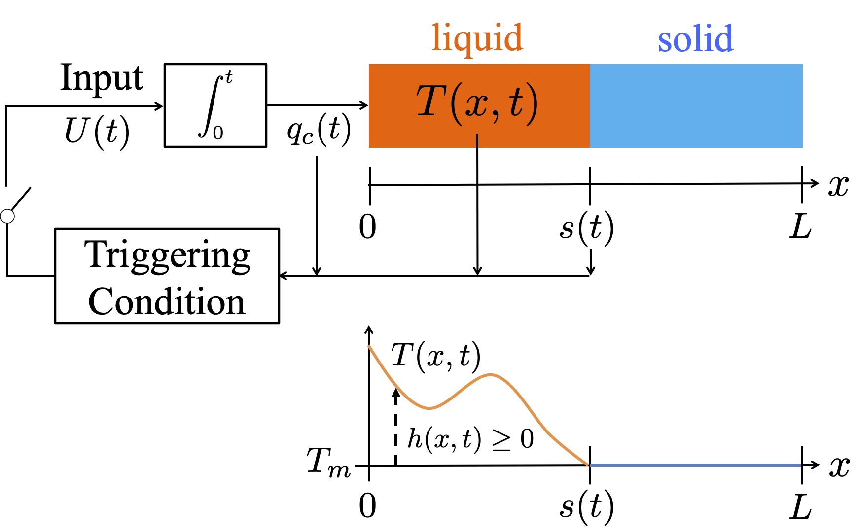
Figure 1: Schematic of the one-phase Stefan problem with actuator dynamics under event-triggered control.

Consider the melting or solidification in a material of length $L$ in one dimension (see Fig. 1). Divide the domain $[0,L]$ into two time-varying sub-intervals: $[0,s(t)]$, which contains the liquid phase, and $[s(t),L]$, that contains the solid phase. Let the heat flux be entering at the boundary of the liquid phase to promote the melting process

The energy conservation and heat conduction laws yield the heat equation of the liquid phase, the boundary conditions, the dynamics of the moving boundary, and the initial values as follows:

$$T_{t}(x,t) =\alpha T_{xx}(x,t),\hskip 5.69054pt\textrm{for}\hskip 5.69054ptt>0,\hskip 5.69054pt0<x<s(t),$$ (1)

$$-kT_{x}(0,t) =q_{\rm c}(t),\hskip 5.69054pt\textrm{for}\hskip 5.69054ptt>0,$$ (2)

$$T(s(t),t) =T_{{\rm m}},\hskip 5.69054pt\textrm{for}\hskip 5.69054ptt>0,$$ (3)

$$\dot{s}(t) =-\beta T_{x}(s(t),t),$$ (4)

$$s(0) =s_{0},\textrm{and }T(x,0)=T_{0}(x),\textrm{for }x\in(0,s_{0}].$$ (5)

The heat flux $q_{\rm c}(t)$ is manipulated by the voltage input $U(t)$ modeled by a first-order actuator dynamics:

$$\dot{q}_{c}(t)=U(t).$$ (6)

There are two requirements for the validity of the model

$$T(x,t)\geq T_{{\rm m}},\quad\forall x\in(0,s(t)),\quad\forall t>0,$$ (7)

$$0<s(t)< L,\quad\forall t>0.$$ (8)

First, the trivial: the liquid phase is not frozen, i.e., the liquid temperature $T(x,t)$ is greater than the melting temperature $T_{\rm m}$. Second, equally trivially, the material is not entirely in one phase, i.e., the interface remains inside the material’s domain. These physical conditions are also required for the existence and uniqueness of solutions [40]. Hence, we assume the following for the initial data.

Assumption 1.

$0<s_{0}<L$, $T_{0}(x)\in C^{1}([0,s_{0}];[T_{\rm m},+\infty))$ with $T_{0}(s_{0})=T_{\rm m}$.

We remark the following lemma.

Lemma 1.

With Assumption 1, if $q_{\rm c}(t)$ is a bounded piecewise continuous non-negative heat function, i.e.,

$$q_{{\rm c}}(t)\geq 0,\quad\forall t\geq 0,$$ (9)

then there exists a unique classical solution for the Stefan problem (1)–(4), which satisfies (7), and

$$\dot{s}(t)\geq 0,\quad\forall t\geq 0.$$ (10)

The definition of the classical solution of the Stefan problem is given in Appendix A of [12]. The proof of Lemma 1 is by maximum principle for parabolic PDEs and Hopf’s lemma, as shown in [40].

Control Barrier Functions (CBFs) are introduced to render the equivalency between the forward invariance of a safe set satisfying the imposed constraints with the positivity of the CBFs. Followng [11], let $h_{1}(t)$, $h_{2}(t)$, $h_{3}(t)$, and $h(x,t)$ be CBFs defined by

$$h_{1}(t): =\sigma(t)$$

$$=-\left(\frac{k}{\alpha}\int_{0}^{s(t)}(T(x,t)-T_{m})dx+\frac{k}{\beta}(s(t)-s_{r})\right),$$ (11)

$$h_{2}(t) =q_{\rm c}(t),$$ (12)

$$h_{3}(t) =-q_{\rm c}(t)+c_{1}\sigma(t),$$ (13)

$$h(x,t) =T(x,t)-T_{\rm m}.$$ (14)

The functions $h_{1}(t)$ and $h_{2}(t)$ defined above can be seen as valid CBFs to satisfy the state constraints in (7) and (8) as shown in the following lemma.

Lemma 2.

With Assumption 1, suppose that the following conditions hold:

$$h_{1}(t)\geq 0,$$ (15)

$$h_{2}(t)\geq 0,$$ (16)

for all $t\geq 0$. Then, it holds that

$$h(x,t)\geq 0,\quad\forall x\in(0,s(t)),\quad\forall t\geq 0,$$ (17)

$$0<s_{0}\leq s(t)\leq s_{r},\quad\forall t\geq 0,$$ (18)

under the classical solution of (1)–(4).

Lemma 2 is proven with Lemma 1. To validate the conditions (15) and (16) for all $t\geq 0$, at least the conditions must hold at $t=0$, which necessitate the following assumptions on the initial condition and the setpoint restriction.

Assumption 2.

$0\leq q_{\rm c}(0)$.

Assumption 3.

The setpoint position $s_{\rm r}$ is chosen to satisfy

$$s_{0}+\frac{\beta}{\alpha}\int_{0}^{s_{0}}(T_{0}(x)-T_{\rm m})dx\leq s_{\rm r}<L.$$ (19)

Note that CBF $h_{3}(t)$ defined in (13) satisfies

$$\dot{h}_{1}(t)=-c_{1}h_{1}(t)+h_{3}(t).$$ (20)

This function is introduced to handle the property that the relative degree of $h_{1}(t)$ is more than 1. We can see it by $\dot{h}_{1}=-q_{\rm c}(t)=-h_{2}(t)$, which is not explicitly dependent on the control input $U(t)$. However, as presented in the next section, the time derivative of $h_{3}(t)$ is explicitly dependent on $U(t)$. Moreover, once the positivity of $h_{3}(t)$ is ensured, then the positivity of $h_{1}(t)$ is also guaranteed owing to (20). Thus, in later sections, for ensuring the safety, we mainly focus on guaranteeing the positivity of $h_{2}(t)$ and $h_{3}(t)$.

III Event-Triggered Control Design

In this section, we propose an event-triggered controller for both safety and stability purposes. [11] develops the nonovershooting control

$$U^{*}(t) =-c_{1}h_{2}(t)+c_{2}h_{3}(t)$$

$$=-(c_{1}+c_{2})q_{\rm c}(t)+c_{1}c_{2}\sigma(t),$$ (21)

under the continuous-time design, where $c_{1}>0$ and $c_{2}>0$ are positive constants satisfying

$$c_{1}\geq\frac{q_{\rm c}(0)}{\sigma(0)}.$$ (22)

The closed-loop system with $U(t)=U^{*}(t)$ is ensured to satisfy the constraints (7) and (8) by showing the positivity of all CBFs, and also shown to be globally exponentially stable.

In this paper, we consider a digital control by applying Zero-Order Hold (ZOH) to the continuous-time control law (III), given as

$$U(t)\equiv U^{*}(t_{j}),\quad\forall t\in[t_{j},t_{j+1}),$$ (23)

and derive a triggering condition for $t_{j}$ to maintain both the safety and stability.

III-A Triggering Condition for Safety

Under (23) with (III), we design the triggering condition so that the following inequalities are satisfied:

$$\dot{h}_{2}(t) \geq-\bar{c}_{1}h_{2}(t),$$ (24)

$$\dot{h}_{3}(t) \geq-\bar{c}_{2}h_{3}(t),$$ (25)

for some positive constants $\bar{c}_{i}>0$. The triggering condition is obtained by using the following procedure.

First, we start with taking time derivative of (11) and (12) and using (6) so, we have

$$\dot{h}_{2}(t) =U(t),$$ (26)

$$\dot{h}_{3}(t) =-U(t)-c_{1}h_{2}(t)$$ (27)

Under the digital control (23), by defining

$$\tilde{U}^{*}(t):=U^{*}(t)-U^{*}(t_{j}),$$ (28)

(26) and (27) yield

$$\dot{h}_{2}(t) =-c_{1}h_{2}(t)+c_{2}h_{3}(t)-\tilde{U}^{*}(t),$$ (29)

$$\dot{h}_{3}(t) =-c_{2}h_{3}(t)+\tilde{U}^{*}(t).$$ (30)

Thus, one can see that to ensure (24) and (25), it must hold

$$(c_{2}-\bar{c}_{2})h_{3}(t)\leq\tilde{U}^{*}(t)\leq(\bar{c}_{1}-c_{1})h_{2}(t)+c_{2}h_{3}(t)$$ (31)

The inequality (31) must be satisfied at least $t=t_{j}$. Noting that $\tilde{U}^{*}(t_{j})=0$ and $h_{2}(t_{j})\geq 0$ and $h_{3}(t_{j})\geq 0$, the parameters $\bar{c}_{1}$ and $\bar{c}_{2}$ introduced in (24) (25) can be set as

$$\bar{c}_{1} =(1+\delta_{1})c_{1}$$ (32)

$$\bar{c}_{2} =(1+\delta_{2})c_{2}$$ (33)

where $\delta_{2}\geq 0$ and $\delta_{1}\geq 0$ are gain parameters. Then, the condition (31) is rewritten as

$$-\delta_{2}c_{2}h_{3}(t)\leq\tilde{U}^{*}(t)\leq\delta_{1}c_{1}h_{2}(t)+c_{2}h_{3}(t)$$ (34)

Then, we can define the set of event times $I={t_{0},t_{1},t_{2},...}$ with $t_{0}=0$ forms an increasing sequence with the following rule by using (34)

$$t_{j+1}=\inf\{\mathcal{S}(t,t_{j})\}$$ (35)

where

$$\mathcal{S}(t,t_{j})=\left\{t\in\mathbb{R}_{+}|\left(t>t_{j}\right)\wedge\left(\left(-\delta_{2}c_{2}h_{3}(t)>\tilde{U}^{*}(t)\right)\right.\right.$$

$$\left.\left.\vee\left(\tilde{U}^{*}(t)>\delta_{1}c_{1}h_{2}(t)+c_{2}h_{3}(t)\right)\right)\right\}.$$ (36)

III-B Triggering Condition for Stability

The event-triggering mechanism for stability can be derived by considering the backstepping approach as follows. Let $X(t)$ be reference error variable defined by $X(t):=s(t)-s_{r}$. Then, the system (1)–(4) is rewritten with respect to $h(x,t)$ defined in (14), $h_{2}(t)$ defined in (12), and $X(t)$ as

$$h_{t}(x,t) =\alpha h_{xx}(x,t),$$ (37)

$$h_{x}(0,t) =-h_{2}(t)/k,$$ (38)

$$\dot{h}_{2}(t) =U(t),$$ (39)

$$h(s(t),t) =0,$$ (40)

$$\dot{X}(t) =-\beta h_{x}(s(t),t).$$ (41)

Following Section 3.3. in [32], we introduce the following forward and inverse transformations:

$$w(x,t) =h(x,t)-\frac{\beta}{\alpha}\int_{x}^{s(t)}\phi(x-y)h(y,t){\rm d}y$$

$$-\phi(x-s(t))X(t),$$ (42)

$$\phi(x) =c_{1}\beta^{-1}x-\varepsilon,$$ (43)

$$h(x,t) =w(x,t)-\frac{\beta}{\alpha}\int_{x}^{s(t)}\psi(x-y)w(y,t){\rm d}y$$

$$-\psi(x-s(t))X(t),$$ (44)

$$\psi(x) =e^{\bar{\lambda}x}\left(p_{1}\sin\left(\omega x\right)+\varepsilon\cos\left(\omega x\right)\right),$$ (45)

where $\bar{\lambda}=\frac{\beta\varepsilon}{2\alpha}$, $\omega=\sqrt{\frac{4\alpha c_{1}-(\varepsilon\beta)^{2}}{4\alpha^{2}}}$, $p_{1}=-\frac{1}{2\alpha\beta\omega}\left(2\alpha c_{1}-(\varepsilon\beta)^{2}\right)$, and $0<\varepsilon<2\frac{\sqrt{\alpha c_{1}}}{\beta}$ is to be chosen later. As derived in Section 3.3. in [32], taking the spatial and time derivatives of (III-B) along the solution of (37)-(41), and noting the CBF $h_{3}(t)$ defined in (13) satisfying (25), one can obtain the following target system:

$$w_{t}(x,t) =\alpha w_{xx}(x,t)+\dot{s}(t)\phi^{\prime}(x-s(t))X(t),$$ (46)

$$w_{x}(0,t) =\frac{h_{3}(t)}{k}-\frac{\beta}{\alpha}\varepsilon\bigg{[}w(0,t)-\frac{\beta}{\alpha}\int_{0}^{s(t)}\psi(-y)w(y,t){\rm d}y$$

$$-\psi(-s(t))X(t)\bigg{]}.$$ (47)

$$\dot{h}_{3}(t) =-c_{2}h_{3}(t)+\tilde{U}^{*}(t),$$ (48)

$$w(s(t),t) =\varepsilon X(t),$$ (49)

$$\dot{X}(t) =-c_{1}X(t)-\beta w_{x}(s(t),t).$$ (50)

Note that (III-B) is derived using $h_{3}(t)=-q_{\rm c}(t)+c_{1}\sigma(t)=-h_{2}(t)-c_{1}\left(\frac{k}{\alpha}\int_{0}^{s(t)}(T(x,t)-T_{\rm m})dx+\frac{k}{\beta}(s(t)-s_{\rm r})\right)\\ =-h_{2}(t)-k\left(\frac{\beta}{\alpha}\int_{0}^{s(t)}\phi^{\prime}(-y)h(y,t)dy+\phi^{\prime}(-s(t))X(t)\right)$, with the helpf of (43). The objective of the transformation (III-B) is to add a stabilizing term $-c_{1}X(t)$ in (50) of the target $(w,X)$-system which is easier to prove the stability than $(u,X)$-system.

We derive the triggering condition to satisfy the following inequality

$$|\tilde{U}^{*}(t)|\leq(1-\delta_{2})c_{2}h_{2}(t)+\delta_{2}c_{2}h_{3}(t),\hskip 8.53581pt\delta_{2}\in(0,1),$$ (51)

which ensures the stability by Lyapunov analysis as shown in the next section. Combining the condition (51) for stability with the condition (34) for safety, the resulting required condition for simultaneous safety and stability is obtained as

$$-\delta_{2}c_{2}h_{3}(t) \leq\tilde{U}^{*}(t)\leq\mu_{1}h_{2}(t)+\delta_{2}c_{2}h_{3}(t),$$ (52)

$$\mu_{1} =\min\{\delta_{1}c_{1},(1-\delta_{2})c_{2}\}$$ (53)

thereby the event-triggering mechanism is described by

$$t_{j+1} =\inf\left\{t\in\mathbb{R}_{+}|\left(t>t_{j}\right)\wedge\left(\left(-\delta_{2}c_{2}h_{3}(t)>\tilde{U}^{*}(t)\right)\right.\right.$$

$$\left.\left.\vee\left(\tilde{U}^{*}(t)>\mu_{1}h_{2}(t)+\delta_{2}c_{2}h_{3}(t)\right)\right)\right\}.$$ (54)

IV Closed-Loop Analysis and Main Results

This section provides the theoretical analysis of the closed-loop system under the proposed event-triggered control law.

IV-A Avoidance of Zeno Behavior

One potential issue of the event-triggered control is the so-called “Zeno” behavior, which causes infinite triggering times within finite time interval. Such behavior essentially does not enable the digital control implementation. The Zeno behavior can be proven not to exist by showing the existence of the minimum dwell-time. We state the following theorem.

Theorem 1.

Let Assumptions 1–3 hold. Consider the closed-loop system consisting of the plant (1)–(6) and the event-triggered boundary control (III) with the gain condition (22) and the triggering mechanism (54). There exists a minimal dwell-time between two triggering times, i.e. there exists a constant $\tau>0$ (independent of the initial condition) such that $t_{j+1}-t_{j}\geq\tau$, for all $j\geq 0$. Moreover, all CBFs defined as (11)–(14) satisfy the constraints $h_{1}(t)\geq 0$, $h_{2}(t)\geq 0$ for all $t\geq 0$, and $h(x,t)\geq 0$ for all $x\in(0,s(t))$ and for all $t\geq 0$.

Proof.

Let $m_{1}(t)$ and $m_{2}(t)$ be defined by

$$m_{1}(t) =\mu_{1}h_{2}(t)+\delta_{2}c_{2}h_{3}(t)-\tilde{U}^{*}(t)$$

$$=(\mu_{1}+c_{1})h_{2}(t)-(1-\delta_{2})c_{2}h_{3}(t)+U^{*}(t_{j}),$$ (55)

$$m_{2}(t) =\tilde{U}^{*}(t)+\delta_{2}c_{2}h_{3}(t)$$

$$=-U^{*}(t_{j})-c_{1}h_{2}(t)+\bar{c}_{2}h_{3}(t).$$ (56)

Since the event-triggering mechanism ensures both $m_{1}(t)>0$ and $m_{2}(t)>0$ for all $t\in[t_{j},t_{j+1})$ and either $m_{1}(t_{j+1})=0$ or $m_{2}(t_{j+1})=0$ holds, we show that there exists a positive constant $\tau>0$ (lower bound of the dwell-time), which is independent on triggered time $t_{j}$, such that both $m_{1}(\bar{t})\geq 0$ and $m_{2}(\bar{t})\geq 0$ hold for some $\bar{t}-t_{j}\geq\tau$. By taking the time derivatives of $m_{1}(t)$ and $m_{2}(t)$, we get

$$\dot{m}_{1}(t) =(\mu_{1}+c_{1}+(1-\delta_{2})c_{2})U^{*}(t_{j})+(1-\delta_{2})c_{1}c_{2}h_{2}(t)$$ (57)

$$\ddot{m}_{1}(t) =(1-\delta_{2})c_{1}c_{2}U^{*}(t_{j})$$ (58)

$$\dot{m}_{2}(t) =-\left(c_{1}+\bar{c}_{2}\right)U^{*}(t_{j})-\bar{c}_{2}c_{1}h_{2}(t),$$ (59)

$$\ddot{m}_{2}(t) =-c_{1}\bar{c}_{2}U^{*}(t_{j}).$$ (60)

Since (58) and (60) are constant in time, explicit solutions for $m_{1}(t)$ and $m_{2}(t)$ with respect to time $t\geq t_{j}$ are obtained as follows.

$$m_{1}(t)= \frac{(1-\delta_{2})c_{1}c_{2}}{2}U^{*}(t_{j})(t-t_{j})^{2}$$

$$+\dot{m}_{1}(t_{j})(t-t_{j})+m_{1}(t_{j})$$

$$= -\frac{(1-\delta_{2})c_{1}c_{2}}{2}(c_{1}h_{2}(t_{j})-c_{2}h_{3}(t_{j}))(t-t_{j})^{2}$$

$$-\left(c_{1}(\mu_{1}+c_{1})h_{2}(t_{j})\right.$$

$$\quad\left.-c_{2}(c_{1}+c_{2}(1-\delta_{2}))h_{3}(t_{j})\right)(t-t_{j})$$

$$+\mu_{1}h_{2}(t_{j})+\delta_{2}c_{2}h_{3}(t_{j})$$ (61)

$$m_{2}(t)= -\frac{c_{1}\bar{c}_{2}U^{*}(t_{j})}{2}(t-t_{j})^{2}+\dot{m}_{2}(t_{j})(t-t_{j})+m_{2}(t_{j})$$

$$= \frac{c_{1}\bar{c}_{2}(c_{1}h_{2}(t_{j})-c_{2}h_{3}(t_{j}))}{2}(t-t_{j})^{2}$$

$$+\left(c_{1}^{2}h_{2}(t_{j})-(c_{1}+\bar{c}_{2})c_{2}h_{3}(t_{j})\right)(t-t_{j})$$

$$+\delta_{2}c_{2}h_{3}(t_{j}).$$ (62)

Owing to the positivity of CBFs $h_{2}(t)$ and $h_{3}(t)$ ensured by (24) and (25) under the event-triggered mechanism (36), the solutions (61) (62) for $t\geq t_{j}$ satisfy the following inequalities:

$$m_{1}(t)\geq h_{2}(t_{j})\left(-\frac{(1-\delta_{2})c_{1}^{2}c_{2}}{2}(t-t_{j})^{2}\right.$$

$$\left.-c_{1}(\mu_{1}+c_{1})(t-t_{j})+\mu_{1}\right),$$ (63)

$$m_{2}(t)\geq c_{2}h_{3}(t_{j})\left(-\frac{c_{1}\bar{c}_{2}}{2}(t-t_{j})^{2}-(c_{1}+\bar{c}_{2})(t-t_{j})+\delta_{2}\right).$$ (64)

One can see that the right hand sides of both (IV-A) and (64) maintain nonnegative for all $t\in[t_{j},t_{j}+\tau)$, where

$$\tau =\min\left\{\tau_{1},\tau_{2}\right\},$$ (65)

$$\tau_{1} =\frac{-c_{1}(\mu_{1}+c_{1})+\sqrt{c_{1}^{2}(\mu_{1}+c_{1})^{2}+2\mu_{1}(1-\delta_{2})c_{1}^{2}c_{2}}}{(1-\delta_{2})c_{1}^{2}c_{2}},$$ (66)

$$\tau_{2} =\frac{-(c_{1}+\bar{c}_{2})+\sqrt{(c_{1}+\bar{c}_{2})^{2}+2\delta_{2}c_{1}\bar{c}_{2}}}{c_{1}\bar{c}_{2}},$$ (67)

which stands as the minimum dwell-time.

∎

IV-B Stability Analysis

We prove the stability of the closed-loop system as presented below.

Theorem 2.

Let Assumptions 1–3 hold. Consider the closed-loop system consisting of the plant (1)–(6) and the event-triggered boundary control (III) with the gain condition (22) and the triggering mechanism (54). The closed-loop system is exponentially stable at the equilibrium $s=s_{\rm r},T(x,\cdot)\equiv T_{\rm m},q_{\rm c}=0$, in the sense of the following norm:

$$\Phi(t):=||T[t]-T_{\rm m}||^{2}+(s(t)-s_{\rm r})^{2}+q_{\rm c}(t)^{2},$$ (68)

for all initial conditions in the safe set, i.e., globally. In other words, there exist positive constants $M>0$ and $b>0$ such that the following norm estimates hold:

$$\Phi(t)\leq M\Phi(0)e^{-bt}.$$ (69)

Proof.

What remains to show is the stability of the system by Lyapunov analysis. Owing to the equivalent stability property through the backstepping transformation, we employ Lyapunov analysis to the target system (46)–(50). Following Lemma 20 in [32], by introducing a Lyapunov function $V(t)$ defined by

$$V(t)=\frac{1}{2\alpha}||w[t]||^{2}+\frac{\varepsilon}{2\beta}X(t)^{2},$$ (70)

one can see that there exists a positive constant $\varepsilon^{*}>0$ such that for all $\varepsilon\in(0,\varepsilon^{*})$ the following inequality holds:

$$\dot{V}(t)\leq -bV(t)+\frac{2s_{\rm r}}{k^{2}}h_{3}(t)^{2}+a\dot{s}(t)V(t),$$ (71)

where $a=\frac{2\beta\varepsilon}{\alpha}\max\left\{1,\frac{\alpha c^{2}s_{{\rm r}}}{2\beta^{3}\varepsilon^{3}}\right\}$, $b=\frac{1}{8}\min\left\{\frac{\alpha}{s_{{\rm r}}^{2}},c\right\}$, and the condition $\dot{s}(t)\geq 0$ ensured in Lemma 1 is applied. We further introduce another Lyapunov function of $h_{3}$, defined by

$$V_{h}(t)=\frac{1}{2}h_{3}(t)^{2}+\frac{q}{2}h_{1}(t)^{2},$$ (72)

with a positive constant $q>0$. Taking the time derivative of (72) and applying (20) and (48) yields

$$\dot{V}_{h}(t)= -c_{2}h_{3}(t)^{2}+h_{3}(t)\tilde{U}^{*}(t)$$

$$+q\left(-c_{1}h_{1}(t)^{2}+h_{1}(t)h_{3}(t)\right).$$ (73)

Under the event-triggered mechanism, the inequality (51) is satisfied, thereby (IV-B) leads to

$$\dot{V}_{h}(t)\leq -c_{2}(1-\delta_{2})h_{3}(t)^{2}+\mu_{1}h_{2}(t)h_{3}(t)$$

$$-qc_{1}h_{1}(t)^{2}+qh_{1}(t)h_{3}(t).$$ (74)

From the definition (13), we have $h_{2}=-h_{3}+c_{1}h_{1}$. Substituting this into (IV-B), applying Young’s inequality to the cross term $h_{1}h_{3}$, one can derive the following inequality:

$$\dot{V}_{h}(t)\leq -\left(c_{2}(1-\delta_{2})+\frac{\mu_{1}}{2}-\frac{q}{2c_{1}}\right)h_{3}(t)^{2}$$

$$-\frac{c_{1}}{2}\left(q-c_{1}\mu_{1}\right)h_{1}(t)^{2}.$$ (75)

Let $\bar{V}$ be the Lyapunov function defined by

$$\bar{V}=V+pV_{h}.$$ (76)

Applying (71) and (IV-B) with setting $q=2c_{1}\mu_{1}$, $p=\frac{8s_{\rm r}}{c_{2}k^{2}(1-\delta_{2})}$, and $\mu_{1}\leq(1-\delta_{2})c_{2}$ by (53), the time derivative of (76) is shown to satisfy

$$\dot{\bar{V}}(t)\leq-\bar{b}\bar{V}(t)+a\dot{s}(t)\bar{V}(t),$$ (77)

where $\bar{b}=\min\{b,2s_{\rm r}/k^{2}\}$. As performed in [32], with the condition $0<s(t)\leq s_{\rm r}$ ensured in Lemma 2, the differential inequality (77) leads to

$$\bar{V}(t)\leq e^{as_{\rm r}}\bar{V}(0)e^{-\bar{b}t},$$ (78)

which ensures the exponential stability of the target system (46)–(50). Due to the invertibility of the transformation (III-B) (III-B), one can show the exponential stability of the closed-loop system, which completes the proof of Theorem 2.

∎

V Simulations

We perform the numerical simulation considering a strip of zinc, the physical parameters of which are given in Table 1 in [12]. The initial interface position is set to $s_{0}=5\ [cm]$, and a linear profile is considered for the initial temperature profile which is $T_{0}(x)=\bar{T}(1-x/s_{0})+T_{\rm m}$ with $\bar{T}=1\ [^{\circ}C]$ and $T_{m}=420\ [^{\circ}C]$. The setpoint position is set as $30\ [cm]$, and control gains are considered as $\delta_{1}=10$, $c_{1}=3.2\times 10^{-3}$ and $c_{2}=0.5\times 10^{-2}$. Fig. 2 depicts the event-based control input under two choices of gain parameters $\delta_{2}=0.3$ and $\delta_{2}=0.7$. The figure illustrates that the input only requires a few number of control updates to ensure stability and safety of the system as opposed to the continuous-time input signal. Fig. 3 demonstrates that the boundary temperature is increased first, then cooled down once the actuator added enough heat and remained positive during this process. In Fig 4, the interface position converges to the setpoint without any overshooting with the proposed control law. Fig. 5, is the imposed CBF for and energy amount, stays positive and satisfies CBF condition. In addition, temperature evolution along the domain is presented in Fig. 6. Starting a linear initial temperature profile, the liquid temperature successfully maintains above the melting temperature with event-triggered control law as the safety of the system. Fig. 7 shows the time-evolution of the control signal with the triggering condition (52). Once the input error $\tilde{U}^{*}(t)$ reaches the lower bound $-\delta_{2}c_{2}h_{3}(t)$ or upper bound $\min(\delta_{1}c_{1},(1-\delta_{2})c_{2})q_{c}(t)+\delta_{2}c_{2}h_{3}(t)$, the triggering event is caused by closing the loop. Then, the input error signal is reset to zero due to the update of the control signal. As a time-evolution, it can be seen that both the lower and upper bounds converge to zero, and the number of events decreases when liquid temperature, $T(x,t)$, converges to the melting temperature, $T_{m}$.

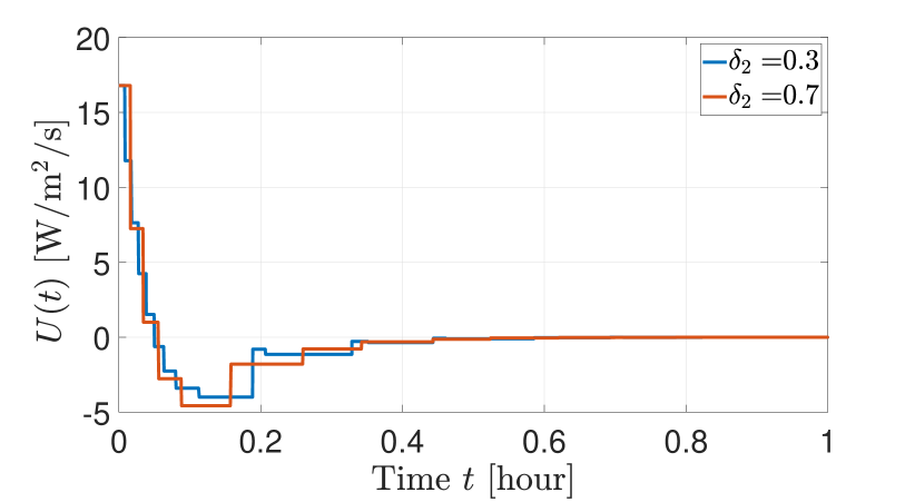
Figure 2: Event-based control input under $\delta_{2}=0.3$ and $\delta_{2}=0.7$.

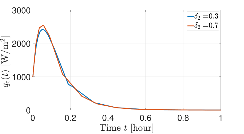
Figure 3: Boundary heat flux remains positive.

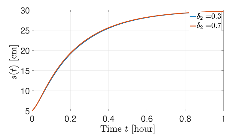
Figure 4: Interface position converges to setpoint without overshooting.

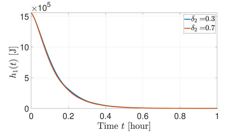
Figure 5: CBF of energy deficit remains positive.

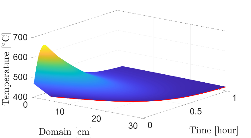
Figure 6: Liquid temperature, $T(x,t)$ remains above the melting temperature and converges to the melting temperature, $T_{m}=420\ [^{\circ}C]$.

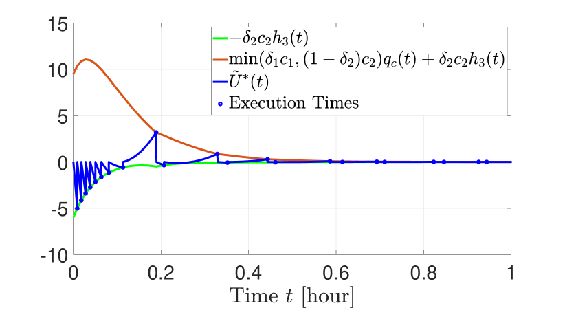
Figure 7: Trajectories involved in the triggering condition (52). Once the trajectory $\tilde{U}^{*}(t)$ reaches the lower bound or upper bounds of (52) an event is generated, the control value is updated and $\tilde{U}^{*}(t)$ is reset to zero.

VI Conclusion

This paper has proposed an event-triggered boundary control for the safety and stability of the Stefan PDE system with actuator dynamics. The control law is designed by applying Zero-Order Hold (ZOH) to the nominal continuous-time feedback control law to satisfy both the safety and stability. The event-triggering mechanism is designed so that the safety and stability are still maintained from the positivity of the imposed CBFs and the stability analysis. Future work includes the development of adaptive event-triggered control to identify unknown parameters [41] and its application to the neuron growth process [15].

References

- [1] L. Hewing, K. P. Wabersich, M. Menner, and M. N. Zeilinger, “Learning-based model predictive control: Toward safe learning in control,” Annual Review of Control, Robotics, and Autonomous Systems, vol. 3, pp. 269–296, 2020.
- [2] E. Gilbert and I. Kolmanovsky, “Nonlinear tracking control in the presence of state and control constraints: a generalized reference governor,” Automatica, vol. 38, no. 12, pp. 2063–2073, 2002.
- [3] S. Bansal, M. Chen, S. Herbert, and C. Tomlin, “Hamilton-jacobi reachability: A brief overview and recent advances,” in 2017 IEEE 56th Annual Conference on Decision and Control (CDC), pp. 2242–2253, IEEE, 2017.
- [4] A. D. Ames, X. Xu, J. W. Grizzle, and P. Tabuada, “Control barrier function based quadratic programs for safety critical systems,” IEEE Transactions on Automatic Control, vol. 62, no. 8, pp. 3861–3876, 2016.
- [5] M. Jankovic, “Robust control barrier functions for constrained stabilization of nonlinear systems,” Automatica, vol. 96, pp. 359–367, 2018.
- [6] W. Xiao, C. Belta, and C. G. Cassandras, “Adaptive control barrier functions,” IEEE Transactions on Automatic Control, vol. 67, no. 5, pp. 2267–2281, 2021.
- [7] K. Garg and D. Panagou, “Robust control barrier and control lyapunov functions with fixed-time convergence guarantees,” in 2021 American Control Conference (ACC), pp. 2292–2297, IEEE, 2021.
- [8] I. Karafyllis, and M. Krstic,, “Stability of integral delay equations and stabilization of age-structured models,” ESAIM: COCV, vol. 23, no. 4, pp. 1667–1714, 2017.
- [9] I. Karafyllis and M. Krstic, “Global stabilization of compressible flow between two moving pistons,” SIAM Journal on Control and Optimization, vol. 60, no. 2, pp. 1117–1142, 2021.
- [10] I. Karafyllis and M. Krstic, “Spill-free transfer and stabilization of viscous liquid,” IEEE Transactions on Automatic Control, 2022.
- [11] S. Koga and M. Krstic, “Safe PDE backstepping QP control with high relative degree CBFs: Stefan model with actuator dynamics,” in 2022 American Control Conference (ACC), pp. 2033–2038, IEEE, 2022.
- [12] S. Koga, M. Diagne, and M. Krstic, “Control and state estimation of the one-phase Stefan problem via backstepping design,” IEEE Transactions on Automatic Control, vol. 64, no. 2, pp. 510–525, 2018.
- [13] S. Koga and M. Krstic, Materials Phase Change PDE Control and Estimation: From Additive Manufacturing to Polar Ice. Springer Nature, 2020.
- [14] S. Koga and M. Krstic, “Arctic sea ice state estimation from thermodynamic PDE model,” Automatica, vol. 112, p. 108713, 2020.
- [15] C. Demir, S. Koga, and M. Krstic, “Neuron growth control by PDE backstepping: Axon length regulation by tubulin flux actuation in soma,” arXiv preprint arXiv:2109.14095, 2021.
- [16] M. Krstic and M. Bement, “Nonovershooting control of strict-feedback nonlinear systems,” IEEE Transactions on Automatic Control, vol. 51, no. 12, pp. 1938–1943, 2006.
- [17] W. Heemels, K. Johansson, and P. Tabuada, “An introduction to event-triggered and self-triggered control,” in 2012 IEEE 51st IEEE Conference on Decision and Control (CDC), pp. 3270–3285, 2012.
- [18] K.-E. Åarzén, “A simple event-based PID controller,” IFAC Proceedings Volumes, vol. 32, no. 2, pp. 8687–8692, 1999. 14th IFAC World Congress 1999, Beijing, Chia, 5-9 July.
- [19] K. Astrom and B. Bernhardsson, “Comparison of Riemann and Lebesgue sampling for first order stochastic systems,” in Proceedings of the 41st IEEE Conference on Decision and Control, 2002., vol. 2, pp. 2011–2016 vol.2, 2002.
- [20] P. Tabuada, “Event-triggered real-time scheduling of stabilizing control tasks,” IEEE Transactions on Automatic Control, vol. 52, no. 9, pp. 1680–1685, 2007.
- [21] W. Heemels, J. Sandee, and P. Van Den Bosch, “Analysis of event-driven controllers for linear systems,” International journal of control, vol. 81, no. 4, pp. 571–590, 2008.
- [22] E. Kofman and J. H. Braslavsky, “Level crossing sampling in feedback stabilization under data-rate constraints,” in Proceedings of the 45th IEEE Conference on Decision and Control, pp. 4423–4428, IEEE, 2006.
- [23] R. Postoyan, A. Anta, D. Nešić, and P. Tabuada, “A unifying lyapunov-based framework for the event-triggered control of nonlinear systems,” in 2011 50th IEEE Conference on Decision and Control and European Control Conference, pp. 2559–2564, 2011.
- [24] M. Donkers and W. Heemels, “Output-based event-triggered control with guaranteed -gain and improved event-triggering,” in 49th IEEE Conference on Decision and Control (CDC), pp. 3246–3251, IEEE, 2010.
- [25] A. Girard, “Dynamic triggering mechanisms for event-triggered control,” IEEE Transactions on Automatic Control, vol. 60, no. 7, pp. 1992–1997, 2014.
- [26] A. Selivanov and E. Fridman, “Distributed event-triggered control of diffusion semilinear PDEs,” Automatica, vol. 68, pp. 344–351, 2016.
- [27] Z. Yao and N. H. El-Farra, “Resource-aware model predictive control of spatially distributed processes using event-triggered communication,” in 52nd IEEE conference on decision and control, pp. 3726–3731, IEEE, 2013.
- [28] N. Espitia, A. Girard, N. Marchand, and C. Prieur, “Event-based control of linear hyperbolic systems of conservation laws,” Automatica, vol. 70, pp. 275–287, 2016.
- [29] N. Espitia, I. Karafyllis, and M. Krstic, “Event-triggered boundary control of constant-parameter reaction–diffusion PDEs: A small-gain approach,” Automatica, vol. 128, p. 109562, 2021.
- [30] J. Wang and M. Krstic, “Adaptive event-triggered PDE control for load-moving cable systems,” Automatica, vol. 129, p. 109637, 2021.
- [31] B. Rathnayake and M. Diagne, “Event-based boundary control of one-phase Stefan problem: A static triggering approach,” in 2022 American Control Conference (ACC), pp. 2403–2408, IEEE, 2022.
- [32] S. Koga, I. Karafyllis, and M. Krstic, “Towards implementation of PDE control for Stefan system: Input-to-state stability and sampled-data design,” Automatica, vol. 127, p. 109538, 2021.
- [33] G. Yang, C. Belta, and R. Tron, “Self-triggered control for safety critical systems using control barrier functions,” in 2019 American control conference (ACC), pp. 4454–4459, IEEE, 2019.
- [34] A. J. Taylor, P. Ong, J. Cortés, and A. D. Ames, “Safety-critical event triggered control via input-to-state safe barrier functions,” IEEE Control Systems Letters, vol. 5, no. 3, pp. 749–754, 2020.
- [35] L. Long and J. Wang, “Safety-critical dynamic event-triggered control of nonlinear systems,” Systems & Control Letters, vol. 162, p. 105176, 2022.
- [36] W. Xiao, C. Belta, and C. G. Cassandras, “Event-triggered safety-critical control for systems with unknown dynamics,” in 2021 60th IEEE Conference on Decision and Control (CDC), pp. 540–545, IEEE, 2021.
- [37] V. Dhiman, M. J. Khojasteh, M. Franceschetti, and N. Atanasov, “Control barriers in bayesian learning of system dynamics,” IEEE Transactions on Automatic Control, 2021.
- [38] P. Ong, G. Bahati, and A. D. Ames, “Stability and safety through event-triggered intermittent control with application to spacecraft orbit stabilization,” arXiv preprint arXiv:2204.03110, 2022.
- [39] P. Ong and J. Cortés, “Performance-barrier-based event-triggered control with applications to network systems,” arXiv preprint arXiv:2108.12702, 2021.
- [40] S. C. Gupta, The classical Stefan problem: basic concepts, modelling and analysis with quasi-analytical solutions and methods, vol. 45. Elsevier, 2017.
- [41] J. Wang and M. Krstic, “Event-triggered adaptive control of a parabolic PDE-ODE cascade,” in 2022 American Control Conference (ACC), pp. 1751–1756, IEEE, 2022.