A Novel Light Field Coding Scheme Based on Deep Belief Network & Weighted Binary Images for Additive Layered Displays

Abstract

Light-field displays create immersive experience by providing binocular depth sensation and motion parallax. Stacking light attenuating layers is one approach to implement a light field display with a broader depth of field, wide viewing angles and high resolution. Due to the transparent holographic optical element (HOE) layers, additive layered displays can be integrated into augmented reality (AR) wearables to overlay virtual objects onto the real world, creating a seamless mixed reality (XR) experience. This paper proposes a novel framework for light field representation and coding that utilizes Deep Belief Network (DBN) and weighted binary images suitable for additive layered displays. The weighted binary representation of layers makes the framework more flexible for adaptive bitrate encoding. The framework effectively captures intrinsic redundancies in the light field data, and thus provides a scalable solution for light field coding suitable for XR display applications. The latent code is encoded by H.265 codec generating a rate-scalable bit-stream. We achieve adaptive bitrate decoding by varying the number of weighted binary images and the H.265 quantization parameter, while maintaining an optimal reconstruction quality. The framework is tested on real and synthetic benchmark datasets, and the results validate the rate-scalable property of the proposed scheme.

1 Introduction

Stereoscopic displays present a naturally immersive, intuitive visual interface for plenoptic contents with realistic disparity and smooth motion parallax Surman and Sun (2014); Li et al. (2020); Watanabe et al. (2019). They are generally categorised based on the necessity to wear specially designed glasses and the number of supported viewing angles. The most prevalent form of stereoscopic display needs passively polarised or rapidly alternating shuttered glasses to perceive the 3D effect. It provides depth perception by showing different images to the left and right eyes. Users typically detest donning invasive eyewear or attire that reduces their overall ambient visual acuity. Hence, there is a clear preference for non-invasive autostereoscopic displays that present conventional depth perception and natural motion parallax according to the viewer’s movements.

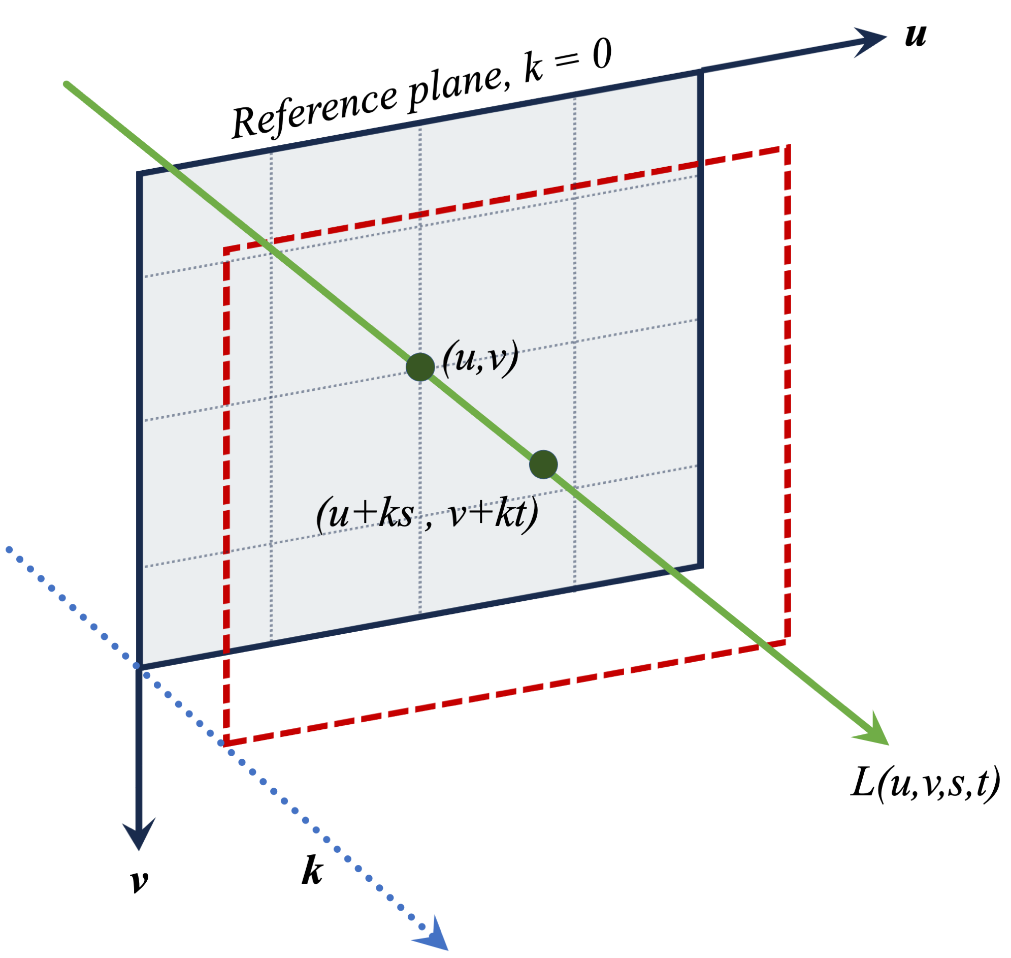
(a)

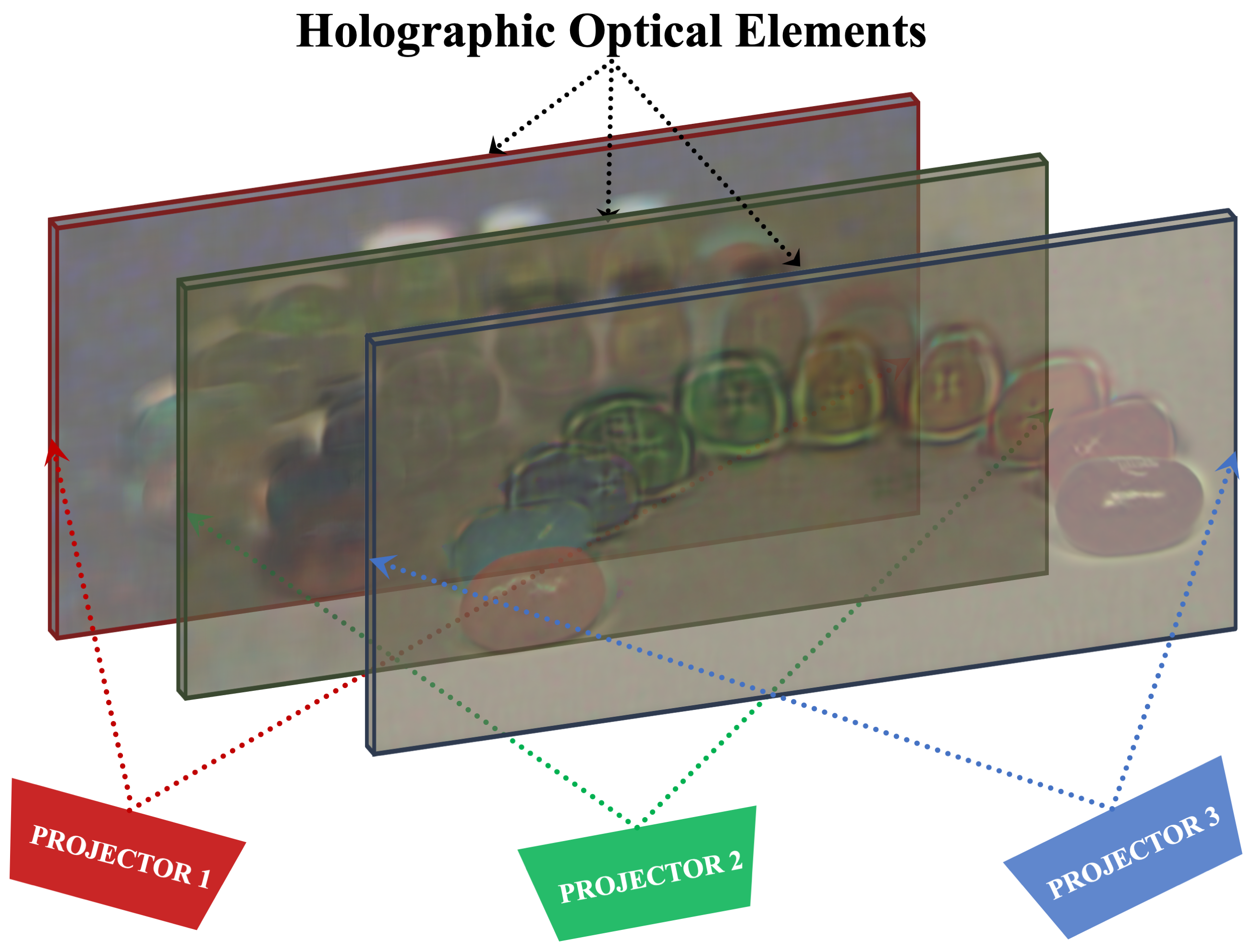
(b)

Figure 1: $(a)$ Simplified 4D light field, $(b)$ Structure of additive layered light-field display.

Researchers have employed various techniques to develop glasses-free multi-view/light-field displays. These methods include the use of parallax barriers Ives (1903); Isono et al. (1993); Sakamoto and Morii (2006); Peterka et al. (2008), specially designed lenses such as lenticular screens or integral photography lenses Lippmann (1908); Börner (1993); McCormick (1995), stacked layers Wetzstein et al. (2012); Takahashi et al. (2018) and layered display Maruyama et al. (2020); Lee et al. (2016). Extended depth of field, wider field of view, and thin form factor are desirable characteristics defining an excellent light field display. Therefore, incorporating these features is necessary to ensure the display produces a clear, accurate light field that provides users with a realistic and engaging viewing experience.

Augmented reality (AR) technology allows digital information to be overlaid in the real world, creating a composite view. Flat displays in current AR wearables generate conflicting depth information. It lacks monocular depth cues, resulting in three significant visual conflicts: vergence accommodation conflict, focal rivalry and ocular parallax Kramida (2015); Konrad et al. (2020). The light field display can be integrated into AR wearables by overlaying 3D digital information onto the real world without visual conflicts Sluka et al. (2021).

We illustrate the conventional structure of an additive layered display in Fig. 1(b). This display uses holographic optical elements (HOEs) as transparent layers to diffuse projected images from projectors, creating separate 2D light fields. The combined light rays from each layer pass through different pixel combinations based on viewing angles, resulting in a 4D light field. Additive light field displays do not suffer from the moiré effect, a visual artefact that decreases brightness and colour accuracy in LCD-based compressive displays. The transparent holographic optical elements (HOEs) make additive layered displays well-suited for augmented reality (AR) applications. This technology offers users a highly immersive and interactive way of experiencing digital content, allowing them to engage with virtual objects more naturally and intuitively.

Plenoptic data contains detailed information about the direction and intensity of light rays in a scene, resulting in a large amount of data with spatial, angular, and temporal redundancies. It is essential to consider these inherent correlations to create an effective compressive content delivery pipeline via multi-layered based tensor displays. Many currently available methods for encoding light field data are unsuitable for multi-layered display technologies. Various encoding algorithms extract sub-aperture images (SAIs) and create a pseudo video sequence in light field data compression Liu et al. (2016); Li et al. (2017). Commonly used video encoders like HEVC Sullivan et al. (2012) or MV-HEVC Hannuksela et al. (2015) are employed for inter and intra-frame hybrid prediction. However, current view estimation-based coding methods cannot remove redundancies among adjacent SAIs and are limited to local or frame units of the encoder Senoh et al. (2018); Huang et al. (2018); Hériard-Dubreuil et al. (2019). Learning-based view-synthesis techniques require a vast and diverse dataset to achieve better compression Bakir et al. (2018); Wang et al. (2019); Jia et al. (2018); Liu et al. (2021). Some techniques use the low-rank structure in light field data based on disparity models, while others use light field structure/geometry to compress at low bitrates Vagharshakyan et al. (2017); Ahmad et al. (2020); Chen et al. (2020). However, these methods are still are not suitable for layer pattern encoding for additive layered displays.

This paper introduces a novel method for encoding layer patterns of additive light field displays in a scalable and efficient manner. The proposed scheme involves using a convolutional neural network (CNN) to obtain the optimised layer pattern for the display. Our aim of achieving a scalable framework led us to convert the layers into their weighted binary image form. The binary images and their appropriate weight can reconstruct the layers with minimal distortion, and the reconstruction accuracy improves as more binary images are considered. Moreover, the divide-and-conquer strategy inherent in the scalable structure significantly reduces computational complexity. The weighted binary image is highly compressible, as the pixel values take either $0$ or $1$ to represent black and white pixels, respectively. We employ a powerful generative model to exploit the inherent strong correlations in binary images. The deep autoencoder model learns low dimensional codes that reduce the dimensionality of data. Our deep architecture uses multiple stacks of Restricted Boltzmann Machines (RBM) Teh and Hinton (2000), which form the Deep Belief Network (DBN) Hinton and Salakhutdinov (2006). In DBN, the hidden layer (learned features) of an RBM feeds to the visible layer on the next RBM on the stack. Finally, the widely adopted HEVC (HM 17.0) Sullivan et al. (2012) standard video codec is employed on the latent code to compress further and eliminate intrinsic redundancies in latent data blocks, generating a bitstream compatible with most decoder devices. Our tests with both real-world and synthetic light field data demonstrate highly competitive outcomes. The principal contributions introduced in the proposed light field encoding technique can be summarized as:

• The paper presents a new light field coding method for additive layered displays, which effectively eliminates spatial, temporal, angular, and non-linear redundancies between adjacent sub-aperture images in a single integrated framework. The first component of the proposed approach operates to eliminate both intra-view and inter-view redundancies, leading to the derivation of distinct layer patterns. The second block effectively mitigates highly correlated non-linear redundancies among the patterns. Overall, the proposed framework represents a highly efficient and comprehensive solution for light field coding.

• The integrated and versatile framework of weighted binary images and deep belief networks (DBN) facilitates scalability in light field reconstruction. The number of levels utilized in the proposed approach plays a critical role in determining the reconstruction quality, whereby progressively increasing levels correspond to improved accuracy. The proposed framework thus represents a powerful solution for high-quality reconstruction with support for multiple bitrates, all within a single integrated pipeline.

• In the proposed scheme, hybrid convolutional neural networks (CNN) and deep belief networks (DBN) offer adaptability across multiple bitrates, providing a highly flexible solution for light field coding. This scheme differs from traditional light field coding approaches that typically support fixed bitrate during compression. Furthermore, the proposed approach employs optimised layer patterns to process the light field data efficiently, eliminating the need to process the entire data set.

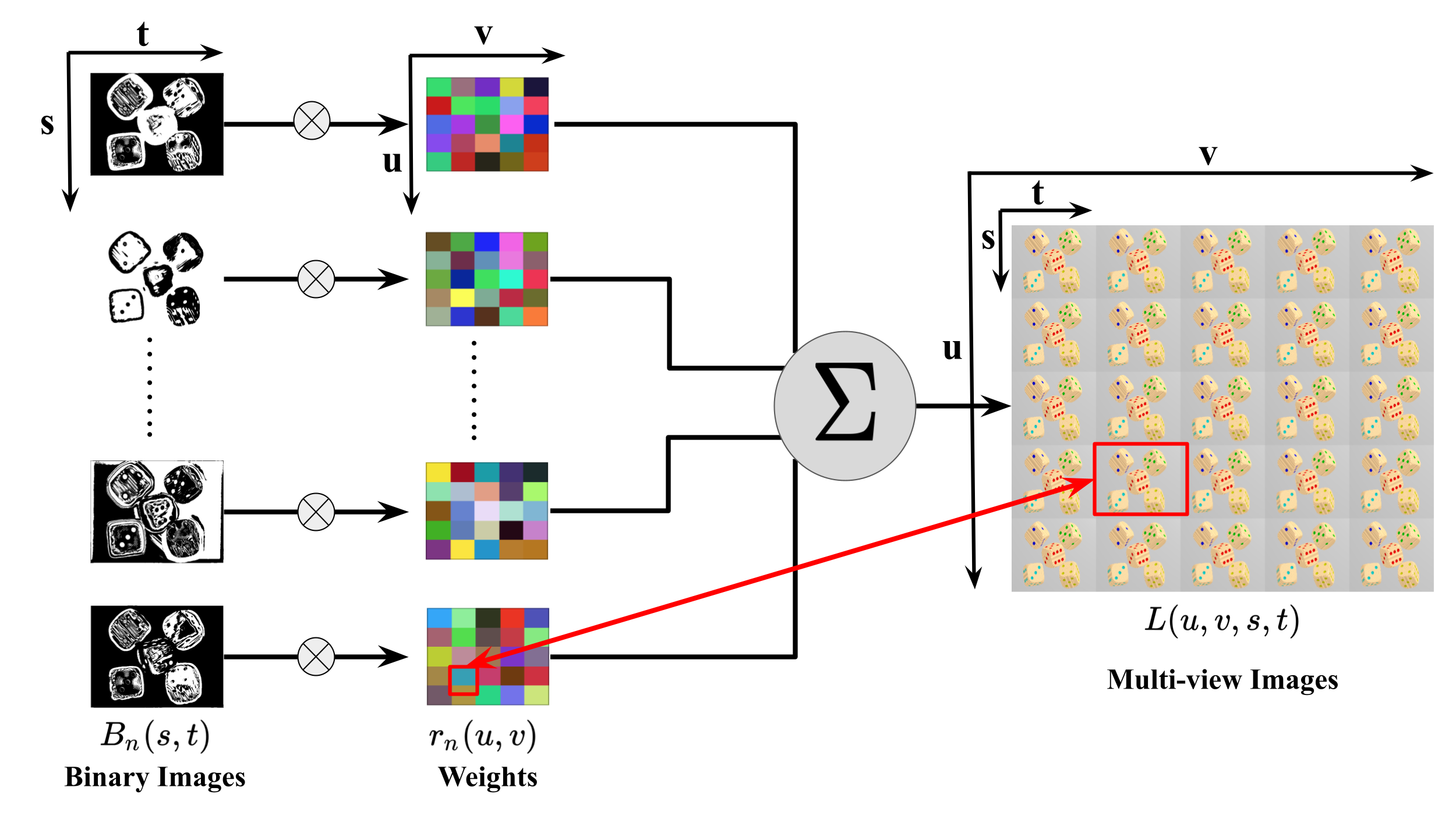
(a)

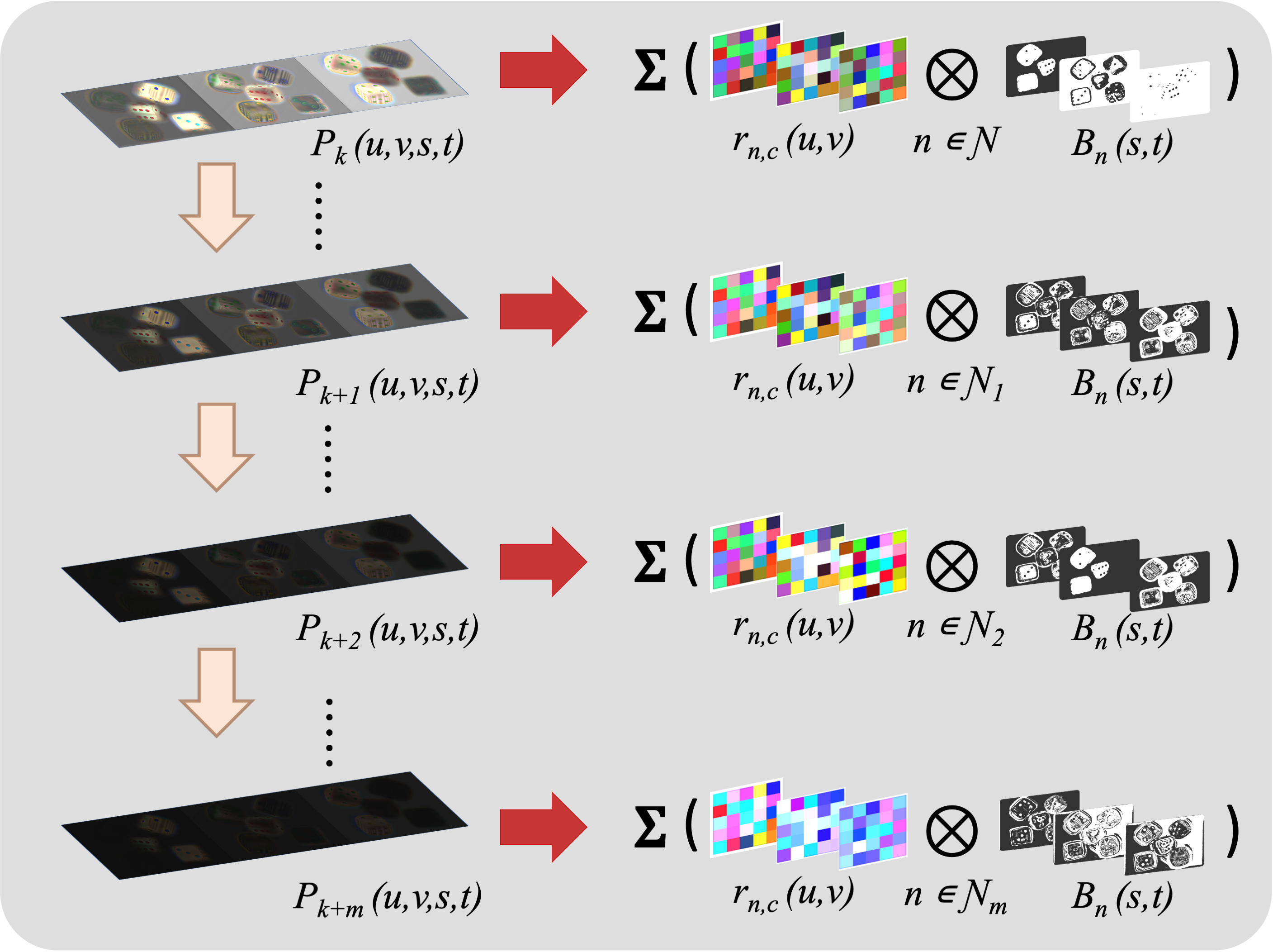
(b)

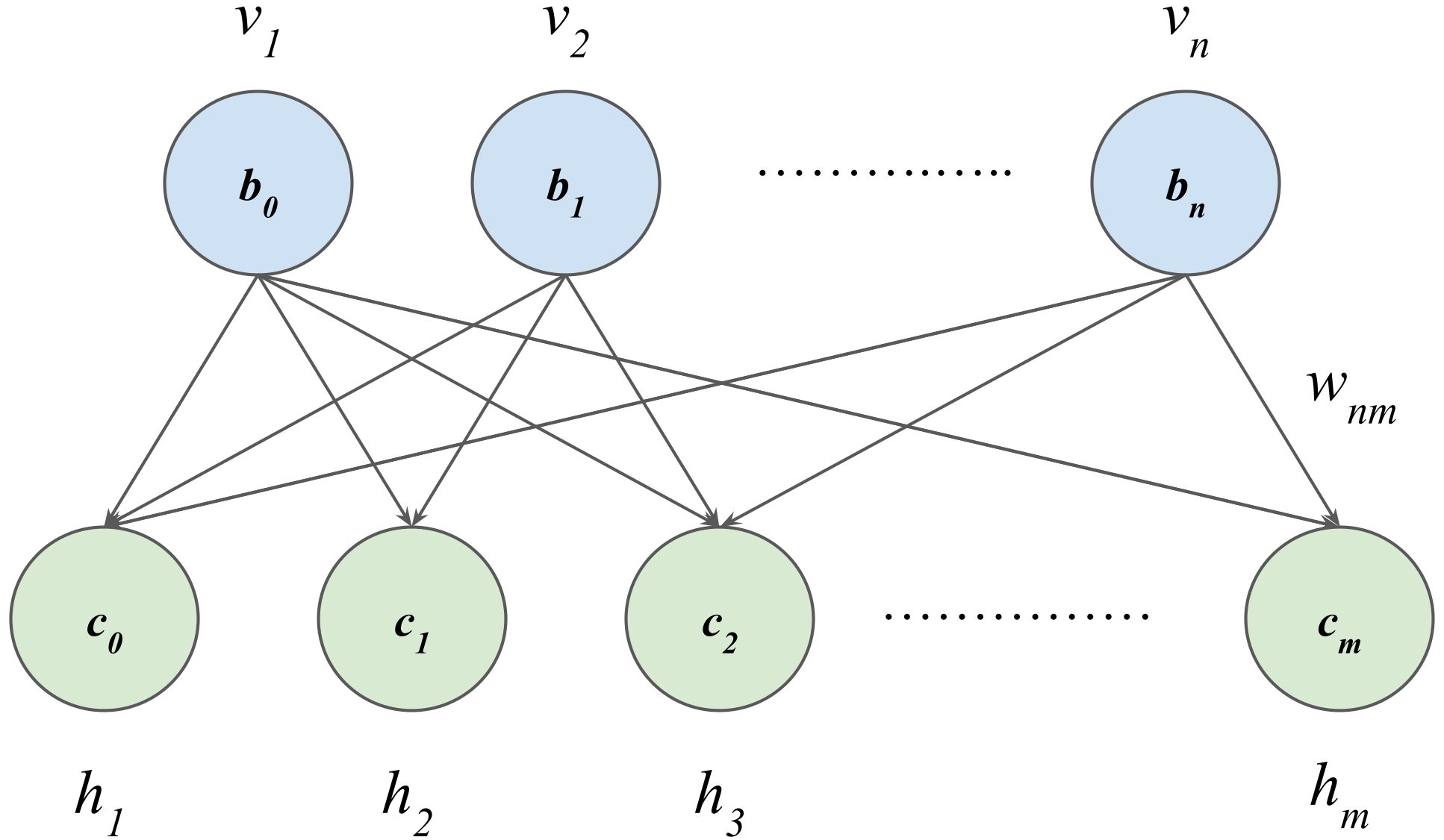
(c)

Figure 2: $(a)$ Compressed light field representation using binary images $B_{n}(s,t)$ and weights $r_{n}(u,v)$ $(b)$ Workflow of scalable encoding process $(c)$ Structure of restricted boltzmann machine network.

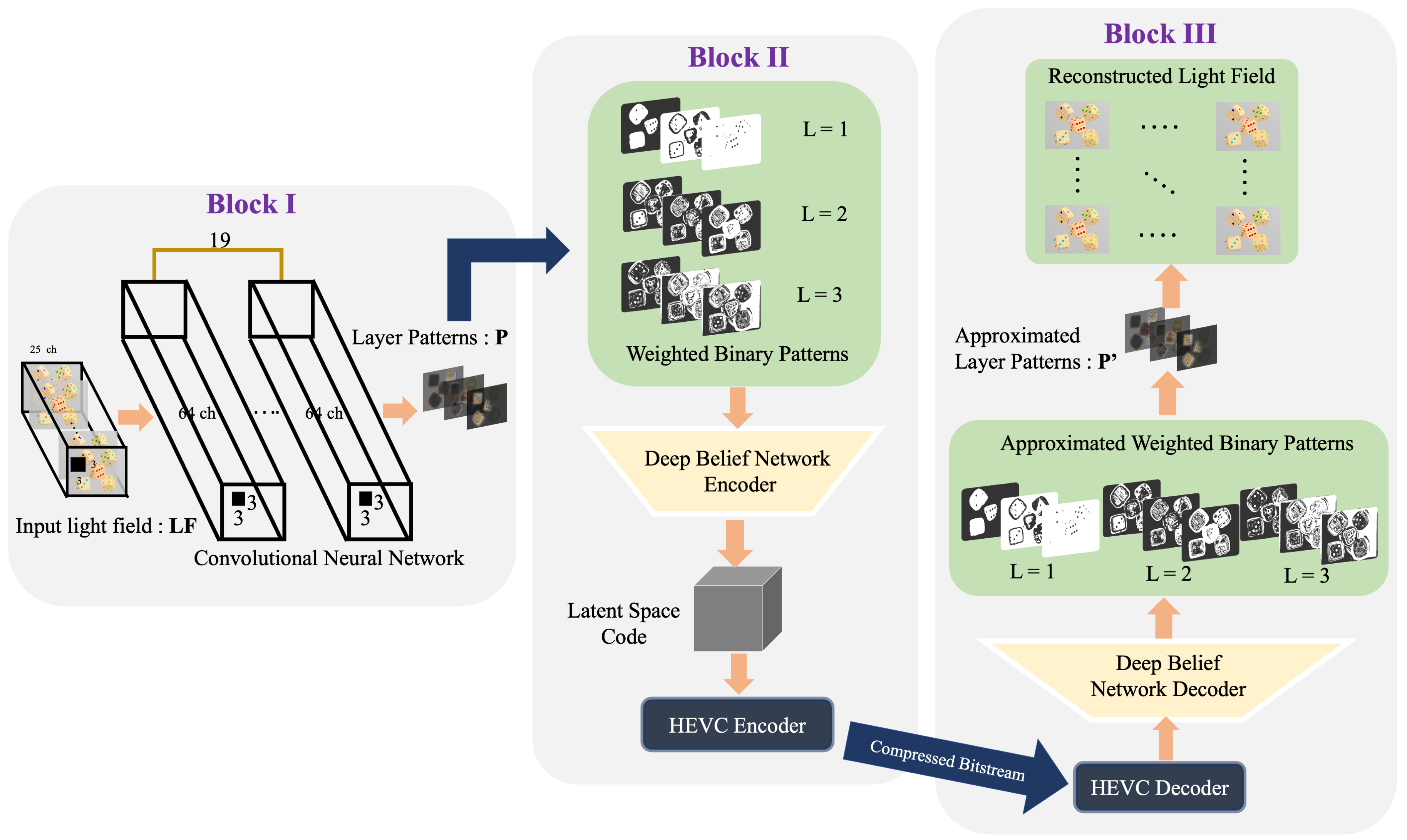
Figure 3: Complete workflow of proposed coding scheme.

2 Proposed Coding Scheme for Multi-Layered Displays

Our representation and coding pipeline consists of three blocks. The complete workflow is illustrated in Fig. 3. BLOCK 1 (Fig. 3) transforms the entire light field into additive layer patterns using a CNN-based approach. A more efficient and scalable representation of the layer pattern is achieved through a DBN and HEVC encoding in BLOCK II. The light field reconstruction from approximated layers is performed in BLOCK III. The implementation steps of the proposed methodology is described in Algorithm  1.

The multidimensional plenoptic function represents the amount of light travelling through each point in space in each direction. We adopt an angle + plane parameterization with a reference plane at $k=0$ as shown in Fig. 1(a). The 7-D function, $L(x,y,z,\theta,\phi,\lambda,t)$ is constructed by measuring light ray at every potential incidence $(\theta,\phi)$, wavelength $\lambda$, and time $t$. We parameterised light ray by the point of intersection with the reference plane $[(u,v)]$ and the outgoing direction with respect to the z-axis $[(\theta,\phi)]$. Hence, it is simplified into a 4-D function $L(u,v,s,t)$, where $s=\tan(\theta)$ and $t=\tan(\phi)$. In the light field model, $st$ is considered the plane for a set of cameras having $uv$ as their focal plane. Hence, $st$ and $uv$ are called the angular and spatial resolution, respectively.

2.1 Additive Layer Pattern Generation

The main objective of an autostereoscopic 3D display is to support simultaneous viewing from multiple perspectives without compromising the resolution of each viewpoint. An example of such transparent tensor display is the “additive layered display” illustrated in Fig. 1(b). The display consists of transparent HOE projection layers which diffuse images from projectors generating independent 2D light fields. The resulting 2D light fields are merged by addition operation into a 4D light field, providing motion parallax according to the viewing position. The emitting light ray is formulated as shown in Equation 1.

$$L_{add}(u,v,s,t)=\sum_{k\in Z}P_{k}(u+ks,v+kt)$$ (1)

where, $P_{k}(u,v)$ denotes transmittance of the layer located at $k\in Z$. We assumed that there are three layers in the light field display located at $k={-1,0,1}$.

A CNN-based network optimises additive layers to display the target 3-D scene as shown in Block I of Fig. 3. The network consists of sequentially stacked 20 2D convolutional layers. The spatial size of the tensors is constant, while only the number of channels is varied throughout the network. The tensors L and $\mathbf{L_{add}}$ have 25 channels each corresponding to the $5\times 5$ viewpoints. While tensor P has three channels each for the layers in the display, the intermediate feature maps have 64 channels. The mapping function of the optimisation process is expressed as

$$f:L\to P$$ (2)

where, $L$ denotes the tensor with all pixels of $L(u,v,s,t)$ for all $(u,v)$ and $P$ represents the tensor with all pixels of $P_{k}(s,t)$ for all $k\in Z$. The mapping from layer patterns back to light field can be expressed as

$$g:P\to L_{add}$$ (3)

where, $L_{add}$ denotes all light rays in $L_{add}(u,v,s,t)$. The CNN is constructed such that it corresponds to the composite mapping of $g\circ f$ minimising squared loss error as expressed in  (4).

$$\underset{f}{argmin}=\left\|L-L_{add}\right\|^{2}$$ (4)

2.2 Scalable Coding with Weighted Binary Images

The obtained layer patterns are transformed into a weighted binary representation, where binary images with defined weights can approximate the layers Komatsu et al. (2018). There are only two possible intensity values (black and white) in binary images. They are notably helpful for segmentation and thresholding applications in image processing. The compressed representation (Fig. 2(a)) of layer patterns is possible using weighted binary images. The binary images $B_{n}$ and their corresponding weights of ‘$c$’ channel, $r_{n,c}$ can optimally approximate the layers pattern $P_{k}$ as formulated in  (5). The binary image captures common features for all viewpoints and the pixel-independent weights contain the differences between the layers.

$$P_{k}(u,v,s,t)\simeq\sum_{n=1}^{N}B_{n}(s,t)r_{n,c}(u,v)$$ (5)

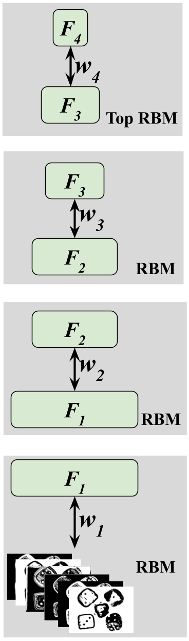
(a)

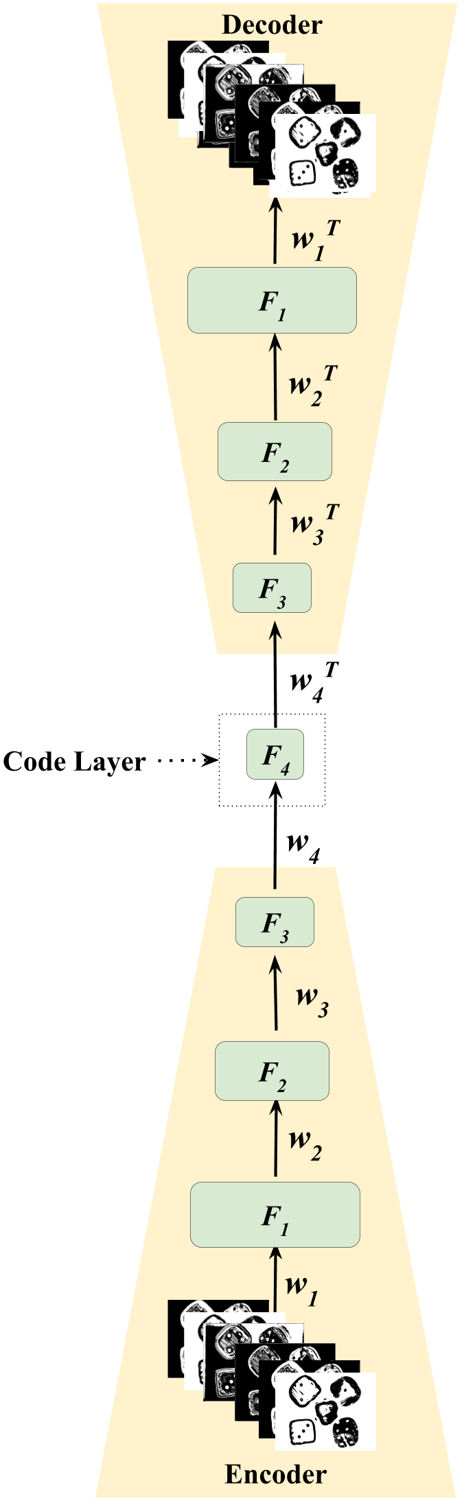
(b)

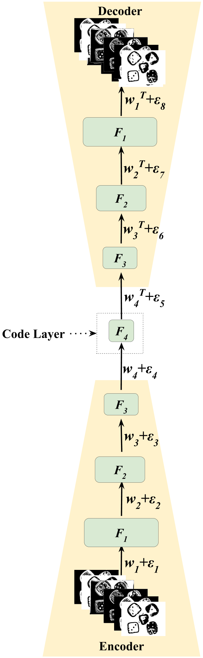
(c)

Figure 4: Workflow of deep auto-encoder with RBM pretraining.$(a)$ Pre-training of RBM weights $(b)$ Unrolling of stacked RBMs $(c)$ Fine-tuning of the unrolled stacked RBMs network.

In order to obtain the compressed binary representation, it is necessary to solve the optimisation problem defined in  (6)

$$\begin{split}\underset{B_{n}(u,v),r_{n,c}(u,v)}{argmin}\sum_{u,v,s,t}\left|P_{k}(u,v,s,t)-\sum_{n=1}^{N}B_{n}(s,t)r_{n,c}(u,v)\right|^{2}\end{split}$$ (6)

The pipeline adopts two alternate approaches for the two unknowns, $B_{n}$ and $r_{n,c}$. It initialises the binary images $B_{n}$ and repeats the following two steps until convergence.

1. Optimise the weights $r_{n,c}(u,v)$ keeping binary images $B_{n}(s,t)$ fixed. This step involves solving standard least squares problems.

2. Optimise binary images $B_{n}(s,t)$ keeping the weights $r_{n,c}(u,v)$ fixed. The individual pixels $(s,t)$ are solved using binary combinatorial optimisation technique which is a NP-Hard problem Toth (2000).

Since combinatorial optimisation employs exhaustive search, the introduction of scalability in the framework plays a vital role in drastically increasing the speed and reducing computational complexity. For scalable coding (Fig. 2(b)), the divide and conquer method is adopted. The $N$ number of layer patterns are divided into $M$ groups, which correspond to the number of levels for scalability. Firstly, $M$ sets of integers are defined such that $\left\{N_{1},...,N_{m}\right\}$ satisfy $N_{i}\cap N_{j}=\phi$ for $i\neq j$ and $\bigcup_{m=1...M}\ N_{m}=\left\{1,..,N\right\}$. $N_{m}$ denotes the binary images for the $m^{th}$ level and $\sum_{m}\left|N_{m}\right|=N$. For original $N$ bit binary combinatorial optimisation, the computational complexity is $\mathcal{O}(2^{N})$. The complexity is reduced to $\mathcal{O}(\sum_{m}2^{\left|\mathscr{N}_{m}\right|})$ when divided into $M$ sublevels. The approximation accuracy of the encoding process improves progressively as the number of levels increases. The target layer patterns $P_{k+1}(u,v,s,t)$ is set to original layer pattern $P_{k}(u,v,s,t)$ in the first level. The best approximation of the layer patterns is evaluated at each level using the binary images $B_{n}(s,t)$ along with their corresponding weights $r_{n,c}(u,v)$ and are optimised as shown in (7).

$$\begin{split}\underset{B_{n}(u,v),r_{n,c}(u,v)}{argmin}\sum_{u,v,s,t}\left|P_{k+M}(u,v,s,t)-\sum_{n\in N_{M}}B_{n}(s,t)r_{n,c}(u,v)\right|^{2}\end{split}$$ (7)

The calculation of target layer pattern for the next level using residual from the first layer is shown in (8)

$$\begin{split}P_{k+1}(u,v,s,t)=P_{k}(u,v,s,t)-\sum_{n\in N_{M}}B_{n}(s,t)r_{n,c}(u,v)\end{split}$$ (8)

The steps in (7) and (8) are repeated to the $M^{th}$ level. Hence, a scalable representations with $M$ levels is realised as

$$P_{k}(u,v,s,t)\simeq\sum_{m=1}^{M}\sum_{n\in N_{m}}B_{n}(s,t)r_{n,c}(u,v)$$ (9)

As the level progresses, the residual (10) exhibits a monotonic decrease, indicating that less information is available for the higher level. This decrease is accompanied by a progressive improvement in the accuracy of the decoded layer patterns, which is beneficial in various real-world scenarios, such as adaptive rate control and flexible user adaptability. The progressive improvement in accuracy is a direct result of the increasing number of levels, which allows for the incorporation of finer details in the reconstructed image. These findings suggest that the proposed method is well-suited for a wide range of applications that require high-quality reconstructed images with adaptive resolution.

$$\left|P_{k+1}(u,v,s,t)\right|\leq\left|P_{k}(u,v,s,t)\right|$$ (10)

2.3 Deep Belief Network

Input: Input light field $\mathbfit{L(u,v,s,t)}$

Output: Non-linear low dimensional code, $\mathbfit{NLD}$

1

2Initialize $\mathbfit{P_{k}(u+ks,v+kt)}$ where $u$ and $v$ are limited to the range $[-2,2]$ and $Z=\{-1,\ 0,\ +1\}$

3repeat

4       for $k\in Z$ do

5             $\mathit{arg\ \underset{P_{k}|k\in Z}{min}}\sum\limits_{u,v,s,t}\left\|L(u,v,s,t)-\sum\limits_{k\in Z}P_{k}(u+ks,v+kt))\right\|^{2}$

6      

7until optimisation problem is solved

8Initialise first level ($m=1$) of binary weighted pattern $\mathbfit{W_{1}(u,v,s,t)\Leftarrow P_{k}(u,v,s,t)}$

9for  $m=1\ to\ M$ do

10       Obtain $\mathbfit{B_{n}(s,t)}$, $\mathbfit{r_{n,c}(u,v)}$ where $n\in\mathscr{N}_{m}$ by solving $\mathit{arg\ \underset{B_{n}(s,t)r_{n,c}(u,v)}{min}}\sum\limits_{u,v,s,t}\left\|P_{k}(u,v,s,t)-\sum\limits_{n\in\mathscr{N}_{m}}B_{n}(s,t)r_{n,c}(u,v)\right\|^{2}$

11       Carry over the residual as

12       ${W_{m+1}(u,v,s,t)}={W_{m}(u,v,s,t)}-{\sum\limits_{n\in\mathscr{N}_{m}}B_{n}(s,t)r_{n,c}(u,v)}$

13       $m\Leftarrow m+1$

14Dimensionality reduction of $\mathbfit{B_{n}(s,t)}$ for $\mathbfit{n\in\mathscr{N}_{m}}$

15 for n = 1 to $\mathscr{N}_{m}$ do

16       $\mathbfit{NLD}\leftarrow\mathbfit{Algorithm\ 2}\ (\mathbfit{B_{n}(s,t)})$

Algorithm 1 Proposed scalable encoding coding scheme

The binary layer patterns $B_{n}(s,t)$ and their weights $r_{n,c}(u,v)$ provides an approximate representation of the actual layer patterns. Algorithms such as auto-encoder encode the input data into a much smaller dimensional representation and store latent information about the input data distribution. An RBM is a two-layered stochastic network with visible and hidden layers(Fig. 2(c)). It is a probabilistic model composed of weights and biases. The structure consists of $``n"$ visible units $\mathbf{v=(v_{1},..,v_{n})}$ representing the observed data and $``m"$ hidden units $\mathbf{h=(h_{1},..,h_{m})}$ to illustrate the dependencies in the observed data. There is no interconnection among the nodes in each layer to ensure their mutual independence. In binary RBMs, the random variables take the value $(v,h)\in\left\{0,1\right\}^{m+n}$. The hidden and visible variable vectors, $\mathbf{v}$ and $\mathbf{h}$ can be represented by their joint probability density as

$$p(\mathbf{v},\mathbf{h})=e^{-E(\mathbf{v},\mathbf{h})}\bigg{/}\int\int_{\mathbf{v},\mathbf{h}}e^{-E(\mathbf{v},\mathbf{h})}$$ (11)

where $E(\mathbf{v},\mathbf{h})$ is the associated energy function. Since the input data is binary-value, we apply binary-binary energy function Shang et al. (2014) as described in (12).

$$E(\mathbf{v},\mathbf{h})=-\sum_{i=1}^{m}\sum_{j=1}^{n}w_{ij}h_{i}v_{j}-\sum_{j=1}^{n}b_{j}v_{j}-\sum_{i=1}^{m}c_{i}h_{i}$$ (12)

where, $w_{ij}$ is the weight associated with the nodes $v_{i}$ and $h_{j}$. The bias terms for $j^{th}$ visible and $i^{th}$ hidden node are $b_{j}$ and $c_{i}$ respectively. The network assigns a probability to every possible image using the energy function. Adjusting the weights and biases to reduce the energy of a training image, increases the probability of that image. The weights are adjusted as shown in (13).

$$\Delta w_{ij}=\varepsilon(\left\langle v_{i}h_{j}\right\rangle_{data}-\left\langle v_{i}h_{j}\right\rangle_{recon})$$ (13)

where $\varepsilon$ is the learning rate, $\left\langle v_{i}h_{j}\right\rangle_{data}$ and $\left\langle v_{i}h_{j}\right\rangle_{recon}$ are the fraction of times pixel $i$ and feature $j$ are on together when driven by data and reconstruction data respectively.

Input: $\mathbfit{DBN}$, training set $\mathbfit{X}$

Output: Pre-trained $\mathbfit{DBN}$

1 Initialize network parameters $\mathbfit{w,b}$

2 $\mathbfit{Input}\leftarrow\mathbfit{X}$

3 for  all RBM in DBN do

4       for  epoch = 1 to e do

5             for  k = 1 to floor($N_{sample}/N_{batch\ size}$) do

6                   $\mathbfit{B}\leftarrow\ batch\ from\ \mathbfit{Input}$

7                  $\mathbfit{\Delta{w},\Delta{b}}\leftarrow k\ Contrastive\ Divergence$

8                  $\mathbfit{w\leftarrow w+r.\Delta{w}}$

9                   $\mathbfit{b\leftarrow b+r.\Delta{b}}$

10                  

11            

12      $\mathbfit{X\leftarrow Input\times w+b}$

Algorithm 2 Layer-by-layer pre-training of DBN

A single layer of binary RBM is not the most effective technique to model the input data structure. A deep belief network (DBN) is a stack of RBMs (Fig. 4) where the hidden layer of one RBM is the visible layer of next RBM. Stacking individual RBMs to form a chain drastically improves the performance, similar to a multi-layer perceptron outperforming a single perceptron. In DBN, the training procedure happens in two stages: unsupervised layer-by-layer pre-training and fine-tuning. During pre-training, we employ a layer-wise greedy technique(Fig. 4(a)). Once the training of previous RBM completes, its hidden layer is the visible layer for the next RBM. Likewise, the training of all RBMs occur one after another until the last RBM is trained. After pretraining completion, the model unfolds to form a deep auto-encoder network initialised with the pre-trained weights (Fig. 4(b)). The training of each RBM maximises the probability of its input data exploiting contrastive divergence (CD) Hinton (2002) algorithm to update the network parameters. Each feature layer detects the strong and high-order correlations between the units in the layer beneath it. The pre-trained weights are fine-tuned (Fig. 4(c)), minimising the cost function. We implement the back-propagation algorithm to update the whole network’s parameters, progressively passing the error from the last layer to the bottom input layer. The pipeline achieves latent space representation of the weighted binary data using a DBN. The number of features extractors $F_{1}$, $F_{2}$, $F_{3}$ and $F_{4}$ in each layers are varied according to the requirement of input data such that $F_{2}>F_{3}>F_{4}$ and $F_{2}>F_{1}$ . The code layer with $F_{4}$ features is the latent space representation of the input data. The encoder and decoder network share a symmetrical structure and number of features in each layer. The latent code are encoded using standard video codec HEVC (HM 17.0). The implementation details and experimental results are analysed in the later sections.

3 Experiments

To evaluate the performance of the proposed scheme, we perform experiments on both real and synthetic light fields. We choose $Amethyst$, $Bunny$, and $JellyBeans$ light fields from the Stanford Light Field Archive Vaish and Adams (2008) as well as the $Boxes$ Honauer et al. (2017), $Dice$, $Dragon$ and $Bunnies$ Marwah et al. (2013) synthetic light fields. As illustrated in BLOCK I of Fig. 3, we take the complete light field data as input to generate an optimized additive layer patterns. The additive layer patterns are represented as scalable weighted binary maps, which are compressed using Deep Belief Networks in BLOCK II with variable bitrate support. The compressed data is further encoded using HEVC to generate an encoded bitstream, which was subsequently decoded and reconstructed back into the complete light field in BLOCK III.

3.1 Implementation Details

The implementation of the proposed scheme is done on a single system with 9th Gen i7, 32 GB RAM, RTX 2080 8 GB Graphics with Ubuntu 22.04 operating system. We implement the sequentially stacked network of 20 2-D convolutional layers in BLOCK I (Fig. 3) using Chainer (version 7.7.0), a Python-based framework. The optimisation problem defined in Equation (4) computes the mean square difference between the original and reconstructed light field, which is obtained from additive layers optimised by the CNN. These layer patterns are represented as weighted binary images, which can optimally approximate them. We perform experiments considering various scalable layers and number of binary images as depicted Fig. 2(b). As we incorporate more layers into the encoding process, the reconstruction quality increases progressively. This validates the progressive increment of reconstruction quality as more information is utilised as shown in Fig. S12. Here, we introduce rate scalability aspect in the framework. The DBN encodes weighted binary patterns into a dimensionally reduced representation. The encoder (Fig. 4) has layer size of $F_{1}-F_{2}-F_{3}-F_{4}$ and symmetric decoder layout $F_{4}-F_{5}-F_{6}-F_{7}$, where $F_{1}=F_{7},\ F_{2}=F_{6}\ \text{and}\ F_{3}=F_{5}$. The training sample for the network is a set of $64\times 64$ 2-D image blocks derived from the exact locations in all image views of the sample light field. The sample patch of $64\times 64$ pixels is collected from the training data $32$ pixels apart in horizontal and vertical directions, discarding the patches with nearly uniform intensities. The training samples are collected from several light field datasets Vaish and Adams (2008); Marwah et al. (2013); Honauer et al. (2017). The training data differs from the test data. The testing is done on Amethyst, Boxes, Bunny, Dice, DragonsAndBunnies and Jellybeans light field dataset having $5\times 5$ viewpoints. While training, eight sets were considered, each consisting of 64000 samples and trained for 30 epochs taking around 5 hours for each sample set. The initial weights are small random values procured from a normal distribution having zero mean and a standard deviation of 0.1. We adjust the weights with a learning rate of 0.1 after each mini-batch (Equation 12). To encourage stability and prevent overfitting, we use a regularization technique involving a combination of additive and penalty terms. Specifically, we add 0.9 times the value of the previous update to each weight, which helped to ensure gradual changes over time. Additionally, we subtract 0.00002 times the weight value from the update, which penalises large weights and encouraged the model to focus on essential features. The latent data from BLOCK II is encoded using HEVC (HM 17.0), generating an encoded bit-stream that can be scaled to reconstruct at any desired bitrate (quality). The performance of our proposed Scalable and Non-Scalable coding schemes are compared with standard video codec, HEVC (HM 17.0) Sullivan et al. (2012) as illustrated in Fig. 11. We covered the range of HEVC (main10) quantization parameters, QP $0$, $4$, $8$, $12$, $16$, $20$, $24$, $28$, $32$, $36$, $40$, $44$, $48$, $51$ to test the performance at both high and low bitrate cases. In Table 1, an objective assessment to compare bitrate reduction of the proposed scheme (Scalable and Non-Scalable) with respect to HEVC codec is done using the Bjontegaard Bjontegaard (2001) metric. The more negative value of BD-Rate, the more gain in bitrate is achieved by the proposed scheme and similarly for BD-PSNR. Subsequently, the decoder of DBN decompresses the bitstream from BLOCK II to regenerate the approximated layer patterns and then transform them into the whole light field. In Fig. S5, S6, S7, S8, S9, S10, we illustrate the reconstructed layers using four scalable levels with four images per level along with the original layers.

3.2 Comparative Analysis

Based on our experimental results, we can make some significant conclusions. Firstly, our proposed coding scheme demonstrates remarkable flexibility in producing high-quality reconstructions at higher bitrates. However, the conventional codecs do not support such scenarios. Additionally, it is able to deliver quality on par compared to HEVC even at lower bitrates, which is impressive. To achieve scalability in the pipeline, we implement a multi-level coding approach using the divide-and-conquer method, reducing computational complexity. Furthermore, as illustrated in Fig. S12, the decoding accuracy improves progressively as we incorporate more binary images, enhancing the overall efficiency of the system.

4 Conclusion

We introduce an efficient representation and scalable coding scheme of a light field for layered light-field displays based on a DBN. Existing light field compression algorithms do not utilise the similarities between the views of a light field to compress them effectively. The proposed scheme exploits the additive layers’ spatial, temporal, angular and other non-linear intrinsic redundancies. The proposed hybrid CNN and DBN model generates the optimised transmittance patterns, while learning and preserving only the essential features in a latent code form. Weighted binary images represent the optimised layer patterns in the intermediate stage, where we introduce scalability in the framework. Further encoding with HEVC generates a rate scalable bitstream which supports any desired bitrate (quality) decoding. The decoding performance progressively improves as we use more encoded information in the reconstruction process. As a result, our proposed scheme achieves the goal of covering a wide range of bitrates within a single trained model without compromising the quality of the reconstruction. Experiments with benchmark light field datasets produce competitive results. Since additive layered display is a transparent autostereoscopic display, it can be easily adopted to AR applications. Unlike other light field display, the HOE layers in additive display do not suffer from moiré effect. We plan to test our scheme with physical light field display hardware in the future. Furthermore, we would like to improve the proposed scheme to deliver 3D content on devices with limited hardware resources.

5 Supplementary Material:

Table 1: The percentage rate savings based on Bjontegaard metric for the proposed compression scheme with respect to HEVC (HM 17.0) on Amethyst, Boxes, Bunny, Dice, DragonAndBunnies and Jellybeans light fields.

	Amethyst								Boxes
	Non-Scalable N = 1		Scalable N = 2		Scalable N = 3		Scalable N = 4		Non-Scalable N = 1		Scalable N = 2		Scalable N = 3		Scalable N = 4
QP	BD-Rate	BD-PSNR	BD-Rate	BD-PSNR	BD-Rate	BD-PSNR	BD-Rate	BD-PSNR	BD-Rate	BD-PSNR	BD-Rate	BD-PSNR	BD-Rate	BD-PSNR	BD-Rate	BD-PSNR
0	-98.8690	57.6900	-55.7210	-8.0804	-61.2000	-7.4733	-24.1800	-15.2940	-41.8959	-11.8468	198.1354	-33.6725	169.2788	-32.8233	225.0941	-35.1330
4	-98.6660	47.7800	-64.4650	-13.8590	-70.9230	-13.2360	-46.5880	-20.7910	-60.0660	-16.2634	73.3905	-37.8468	57.3914	-36.8934	78.3453	-39.2278
8	-95.3180	23.4260	31.3520	-32.7900	17.1520	-32.3530	116.2800	-39.8830	25.4220	-34.0146	526.7320	-55.7807	483.1239	-54.7671	588.0735	-57.2147
12	-86.5830	12.1360	267.0900	-43.1290	232.8400	-43.0600	528.8800	-50.7920	209.7793	-46.9153	1625.4085	-69.7935	1520.5142	-68.4530	1875.0145	-70.9254
16	-66.8830	4.0749	1095.4000	-51.0790	1053.5000	-51.6410	2135.6000	-59.2240	863.3522	-58.7275	5477.7887	-82.8921	5028.0985	-81.0795	6294.1877	-83.2878
20	-30.0260	0.4346	2155.4000	-53.1150	2173.8000	-53.5410	4320.4000	-60.7000	1883.4621	-66.4779	12072.7062	-91.7540	10746.6098	-88.9064	13314.8035	-90.9410
24	-0.8148	2.5083	2152.0000	-46.1940	1964.9000	-42.6370	3591.6000	-49.1290	1974.4314	-59.1979	11442.4152	-81.5360	8855.1567	-75.0587	9672.0447	-73.5113
28	27.8410	5.0623	1396.0000	-38.8420	1019.7000	-29.7390	1687.2000	-35.8920	937.6225	-43.6612	3182.6067	-56.3625	2032.0911	-45.8879	1640.0668	-37.7108
32	66.1340	4.5937	890.8700	-34.2510	570.3500	-21.8320	800.0600	-27.5280	356.6148	-26.4650	587.8523	-25.4563	384.0154	-16.0203	235.1648	-2.1866
36	65.4110	3.0468	512.5400	-25.5620	385.7100	-12.5280	472.1000	-17.6450	223.1411	-27.8435	119.1653	2.3155	65.1886	12.7977	15.0704	36.7899
40	124.9200	6.2937	288.7800	-20.3660	259.5800	-11.6720	289.1500	-16.0210	75.2486	0.0205	39.3248	11.2568	-25.5882	74.0820	-28.8742	15.3309
44	108.3400	-5.2522	219.9400	-30.2000	200.1300	-21.2540	227.6000	-27.0140	72.1109	-14.5280	-7.0705	9.7634	-24.0337	13.7988	-34.9223	16.8794
48	30.8840	13.8740	6.6178	15.8100	23.6090	14.4030	17.8290	14.7260	-22.1333	-2.6566	-28.4868	-1.3393	-28.3266	-1.3673	-29.5321	-1.1023
51	45.1830	-10.1580	22.7340	-8.8224	39.6500	-9.9032	33.6690	-9.5537	-9.7703	-1.1806	-16.3486	0.2101	-16.2866	0.2038	-16.5424	0.2631
	Bunny								Dice
	Non-Scalable N = 1		Scalable N = 2		Scalable N = 3		Scalable N = 4		Non-Scalable N = 1		Scalable N = 2		Scalable N = 3		Scalable N = 4
QP	BD-Rate	BD-PSNR	BD-Rate	BD-PSNR	BD-Rate	BD-PSNR	BD-Rate	BD-PSNR	BD-Rate	BD-PSNR	BD-Rate	BD-PSNR	BD-Rate	BD-PSNR	BD-Rate	BD-PSNR
0	-35.8541	-17.0695	73.0508	-32.3806	160.6051	-39.3341	624.6934	-52.8248	-66.4276	-2.2326	40.6093	-22.5932	130.0192	-28.8897	170.5627	-30.7740
4	-41.8936	-34.0459	40.0770	-49.8663	86.2890	-57.2647	371.3065	-72.0286	-75.9316	-6.9096	-15.6806	-26.5816	22.7096	-32.4988	43.2013	-34.3269
8	175.0928	-54.4521	596.2660	-71.5034	968.0501	-79.8450	2884.9865	-96.0686	-33.4818	-17.8915	158.3820	-36.8031	312.4884	-42.7621	399.1539	-44.3851
12	581.4316	-69.2273	1738.6878	-88.2156	3027.9593	-97.0145	8733.8350	-115.7014	29.9154	-25.3225	422.0706	-44.1848	755.3686	-50.1750	956.5430	-51.6672
16	1744.7020	-81.1327	5404.1429	-101.9941	9187.7433	-111.9698	29726.3101	-132.4633	227.5596	-31.2497	1279.9479	-49.7174	2232.8511	-55.6054	2712.3778	-56.8894
20	3007.3424	-84.3790	9496.2841	-105.7178	17104.4903	-116.9110	59241.9373	-139.1975	440.0170	-31.5654	2349.4750	-49.3073	4050.7552	-54.6757	5005.8425	-55.4995
24	2406.6269	-69.8786	6191.8533	-83.3898	10202.4810	-89.1761	33377.0580	-107.5293	472.3484	-24.1805	2008.4562	-37.2643	3373.7957	-42.3617	3824.9943	-41.7005
28	1181.4572	-53.6379	1707.3778	-52.8878	2611.9269	-58.3495	4573.4586	-60.7393	296.4435	-13.8790	878.9704	-21.6984	1222.9146	-23.3816	1264.8145	-21.9235
32	655.5291	-45.8655	603.1516	-35.9773	1128.7717	-50.2445	1084.3950	-37.4922	144.7853	-4.2159	317.2983	-6.5884	349.4932	-5.1907	326.3524	-2.3271
36	317.9121	-28.6696	186.1383	-12.7256	454.1258	-34.3873	282.1265	-15.3242	45.9910	6.8538	105.9174	4.2912	106.3284	11.0384	100.4304	8.1394
40	143.5400	-18.2187	45.7421	7.3104	209.0109	-27.0753	108.9672	-6.3548	-22.3509	29.1828	12.5711	25.6253	10.0207	27.5119	-11.0958	33.5574
44	125.4312	-42.8964	36.2615	-9.3876	158.8552	-49.7373	38.9808	-2.4908	-62.1477	56.4491	-25.8455	28.2568	-24.2835	28.0635	-41.4466	37.4671
48	-4.4405	-2.4688	-10.8485	-1.1827	-3.5751	-2.5988	-6.8336	-1.9784	-82.2196	22.2027	-75.5257	20.0590	-76.0856	20.2116	-78.8015	21.0589
51	7.4971	-1.0392	2.7308	-0.0387	8.3584	-1.1732	5.3396	-0.5691	-81.5310	22.0370	-75.0849	19.9392	-75.6145	20.0897	-78.4855	21.0813
	DragonAndBunnies								Jellybeans
	Non-Scalable N = 1		Scalable N = 2		Scalable N = 3		Scalable N = 4		Non-Scalable N = 1		Scalable N = 2		Scalable N = 3		Scalable N = 4
QP	BD-Rate	BD-PSNR	BD-Rate	BD-PSNR	BD-Rate	BD-PSNR	BD-Rate	BD-PSNR	BD-Rate	BD-PSNR	BD-Rate	BD-PSNR	BD-Rate	BD-PSNR	BD-Rate	BD-PSNR
0	-85.5156	8.3380	32.0122	-20.2387	72.9238	-23.5259	66.2699	-22.0434	-99.5234	77.9058	-76.7885	-1.9367	-54.4376	-11.1967	125.1849	-29.2147
4	-90.2718	4.0256	-33.2695	-23.2836	-12.0985	-26.6480	-15.2971	-25.0874	-99.3836	55.7624	-82.6403	-15.0227	-69.6617	-23.9664	23.3035	-42.0870
8	-72.5248	-5.6574	131.7141	-31.8302	212.8679	-34.8821	196.4963	-33.1752	-96.7078	33.6512	-1.4889	-32.4229	88.8461	-41.9025	773.3147	-60.4853
12	-48.0885	-12.1782	378.6404	-37.9446	544.6392	-40.9934	514.1859	-38.8798	-91.5477	22.1932	177.6594	-42.7123	455.2631	-52.9002	2623.2910	-72.1530
16	26.6078	-17.6267	1153.7395	-42.8081	1590.5743	-45.7413	1473.7028	-43.0534	-77.3925	13.0968	831.6044	-51.5420	1925.2471	-62.6116	10388.1426	-82.3759
20	110.3281	-18.3464	2105.4681	-41.5987	2906.9074	-44.2775	2430.3875	-40.7478	-48.8109	11.0514	1693.8994	-50.8611	4117.8794	-62.3073	23403.4191	-81.2988
24	123.8702	-10.5361	1665.4596	-31.4250	2048.6159	-30.8901	1559.1508	-27.8501	-38.5762	21.9889	1539.6563	-38.8265	3515.4397	-47.9189	18169.2832	-65.0034
28	56.7639	-0.7447	655.9266	-16.4986	592.6371	-11.8968	451.1796	-8.8809	-54.2492	49.7829	833.6331	-23.1061	1381.1249	-27.2223	4955.1499	-39.5767
32	2.3774	9.0746	172.9573	0.5472	121.8285	6.8847	86.1353	9.6809	-59.9947	66.5945	323.5571	-6.5438	423.1734	-7.6443	677.8773	-6.1105
36	-41.3905	29.7503	7.3674	18.8344	-3.6047	22.8576	-22.2246	29.4171	-65.6308	95.8310	140.9084	12.6884	160.4089	12.6442	6.4096	57.1260
40	-68.2151	57.5858	-51.7591	46.3843	-52.5853	47.4873	-60.6794	58.4989	-58.1097	87.6541	37.2624	30.8651	26.7779	35.6626	-56.4936	138.6558
44	-78.7734	97.5241	-68.6222	62.3341	-66.4932	57.4959	-75.4121	95.2259	-76.5525	22.3631	3.0126	28.2061	2.2206	30.3434	-70.5624	20.7238
48	-85.9083	23.2501	-82.5366	21.8436	-81.8672	21.5962	-83.4843	22.2759	-73.0002	21.4228	-56.0492	17.6430	-55.6653	17.5842	-67.0470	19.8675
51	-83.3053	22.6011	-80.4031	21.4844	-79.9767	21.3327	-80.8549	21.7928	-70.1418	20.4150	-53.9243	16.8270	-53.4734	16.7459	-64.5351	18.9824

(a) Original Layer Pattern

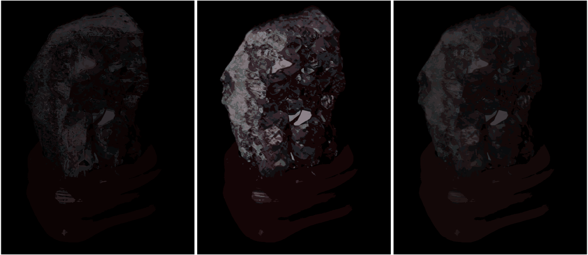
(b) $Level=1$

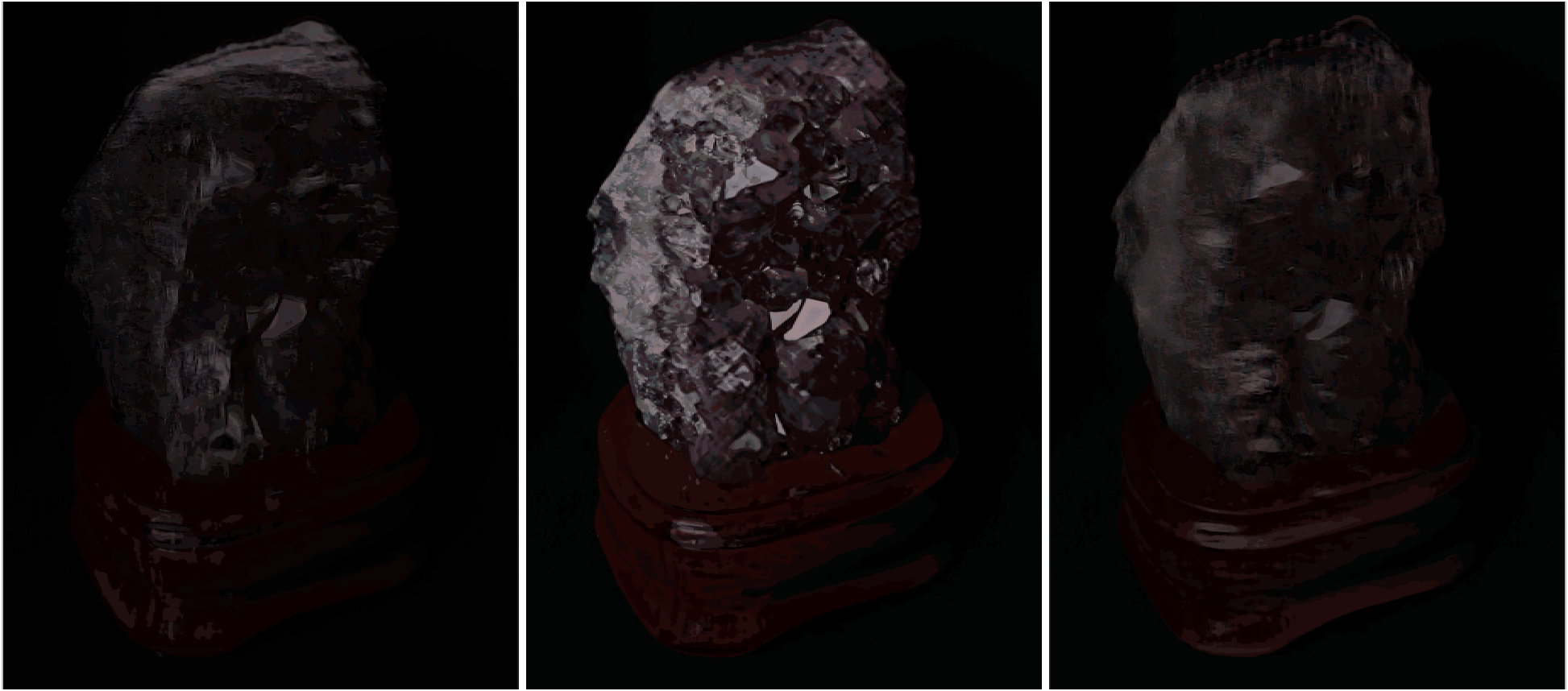
(c) $Level=2$

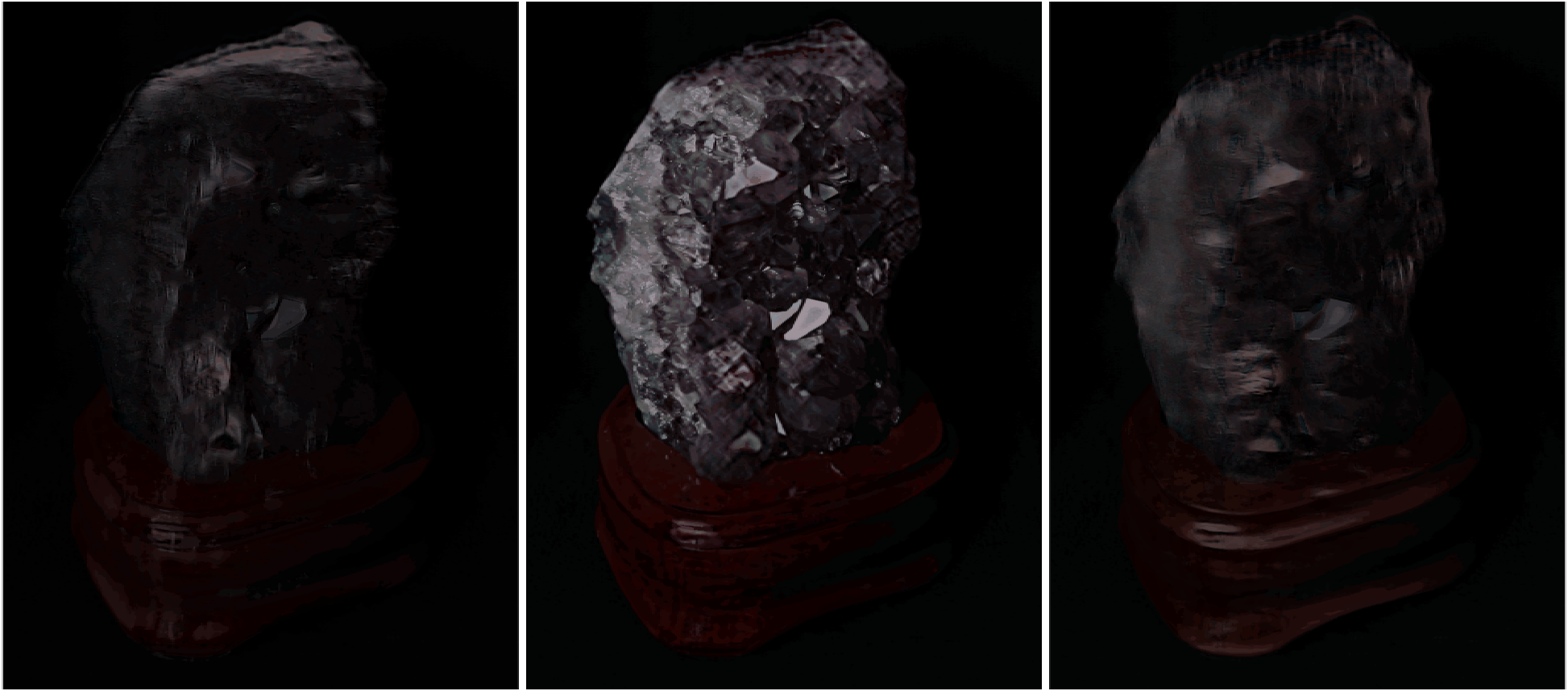
(d) $Level=3$

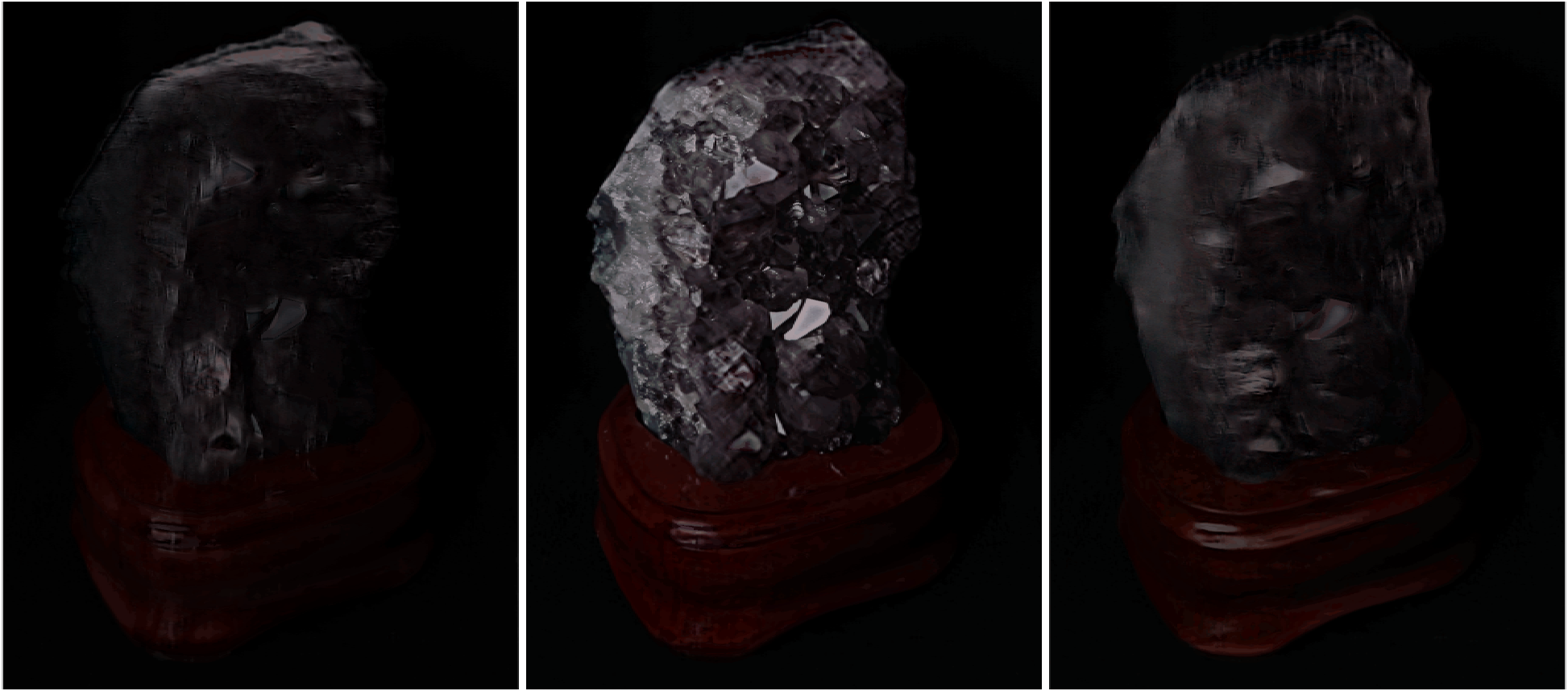
(e) $Level=4$

Figure S 5: Non-scalable and Scalable layer reconstruction of $Amethyst$.

(a) Original Layer Pattern

(b) $Level=1$

(c) $Level=2$

(d) $Level=3$

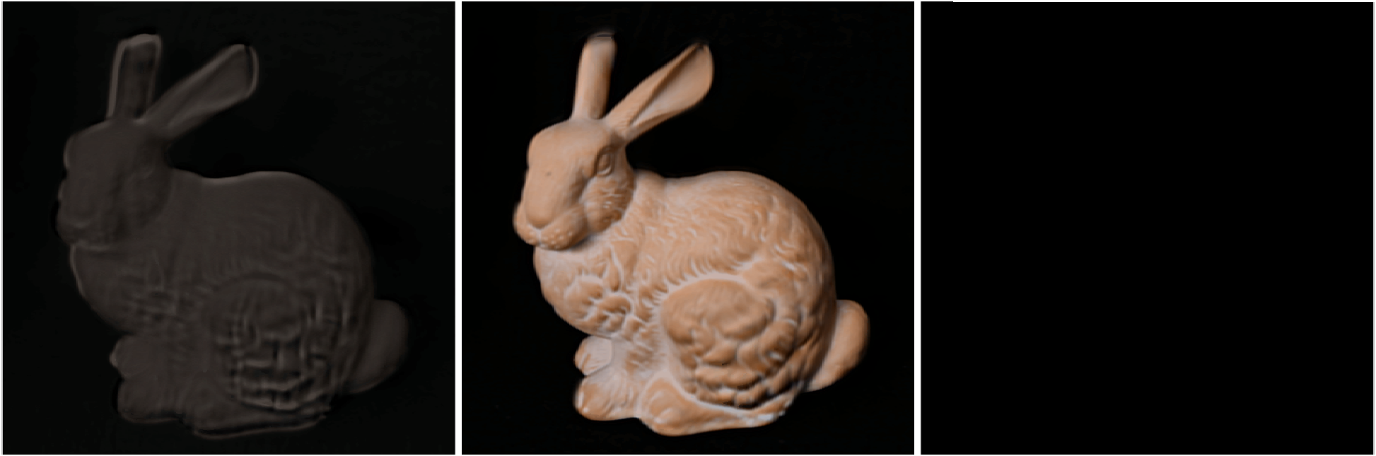
(e) $Level=4$

Figure S 6: Non-scalable and Scalable layer reconstruction of $Bunny$.

(a) Original Layer Pattern

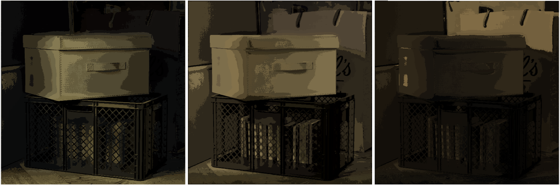
(b) $Level=1$

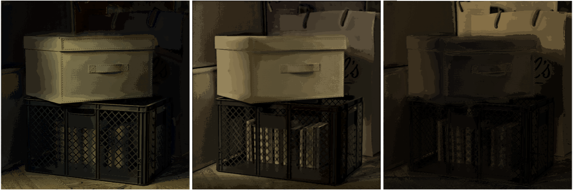
(c) $Level=2$

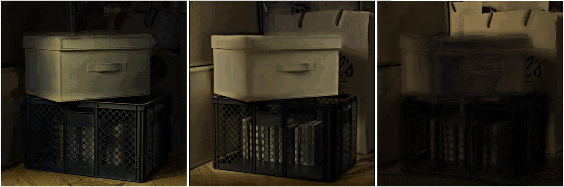
(d) $Level=3$

(e) $Level=4$

Figure S 7: Non-scalable and Scalable layer reconstruction of $Boxes$.

(a) Original Layer Pattern

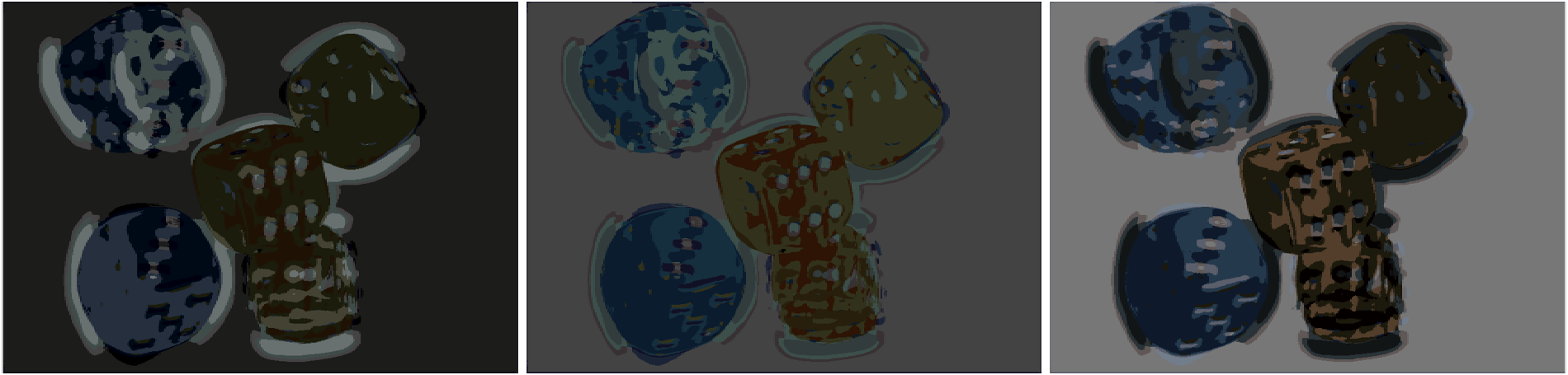
(b) $Level=1$

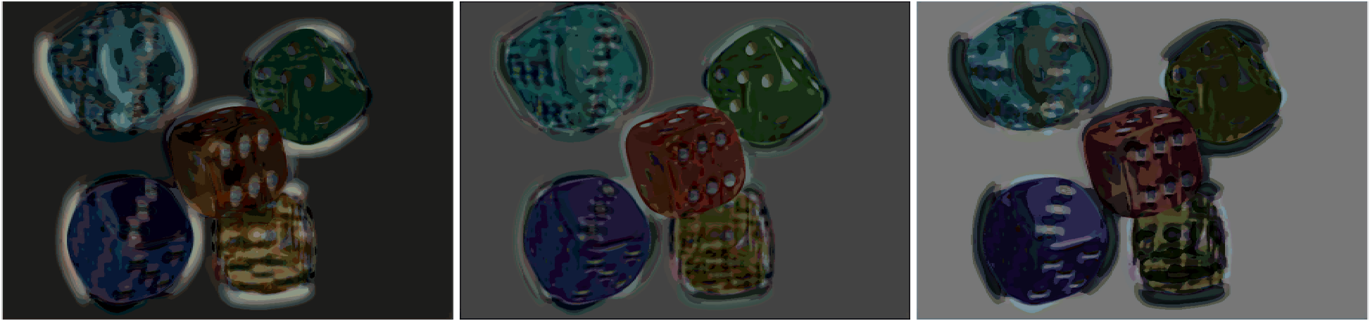
(c) $Level=2$

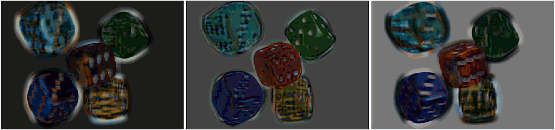
(d) $Level=3$

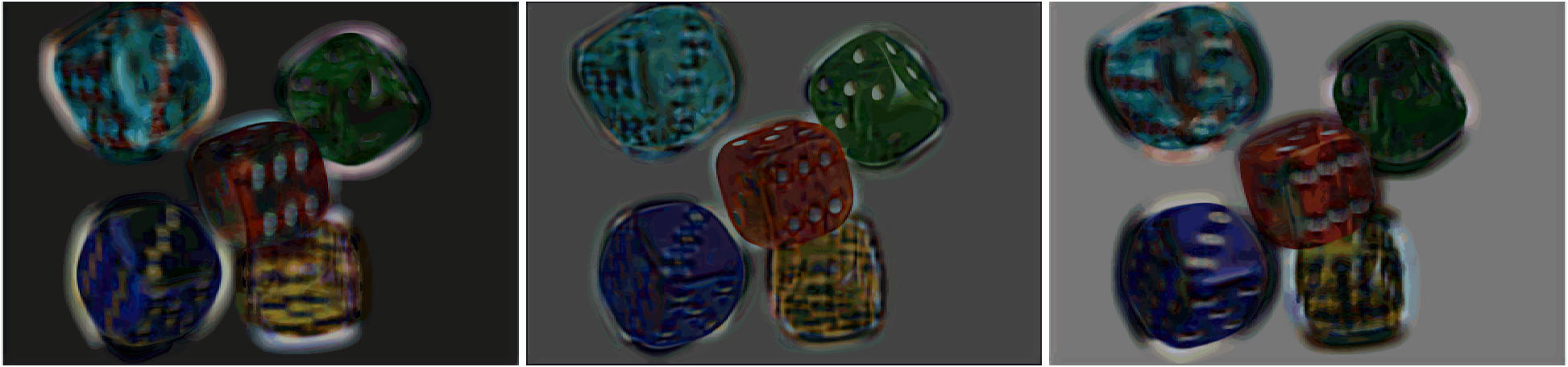
(e) $Level=4$

Figure S 8: Non-scalable and Scalable layer reconstruction of $Dice$.

(a) Original Layer Pattern

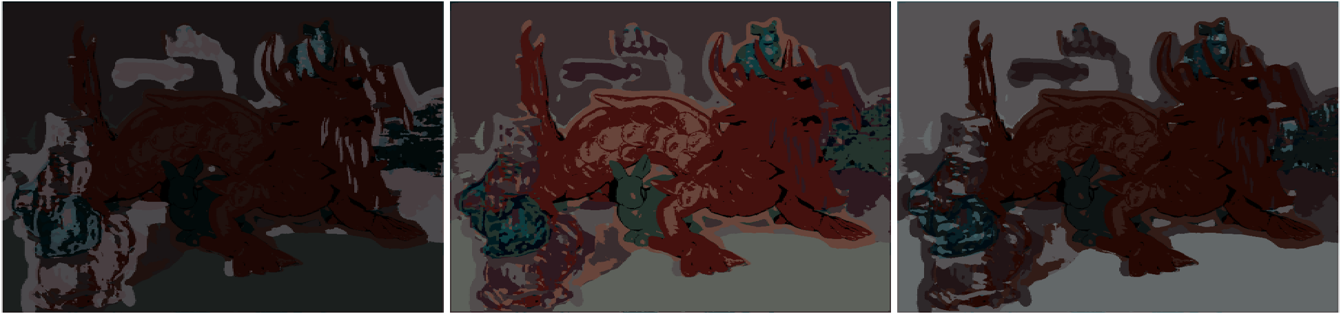
(b) $Level=1$

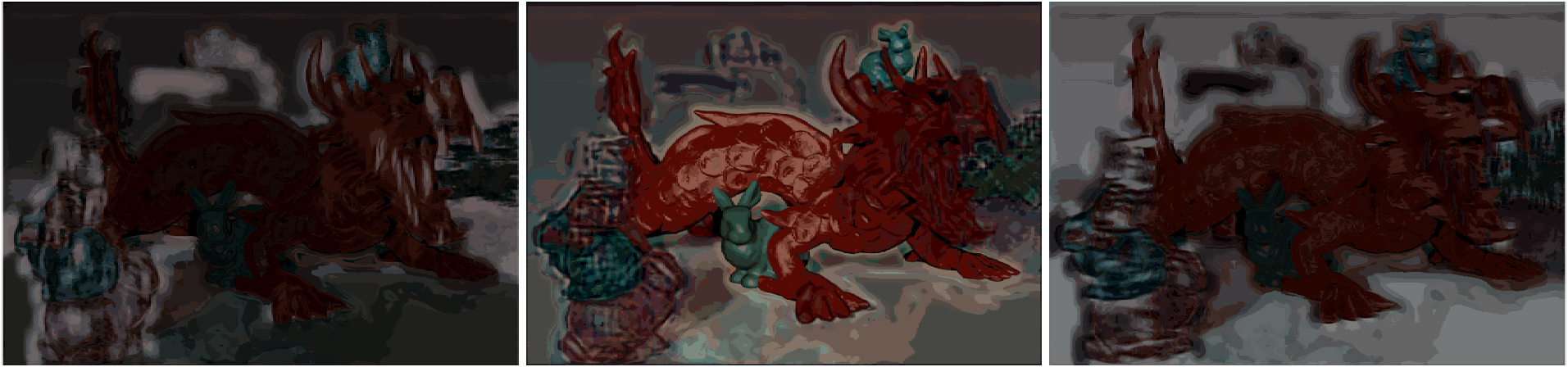
(c) $Level=2$

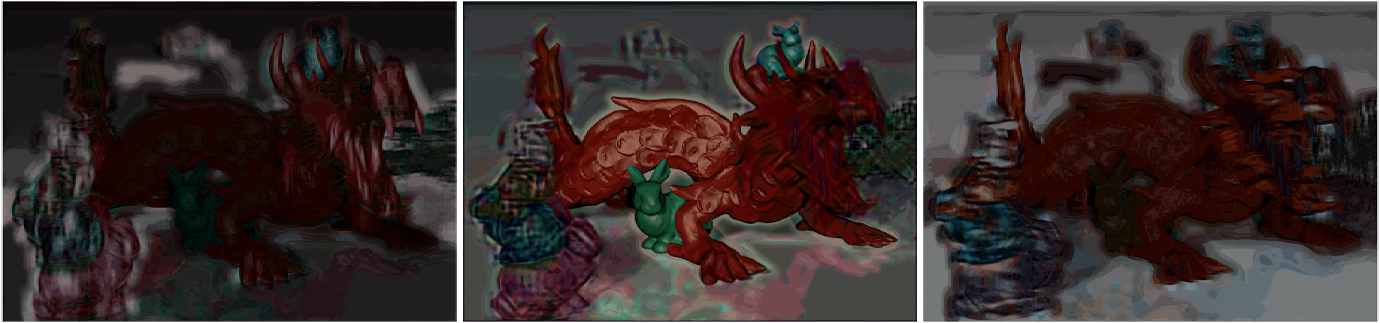
(d) $Level=3$

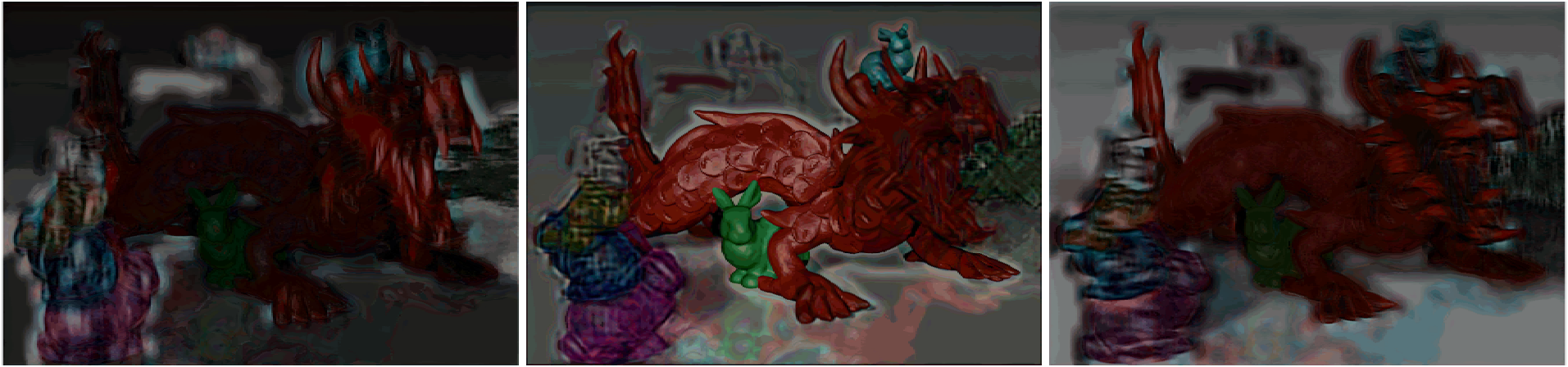
(e) $Level=4$

Figure S 9: Non-scalable and Scalable layer reconstruction of $DragonAndBunnies$.

(a) Original Layer Pattern

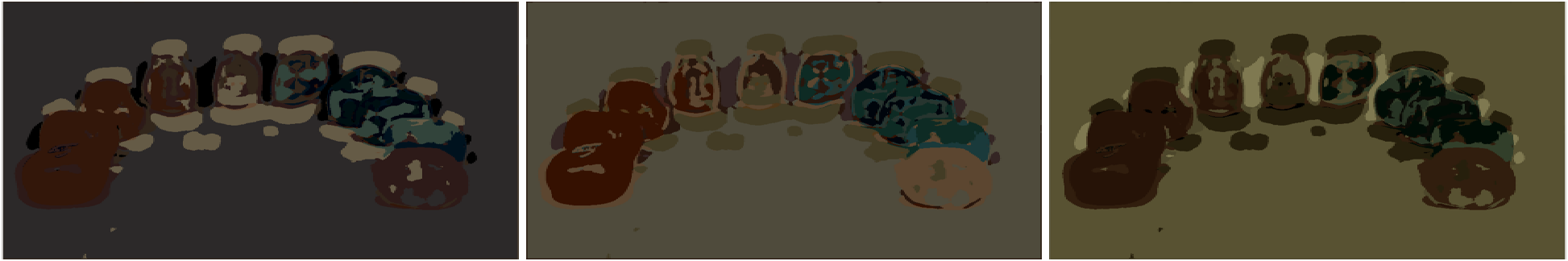
(b) $Level=1$

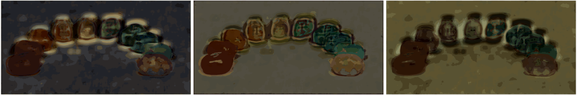
(c) $Level=2$

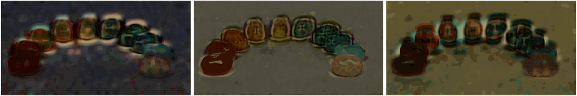
(d) $Level=3$

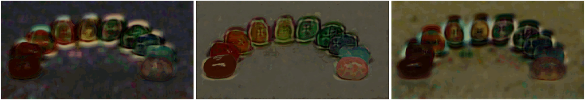
(e) $Level=4$

Figure S 10: Non-scalable and Scalable layer reconstruction of $Jellybeans$.

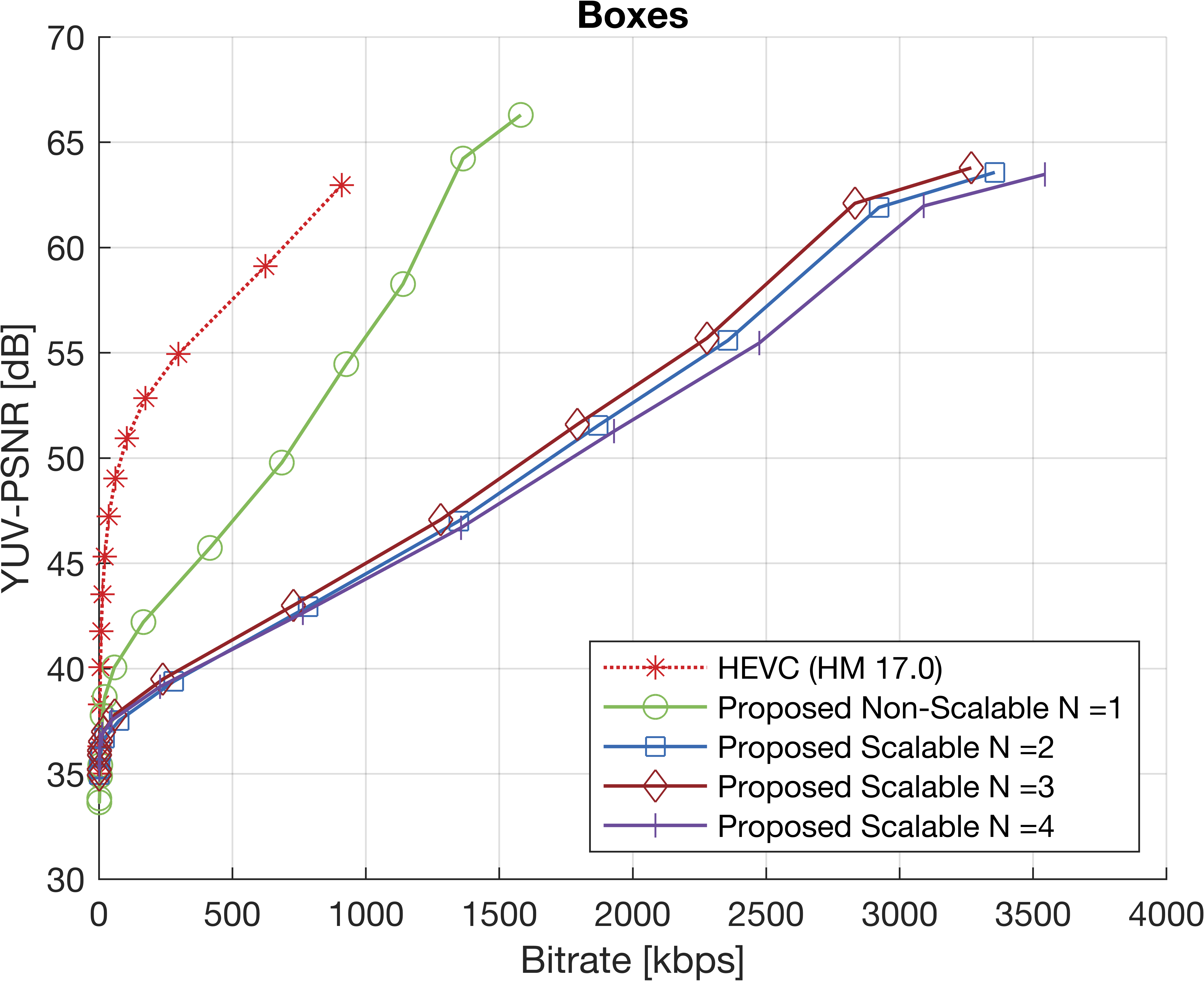
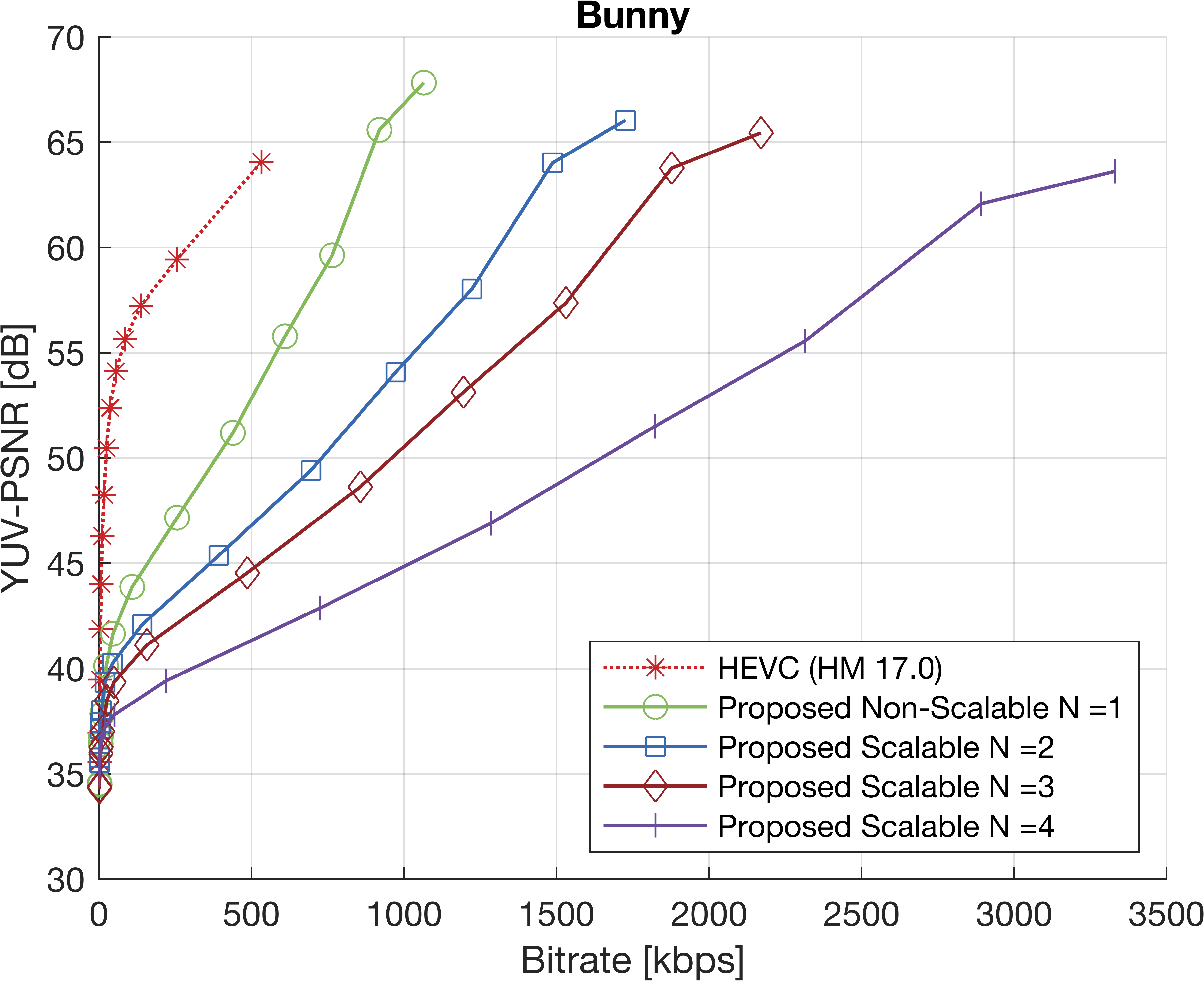
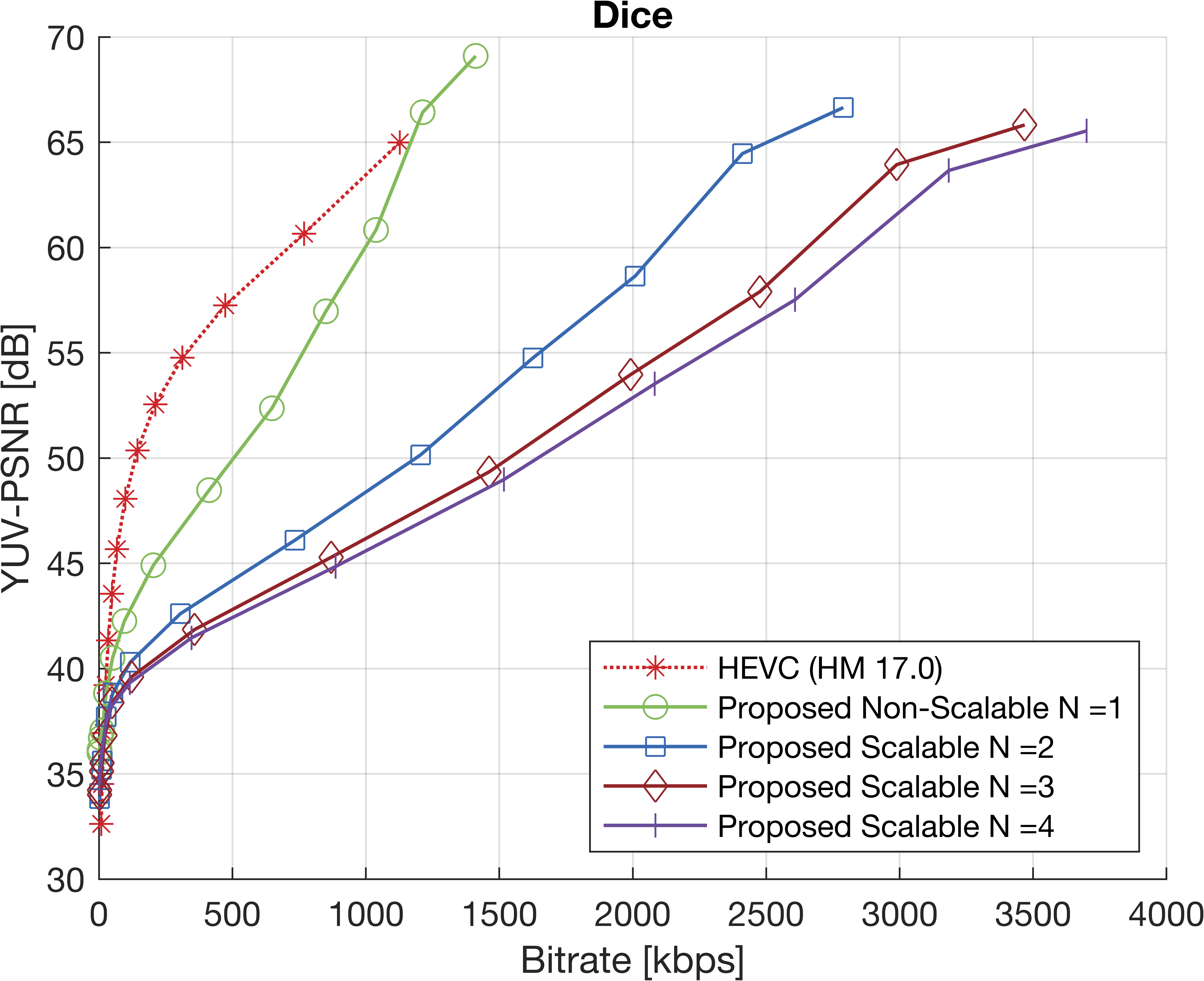
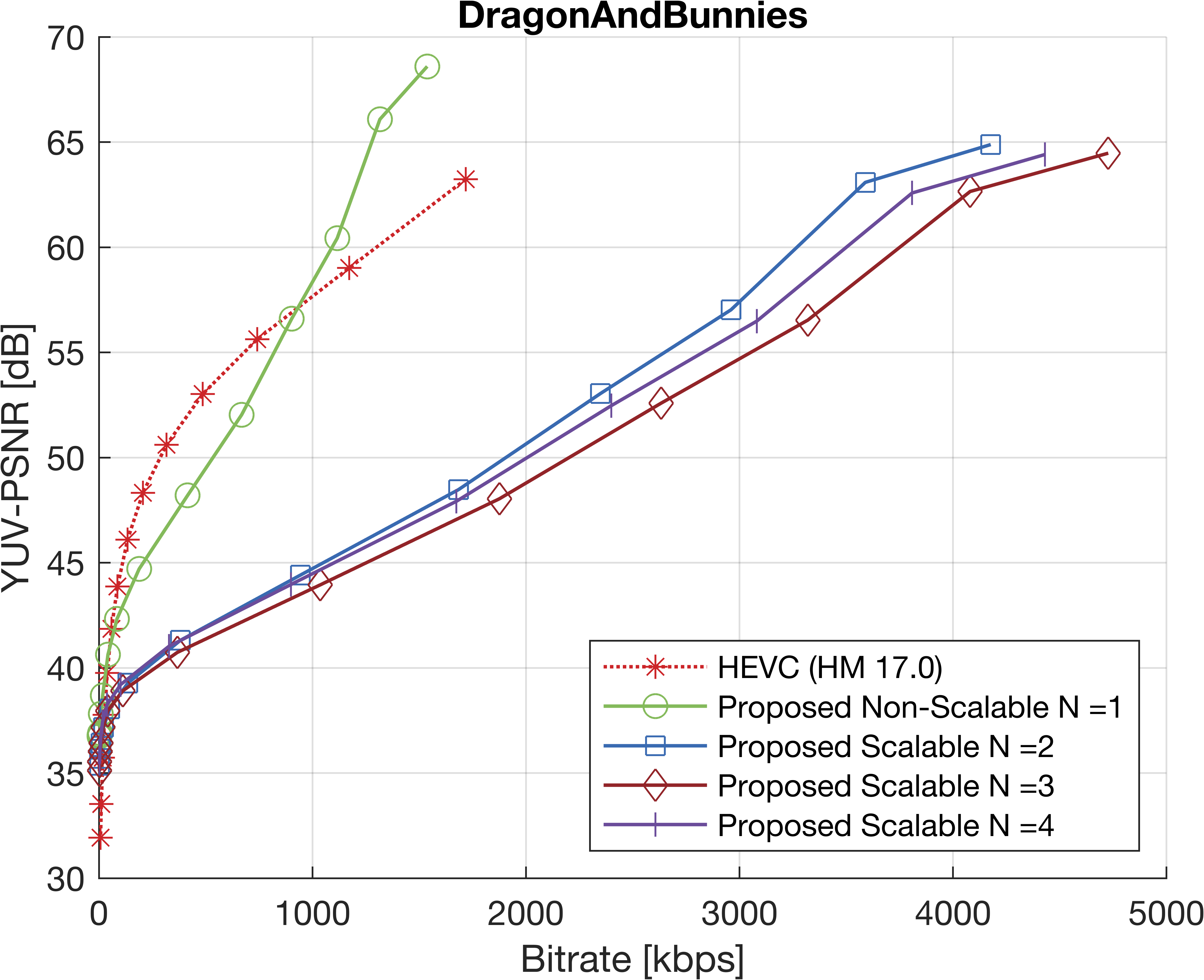
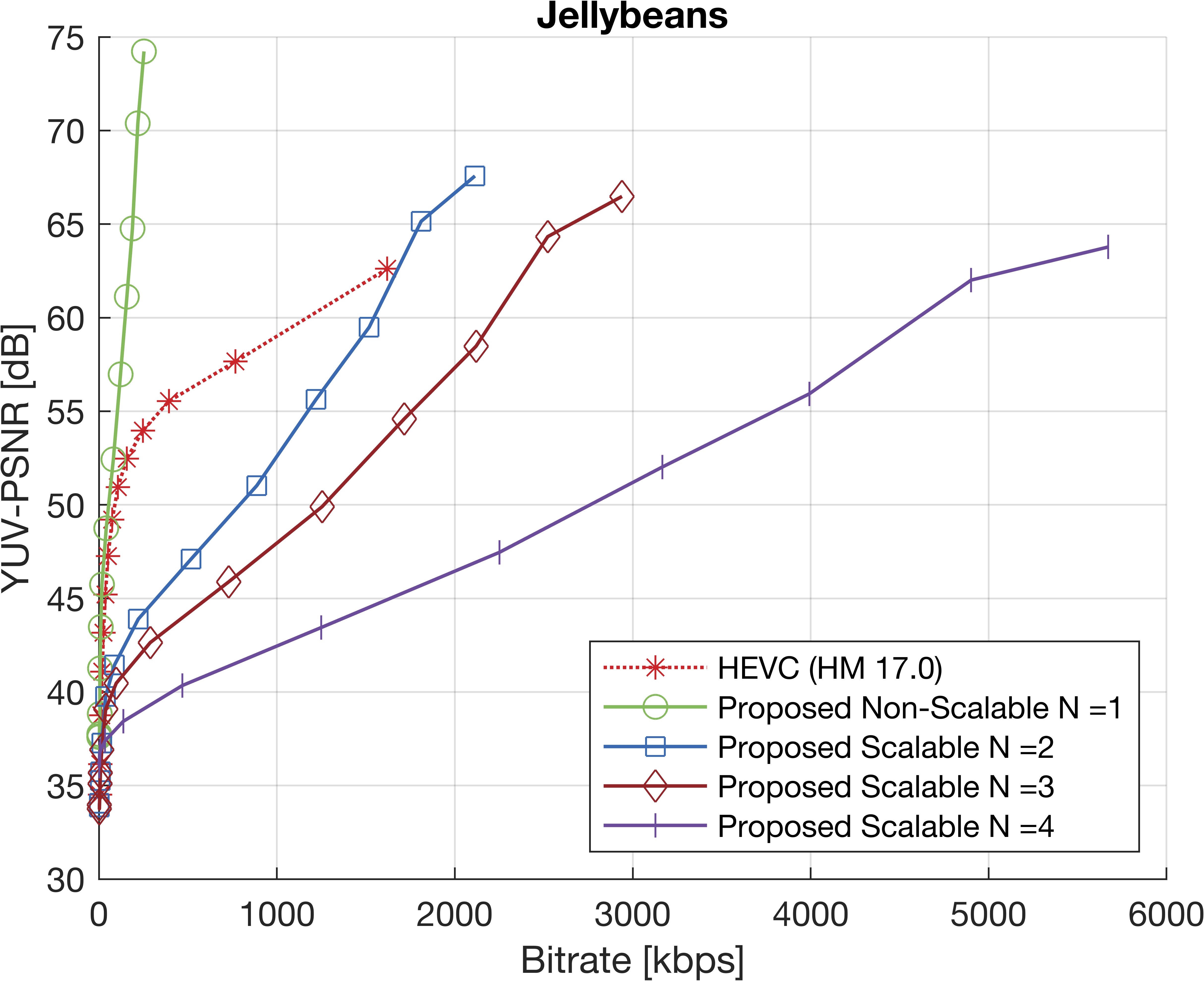
Figure S 11: The rate-distortion curve of the proposed compression scheme compared to that of standard video codec (HEVC).

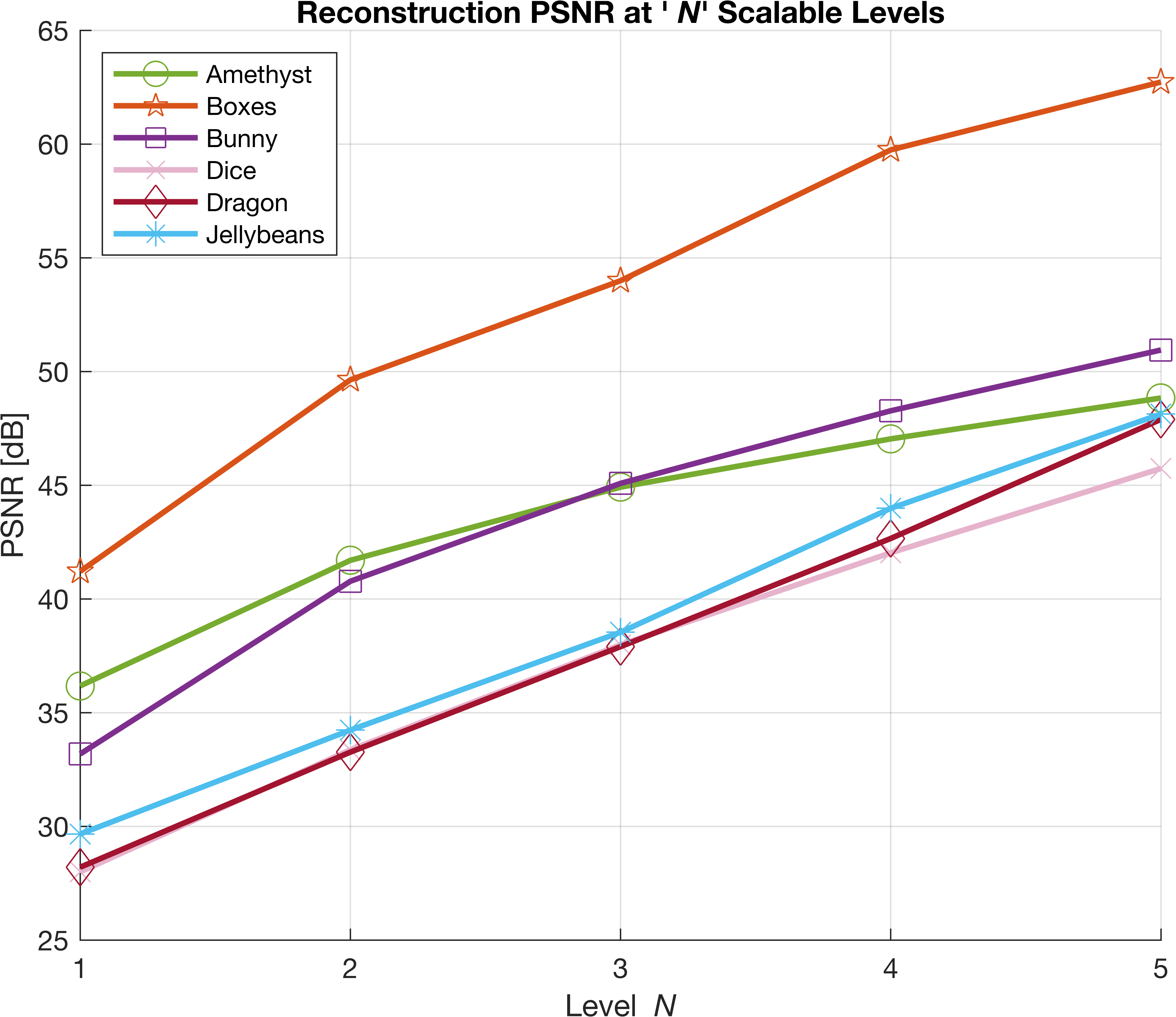
(a)

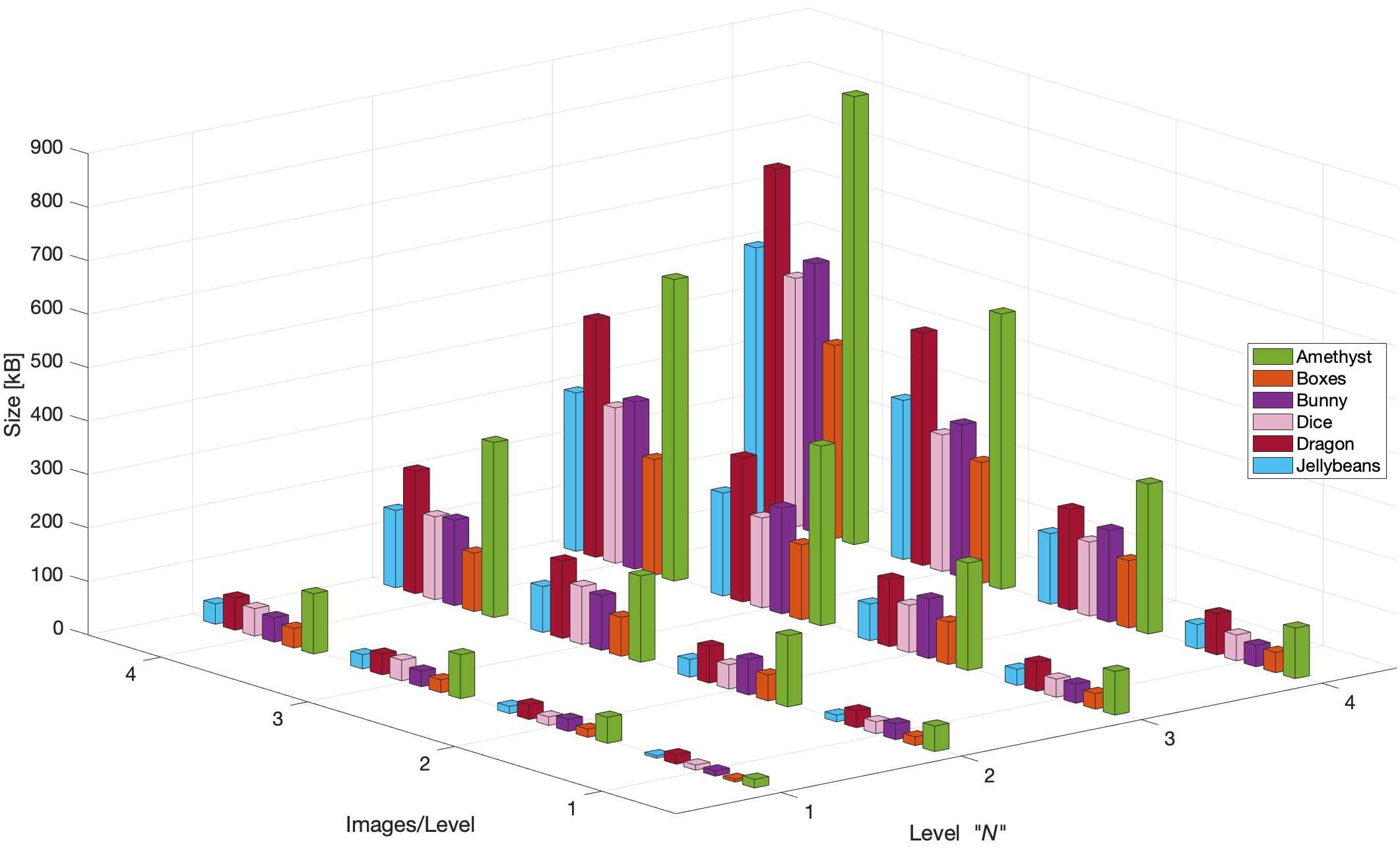
(b)

Figure S 12: Comparison of $(a)$ peak signal-to-noise ratio (PSNR) and $(b)$ sizes between scalable and non-scalable codings with $10$ binary images per level.

References

- Surman and Sun [2014] Phil Surman and Xiao Wei Sun. Towards the reality of 3d imaging and display. In 2014 3DTV-Conference, pages 1–4, 2014.
- Li et al. [2020] Tuotuo Li, Qiong Huang, Santiago Alfaro, Alexey Supikov, Joshua Ratcliff, Ginni Grover, and Ronald Azuma. Light-field displays: a view-dependent approach. In ACM SIGGRAPH 2020 Emerging Technologies, pages 1–2. 2020.
- Watanabe et al. [2019] Hayato Watanabe, Naoto Okaichi, Takuya Omura, Masanori Kano, Hisayuki Sasaki, and Masahiro Kawakita. Aktina vision: Full-parallax three-dimensional display with 100 million light rays. Scientific reports, 9(1):1–9, 2019.
- Ives [1903] Frederic E Ives. Parallax stereogram and process of making same., April 14 1903. US Patent 725,567.
- Isono et al. [1993] Haruo Isono, Minoru Yasuda, and Hideaki Sasazawa. Autostereoscopic 3-d display using lcd-generated parallax barrier. Electronics and Communications in Japan (Part II: Electronics), 76(7):77–84, 1993.
- Sakamoto and Morii [2006] Kunio Sakamoto and Tsutomu Morii. Multi-view 3d display using parallax barrier combined with polarizer. In Advanced Free-Space Optical Communication Techniques, volume 6399, pages 214–221. SPIE, 2006.
- Peterka et al. [2008] Tom Peterka, Robert L Kooima, Daniel J Sandin, Andrew Johnson, Jason Leigh, and Thomas A DeFanti. Advances in the dynallax solid-state dynamic parallax barrier autostereoscopic visualization display system. IEEE TCVG, 14(3):487–499, 2008.
- Lippmann [1908] Gabriel Lippmann. Epreuves reversibles donnant la sensation du relief. J. Phys. Theor. Appl., 7(1):821–825, 1908.
- Börner [1993] R Börner. Autostereoscopic 3d-imaging by front and rear projection and on flat panel displays. Displays, 14(1):39–46, 1993.
- McCormick [1995] M McCormick. Integral 3-d imaging for broadcast. In Proc., of the Second International Displays Workshop, pages 77–80, 1995.
- Wetzstein et al. [2012] Gordon Wetzstein, Douglas R Lanman, Matthew Waggener Hirsch, and Ramesh Raskar. Tensor displays: compressive light field synthesis using multilayer displays with directional backlighting. 2012.
- Takahashi et al. [2018] Keita Takahashi, Yuto Kobayashi, and Toshiaki Fujii. From focal stack to tensor light-field display. IEEE TIP, 27(9):4571–4584, 2018.
- Maruyama et al. [2020] Keita Maruyama, Keita Takahashi, and Toshiaki Fujii. Comparison of layer operations and optimization methods for light field display. IEEE Access, 8:38767–38775, 2020.
- Lee et al. [2016] Seungjae Lee, Changwon Jang, Seokil Moon, Jaebum Cho, and Byoungho Lee. Additive light field displays: Realization of augmented reality with holographic optical elements. 35(4), 2016. ISSN 0730-0301.
- Kramida [2015] Gregory Kramida. Resolving the vergence-accommodation conflict in head-mounted displays. IEEE TVCG, 22(7):1912–1931, 2015.
- Konrad et al. [2020] Robert Konrad, Anastasios Angelopoulos, and Gordon Wetzstein. Gaze-contingent ocular parallax rendering for virtual reality. ACM TOG, 39(2):1–12, 2020.
- Sluka et al. [2021] Tomas Sluka, Alexander Kvasov, and Tomas Kubes. Digital light-field. 2021.
- Liu et al. [2016] Dong Liu, Lizhi Wang, Li Li, Zhiwei Xiong, Feng Wu, and Wenjun Zeng. Pseudo-sequence-based light field image compression. In 2016 ICMEW, pages 1–4, 2016.
- Li et al. [2017] Li Li, Zhu Li, Bin Li, Dong Liu, and Houqiang Li. Pseudo-sequence-based 2-d hierarchical coding structure for light-field image compression. IEEE Journal of Selected Topics in Signal Processing, 11(7):1107–1119, 2017.
- Sullivan et al. [2012] Gary J Sullivan, Jens-Rainer Ohm, Woo-Jin Han, and Thomas Wiegand. Overview of the high efficiency video coding (hevc) standard. IEEE TCSVT, 22(12):1649–1668, 2012.
- Hannuksela et al. [2015] Miska M Hannuksela, Ye Yan, Xuehui Huang, and Houqiang Li. Overview of the multiview high efficiency video coding (mv-hevc) standard. In 2015 ICIP, pages 2154–2158, 2015.
- Senoh et al. [2018] Takanori Senoh, Kenji Yamamoto, Nobuji Tetsutani, and Hiroshi Yasuda. Efficient light field image coding with depth estimation and view synthesis. In EUSIPCO, pages 1840–1844, 2018.
- Huang et al. [2018] Xinpeng Huang, Ping An, Liang Shan, Ran Ma, and Liquan Shen. View synthesis for light field coding using depth estimation. In ICME, pages 1–6. IEEE, 2018.
- Hériard-Dubreuil et al. [2019] Baptiste Hériard-Dubreuil, Irene Viola, and Touradj Ebrahimi. Light field compression using translation-assisted view estimation. In Picture Coding Symposium, pages 1–5, 2019.
- Bakir et al. [2018] Nader Bakir, Wassim Hamidouche, Olivier Déforges, Khouloud Samrouth, and Mohamad Khalil. Light field image compression based on convolutional neural networks and linear approximation. In 2018 25th ICIP, pages 1128–1132, 2018.
- Wang et al. [2019] Bing Wang, Qiang Peng, Eric Wang, Kang Han, and Wei Xiang. Region-of-interest compression and view synthesis for light field video streaming. IEEE Access, 7:41183–41192, 2019.
- Jia et al. [2018] Chuanmin Jia, Xinfeng Zhang, Shanshe Wang, Shiqi Wang, and Siwei Ma. Light field image compression using generative adversarial network-based view synthesis. IEEE Journal on Emerging and Selected Topics in Circuits and Systems, 9(1):177–189, 2018.
- Liu et al. [2021] Deyang Liu, Xinpeng Huang, Wenfa Zhan, Liefu Ai, Xin Zheng, and Shulin Cheng. View synthesis-based light field image compression using a generative adversarial network. Information Sciences, 545:118–131, 2021.
- Vagharshakyan et al. [2017] Suren Vagharshakyan, Robert Bregovic, and Atanas Gotchev. Light field reconstruction using shearlet transform. IEEE transactions on pattern analysis and machine intelligence, 40(1):133–147, 2017.
- Ahmad et al. [2020] Waqas Ahmad, Suren Vagharshakyan, Mårten Sjöström, Atanas Gotchev, Robert Bregovic, and Roger Olsson. Shearlet transform-based light field compression under low bitrates. IEEE TIP, 29:4269–4280, 2020.
- Chen et al. [2020] Yilei Chen, Ping An, Xinpeng Huang, Chao Yang, Deyang Liu, and Qiang Wu. Light field compression using global multiplane representation and two-step prediction. IEEE Signal Processing Letters, 27:1135–1139, 2020.
- Teh and Hinton [2000] Yee Whye Teh and Geoffrey E Hinton. Rate-coded restricted boltzmann machines for face recognition. Advances in neural information processing systems, 13, 2000.
- Hinton and Salakhutdinov [2006] Geoffrey E Hinton and Ruslan R Salakhutdinov. Reducing the dimensionality of data with neural networks. science, 313(5786):504–507, 2006.
- Komatsu et al. [2018] Koji Komatsu, Keita Takahashi, and Toshiaki Fujii. Scalable light field coding using weighted binary images. In IEEE ICIP, pages 903–907, 2018.
- Toth [2000] Paolo Toth. Optimization engineering techniques for the exact solution of np-hard combinatorial optimization problems. European journal of operational research, 125(2):222–238, 2000.
- Shang et al. [2014] Chao Shang, Fan Yang, Dexian Huang, and Wenxiang Lyu. Data-driven soft sensor development based on deep learning technique. Journal of Process Control, 24(3):223–233, 2014.
- Hinton [2002] Geoffrey E Hinton. Training products of experts by minimizing contrastive divergence. Neural computation, 14(8):1771–1800, 2002.
- Vaish and Adams [2008] Vaibhav Vaish and Andrew Adams. The (new) stanford light field archive. Computer Graphics Laboratory, Stanford University, 6(7):3, 2008.
- Honauer et al. [2017] Katrin Honauer, Ole Johannsen, Daniel Kondermann, and Bastian Goldluecke. A dataset and evaluation methodology for depth estimation on 4d light fields. In Computer Vision–ACCV, pages 19–34, 2017.
- Marwah et al. [2013] Kshitij Marwah, Gordon Wetzstein, Yosuke Bando, and Ramesh Raskar. Compressive light field photography using overcomplete dictionaries and optimized projections. ACM TOG, 32(4):1–12, 2013.
- Bjontegaard [2001] Gisle Bjontegaard. Calculation of average psnr differences between rd-curves. VCEG-M33, 2001.