Quantum steering in a star network

Abstract

In this work, we will consider the star network scenario where the central party is trusted while all the edge parties (with a number of $n$) are untrusted. Network steering is defined with an $n$ local hidden state model which can be viewed as a special kind of $n$ local hidden variable model. Three different types of sufficient criteria, nonlinear steering inequality, linear steering inequality, and Bell inequality, will be constructed to verify the quantum steering in a star network. Based on the linear steering inequality, it is found that the network steering can be demonstrated even though the trusted party performs a fixed measurement.

I Introduction

In 1930s, the concept of steering was introduced by Schrödinger [1] as a generalization of the Einstein-Podolsky-Rosen (EPR) paradox [2]. For a bipartite state, steering infers that an observer on one side can affect the state of the other spatially separated system by local measurements. In 2007, a standard formalism of quantum steering was developed by Wiseman, Jones and Doherty [3]. In quantum information processing, EPR steering can be defined as the task for a referee to determine whether one party shares entanglement with a second untrusted party [3, 4, 5]. Quantum steering is a type of quantum nonlocality that is logically distinct from inseparability [6, 7] and Bell nonlocality [8].

In the last decade, the investigation of nonlocality has moved beyond Bell’s theorem to consider more sophisticated experiments that involve several independent sources which distribute shares of physical systems among many parties in a network [9, 10, 11]. The discussions, which are about the main concepts, methods, results and future challenges in the emerging topic of Bell in networks, can be found in the review article [12]. The independence of various sources leads to nonconvexity in the space of relevant correlations [13, 14, 15, 16, 17, 18, 19, 20, 21].

The simplest network scenario is provided by entanglement swapping [22]. To contrast classical and quantum correlation in this scenario, the so-called bilocality assumption where the classical models consist of two independent local hidden variables (LHV), has been considered [9, 10]. The generalization of the bilocality scenario to network, is the so-called $n$-locality scenario, where the number of independent sources of states is increased to arbitrary $n$ [14, 15, 16, 23, 24, 25]. Some new interesting effects, such as the possibility to certify quantum nonlocality “without inputs”, are offered by the network structure [10, 11, 26, 27].

The quantum network scenarios, where some of the parties are trusted while the others are untrusted, are naturally connected to the notion of quantum steering. Though the notion of multipartite steering has been previously considered [28, 29], the steering in the scenario of network with independent sources is seldom discussed. In the recent work [30], focusing on the linear network with trusted end points and intermediated untrusted parties who perform a fixed measurement, the authors introduced the network steering and network local hidden state models. Motivated by the work in Ref. [30], the steering in a star network will be considered here.

An important example for a multiparty network is a star-shaped configuration. Such a star network is composed of a central party that is separately connected, via a number of $n$ independent bipartite sources, to $n$ edge parties. Correlations in the network arise through the central party jointly measuring the $n$ independent shares received from the sources and edge parties locally measuring the single shares received from the corresponding sources. In the present work, we consider the star network scenario where the central party is trusted while all the edge parties are untrusted.

In this work, the quantum steering in a star network is defined by introducing of an $n$-LHS model. It will be shown that this $n$-LHS model can be viewed as a special kind of $n$-LHV model developed in [14, 15, 16, 23, 24, 25]. Besides the $n$-LHS model, we will focus on how to verify the quantum steering in the star network. Three different types of sufficient criteria, linear steering inequality, nonlinear steering inequality, and Bell inequality, will be designed. Unlike detecting steering with single source, it will be shown that the network steering can be demonstrated even for the case taht a fixed measurement is performed by the trusted central party.

The content of this work is organized as follows. In Sec. II, we give a brief review on the definition of steering in bipartite system. In Sec. III, for a star network scenario where the central party is trusted while all the edge parties are untrusted, network steering is defined with an $n$-LHS model. To verify the network steering, three different types of sufficient criteria, the nonlinear steering inequality, linear steering inequality, and Bell inequality, are designed in Sec. IV, Sec. V, and Sec. VI, respectively. Finally, we end our work with a short conclusion.

II Preliminary

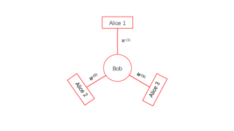
For convenience, in a star network shown in Fig. 1, we call the observer in the central party as Bob while the observers in the edge parties as Alices. Using $W^{(\mu)}$ ($\mu=1,2...,n$) to denote the source state shared by the $\mu$th Alice and Bob, the state in the star network can be expressed as

$$W=\bigotimes_{\mu=1}^{n}W^{(\mu)}.$$ (1)

Figure 1: A star network is composed of a central party and $n$ edge parties, and via a number of $n$ independent bipartite sources, the central party is separately connected to the $n$ edge parties. The figure above is depicted for a star-shaped network with $n=3$, where each edge observer shares a bipartite state $W^{(\mu)}$ $(\mu=1,2,3)$ with the central observer.

Before defining quantum steering in the star network, some necessary conventions are required. First, for the bipartite state $W^{(\mu)}$, the $\mu$th Alice can perform $N$ measurements on her side, labelled by $x_{\mu}=1,2,...,N$, each having $m$ outcomes $a_{\mu}=0,1,...,m-1$, and the measurements are represented by $\hat{\Pi}^{(\mu)}_{a_{\mu}|x_{\mu}}$, $\sum_{a_{\mu}=0}^{m-1}\hat{\Pi}^{(\mu)}_{a_{\mu}|x_{\mu}}=I_{d}$, with $I_{d}$ the identity operator for the local $d$-dimensional Hilbert space. For a bipartite state $W^{(\mu)}$, the unnormalized postmeasurement states prepared for Bob are given by

$$\tilde{\rho}^{(\mu)}_{a_{\mu}|x_{\mu}}={\rm{Tr}}_{\mathrm{A}}\left[\left(\hat{\Pi}^{(\mu)}_{a_{\mu}|x_{\mu}}\otimes I_{d}\right)W^{(\mu)}\right].$$ (2)

The set of the unnormalized states, $\left\{\tilde{\rho}^{(\mu)}_{a_{\mu}|x_{\mu}}\right\}$, is usually called an assemblage.

In 2007, Wiseman, Jones and Doherty formally defined quantum steering as the possibility of remotely generating ensembles that could not be produced by a local hidden state (LHS) model [3]. An LHS model refers to the case where a source sends a classical message $\xi_{\mu}$ to the $\mu$th Alice, and a corresponding quantum state $\rho^{(\mu)}_{\xi_{\mu}}$ to Bob. Given that the $\mu$th Alice decides to performs the measurement $x_{\mu}$, the variable $\xi_{\mu}$ instructs the output $a_{\mu}$ of Alice’s apparatus with the probability $\mathfrak{p}^{(\mu)}\left(a_{\mu}|x_{\mu},\xi_{\mu}\right)$. The variable $\xi_{\mu}$ can also be interpreted as a local hidden variable (LHV) and chosen according to a probability distribution $\Omega^{(\mu)}(\xi_{\mu})$. Bob does not have access to the classical variable $\xi_{\mu}$, and his final assemblage is composed by

$$\tilde{\rho}^{(\mu)}_{a_{\mu}|x_{\mu}}=\int d\xi_{\mu}\Omega^{(\mu)}(\xi_{\mu})\mathfrak{p}^{(\mu)}(a_{\mu}|x_{\mu},\xi_{\mu})\rho^{(\mu)}_{\xi_{\mu}},$$ (3)

with the constraints

$$\sum_{a_{\mu}}\mathfrak{p}^{(\mu)}(a_{\mu}|x_{\mu},\xi_{\mu})=1,\ \ \int d\xi_{\mu}\Omega^{(\mu)}(\xi_{\mu})=1.$$ (4)

In this paper, the definition of steering from the $\mu$th Alice to Bob is directly cited from the review article [31]: An assemblage is said to demonstrate steering if it does not admit a decomposition of the form in Eq. (3). Furthermore, a quantum state $W^{(\mu)}$ is said to be steerable from $\mu$th Alice to Bob if the experiments in $\mu$th Alice’s part produce an assemblage that demonstrate steering. On the contrary, an assemblage is said to be LHS if it can be written as in Eq. (3), and a quantum state is said to be unsteerable if an LHS assemblage is generated for all local measurements.

Joint measurability, which is a natural extension of commutativity for general measurement, was studied extensively for a few decades before steering was formulated in its modern form [32]. Its relation with quantum steering has been discussed in recent works [33, 34, 35, 36]. A set of measurements $\left\{\hat{M}^{(\mu)}_{a_{\mu}|x_{\mu}}\right\}$, where $\sum_{a_{\mu}}\hat{M}^{(\mu)}_{a_{\mu}|x_{\mu}}=I$ holds for each setting $x_{\mu}$, is jointly measurable if there exists a set of POVMs $\left\{\hat{M}^{(\mu)}_{\lambda}\right\}$, such that $\hat{M}^{(\mu)}_{a_{\mu}|x_{\mu}}=\sum_{\lambda}\pi(\lambda)p\left(a_{\mu}|x_{\mu},\lambda\right)\hat{M}_{\lambda}$ for all $a_{\mu}$ and $x_{\mu}$, with $\pi(\lambda)$ and $p\left(a_{\mu}|x_{\mu},\lambda\right)$ the probability distributions. Otherwise, $\left\{\hat{M}^{(\mu)}_{a_{\mu}|x_{\mu}}\right\}$ is said to be incompatible.

For the bipartite state $W^{(\mu)}$ shared by Bob and the $\mu$th Alice, one can denote $\rho_{\mathrm{B}}$ to be the reduced density matrix on Bob’s side and the purification of $\rho_{\mathrm{B}}^{*}$ is denoted by $|\Psi^{(\mu)}\rangle$, where $\rho_{\mathrm{B}}^{*}$ is the complex conjugate of $\rho_{\mathrm{B}}$. The state $W^{(\mu)}$ can be expressed as

$$W^{(\mu)}=\varepsilon\otimes\mathcal{I}\left(|\Psi^{(\mu)}\rangle\langle\Psi^{(\mu)}|\right),$$ (5)

by introducing a quantum channel $\varepsilon$, $\varepsilon(\rho)=\sum_{m}\hat{E}_{m}\rho\hat{E}^{\dagger}_{m}$ with the Kraus operators $\left\{\hat{E}_{m}\right\}$, and $\mathcal{I}$ is an identity map. With the definition that $\hat{M}^{(\mu)}_{a_{\mu}|x_{\mu}}=\sum_{m}\hat{E}_{m}^{\dagger}\hat{\Pi}^{(\mu)}_{a_{\mu}|x_{\mu}}\hat{E}_{m}$, it has been shown that the conditional states in Eq. (2) can be reexpressed as

$$\tilde{\rho}^{(\mu)}_{a_{\mu}|x_{\mu}}=\rho^{*}_{\mathrm{B}}\hat{M}^{(\mu)}_{a_{\mu}|x_{\mu}}\left(\rho^{*}_{\mathrm{B}}\right)^{\dagger}.$$ (6)

If $\left\{\tilde{\rho}^{(\mu)}_{a_{\mu}|x_{\mu}}\right\}$ admits an LHS model, by an explicit definition of the inverse matrix of $\rho_{\mathrm{B}}$, one may find that the measurement $\left\{\hat{M}^{(\mu)}_{a_{\mu}|x_{\mu}}\right\}$ is jointly measurable [32, 34].

For the state $W^{(\mu)}$, the measurement performed by the $\mu$th Alice is denoted by $\hat{\Pi}^{(\mu)}_{a_{\mu}|x_{\mu}}$, and if each $a_{\mu}$ takes the value 0 or 1, one can introduce an operator

$$\hat{A}^{(\mu)}_{x_{\mu}}=\hat{\Pi}^{(\mu)}_{0|x_{\mu}}-\hat{\Pi}^{(\mu)}_{1|x_{\mu}}.$$ (7)

Similarly, the measurement performed by Bob is denoted by $\hat{\Pi}^{(\mu)}_{b_{\mu}|y_{\mu}}$, and if $b_{\mu}$ takes the value 0 or 1, another operator $\hat{B}_{y_{\mu}}$ can also be introduced

$$\hat{B}^{(\mu)}_{y_{\mu}}=\hat{\Pi}^{(\mu)}_{0|y_{\mu}}-\hat{\Pi}^{(\mu)}_{1|y_{\mu}}.$$ (8)

For the case $n=2$, let $\hat{O}=\left(\hat{A}^{(1)}_{x_{1}}\otimes\hat{B}^{(1)}_{y_{1}}\right)\otimes\left(\hat{A}^{(2)}_{x_{2}}\otimes\hat{B}^{(2)}_{y_{2}}\right)$ to be an observable for the state $W=\otimes_{\mu=1}^{2}W^{(\mu)}$. Formally, one can introduce a unitary transformation $U$, which is defined by $\hat{O}^{\prime}\equiv U\hat{O}U^{\dagger}=\left(\hat{A}^{(1)}_{x_{1}}\otimes\hat{A}^{(2)}_{x_{2}}\right)\otimes\left(\hat{B}^{(1)}_{y_{1}}\otimes\hat{B}^{(2)}_{y_{2}}\right)$ and $W^{\prime}=U^{\dagger}WU$, to express the expectation ${\rm{Tr}}\left(\hat{O}W\right)$ as $\langle\hat{O}^{\prime}\rangle\equiv{\rm{Tr}}\left(\hat{O}^{\prime}W^{\prime}\right)$. Certainly, the above definition can be easily generalized for arbitrary $n$.

III $n\rightarrow 1$ steering in a star network

In this work, the quantum steering in the star network is defined as: The state $W$ in Eq. (1) is said to be $n\rightarrow 1$ steerable iff among the set of all source states $\{W^{(\mu)}\}_{\mu=1}^{n}$, there exists at least one source state $W^{(\mu)}$ which is one-way steerable from the $\mu$th Alice to Bob. Otherwise, for all the possible local measurements $\left\{\otimes_{\mu=1}^{n}\hat{\Pi}^{(\mu)}_{a_{\mu}|x_{\mu}}\right\}$ performed by the edge observers, the assemblage of conditional states $\left\{\otimes^{n}_{\mu=1}\tilde{\rho}^{(\mu)}_{a_{\mu}|x_{\mu}}\right\}$ should admit an $n$-LHS model,

$$\bigotimes^{n}_{\mu=1}\tilde{\rho}^{(\mu)}_{a_{\mu}|x_{\mu}}=\bigotimes^{n}_{\mu=1}\int d\xi_{\mu}\Omega^{(\mu)}(\xi_{\mu})\mathfrak{p}^{(\mu)}(a_{\mu}|x_{\mu},\xi_{\mu}))\rho^{(\mu)}_{\xi_{\mu}}.$$ (9)

Formally, the POVMs performed by Bob can be denoted by $\hat{\Pi}^{b}_{y}$ , $\sum_{b}\hat{\Pi}^{b}_{y}=I$, and the denotations $\bar{a}=a_{1}a_{2}...a_{n}$, $\bar{x}=x_{1}x_{1}...x_{n}$, and $\bar{\xi}=\xi_{1}\xi_{2}...\xi_{n}$ can be introduced. Within the $n$-LHS model, the expectation $p(\bar{a},b|\bar{x},y)$ of the operator $\left(\otimes_{\mu=1}^{n}\hat{\Pi}^{(\mu)}_{a_{\mu}|x_{\mu}}\right)\otimes\hat{\Pi}^{b}_{y}$ can be expressed as

$$p(\bar{a},b|\bar{x},y)=\int d\bar{\xi}\left[\prod_{\mu=1}^{n}\Omega^{(\mu)}(\xi_{\mu})\mathfrak{p}^{(\mu)}(a_{\mu}|x_{\mu},\xi_{\mu})\right]\mathfrak{p}(b|y,\bar{\xi}),$$

$$\mathfrak{p}(b|y,\bar{\xi})={\rm{Tr}}\left[\hat{\Pi}^{b}_{y}\left(\bigotimes^{n}_{\mu=1}\tilde{\rho}^{(\mu)}_{\xi_{\mu}}\right)\right],$$ (10)

where $d\bar{\xi}=d\xi_{1}d\xi_{2}...d\xi_{\mu}...d\xi_{n}$. In practice, if the set of probabilities $\left\{p(\bar{a}|\bar{x},b|y)\right\}$ does not admit the model above, one can conclude that the state $W$ is $n\rightarrow 1$ steerable.

One of the main reasons for us to introduce the $n\rightarrow 1$ steering is that it represents a weak form of the $n$-nonlocality. Let $\lambda_{\mu}$ be LHV for the $\mu$th resource $W^{(\mu)}$, $\int d\lambda_{\mu}\omega^{(\mu)}(\lambda_{\mu})=1$, and $\bar{\lambda}=\lambda_{1}\lambda_{2}...\lambda_{n}$. If

$$p(\bar{a},b|\bar{x},y)=\int d\bar{\lambda}\left[\prod_{\mu=1}^{n}\omega^{(\mu)}(\lambda_{\mu}){p}^{(\mu)}(a_{\mu}|x_{\mu},\lambda_{\mu})\right]{p}(b|y,\bar{\lambda}),$$ (11)

with $d\bar{\lambda}=d\lambda_{1}d\lambda_{2}...d\lambda_{\mu}...d\lambda_{n}$, where ${p}^{(\mu)}(a_{\mu}|x_{\mu},\lambda_{\mu})$ and ${p}(b|y,\bar{\lambda})$ are the predetermined values of the operators $\hat{\Pi}^{(\mu)}_{a_{\mu}|x_{\mu}}$ and $\hat{\Pi}^{b}_{y}$ within the $n$-LHV model, respectively, the probabilities $p(\bar{a},b|\bar{x},y)$ admit the $n$-LHV model [14, 15, 16, 23, 24, 25]. Otherwise, if the set of correlations $\left\{p(\bar{a},b|\bar{x},y)\right\}$ do not admit the $n$-LHV model, it is said to be $n$-nonlocal. Obviously, the $n$-LHS model can be viewed as a special kind of $n$-LHV model, where for the trusted parties, the quantum mechanics is allowed, say, $\mathfrak{p}(b|y,\bar{\xi})={\rm{Tr}}\left[\hat{\Pi}^{b}_{y}\left(\otimes^{n}_{\mu=1}{\rho}^{(\mu)}_{\xi_{\mu}}\right)\right]$. In other words, if the state $W$ is $n$-nonlocal, it must be $n\rightarrow 1$ steerable.

In the following, we will focus on the case where each independent source state is a two-qubit state and develop several types of sufficient criteria to verify the $n\rightarrow 1$ steering.

IV non-linear steering inequality

For $n=1$, there is a well-known non-linear steering inequality [37]

$$\sqrt{\left\langle\left(\hat{A}_{1}+\hat{A}_{2}\right)\bigotimes\hat{B}_{1}\right\rangle^{2}+\left\langle\left(\hat{A}_{1}+\hat{A}_{2}\right)\bigotimes\hat{B}_{2}\right\rangle^{2}}$$

$$+\sqrt{\left\langle\left(\hat{A}_{1}-\hat{A}_{2}\right)\bigotimes\hat{B}_{1}\right\rangle^{2}+\left\langle\left(\hat{A}_{1}-\hat{A}_{2}\right)\bigotimes\hat{B}_{2}\right\rangle^{2}}\leq 2,$$

where mutually unbiased measurements are performed on Bob’s site [37]. This inequality has a peculiar property: If it is violated, the state also violates the original CHSH inequality [38]. Next, an inequality can be constructed to verify the $n\rightarrow 1$ steering, and this inequality can be viewed as a generalization of the one in Eq. (IV) above.

Let $\sigma^{(\mu)}_{j}$, with $j=1,2,3$, be the Pauli matrices for the $\mu$th source state $W^{(\mu)}$. $\bm{r}^{(\mu)}_{x_{\mu}}$ is a three-dimensional vector in $\mathbb{R}^{3}$, $\bm{r}^{(\mu)}_{x_{\mu}}=\left(r^{(\mu)}_{x_{\mu}1},r^{(\mu)}_{x_{\mu}2},r^{(\mu)}_{x_{\mu}3}\right)^{\mathrm{T}}$, and the Euclidean norm of $\bm{r}^{(\mu)}_{x_{\mu}}$ is denoted by $\left|\left|\bm{r}^{(\mu)}_{x_{\mu}}\right|\right|\equiv\sqrt{\sum_{j=1}^{3}\left(r^{(\mu)}_{x_{\mu}j}\right)^{2}}$. Now, consider the case that the experiment setting for each Alice is two, $x_{\mu}\in\{1,2\}$, $\forall\mu\in\{1,2,...,n\}$, and the POVMs $\hat{M}^{(\mu)}_{a_{\mu}|x_{\mu}}$ $(a_{\mu}\in\{0,1\}$) may take the general form

$$\hat{M}^{(\mu)}_{0|x_{\mu}}=\frac{1}{2}\left[(1+k_{x_{\mu}})I+\bm{r}^{(\mu)}_{x_{\mu}}\cdot\bm{\sigma}\right],\ \ \hat{M}^{(\mu)}_{1|x_{\mu}}=I-\hat{M}^{(\mu)}_{0|x_{\mu}},$$ (13)

with $-1\leq k_{x_{\mu}}\leq 1$ and $\left|\left|\bm{r}^{(\mu)}_{x_{\mu}}\right|\right|\leq 1+k_{x_{\mu}}$. As a well-known result [32, 39], the necessary condition for the pair of POVMs $\left\{\hat{M}^{(\mu)}_{0|1},\hat{M}^{(\mu)}_{1|1}\right\}$ and $\left\{\hat{M}^{(\mu)}_{0|2},\hat{M}^{(\mu)}_{1|2}\right\}$ to be jointly measurable is

$$\left|\left|\bm{r}^{(\mu)}_{1}+\bm{r}^{(\mu)}_{2}\right|\right|+\left|\left|\bm{r}^{(\mu)}_{1}-\bm{r}^{(\mu)}_{2}\right|\right|\leq 2.$$ (14)

For the POVMs in Eq. (13), one can redefine the operator $\hat{A}^{(\mu)}_{x_{\mu}}=\hat{M}^{(\mu)}_{0|x_{\mu}}-\hat{M}^{(\mu)}_{1|x_{\mu}}$, which is not traceless in general,

$$\hat{A}^{(\mu)}_{x_{\mu}}=k_{x_{\mu}}I+\bm{r}^{(\mu)}_{x_{\mu}}\cdot\bm{\sigma}^{(\mu)}.$$ (15)

With the fact that any two-qubit state $\rho_{\mathrm{AB}}$ can be decomposed as

$$\rho_{\mathrm{AB}} = \frac{1}{4}\bigg{[}I\otimes I+\bm{r}_{\mathrm{A}}\cdot\bm{\sigma}\otimes I$$ (16)

$$+ I\otimes\bm{r}_{\mathrm{B}}\cdot\bm{\sigma}+\sum_{i,j=1}^{3}t_{ij}\sigma_{i}\otimes\sigma_{j}\bigg{]},$$

the two reduced density matrices can be expressed as $\rho_{\mathrm{A}}=(I+\bm{r}_{\mathrm{A}}\cdot\bm{\sigma})/2$ and $\rho_{\mathrm{B}}=(I+\bm{r}_{\mathrm{B}}\cdot\bm{\sigma})/2$. The coefficients $t_{ij}={\rm{Tr}}\left[\rho_{\mathrm{AB}}(\sigma_{i}\otimes\sigma_{j})\right]$ form a real matrix (which is referred as the T-matrix) denote by $T_{\rho}$ [40]. With bracket $(\bullet,\bullet)$ standing for Euclidean scalar product of two vectors in $\mathbb{R}^{3}$, the expectation $\langle\bm{r}\cdot\bm{\sigma}\otimes\bm{n}\cdot\bm{\sigma}\rangle$ can be expressed as $\langle\bm{r}\cdot\bm{\sigma}\otimes\bm{n}\cdot\bm{\sigma}\rangle=(\bm{n},T^{\mathrm{T}}_{\rho}\bm{r})$, where $T^{\mathrm{T}}_{\rho}$ is the transpose of $T_{\rho}$.

If ${\rm{Tr}}\hat{A}^{(\mu)}_{x_{\mu}}\neq 0$, setting $\hat{B}^{(\mu)}_{y_{\mu}}=\bm{n}^{(\mu)}_{y_{\mu}}\cdot\bm{\sigma}^{(\mu)}$ with $\left|\left|\bm{n}^{(\mu)}_{y_{\mu}}\right|\right|=1$, and introducing the following constraint

$${\rm{Tr}}\left(\hat{B}^{(\mu)}_{y_{\mu}}\rho_{\mathrm{B}}\right)=0,$$ (17)

one can easily verify that

$$\left\langle\hat{A}^{(\mu)}_{x_{\mu}}\bigotimes\hat{B}^{(\mu)}_{y_{\mu}}\right\rangle=\left\langle\left(\bm{r}^{(\mu)}_{x_{\mu}}\cdot\bm{\sigma}^{(\mu)}\right)\bigotimes\hat{B}^{(\mu)}_{y_{\mu}}\right\rangle.$$ (18)

With $p^{(\mu)}(b_{\mu}|y_{\mu})={\rm{Tr}}\left[\hat{\Pi}^{(\mu)}_{b_{\mu}|y_{\mu}}\rho_{\mathrm{B}}\right]$, Eq. (17) is equivalent to

$$p^{(\mu)}({0}|y_{\mu})=p^{(\mu)}({1}|y_{\mu})=\frac{1}{2}.$$ (19)

Now, a pair of vectors $\bm{s}^{(\mu)}$ and $\bm{t}^{(\mu)}$ can be introduced for a fixed $\mu$, which satisfy the conditions $\left|\left|\bm{s}^{(\mu)}\right|\right|\leq 1$ and $\left|\left|\bm{t}^{(\mu)}\right|\right|\leq 1$. The necessary condition in Eq. (14) can be equivalently expressed as

$$\frac{1}{2}\left(\bm{r}^{(\mu)}_{1}+\bm{r}^{(\mu)}_{2}\right) = \cos^{2}\omega_{\mu}\bm{s}^{(\mu)},$$ (20)

$$\frac{1}{2}\left(\bm{r}^{(\mu)}_{1}-\bm{r}^{(\mu)}_{2}\right) = \sin^{2}\omega_{\mu}\bm{t}^{(\mu)}.$$ (21)

With $T_{\mu}$ the T-matrix of the state $W^{(\mu)}$, one can have

$$\left\langle\frac{1}{2}\left(\hat{A}^{(\mu)}_{1}+\hat{A}^{(\mu)}_{2}\right)\otimes\hat{B}^{(\mu)}_{y_{\mu}}\right\rangle = \cos^{2}\omega_{\mu}\left(\bm{n}^{(\mu)}_{y_{\mu}},T_{\mu}^{\mathrm{T}}\bm{s}^{(\mu)}\right),$$ (22)

$$\left\langle\frac{1}{2}\left(\hat{A}^{(\mu)}_{1}-\hat{A}^{(\mu)}_{2}\right)\otimes\hat{B}^{(\mu)}_{y_{\mu}}\right\rangle = \sin^{2}\omega_{\mu}\left(\bm{n}^{(\mu)}_{y_{\mu}},T_{\mu}^{\mathrm{T}}\bm{t}^{(\mu)}\right).$$ (23)

Formally, using the parameters $\alpha_{\mu}\in\{0,1\}$, one can define the operators

$$\hat{A}_{\alpha_{1}\alpha_{2}...\alpha_{n}}=\frac{1}{2}\bigotimes_{\mu=1}^{n}\left(\hat{A}^{(\mu)}_{1}+(-1)^{\alpha_{\mu}}\hat{A}^{(\mu)}_{2}\right).$$ (24)

Let the experimental setting $y_{\mu}$ be $y_{\mu}=1+\alpha_{\mu}$, the operators for Bob are defined as

$$\hat{B}_{\alpha_{1}\alpha_{2}...\alpha_{n}}=\bigotimes_{\mu=1}^{n}\left(\bm{n}^{(\mu)}_{\alpha_{\mu}+1}\cdot\bm{\sigma}^{(\mu)}\right).$$ (25)

Besides the constraint in Eq. (17), it is required that $\left(\bm{n}^{(\mu)}_{1},\bm{n}^{(\mu)}_{2}\right)=0$, for all $\mu\in\{1,2,...,n\}$. Furthermore, introducing the denotations $\bar{0}=00...00$ (corresponding to each $\alpha_{\mu}=0$) and $\bar{1}=11...1$ (corresponding to each $\alpha_{\mu}=1$), and using the results in Eq. (22) and Eq. (23), one can obtain

$$\left\langle\hat{A}_{\bar{0}}\bigotimes\hat{B}_{\bar{0}}\right\rangle = \prod_{\mu=1}^{n}\cos^{2}\omega_{\mu}\prod_{\nu=1}^{n}\left(\bm{n}^{(\nu)}_{1},T_{\nu}^{\mathrm{T}}\bm{s}^{(\nu)}\right),$$ (26)

$$\left\langle\hat{A}_{\bar{0}}\bigotimes\hat{B}_{\bar{1}}\right\rangle = \prod_{\mu=1}^{n}\cos^{2}\omega_{\mu}\prod_{\nu=1}^{n}\left(\bm{n}^{(\nu)}_{2},T_{\nu}^{\mathrm{T}}\bm{s}^{(\nu)}\right),$$ (27)

$$\left\langle\hat{A}_{\bar{1}}\bigotimes\hat{B}_{\bar{0}}\right\rangle = \prod_{\mu=1}^{n}\sin^{2}\omega_{\mu}\prod_{\nu=1}^{n}\left(\bm{n}^{(\nu)}_{1},T_{\nu}^{\mathrm{T}}\bm{t}^{(\nu)}\right),$$ (28)

$$\left\langle\hat{A}_{\bar{1}}\bigotimes\hat{B}_{\bar{1}}\right\rangle = \prod_{\mu=1}^{n}\sin^{2}\omega_{\mu}\prod_{\nu=1}^{n}\left(\bm{n}^{(\nu)}_{2},T_{\nu}^{\mathrm{T}}\bm{t}^{(\nu)}\right).$$ (29)

For the $n$ positive parameters $k_{\mu}$ ($k_{\mu}\geq 0$), there exists an inequality

$$\left(\prod_{\mu=1}^{n}k_{\mu}\right)^{\frac{1}{n}}\leq\frac{1}{n}\sum_{\mu=1}^{n}k_{\mu}.$$ (30)

As an application of it, the following result can be obtained

$$\left(\left\langle\hat{A}_{\bar{0}}\bigotimes\hat{B}_{\bar{0}}\right\rangle^{2}\right)^{\frac{1}{n}}+\left(\left\langle\hat{A}_{\bar{0}}\bigotimes\hat{B}_{\bar{1}}\right\rangle^{2}\right)^{\frac{1}{n}}$$

$$\leq\left(\prod_{\mu=1}^{n}\cos^{4}\omega_{\mu}\right)^{\frac{1}{n}}\frac{1}{n}\sum_{\nu=1}^{n}\left[\sum_{j=1}^{2}\left(\bm{n}^{(\nu)}_{j},T_{\nu}^{\mathrm{T}}\bm{s}^{(\nu)}\right)^{2}\right].$$ (31)

For a set of orthogonal unit vectors $\left\{\bm{n}^{(\nu)}_{j}\right\}_{j=1}^{3}$,

$$\left(\bm{n}^{(\nu)}_{i},\bm{n}^{(\nu)}_{j}\right)=\delta_{ij},\ \ i,j=1,2,3,$$ (32)

and the Euclidean norm $\left|\left|T_{\nu}^{\mathrm{T}}\bm{s}^{(\nu)}\right|\right|$ can be expressed as $\left|\left|T_{\nu}^{\mathrm{T}}\bm{s}^{(\nu)}\right|\right|=\sqrt{\sum_{j=1}^{3}\left(\bm{n}^{(\nu)}_{j},T_{\nu}^{\mathrm{T}}\bm{s}^{(\nu)}\right)^{2}}$. With the fact $\left|\left|T_{\nu}^{\mathrm{T}}\bm{s}^{(\nu)}\right|\right|\leq 1$, one can have $\sum_{j=1}^{2}\left(\bm{n}^{(\nu)}_{j},T_{\nu}^{\mathrm{T}}\bm{s}^{(\nu)}\right)^{2}\leq 1$. By putting it back to Eq. (31), one can obtain

$$\sqrt{\left(\left\langle\hat{A}_{\bar{0}}\bigotimes\hat{B}_{\bar{0}}\right\rangle^{2}\right)^{\frac{1}{n}}+\left(\left\langle\hat{A}_{\bar{0}}\bigotimes\hat{B}_{\bar{1}}\right\rangle^{2}\right)^{\frac{1}{n}}}\leq\left(\prod_{\mu=1}^{n}\cos^{2}\omega_{\mu}\right)^{\frac{1}{n}}.$$ (33)

Similarly, another inequality can be obtained

$$\sqrt{\left(\left\langle\hat{A}_{\bar{1}}\bigotimes\hat{B}_{\bar{0}}\right\rangle^{2}\right)^{\frac{1}{n}}+\left(\left\langle\hat{A}_{\bar{1}}\bigotimes\hat{B}_{\bar{1}}\right\rangle^{2}\right)^{\frac{1}{n}}}\leq\left(\prod_{\mu=1}^{n}\sin^{2}\omega_{\mu}\right)^{\frac{1}{n}}.$$ (34)

Finally, using the inequality in Eq. (30) again, a non-linear inequality can be obtained,

$$\sqrt{\left(\left\langle\hat{A}_{\bar{0}}\bigotimes\hat{B}_{\bar{0}}\right\rangle^{2}\right)^{\frac{1}{n}}+\left(\left\langle\hat{A}_{\bar{0}}\bigotimes\hat{B}_{\bar{1}}\right\rangle^{2}\right)^{\frac{1}{n}}}$$

$$+\sqrt{\left(\left\langle\hat{A}_{\bar{1}}\bigotimes\hat{B}_{\bar{0}}\right\rangle^{2}\right)^{\frac{1}{n}}+\left(\left\langle\hat{A}_{\bar{1}}\bigotimes\hat{B}_{\bar{1}}\right\rangle^{2}\right)^{\frac{1}{n}}}\leq 1,$$ (35)

and this is the necessary condition for which the measurements performed by each Alice are jointly measurable. According to the general relation between the compatible measurement and the LHS model in Eq. (6), the above inequality is also a necessary condition for which the set of probabilities $\{p(\bar{a}|\bar{x},b|y)\}$ admits the $n$-LHS model defined in Eq. (10). Therefore, if it is violated, one can conclude that the state $W$ is $n\rightarrow 1$ steerable. As expected, if $n=1$, the inequality in Eq. (IV) is recovered. From the inequality in Eq. (35), one can get a more simplified inequality,

$$\left|\left\langle\hat{A}_{\bar{0}}\bigotimes\hat{B}_{\bar{0}}\right\rangle\right|^{\frac{1}{n}}+\left|\left\langle\hat{A}_{\bar{1}}\bigotimes\hat{B}_{\bar{1}}\right\rangle\right|^{\frac{1}{n}}\leq 1.$$ (36)

which is similar to the well-known criterion to verify the $n$-nonlocality [14]. The inequality above is equivalent to the original one iff $\left\langle\hat{A}_{\bar{0}}\otimes\hat{B}_{\bar{1}}\right\rangle=\left\langle\hat{A}_{\bar{1}}\otimes\hat{B}_{\bar{0}}\right\rangle=0.$

Assuming each source state $W^{(\mu)}$ is a maximally entangled state, and choosing the measurements performed by the $\mu$th Alice as

$$\hat{A}^{(\mu)}_{1}+\hat{A}^{(\mu)}_{2}={\sqrt{2}}\sigma^{(\mu)}_{1},\ \ \hat{A}^{(\mu)}_{1}-\hat{A}^{(\mu)}_{2}={\sqrt{2}}\sigma^{(\mu)}_{3}$$ (37)

and the measurements performed by Bob as

$$\hat{B}_{\bar{0}}=\bigotimes_{\mu=1}^{n}\sigma^{(\mu)}_{1},\ \ \hat{B}_{\bar{1}}=\bigotimes_{\mu=1}^{n}\sigma^{(\mu)}_{3},$$ (38)

there should be $\left(\left\langle\hat{A}_{\bar{0}}\otimes\hat{B}_{\bar{0}}\right\rangle^{2}\right)^{1/n}=\left(\left\langle\hat{A}_{\bar{1}}\otimes\hat{B}_{\bar{1}}\right\rangle^{2}\right)^{1/n}=1/2$ and $\left(\left\langle\hat{A}_{\bar{0}}\otimes\hat{B}_{\bar{1}}\right\rangle^{2}\right)^{1/n}=\left(\left\langle\hat{A}_{\bar{1}}\otimes\hat{B}_{\bar{0}}\right\rangle^{2}\right)^{1/n}=0$. Under such choices, the inequality in Eq. (35) is violated by a factor $\sqrt{2}$, which is independent of $n$.

V Linear steering inequality

In the star network, Bob can perform joint measurement on all the particles in his hand. Here, it is shown that the $n\rightarrow 1$ steering can be detected even though a fixed projective measurement is performed by Bob. This property of the $n\rightarrow 1$ steering is very different from detecting the steerability of a single source state.

Assume that Bob has two spin-1/2 particles, and with the four maximally entangled states,

$$|\Psi^{\pm}\rangle=\frac{1}{\sqrt{2}}(|00\rangle\pm|11\rangle),\ \ |\Phi^{\pm}\rangle=\frac{1}{\sqrt{2}}(|01\rangle\pm|10\rangle),$$ (39)

the standard Bell measurement (SBM) consists of four rank-one operators $\{\hat{\Psi}^{\pm},\hat{\Phi}^{\pm}\}$, where the single capital letter $\hat{\Psi}$ stands for $|\Psi\rangle\langle\Psi|$. In the following, an explicit example is given to show that the $2\rightarrow 1$ can be verified with the SBM.

The way of constructing linear steering inequalities (LSIs) originates from the works in Refs. [41, 5, 42]. For a single bipartite system, to discuss the one-way steering from Alice (the untrusted party) to Bob (the trusted party), one may construct a criterion which only depends on the measurements performed by Bob. Besides the property that the LSIs can work even when the state is unknown, they also have a deep relation with the compatible measurement: If a one-way LSI is violated, the state is steerable from Alice to Bob and the measurements performed by Alice are also verified to be incompatible [33, 34, 35, 36, 43, 44]. Now, consider the star network with $n=2$, for the set of measurements performed by the $\mu$th Alice $\left\{\hat{\Pi}^{(\mu)}_{a_{\mu}|x_{\mu}}\right\}$, the number of the experimental settings is fixed to be three, $x_{\mu}\in\{1,2,3\}$, and for a given setting $x_{\mu}$, there are two measurement results, $a_{\mu}\in\{0,1\}$. One can introduce an operator

$$\hat{B}_{j}=\sigma^{(1)}_{j}\bigotimes\sigma^{(2)}_{j},\ \ j=1,2,3,$$ (40)

where $\sigma^{(\mu)}_{j}$ ($\mu\in\{1,2\}$) are the Pauli matrices for the $\mu$th source state $W^{(\mu)}$. From the definition in Eq. (7), another operator $\hat{H}$ can be introduced, which is defined as $\hat{H}=\sum_{j=1}^{3}\hat{A}^{(1)}_{j}\otimes\hat{A}^{(2)}_{j}\otimes\hat{B}_{j}$. Our task is to find the maximum value of the expectation $\langle\hat{H}\rangle\equiv{\rm{Tr}}\left(\tilde{W}\hat{H}\right)$ under the LHS model in Eq. (9) with $n=2$,

$$p(\bar{a},b|\bar{x},y) =\int d\xi_{1}\Omega^{1}(\xi_{1})\int d\xi_{2}\Omega^{2}(\xi_{2})$$ (41)

$$\times\mathfrak{p}^{(1)}(a_{1}|x_{1},\xi_{1})\mathfrak{p}^{(2)}(a_{2}|x_{2},\xi_{2})\mathfrak{p}(b|y,\bar{\xi}),$$

where $\mathfrak{p}(b|y,\bar{\xi})=\mathrm{Tr}\left[\hat{\Pi}^{b}_{y}\left(\otimes^{2}_{\mu=1}\tilde{\rho}^{(\mu)}_{\xi_{\mu}}\right)\right]$. Here, the operators in Eq. (40) can always be expanded as $\hat{B}_{j}=\hat{\Pi}^{0}_{j}-\hat{\Pi}^{1}_{j}$, with $\hat{\Pi}^{0}_{j}+\hat{\Pi}^{1}_{j}=I$. To calculate the expectation $\langle\hat{H}\rangle$ within the 2-LHS model above, it is convenient to introduce a quantity $\mathfrak{d}^{(\mu)}(x_{\mu},\xi_{\mu})$,

$$\mathfrak{d}^{(\mu)}(x_{\mu},\xi_{\mu})=\mathfrak{p}^{(\mu)}(0|x_{\mu},\xi_{\mu})-\mathfrak{p}^{(\mu)}(1|x_{\mu},\xi_{\mu}),$$ (42)

with $\mu\in\{1,2\}$ and $x_{\mu}\in\{1,2,3\}$. From the constraint $\mathfrak{p}^{(\mu)}(0|x_{\mu},\xi_{\mu})+\mathfrak{p}^{(\mu)}(1|x_{\mu},\xi_{\mu})=1$, there is

$$-1\leq\mathfrak{d}^{(\mu)}(x_{\mu},\xi_{\mu})\leq 1.$$ (43)

Now, one can introduce an operator $\hat{H}_{\xi_{1}\xi_{2}}$,

$$\hat{H}_{\xi_{1}\xi_{2}}=\sum_{j=1}^{3}\mathfrak{d}^{(1)}(j,\xi_{1})\mathfrak{d}^{(2)}(j,\xi_{2})\hat{B}_{j},$$ (44)

and obtain

$$\langle\hat{H}\rangle=\int d\xi_{1}\Omega^{1}(\xi_{1})\int d\xi_{2}\Omega^{2}(\xi_{2}){\rm{Tr}}\left[\left(\rho^{(1)}_{\xi_{1}}\otimes\rho^{(2)}_{\xi_{2}}\right)\hat{H}_{\xi_{1}\xi_{2}}\right],$$ (45)

where $\rho^{(\mu)}_{\xi_{\mu}}$ $(\mu=1,2)$ have been defined in Eq. (3). Finally, a quantity $\beta$ can be defined

$$\beta=\max_{\{|\psi\rangle,|\phi\rangle\}}\langle\psi|\otimes\langle\phi|\hat{H}_{\xi_{1}\xi_{2}}|\psi\rangle\otimes|\phi\rangle,$$ (46)

with $|\psi\rangle\otimes|\phi\rangle$ an arbitrary pure product state, and it can be easily verified that ${\rm{Tr}}\left[\left(\rho^{(1)}_{\xi_{1}}\otimes\rho^{(2)}_{\xi_{2}}\right)\hat{H}_{\xi_{1}\xi_{2}}\right]\leq\beta$. Based on the elementary relations that $\int d\xi_{1}\Omega^{1}(\xi_{1})=\int d\xi_{2}\Omega^{2}(\xi_{2})=1$, a LSI can be known as

$$\langle\hat{H}\rangle\leq\beta.$$ (47)

If the above inequality is violated, one can conclude that the state $W=\otimes_{\mu=1}^{2}W^{(\mu)}$ is $2\rightarrow 1$ steerable.

Putting the operators defined in Eq. (40) into Eq. (44), the value of $\beta$ can be derived in a simple way. First, the pure states $|\psi\rangle$ and $|\phi\rangle$ can be described with their corresponding unit vectors in $\mathbb{R}^{3}$, say $|\psi\rangle\langle\psi\rangle=(I+\bm{s}\cdot\bm{\sigma})/2$ and $|\phi\rangle\langle\phi\rangle=(I+\bm{t}\cdot\bm{\sigma})/2$. Then, with $s_{i}={\rm{Tr}}\left(\sigma_{i}|\psi\rangle\langle\psi|\right)$ and $t_{i}={\rm{Tr}}\left(\sigma_{i}|\phi\rangle\langle\phi|\right)$, where $i=1,2,3$, the two vectors can be expressed with their components as $\bm{s}=(s_{1},s_{2},s_{3})^{\mathrm{T}}$ and $\bm{t}=(t_{1},t_{2},t_{3})^{\mathrm{T}}$. With the denotations introduced above, two vectors can be defined

$$\bm{s}^{\prime} = \left(s_{1}\mathfrak{d}^{(1)}(1,\xi_{1}),s_{2}\mathfrak{d}^{(1)}(2,\xi_{1}),s_{3}\mathfrak{d}^{(1)}(3,\xi_{1})\right)^{\mathrm{T}},$$

$$\bm{t}^{\prime} = \left(t_{1}\mathfrak{d}^{(2)}(1,\xi_{2}),t_{2}\mathfrak{d}^{(2)}(2,\xi_{2}),t_{3}\mathfrak{d}^{(2)}(3,\xi_{2})\right)^{\mathrm{T}},$$

which satisfy $||\bm{s}^{\prime}||\leq||\bm{s}||=1$ and $||\bm{t}^{\prime}||\leq||\bm{t}||=1$ according to Eq. (43). $\beta$ can be expressed as $\beta=\max_{\bm{s},\bm{t}}(\bm{t}^{\prime},\bm{s}^{\prime})$, and certainly, $\beta=1$.

Now, we will consider a simple case $W^{(1)}=W^{(2)}=\rho$, where $\rho$ is an isotopic state for two-qubit system

$$\rho=\eta|\Psi^{+}\rangle\langle\Psi^{+}|+\frac{1}{4}(1-\eta)I\otimes I.$$ (48)

The measurements performed by each Alice are fixed as

$$\hat{\Pi}^{(\mu)}_{a_{\mu}|x_{\mu}}=\frac{1}{2}\left[I+(-1)^{a_{\mu}}\sigma^{(\mu)}_{x_{\mu}}\right],$$ (49)

with $\mu\in\{1,2\}$, $a_{\mu}\in\{0,1\}$ and $x_{\mu}\in\{1,2,3\}$. Using Eq. (7) and Eq. (40), it can be easily calculated that $\langle\hat{H}\rangle=3\eta^{2}$. Therefore, the maximum violation of the LSI $\langle\hat{H}\rangle\leq\beta\equiv 1$ is attained when $\langle\hat{H}\rangle=3$ (since $\langle\hat{H}\rangle/\beta=3$ if $\eta=1$). If $\eta\leq\sqrt{3}/3$, it is known the set of conditional states, which are resulted from the measurements in Eq. (49), should admit an LHS model. Now, the assemblage $\left\{\rho^{(1)}_{a_{1}|x_{1}}\otimes\rho^{(2)}_{a_{2}|x_{2}}\right\}$ admits the 2-LHS model in Eq. (41). Obviously, the steering boundary $\beta=1$ is attainable from the assemblage $\left\{\rho^{(1)}_{a_{1}|x_{1}}\otimes\rho^{(2)}_{a_{2}|x_{2}}\right\}$ with $\eta=\sqrt{3}/3$.

For the parameter range $\sqrt{3}/3\leq\eta\leq\sqrt{2}/2$, the expectations of the state $\rho$ in Eq. (48) does not violate the standard CHSH inequality. However, with the LSI, it can be shown that the state $\rho\otimes\rho$ is $2\rightarrow 1$ steerable.

Let us return to the question mentioned at the beginning of this section: The $2\rightarrow 1$ steering can be verified even though Bob performs the standard Bell measurement (SBM) which consists of the four rank-one projective operators, $\hat{\Psi}^{\pm}$ and $\hat{\Phi}^{\pm}$, defined in Eq. (39). The reason is quite simple: For the three operators $\hat{B}_{j}$ ($j=1,2,3$) in Eq. (40), it can easily be verified that

$$\hat{B}_{1} = \hat{\Psi}^{+}-\hat{\Psi}^{-}+\hat{\Phi}^{+}-\hat{\Phi}^{-},$$ (50)

$$\hat{B}_{2} = \hat{\Psi}^{-}-\hat{\Psi}^{+}+\hat{\Phi}^{+}-\hat{\Phi}^{-},$$ (51)

$$\hat{B}_{3} = \hat{\Psi}^{+}+\hat{\Psi}^{-}-\hat{\Phi}^{+}-\hat{\Phi}^{-}.$$ (52)

Instead of the local measurements in Eq. (40), Bob can perform the SBM to detect the $2\rightarrow 1$ steering.

In the LSIs for a single source state, multiple measurements are usually required to be performed by the trusted partite. For example, in the following well-known LSIs,

$$\left\langle\hat{A}_{1}\otimes\sigma_{1}\right\rangle+\left\langle\hat{A}_{2}\otimes\sigma_{3}\right\rangle \leq \sqrt{2},$$ (53)

$$\left\langle\hat{A}_{1}\otimes\sigma_{1}\right\rangle+\left\langle\hat{A}_{2}\otimes\sigma_{2}\right\rangle+\left\langle\hat{A}_{3}\otimes\sigma_{3}\right\rangle \leq \sqrt{3},$$ (54)

two measurements are required in Eq. (53) and three measurements are required in Eq. (54). However, in the star network, we have shown that the network steering can be demonstrated even though a fixed measurement is performed by the trusted party.

VI Bell inequality

In the two sections above, two different types of sufficient criteria to detect the $n\rightarrow 1$ steering in the star network have been constructed. In the present section it will be shown that the star network steering can also be demonstrated through the violation of Bell inequality.

The star network can be viewed as a system where the $n+1$ observers are space-separated. For convenience, we still refer the $n$ observers as Alices and the rest one as Bob, and consider such a case: (a) For the $\mu$th Alice, the measurements are represented with two sets of POVMs $\left\{\hat{\Pi}^{(\mu)}_{a_{\mu}|x_{\mu}}\right\}$ with $a_{\mu}\in\{0,1\}$ and $x_{\mu}\in\{1,2\}$; (b) The measurement performed by Bob consists of $2^{n}$ two-results POVMs $\left\{\hat{M}_{b_{\bar{\gamma}}|\bar{\gamma}}\right\}$, where $\bar{\gamma}=\gamma_{1}\gamma_{2}...\gamma_{\mu}...\gamma_{n}$ is a string of parameters with $\gamma_{\mu}\in\{0,1\}$, and $b_{\bar{\gamma}}\in\{0,1\}$ and $\mu\in\{1,2,...,n\}$. Besides the operators $\hat{A}^{(\mu)}_{x_{\mu}}=\hat{\Pi}^{(\mu)}_{0|x_{\mu}}-\hat{\Pi}^{(\mu)}_{1|x_{\mu}}$ for the $\mu$th Alice, the operations $\hat{B}_{\bar{\gamma}}=\hat{M}_{0|\bar{\gamma}}-\hat{M}_{1|\bar{\gamma}}$ are also introduced for Bob.

Within the LHV model, one can let $\bar{\lambda}$ be the hidden variables, and use $p^{(\mu)}\left(a_{\mu}|x_{\mu},\bar{\lambda}\right)$ to denote the pre-determined value of $\hat{\Pi}^{(\mu)}_{a_{\mu}|x_{\mu}}$, $\sum_{a_{\mu}=0}^{1}p^{(\mu)}\left(a_{\mu}|x_{\mu},\bar{\lambda}\right)=1$. Meanwhile, we use $p\left(b_{\bar{\gamma}}|\bar{\gamma},\bar{\lambda}\right)$ to denote the predetermined value of the operator $\hat{M}_{b_{\bar{\gamma}}|\bar{\gamma}}$ with the constraint $\sum_{b_{\bar{\gamma}}=0}^{1}p\left(b_{\bar{\gamma}}|\bar{\gamma},\bar{\lambda}\right)=1$. For an arbitrary state $\rho$ shared by $n+1$ observers, and with the denotation $p\left(\bar{a},b_{\bar{\gamma}}|\bar{x},y_{\bar{\gamma}}\right)={\rm{Tr}}\left\{\rho\left[\left(\otimes_{\mu=1}^{n}\hat{\Pi}^{(\mu)}_{a_{\mu}|x_{\mu}}\right)\otimes\hat{M}_{b_{\bar{\gamma}}|y_{\bar{\gamma}}}\right]\right\},$ where $\bar{a}=a_{1}a_{2}...a_{\mu}...a_{n}$ and $\bar{x}=x_{1}x_{2}...x_{\mu}...x_{n}$, one can have

$$p(\bar{a},b_{\bar{\gamma}}|\bar{x},y_{\bar{\gamma}})=\int d\bar{\lambda}\Omega(\bar{\lambda})\left(\prod_{\mu=1}^{n}p^{(\mu)}(a_{\mu}|x_{\mu},\bar{\lambda})\right)p(b_{\bar{\gamma}}|\bar{\gamma},\bar{\lambda}),$$ (55)

with $\int d\bar{\lambda}\Omega(\bar{\lambda})=1$, according to the LHV model. If a set of probabilities $\left\{p(\bar{a},b_{\bar{\gamma}}|\bar{x},y_{\bar{\gamma}})\right\}$, which do not admit the LHV model above, can be found, one can conclude that the state $\rho$ is nonlocal. By comparing the $n$-LHS model in Eq. (10) with the LHV model above, it can be easily seen that the LHV is much more general: If $\left\{p(\bar{a},b_{\bar{\gamma}}|\bar{x},y_{\bar{\gamma}})\right\}$ admit the $n$-LHS model, it must also admit the LHV model.

With the notations above, the quantity $A^{(\mu)}_{x_{\mu}}(\bar{\lambda})$ can be defined as $A^{(\mu)}_{x_{\mu}}(\bar{\lambda})=p^{(\mu)}(0|x_{\mu},\bar{\lambda})-p^{(\mu)}(1|x_{\mu},\bar{\lambda})$, and certainly, $-1\leq A^{(\mu)}_{x_{\mu}}(\tilde{\lambda})\leq 1$. At the same time, another quantity $B_{\bar{\gamma}}(\bar{\lambda})$ can also be defined as $B_{\bar{\gamma}}(\bar{\lambda})=p(0|\bar{\gamma},\bar{\lambda})-p(1|\bar{\gamma},\bar{\lambda})$, and obviously, $-1\leq B_{\bar{\gamma}}(\bar{\lambda})\leq 1$. For the operator $\left(\otimes_{\mu=1}^{n}\hat{A}^{(\mu)}_{x_{\mu}}\right)\otimes\hat{B}_{\bar{\gamma}}$, its expectation takes the following form within the LHV model,

$$\left\langle\bigotimes_{\mu=1}^{n}\hat{A}^{(\mu)}_{x_{\mu}}\bigotimes\hat{B}_{\bar{\gamma}}\right\rangle=\int d\bar{\lambda}\Omega(\bar{\lambda})\left(\prod_{\mu=1}^{n}A^{(\mu)}_{x_{\mu}}(\bar{\lambda})\right)B_{\bar{\gamma}}(\bar{\lambda}).$$ (56)

To construct a Bell inequality, one can introduce the operators

$$\hat{A}_{\bar{\gamma}}=\bigotimes_{\mu=1}^{n}\left(\hat{A}^{(\mu)}_{1}+(-1)^{\gamma_{\mu}}\hat{A}^{(\mu)}_{2}\right),$$ (57)

where $\bar{\gamma}=\gamma_{1}\gamma_{2}...\gamma_{\mu}...\gamma_{n}$ with $\gamma_{\mu}\in\{0,1\}$ and $\mu\in\{1,2..,n\}$. Based on Eq. (56), there is

$$\left\langle\hat{A}_{\bar{\gamma}}\bigotimes\hat{B}_{\bar{\gamma}}\right\rangle=\int d\bar{\lambda}\Omega(\bar{\lambda})\prod_{\mu=1}^{n}\left[A^{(\mu)}_{1}(\bar{\lambda})+(-1)^{\gamma_{\mu}}A^{(\mu)}_{2}(\bar{\lambda})\right]B_{\bar{\gamma}}(\bar{\lambda}).$$ (58)

With the constraints $-1\leq B_{\bar{\gamma}}(\bar{\lambda})\leq 1$, and from the equation above, one can obtain

$$\left\langle\hat{A}_{\bar{\gamma}}\bigotimes\hat{B}_{\bar{\gamma}}\right\rangle\leq\int d\bar{\lambda}\Omega(\bar{\lambda})\prod_{\mu=1}^{n}\left|A^{\mu)}_{1}(\bar{\lambda})+(-1)^{\gamma_{\mu}}A^{(\mu)}_{2}(\bar{\lambda})\right|.$$ (59)

Finally, by jointing the above inequality with the known constraints $-1\leq A^{(\mu)}_{x_{\mu}}(\tilde{\lambda})\leq 1$, a Bell inequality can be obtained

$$\sum_{\gamma_{1},...,\gamma_{\mu},...,\gamma_{n}=0}^{1}\left\langle\hat{A}_{\bar{\gamma}}\bigotimes\hat{B}_{\bar{\gamma}}\right\rangle\leq 2^{n}.$$ (60)

Instead of giving a proof for it directly, two simple cases with $n=1,2$ will be considered first in an explicit way.

For the case $n=1$, $\bar{\gamma}=\gamma_{1}$ with $\gamma_{1}\in\{0,1\}$, and according to Eq. (59), we can have

$$\left\langle\hat{A}_{\bar{\gamma}=0}\bigotimes\hat{B}_{0}\right\rangle \leq \int d\bar{\lambda}\Omega(\bar{\lambda})\left|A^{(1)}_{1}(\bar{\lambda})+A^{(1)}_{2}(\bar{\lambda})\right|,$$

$$\left\langle\hat{A}_{\bar{\gamma}=1}\bigotimes\hat{B}_{1}\right\rangle \leq \int d\bar{\lambda}\Omega(\bar{\lambda})\left|A^{(1)}_{1}(\bar{\lambda})-A^{(1)}_{2}(\bar{\lambda})\right|,$$

where $\hat{A}_{\bar{\gamma}=0}=\hat{A}^{(1)}_{1}+\hat{A}^{(1)}_{2}$ and $\hat{A}_{\bar{\gamma}=1}=\hat{A}^{(1)}_{1}-\hat{A}^{(1)}_{2}$. With the fact that an inequality [38]

$$|a+b|+|a-b|\leq 2$$ (61)

holds for a pair of real parameters $a$ and $b$, $-1\leq a,b\leq 1$, there should be $\left|A^{(1)}_{1}\left(\bar{\lambda}\right)+A^{(1)}_{2}\left(\bar{\lambda}\right)\right|+\left|A^{(1)}_{1}\left(\bar{\lambda}\right)-A^{(1)}_{2}\left(\bar{\lambda}\right)\right|\leq 2.$ Since $\int d\bar{\lambda}\Omega(\bar{\lambda})=1$, one can obtain

$$\left\langle\hat{A}_{\bar{\gamma}=0}\bigotimes\hat{B}_{0}\right\rangle+\left\langle\hat{A}_{\bar{\gamma}=1}\bigotimes\hat{B}_{1}\right\rangle\leq 2.$$ (62)

This inequality is nothing else but the CHSH inequality.

For the case $n=2$, there are four terms for $\hat{A}_{\bar{\gamma}}$,

$$\hat{A}_{00} = \left(\hat{A}^{(1)}_{1}+\hat{A}^{(1)}_{2}\right)\bigotimes\left(\hat{A}^{(2)}_{1}+\hat{A}^{(2)}_{2}\right),$$

$$\hat{A}_{01} = \left(\hat{A}^{(1)}_{1}+\hat{A}^{(1)}_{2}\right)\bigotimes\left(\hat{A}^{(2)}_{1}-\hat{A}^{(2)}_{2}\right),$$

$$\hat{A}_{00} = \left(\hat{A}^{(1)}_{1}-\hat{A}^{(1)}_{2}\right)\bigotimes\left(\hat{A}^{(2)}_{1}+\hat{A}^{(2)}_{2}\right),$$

$$\hat{A}_{01} = \left(\hat{A}^{(1)}_{1}-\hat{A}^{(1)}_{2}\right)\bigotimes\left(\hat{A}^{(2)}_{1}-\hat{A}^{(2)}_{2}\right).$$

As an application of Eq. (59), there are

$$\left\langle\hat{A}_{00}\bigotimes\hat{B}_{00}\right\rangle \leq \int d\bar{\lambda}\Omega(\bar{\lambda})\left|A^{(1)}_{1}(\bar{\lambda})+A^{(1)}_{2}(\bar{\lambda})\right|$$ (63)

$$\times\left|A^{(2)}_{1}(\bar{\lambda})+A^{(2)}_{2}(\bar{\lambda})\right|,$$

$$\left\langle\hat{A}_{01}\bigotimes\hat{B}_{01}\right\rangle \leq \int d\bar{\lambda}\Omega(\bar{\lambda})\left|A^{(1)}_{1}(\bar{\lambda})+A^{(1)}_{2}(\bar{\lambda})\right|$$ (64)

$$\times\left|A^{(2)}_{1}(\bar{\lambda})-A^{(2)}_{2}(\bar{\lambda})\right|,$$

$$\left\langle\hat{A}_{10}\bigotimes\hat{B}_{10}\right\rangle \leq \int d\bar{\lambda}\Omega(\bar{\lambda})\left|A^{(1)}_{1}(\bar{\lambda})-A^{(1)}_{2}(\bar{\lambda})\right|$$ (65)

$$\times\left|A^{(2)}_{1}(\bar{\lambda})+A^{(2)}_{2}(\bar{\lambda})\right|,$$

$$\left\langle\hat{A}_{11}\bigotimes\hat{B}_{11}\right\rangle \leq \int d\bar{\lambda}\Omega(\bar{\lambda})\left|A^{(1)}_{1}(\bar{\lambda})-A^{(1)}_{2}(\bar{\lambda})\right|$$ (66)

$$\times\left|A^{(2)}_{1}(\bar{\lambda})-A^{(2)}_{2}(\bar{\lambda})\right|.$$

For simplicity, one can introduce $A^{(\mu)}_{\pm}=A^{(\mu)}_{1}(\bar{\lambda})\pm A^{(\mu)}_{2}(\bar{\lambda})$, and it can be proved that

$$\left|A^{(1)}_{+}\right|\times\left|A^{(1)}_{+}\right|+\left|A^{(2)}_{+}\right|\times\left|A^{(2)}_{-}\right|+\left|A^{(1)}_{-}\right|\times\left|A^{(1)}_{+}\right|+\left|A^{(2)}_{-}\right|\times|A^{(2)}_{-}|$$

$$=\left(\left|A^{(1)}_{+}\right|+\left|A^{(1)}_{-}\right|\right)\times\left(\left|A^{(2)}_{+}\right|+\left|A^{(2)}_{-}\right|\right)\leq 2^{2},$$ (67)

where the inequality in Eq. (61) has been applied. By jointing it with $\int d\bar{\lambda}\Omega(\bar{\lambda})=1$, one can come to an inequality for $n=2$

$$\left\langle\hat{A}_{00}\bigotimes\hat{B}_{00}\right\rangle+\left\langle\hat{A}_{01}\bigotimes\hat{B}_{01}\right\rangle$$

$$+\left\langle\hat{A}_{10}\bigotimes\hat{B}_{10}\right\rangle+\left\langle\hat{A}_{11}\bigotimes\hat{B}_{11}\right\rangle\leq 2^{2}.$$ (68)

The way to derive the inequality above can be easily generalized to the general case with arbitrary $n$. To show this, one may first prove that

$$\sum_{\gamma_{1},...,\gamma_{\mu},...,\gamma_{n}=0}^{1}\left\langle\hat{A}_{\bar{\gamma}}\bigotimes\hat{B}_{\bar{\gamma}}\right\rangle\leq\int d\bar{\lambda}\Omega(\bar{\lambda})\prod_{\mu=1}^{n}\left(\left|A^{(\mu)}_{+}\right|+\left|A^{(\mu)}_{-}\right|\right).$$ (69)

Then, based on the constraints $\left|A^{(\mu)}_{+}\right|+\left|A^{(\mu)}_{-}\right|\leq 2$ and $\int d\bar{\lambda}\Omega(\bar{\lambda})=1$, the inequality in Eq. (60) can be attained.

Here, the operators $\hat{B}_{\bar{\gamma}}$ in Eq. (60) are required to be expanded as $\hat{B}_{\bar{\gamma}}=\hat{M}_{0|\bar{\gamma}}-\hat{M}_{1|\bar{\gamma}}$ with $\hat{M}_{0|\bar{\gamma}}+\hat{M}_{1|\bar{\gamma}}=I$. Besides this constraint, there is no limitation for the dimension of the Hilbert space where $\hat{B}_{\bar{\gamma}}$ are defined. This inequality is suitable for arbitrary states shared by the observers. As an example, let us consider the three-qubit Greenberger-Horne-Zeilinger (GHZ) state,

$$|\Psi\rangle_{\mathrm{GHZ}}=\frac{1}{\sqrt{2}}(|000\rangle+|111\rangle).$$ (70)

In this case, the first (second) particle is owned by Alice1 (Alice2) while the third one is in Bob’s hand. For the inequality in Eq. (VI), the operators $\hat{A}_{\bar{\gamma}}$ in Eq. (57) are fixed by the choices that

$$\hat{A}^{(\mu)}_{1}+\hat{A}^{(\mu)}_{2}=\sqrt{2}\sigma_{1}^{(\mu)},\ \ \hat{A}^{(\mu)}_{1}-\hat{A}^{(\mu)}_{2}=\sqrt{2}\sigma_{2}^{(\mu)},$$ (71)

where $\mu\in\{1,2\}$ and $\sigma^{(\mu)}_{j}$ are the Pauli matrices for the $\mu$th particle. Correspondingly, the operators $\hat{B}_{\bar{\gamma}}$ are listed as follows

$$\hat{B}_{00}=\sigma^{(3)}_{1},\ \hat{B}_{01}=-\sigma^{(3)}_{2},\ \hat{B}_{10}=-\sigma^{(3)}_{2},\ \hat{B}_{11}=-\sigma^{(3)}_{1}.$$ (72)

For the state $|\Psi\rangle_{\mathrm{GHZ}}$, $\left\langle\hat{A}_{00}\otimes\hat{B}_{00}\right\rangle=\left\langle\hat{A}_{01}\otimes\hat{B}_{01}\right\rangle=\left\langle\hat{A}_{10}\otimes\hat{B}_{10}\right\rangle=\left\langle\hat{A}_{11}\otimes\hat{B}_{11}\right\rangle=2$. Therefore, $\sum_{\gamma_{1},\gamma_{2}=0}^{1}\left\langle\hat{A}_{\bar{\gamma}}\otimes\hat{B}_{\bar{\gamma}}\right\rangle=2^{3}$. The inequality in Eq. (VI) is violated by a factor 2.

Now, let us return to the star network. For the pure product state $|\Psi\rangle\langle\Psi|=\otimes_{\mu=1}^{n}W^{(\mu)}$, where each source state $W^{(\mu)}$ is a maximally entangled state, the measurements performed by the $\mu$th Alice are given in Eq. (37). Meanwhile, with the definition of $\hat{A}_{\bar{\gamma}}$ in Eq. (57), the measurements for Bob are fixed as

$$\hat{B}_{\bar{\gamma}}=\left(\frac{1}{\sqrt{2}}\right)^{n}\hat{A}_{\bar{\gamma}}.$$ (73)

For a fixed $n$, there are $2^{n}$ operators $\hat{A}_{\bar{\gamma}}$. For example, if $n=2$, one has $\hat{A}_{00}=2\sigma^{(1)}_{1}\otimes\sigma^{(2)}_{1}$, $\hat{A}_{01}=2\sigma^{(1)}_{1}\otimes\sigma^{(2)}_{3}$, $\hat{A}_{10}=2\sigma^{(1)}_{3}\otimes\sigma^{(2)}_{1}$, and $\hat{A}_{11}=2\sigma^{(1)}_{3}\otimes\sigma^{(2)}_{3}$. By some simple algebra, one can obtain $\left\langle\hat{A}_{\bar{\gamma}}\otimes\hat{B}_{\bar{\gamma}}\right\rangle=\left(\sqrt{2}\right)^{n}$. Therefore, $\sum_{\gamma_{1},...,\gamma_{\mu},...,\gamma_{n}=0}^{1}\left\langle\hat{A}_{\bar{\gamma}}\otimes\hat{B}_{\bar{\gamma}}\right\rangle=\left(2\sqrt{2}\right)^{n}$. For the state $|\Psi\rangle$ in the star network, with the experimental settings in Eq. (37), Eq. (57) and Eq. (73), the Bell inequality in Eq. (60) should be violated by a factor $\left(\sqrt{2}\right)^{n}$.

VII Conclusions

In this work, we have considered the star network scenario where the central party is trusted while all the edge parties are untrusted. Network steering is defined with an $n$-LHS model. As it has been shown, this $n$-LHS model can be viewed as a special kind of $n$-LHV model. Three different types of sufficient criteria, nonlinear steering inequality, linear steering inequality, and Bell inequality, have been constructed to verify the quantum steering in a star network. Based on the linear steering inequality, it is found that the network steering can be demonstrated even though the trusted party performs a fixed measurement.

The non-linear inequality in Eq. (IV), which was designed for two-qubit system, works under the constraint that mutually unbiased measurements are performed on Bob’s site [37]. In the later work [45], it was proven that this constraint is not necessary in Eq. (IV). In this work, a non-linear inequality in Eq. (35) has been constructed to verify the star network steering. Our inequality can be viewed as a generalization of the one in Eq. (IV). The requirement of mutually unbiased measurements in Eq. (25) is used in the derivation of Eq. (35). There is an unanswered question here: Can this nonlinear steering inequality be arrived at without the requirement of mutually unbiased measurements?

As a known fact, a fundamental property is that steering is inherently asymmetric with respect to the observers [47, 46], which is quite different from the quantum nonlocality and entanglement. Actually, there are entangled states which are one-way steerable [47, 48]. In this work, the steering in the star network is limited to the scenario where only the central party is trusted. Therefore, there are still many unsolved problems, such as how to define network steering in the scenario where the edge parties are trusted while the central party is untrusted. It is expected that the problems mentioned above can be solved in our future works.

References

• [1] E. Schrödinger, Math. Proc. Cambridge Philos. Soc. 31, 555 (1935).
• [2] A. Einstein, B. Podolsky, and N. Rosen, Phys. Rev. 47, 777 (1935).
• [3] H. M. Wiseman, S. J. Jones, and A. C. Doherty, Phys. Rev. Lett. 98, 140402 (2007).
• [4] S. J. Jones, H. M. Wiseman, and A. C. Doherty, Phys. Rev. A 76, 052116 (2007).
• [5] D. J. Saunders, S. J. Jones, H. M. Wiseman, and G. J. Pryde, Nat. Phys. 6, 845 (2010).
• [6] O. Gühne and G. Tóth, Phys. Rep. 474, 1 (2009).
• [7] R. Horodecki, P. Horodecki, M. Horodecki, and K. Horodecki, Rev. Mod. Phys. 81, 865 (2009).
• [8] N. Brunner, D. Cavalcanti, S. Pironio, V. Scarani, and S. Wehner, Rev. Mod. Phys. 86, 419 (2014).
• [9] C. Branciard, D. Rosset, N. Gisin and S. Pironio, Phys. Rev. Lett. 104, 170401 (2010).
• [10] C. Branciard, D. Rosset, N. Gisin and S. Pironio, Phys. Rev. A 85, 032119 (2012).
• [11] T. Fritz, New J. Phys. 14, 103001 (2012).
• [12] A. Tavakoli, A. Pozas-Kerstjens, M.-X. Luo and M.-O. Renou, Rep. Prog. Phys. 85, 056001 (2022).
• [13] R. Chaves and T. Fritz, Phys. Rev. A 85, 032113(2012).
• [14] A. Tavakoli, P. Skrzypczyk, D. Cavalcanti, and A. Acín, Phys. Rev. A 90, 062109 (2014).
• [15] R. Chaves, Phys. Rev. Lett. 116, 010402 (2016).
• [16] D. Rosset, C. Branciard, T. J. Barnea, G. Pütz, N. Brunner, and N. Gisin, Phys. Rev. Lett. 116, 010403 (2016).
• [17] M. Weilenmann and R. Colbeck, Quantum 2, 57 (2018).
• [18] E. Wolfe, R. W. Spekkens, and T. Fritz, J. Causal, Infer. 7, 20170020 (2019).
• [19] N. Gisin, J.-D. Bancal, Y. Cai, P. Remy, A. Tavakoli, E. Z. Cruzeiro, S. Popescu, and N. Brunner, Nat. Commun. 11, 2378 (2020).
• [20] J. Åerg, R. Nery, C. Duarte, and R. Chaves, Phys. Rev. Lett. 125, 110505 (2020)
• [21] E. Wolfe, A. Pozas-Kerstjens, M. Grinberg, D. Rosset, A. Acín, and M. Navascués, Phys. Rev. X 11, 021043 (2021).
• [22] M. Zukowski, A. Zeiliner, M. A. Horne, and A. K. Ekert, Phys. Rev. Lett. 71, 4287 (1993).
• [23] A. Tavakoli, Phys. Rev. A, 93, 030101 (2016).
• [24] A. Tavakoli, M.-O. Renou, N. Gisin, and N. Brunner, New J. Phys. 19, 073003 (2017).
• [25] F. Andreoli, G. Carvacho, L. Stantodonato, R. Chaves, and F. Sciarrino, New J. Phys. 19, 113020 (2017).
• [26] T. C. Fraser and E. Wolfe, Phys. Rev. A 98, 022113 (2018).
• [27] M.-O. Renou, E. Bäumer, S. Boreiri, N. Brunner, N. Gisin, and S. Beigi, Phys. Rev. Lett. 123, 140401 (2019).
• [28] Q. Y. He and M. D. Reid, Phys. Rev. Lett. 11, 250403 (2013).
• [29] D. Cavalcanti, P. Skrzypczyk, G. H. Aguilar, R. V. Nery, P. S. Ribeiro, and S. P. Walborn, Nat. Commun. 6, 7941 (2015).
• [30] B. D. M. Jones, I. Šupić, R. Uola, N. Brunner, and P. Skrzypczyk, Phys. Rev. Lett. 127, 170405 (2021).
• [31] D. Cavalcanti and P. Skrzypczyk, Rep. Prog. Phys. 80, 024001 (2017).
• [32] R. Uola, A. C. S. Costa, H. C. Nguyen, and O. Gühne, Rev. Mod. Phys. 92, 015001 (2020).
• [33] M. T. Quintino, T. Vértesi, and N. Brunner, Phys. Rev. Lett. 113, 160402 (2014).
• [34] R. Uola, T. Moroder, and O. Gühne, Phys. Rev. Lett. 113, 160403 (2014).
• [35] R. Uola, C. Budroni, O. Gühne, and J.-P. Pellonpää, Phys. Rev. Lett. 115, 230402 (2015).
• [36] J. Kiukas, C. Budroni, R. Uola, and J.-P. Pellonpää, Phys. Rev. A 96, 042331 (2017).
• [37] E. G. Cavalcanti, C. J. Foster, M. Fuwa, and H. M. Wiseman, J. Opt. Soc. Am. B 32, A74 (2015).
• [38] J. F. Clauser, M. A. Horne, A. Shimony, and R. A. Holt, Phys. Rev. Lett. 23, 880 (1969).
• [39] M. F. Pusey, Phys. Rev. A 88, 032313 (2013).
• [40] R. Horodecki, P. Horodecki, and M. Horodecki, Phys. Lett. A 200, 340 (1995).
• [41] E. G. Cavalcanti, S. J. Jones, H. M. Wiseman, and M. D. Reid, Phys. Rev. A 80, 032112 (2009).
• [42] S. J. Jones and H. M. Wiseman, Phys. Rev. A 84, 012110 (2011).
• [43] X. Wu and T. Zhou, Phys. Rev. A 102, 012202 (2020).
• [44] X. Wu, B. You, and T. Zhou, Phys. Rev. A 103, 012212 (2021).
• [45] P. Girdhar and E. G. Cavalcanti, Phys. Rev. A 94, 032317 (2016).
• [46] S. L. W. Midgley, A. J. Ferris, and M. K. Olsen, Phys. Rev. A 81, 022101 (2010).
• [47] J. Bowles, T. Vertesi, M. T. Quintino, and N. Brunner, Phys. Rev. Lett. 112, 200402 (2014).
• [48] J. Bowles, F. Hirsch, M. T. Quintino, and N. Brunner, Phys. Rev. A 93, 022121 (2016).