Agent swarms: cooperation and coordination under stringent communications constraint

Abstract

Here we consider the communications tactics appropriate for a group of agents that need to “swarm” together in a highly adversarial environment. Specifically, whilst they need to cooperate by exchanging information with each other about their location and their plans; at the same time they also need to keep such communications to an absolute minimum. This might be due to a need for stealth, or otherwise be relevant to situations where communications are significantly restricted. Complicating this process is that we assume each agent has (a) no means of passively locating others, (b) it must rely on being updated by reception of appropriate messages; and if no such update messages arrive, (c) then their own beliefs about other agents will gradually become out of date and increasingly inaccurate. Here we use a geometry-free multi-agent model that is capable of allowing for message-based information transfer between agents with different intrinsic connectivities, as would be present in a spatial arrangement of agents. We present agent-centric performance metrics that require only minimal assumptions, and show how simulated outcome distributions, risks, and connectivities depend on the ratio of information gain to loss. We also show that checking for too-long round-trip-times can be an effective minimal-information filter for determining which agents to no longer target with messages.

I Introduction

For more than a decade, the availability and range of applications for Unmanned Aerial Vehicles (UAVs) or “drones” has greatly increased. They now span areas such as logistics, agriculture, remote sensing, communication, security, and defense [1, 2, 3, 4, 5, 6]. In particular, UAVs appear to be useful for tasks which are too dangerous, expensive, or innaccessible by manned vehicles. They also offer the advantage of being able to use a swarm of smaller and less expensive drones in place of a single UAV. In addition, the operating capabilities may differ across individual elements for the swarm. Groups of drones operating cooperatively have also been proposed for surveillance [7, 2, 8], search and rescue [9, 10, 11], and military missions [12, 13]. Using a swarm has the advantage of being robust against losses of individual drones. Further, since smaller and more agile individual swarm constituents can be difficult to detect and attack, they can have a natural advantage for applications in which the environment is contested.

Combining a group of drones into a “swarm" is a difficult engineering problem with potential to draw from a wide range of disciplines [7, 11, 12, 14]. The advantage is that it acts and can be directed as a single entity while minimising communication and remaining robust to both physical and cyber attacks. Swarm robotics and swarm engineering are emerging fields [15, 16, 17, 14] which study automated decision making and control for large groups of robots using only local communication between nearby swarm members. Much work in that field considers larger swarms ($\approx 10^{2}-10^{5}$) than of interest for flying drone swarms ($\approx 10-10^{2})$. There are special challenges inherent in the creation and real-time maintenance of non-centralised ad hoc networks [11, 18, 19] for groups of UAVs. Note that these are variously termed FANETs (Flying Ad Hoc Networks) [1] and UAANETs (UAV Ad Hoc Networks) [20]; these have been studied in recent years and various architectures and protocols have been proposed [3, 1, 20]. A number of groups have developed in silico test-beds for FANETs [21, 22, 23] with some moving on to in robotico realisations, and there has been recent interest in local algorithms for adaptive FANETs as well as consensus [24, 22, 8]. However, work with specific application to search and rescue [9, 10, 11], rarely considers network resilience to external attacks or the need to minimise risk of detection, although there has been research on autonomous swarms with covert leaders [25].

In this work we focus on scenarios in which the drones (hereafter agents) must act in the extreme limit of minimal information sharing. This is most easily represented as situations where communications must be restricted in order to maintain stealth. This is the opposite of typical scenarios, where information sharing and other communications are considered as “free”. In such a typical scenario, each agent almost automatically has an excellent knowledge as to the state of the swarm, or at least some coordinating agent or supervisor has such information with which to efficiently direct swarm operations. It should be noted that this “cooperation under communications constraint” is a different problem to control under communications constraint [26, 27].

In the minimal information cases we consider in this paper we should no longer talk of what an agent “knows”, since that unhelpfully suggests a likely misleading degree of accuracy; but instead what it “believes”, since that implies an appropriate degree of doubt and uncertainty. Although up to date and accurate information might be received in any new message just received, since communications will be sparse, we need to keep in mind that this will nevertheless become less reliable as time passes. What this means in practice is that many of the typical treatments of swarm activities as given above (e.g. [3, 1, 4, 5, 6, 7, 11, 15, 17]) become secondary problems to the fundamental issue [28]: i.e. how well does each agent know where the others are, so that it might send a message, and what tactics should it use to maximise the accuracy of its beliefs, whilst minimising its exposure to adversarial action? A game theory [29, 30] problem arises here because an agent gains no new information by sending a message, but such transmissions only expose it to more risk. Instead, remaining silent might allow agents to risklessly accumulate information from the transmissions of others – except that if all agents do this, the swarm cannot behave coherently. The situation is a comparable to an inverse tragedy of the commons [31].

In our scenario, agents must both cooperate and coordinate. Here “cooperation” refers to the necessity that all agents must cooperate by all sending location messages, because without this, agents will end up with inaccurate information, and so be unable to target messages successfully, so that swarm connectivity must then fail. Further, “coordination” refers to the fact that a connected swarm can only be formed using multi-hop message paths (as per Sec. 4.3) if other agents cooperate by forwarding such messages. Without this cooperation, any message must be sent directly, requiring accurate information about all other agents. In such a direct-signalling paradigm, not only would an increased transmission power be needed to reach the longer ranges, increasing risk, but any blocked messaged path would be fatal for connectivity.

Our contribution here is that we construct a mathematical multi-agent information model that can be specialized to both continuum communications and discrete communications models. The discrete communications model is then used to design a stochastic simulation code, which we used to benchmark and test a minimal approach that optimises communications whilst minimising risk, whilst using only minimal assumptions. In particular, we focus in on the underlying basics of the “to transmit … or not to transmit?” problem without the many additional complications of as movement in space, specific communications physics, or how to build optimal communications networks within the swarm. As well as considering what properties of the model an agent might be permitted to use when taking action, we present some performance and risk metrics that help evaluate the performance-under-constraint scenario, and also propose a round-trip timing test that is based solely on data an agent is aware of, and which can be used to deprecate poor links.

In what follows we present our model and its concepts in Sec. II. This is followed by a continuum communication implementation in Sec. III, where an agent might act to modify its transmission priorities on the basis of the rate of information arrival from other agents. This rate-equation description can be used to generate indicative steady-state answers, and allow some preliminary conclusions. To assist with judgements about performance, we define some agent and swarm metrics in Sec. IV. Then we describe our implementation of a discrete communications approach in Sec. V, where we use a Monte-Carlo approach to produce a more sophisticated understanding of the distribution of possible outcomes. Here, the informational basis on which an agent might act is no longer a rate, but instead the timings (and time-delays) of messages from other agents, and so in Sec. VI we show and explain some results using this approach. After a discussion in Sec. VII, we conclude in Sec. VIII.

II Multi-agent model

We consider a swarm of $N$ agents that intend to cooperate and send messages about their activities to each other. Our model state is intended to mimic the behavior of a spatially distributed swarm of agents, but without requiring a detailed spatial model and all the additional complications that would entail. As such it contains only a minimal set of features, and is primarily intended to facilitate an initial understanding of how our novel scenario might be handled. The model contains four types of information, intended to represent as simply as possible the accuracy of an agents beliefs, the degradation of that accuracy as time passes, the environment’s effect on signalling efficiency, and agent messaging choices. Thus:

First,

each agent $a$ has an information store about all other agents $j$, which we summarize using values ${\Phi}^{a}_{j}$. If this store contains recent and reliable information, we would expect it to result in a high probability of messaging success, but if the information is outdated or otherwise unreliable, the probability would instead be low. Thus these accuracies are represented as probabilities, using real numbers ${\Phi}^{a}_{j}\in[0,1]$; with zero representing entirely inaccurate beliefs and 1 representing perfectly accurate beliefs. Since agent $a$ is presumably perfectly informed about itself, ${\Phi}^{a}_{a}=1$ should always hold.

Second,

we allow for the possibility that an agent’s beliefs about others slowly become out of date and degraded. We model this by assuming that all the ${\Phi}^{a}_{j}$ (iff $j\neq a$) decay exponentially as determined by some loss parameter $\gamma$. However, we assume there is also a minimum “find by chance” probability ${\Phi_{\textup{m}}}$ such that ${\Phi}^{a}_{j}\geq{\Phi_{\textup{m}}}$ for any $a$ and all $j$.

Third,

there is an agent-to-agent transmission efficiency, which represents environmental constraints that might hinder communications between agents. This agent-to-agent transmission efficiency ${L}_{ab}\in[0,1]$ enables the representation of a wide range of networks, including networks based on spatial positions and signal models, as well as those with ${L}_{ab}$ generated randomly according to some algorithm, e.g. abstract Erdos-Renyi (ER) networks [32]. However, at this early stage we do not specify how the efficiencies ${L}_{ab}$ might have been generated, and can even allow ${L}_{ab}\neq{L}_{ba}$, i.e. the transmission efficiency from $a$ to $b$ may be different to the transmission efficiency from $b$ to $a$. An important feature is that we do not assume any agent $a$ has any information about either ${L}_{ba}$ or ${L}_{ab}$.

Fourth,

since an agent might transmit information at different rates towards different targets, we also specify its set of transmission rates ${\alpha}^{a}_{i}$.

These definitions mean that while the probability of message transmission from an agent $a$ to another $b$ is straighforwardly given by the product of ${\Phi}^{a}_{b}$ and ${L}_{ab}$, the actual rate of information arrival is ${\alpha}^{a}_{i}{\Phi}^{a}_{b}{L}_{ab}$. This model is broadly consistent with an implict assumption that transmisions are sent directionally and need to be aimed, being sent from $a$ to $b$ with an accuracy ${\Phi}^{a}_{b}$ across a link with efficiency ${L}_{ab}$. Also, in this model, messages are only ever received by the intended recipient. A simple depiction with just three agents and one blocked (inefficient) link is given in fig.1.

II.1 Index convention: subscruipts and superscripts

To enable easier interpretation of the model parameters and values, we use an index convention where each indexing letter, and its positioning as a super- or sub-script, implies extra meaning. If we are referring to some specific agent we use one of $\{a,b,c\}$, where $a,b,c\in\{1,2,...,N\}$; but if referring to a range of other agents will use one of $\{i,j,k\}$, where $i,j,k=\{1,2,...,N\}$. Further, a superscript denotes that the quantity is a property of that superscripted agent, but for a subscript, there is no such implication. That is, the value ${\Phi}^{a}_{j}$ is a property of $a$ for any $j$, but for none of those $j$ (if $a\neq j$) is it a property. Thus ${\Phi}^{a}_{b}$ is a number that is a property of agent $a$, and ${\Phi}^{a}_{i}$ is a collection of numbers that is a property of agent $a$. However, the collection of ${\Phi}^{i}_{j}$ (or even ${\Phi}^{i}_{a}$) is global information. This is because $i$ and $j$ each encompasses many agents, so that ${\Phi}^{i}_{j}$ is not a property of any single agent in the swarm. Other characters used as sub- or superscripts will indicate not agents but special cases or particular values of e.g. ${\Phi}$ or ${L}$. We do not use any implied summation convention.

Figure 1: Diagram of a simple swarm with three agent-drones $a$, $b$, and $c$; where the link $a\leftrightarrow b$ is blocked so that ${L}_{ab}$ and ${L}_{ba}$ are near zero, whereas the $a\leftrightarrow c$ and $b\leftrightarrow c$ links are free of obstruction. This means we would expect the values ${\Phi}^{a}_{b}$ and ${\Phi}^{b}_{a}$ to be small (since the beliefs, being poorly updated, will become ever more inaccurate), whereas the unobstructed messaging along links $a\leftrightarrow c$ and $b\leftrightarrow c$ should mean that it is possible to maintain ${\Phi}^{a}_{c}$, ${\Phi}^{c}_{a}$, ${\Phi}^{b}_{c}$, and ${\Phi}^{c}_{b}$ at values near 1.

II.2 Abstractions are not knowledge

When using models of the type proposed here, it is important to note that an agent property (e.g. ${\Phi}^{a}_{i}$) is defined within the model as being attributable to an agent $a$, and may affect the outcomes of $a$’s actions. However, even though the model of agent $a$ contains a collection of properties, this does not mean that the agent decision making can necessarily make use of each and every agent property. In particular, here we have that ${\Phi}^{a}_{i}$ is a representation or abstraction of agent $a$’s beliefs about the spatial location of agent $i$, thus telling the model how efficiently agent $a$ can target that agent $i$. This is why the model will use it when calculating either what fraction of the information contained in the messages sent actually arrives, as in the continuum communications model; or alternatively whether or not a whole message is received, as in the discrete communications model.

Despite this, there is no reason why any actual agent $a$ will be aware of and be able to use the value of ${\Phi}^{a}_{i}$ in decision making. For example, the model could specify that an agent $a$ has an accuracy ${\Phi}^{a}_{b}=0.50$ when messaging $b$. However, the agent $a$ might not be aware that that is the accuracy, so that it cannot use its value of $0.50$ when decision making, e.g. by using it in a formula or algorithm. This is because an actual agent will instead only be cognisant of some specific “basket” of data – containing entries such as position estimates, likely errors, future plans for movement, and so on – which need not be reducible in an algorithmic way to the model’s substitute, i.e. the abstraction ${\Phi}^{a}_{i}$’s particular value. That is, any actual agent $a$ might only be aware of a basket of specific details, but not how to synthesise the abstract ${\Phi}^{a}_{j}$ from those details. Indeed, when we use this model, we do not know this synthesising process either, nor anything about the basket contents.

As discussed above, and as indcated in fig. 2, we have that ${\Phi}^{a}_{i}$ is a property of the agent $a$ model, but that agent $a$ is not aware of ${\Phi}^{a}_{j}$. In contrast, an agent should be aware of its choices or settings for transmission rates ${\alpha}^{a}_{i}$, so these would be usable in decision making. However, whether parameters such as $\gamma$ or ${\Phi_{\textup{m}}}$ are agent properties that the agent is aware of, agent properties that are unknown, or even parameters entirely unrelated to the agent description, will depend on how we envisage the model of agent loss and message transmission. Nevertheless, since an agent $a$ is unaware of the agent property ${\Phi}^{a}_{j}$, it seems reasonable to decide likewise that $\gamma$ is also (at best) only an (unknown) agent property. However, if $\gamma$ were (e.g.) dependent on the environment, it might not even be considered an agent property.

This distinction between the model’s abstractions and an agent’s actual awareness or beliefs – whatever they might be – means that to implement a generalisable communications tactic we must avoid reliance on our model’s abstractions, and instead use only quantities that an agent is aware of, can measure, or believes.

Figure 2: Schematic showing model (or simulation) parameters, i.e. environment ($L_{ij}$) and agent properties (${\Phi}^{b}_{a}$, ${\alpha}^{b}_{a}$), and indicating that an agent is only aware of some of the agent model’s properties (here, only ${\alpha}^{b}_{a}$). Depending on the interpretation intended by a specific model, the information loss $\gamma$ might be in any one of these categories; or it might even be a combination of both environment and agent properties.

II.3 Terminology

In this work we will often refer to a “link”, meaning the potential for communication between two agents $a$ and $b$. However, here “link” is just a short and convenient word for that potential, and it does not imply that such a communication is guaranteed to be easy – or even possible – in any particular case. When discussing links, we will also use three adjectives – efficent, accurate, reliable – to describe them, and these three adjectives have specific meanings which we will now define. However, this terminology is only intended to make general discussion clearer by specifying preferred adjectives, rather than as any unique mathematical specification; and for descriptive purposes the exact threshold value is not of primary importance.

For some link between two agents $a$ and $b$, we say that there is an “efficient” link if ${L}_{ab}$ is sufficiently large, i.e. if it exceeds some suitable threshold value, as discussed later – e.g. perhaps if ${L}_{ab}>0.75$; conversely it is an “inefficient” link if it does not.

When communicating over these links, the agents will send messages, and depending on the model, this may deliver information either gradually and incrementally, as in our continuum communications model; or in packets, as in our discrete communications model. The primary purpose of these messages is that they enable accurate targetting of replies back to the sending agent, but in our discrete model they also contain timing information as to when the last message on that link was received.

When considering targetting, for some link between two agents $a$ and $b$, we say that there is “accurate” targetting of messages from $a$ to $b$ if ${\Phi}^{a}_{b}$ is sufficiently large, e.g. if it exceeds some suitable threshold value ${\Phi}_{\textup{T}}$; conversely it is “inaccurate” if it does not.

Lastly, for some link between two agents $a$ and $b$, we say that there is a “reliable” link from $a$ to $b$ if the product ${\Phi}^{a}_{b}{L}_{ab}$ is sufficiently large, e.g. if it exceeds some suitable threshold value; conversely it is an “unreliable” link if it does not.

III Continuum communications

In this continuum model, we aim to represent a system in which all agents are simultaneously feeding trickles of information to all other agents, with no randomness or contingency in the process. Although not very realistic, this rate equation model gives us a good starting point with which to introduce parameters and concepts in a simple and direct way. In the latter part of this paper, we will move to a more plausible stochastic model based on discrete messaging choices.

First, we assume that each agent $b$ transmits to each other agent $a$, sending information about itself (only) according to an information rate ${\alpha}^{b}_{a}$, and with a targetting accuracy dependent on its imperfect ${\Phi}^{b}_{a}$. Further, the information stream sent will be attenuated in transit by the link efficiency ${L}_{ba}$.

As a result $a$ will only be able to improve its ${\Phi}^{a}_{b}$ at a maximum rate $q^{a}_{b}={\alpha}^{b}_{a}{L}_{ab}{\Phi}^{b}_{a}$. Further, when agent $a$ receives some information in a message, it will only find the currently unknown part of that information useful. Thus only a fraction $1-{\Phi}^{a}_{b}$ of that arriving from $b$ will add to the existing total ${\Phi}^{a}_{b}$.

Here we assume that this receive rate $q^{a}_{b}$ can be measured therefore the receiving agent will be aware of it, but that the agent cannot measure its constituent contributions ${\alpha}^{b}_{a}$, ${L}_{ab}$, and ${\Phi}^{b}_{a}$ individually. However, we do allow that the receiving agent might still be able to make plausible inferences about those unknown contributions by making some assumptions.

III.1 Dynamics

Based on the description and parameters given above, we can now write a rate equation for the behaviour of each ${\Phi}^{a}_{b}$, for $a\neq b$, which is

$${\frac{d}{dt}}{\Phi}^{a}_{b} =-\gamma\left({\Phi}^{a}_{b}-{\Phi_{\textup{m}}}\right)+{\alpha}^{b}_{a}{L}_{ba}{\Phi}^{b}_{a}\left(1-{\Phi}^{a}_{b}\right).$$ (1)

In what follows we will typically assume that the $\gamma$, $L_{ba}$, ${\alpha}^{b}_{a}$, and ${\Phi_{\textup{m}}}$ values are fixed parameters, and only the ${\Phi}^{a}_{b}$ are time-dependent.

III.2 Steady state

Since there are no complicated interdependencies, it is straightforward to get a steady-state solution by setting $(d/dt){\Phi}^{a}_{b}=0$. This gives

$$\gamma\left({\Phi}^{a}_{b}-{\Phi_{\textup{m}}}\right) ={\alpha}^{b}_{a}{L}_{ab}{\Phi}^{b}_{a}\left(1-{\Phi}^{a}_{b}\right)$$ (2)

$$\gamma{\Phi}^{a}_{b}-\gamma{\Phi_{\textup{m}}} ={\alpha}^{b}_{a}{L}_{ba}{\Phi}^{b}_{a}-{\alpha}^{b}_{a}{L}_{ba}{\Phi}^{b}_{a}{\Phi}^{a}_{b}$$ (3)

$$\left(\gamma+{\alpha}^{b}_{a}{L}_{ba}{\Phi}^{b}_{a}\right){\Phi}^{a}_{b} =\gamma{\Phi_{\textup{m}}}+{\alpha}^{b}_{a}{L}_{ba}{\Phi}^{b}_{a}$$ (4)

$${\Phi}^{a}_{b} =\frac{\gamma{\Phi_{\textup{m}}}+{\alpha}^{b}_{a}{L}_{ba}{\Phi}^{b}_{a}}{\gamma+{\alpha}^{b}_{a}{L}_{ba}{\Phi}^{b}_{a}}.$$ (5)

Here we see that – as expected – if losses are small then each agent might achieve nearly perfectly accurate beliefs. Conversely, if losses are large, then in this idealised steady state each agent is only left with the “find by chance” minimum ${\Phi_{\textup{m}}}$. The threshold between these two extremes is located in the regime where the effective information transmission rate ${\alpha}^{b}_{a}{L}_{ba}{\Phi}^{b}_{a}$ becomes comparable to the information loss rate $\gamma{\Phi_{\textup{m}}}$.

By using this $b\rightarrow a$ expression (5) in concert with its $a\rightarrow b$ counterpart, we can get a quadratic expression for ${\Phi}^{a}_{b}$ that tells us the informational effect of any single agent-to-agent link as we show in the appendix. If we then assume symmetric parameters, i.e. with $r=\gamma/{\alpha}^{b}_{a}{L}_{ba}=\gamma/{\alpha}^{a}_{b}{L}_{ab}$, then we find that

$$\left[{\Phi}^{a}_{b}\right]^{2}+\left[r-1\right]{\Phi}^{a}_{b}-r{\Phi_{\textup{m}}} =0,$$ (6)

which can be solved, with the valid (i.e. positive valued) solution being plotted on fig. 3. We see that in any scenario with a fixed minimum find chance $\Phi_{\textup{m}}$, the performance (i.e. here the steady-state value of ${\Phi}^{a}_{b}$) will degrade if the information environment becomes more challenging (i.e. as loss $\gamma$ increases), but with no sharp threshold behaviour.

Figure 3: Contour plot of the targeting accuracy ${\Phi}^{a}_{b}$ values from (6), as dependent on the find-by-chance probability ${\Phi}_{m}$ (which is usually set according to the scenario) and the effective accuracy loss rate $r=\gamma/{\alpha}^{b}_{a}{L}_{ba}$. Note that the typical range of interest will be for small values of ${\Phi}_{m}$, and small $r$; i.e. that at the lower left part of the figure. As an example, if $\Phi_{\textup{m}}=0.10$ then if we want to achieve a minimum 80% accuracy then we need to keep the effective loss rate $r$ below $0.25$ (as indicated by the dotted line); for 90% we would need $r<0.10$. If the information loss parameter $\gamma$ were fixed, then to improve accuracies ${\Phi}^{a}_{b}$ we would need to increase the transmission rates ${\alpha}^{a}_{b}$.

III.3 Communication tactics: payoffs and penalties

If we make a simple assumption that risk to an agent is simply proportional to the message volume it sends, any agent $a$ will wish to minimise its totalled $\sum_{j}{\alpha}^{a}_{j}$ rates of data transmission. Clearly, therefore, it might want to set ${\alpha}^{a}_{b}=0$ if it can reliably infer that ${L}_{ab}$ is already small, since this is an inefficient link and probably not worth maintaining. This optimization would be especially valuable if (e.g.) $a$ might instead communicate with $b$ via efficient links through some intermediate agent $c$. However, a low rate of incoming information ${q}^{a}_{b}$ could be due to any of three factors: (i) a low link efficiency ${L}_{ba}$, (ii) a sending agent with inaccurate beliefs ${\Phi}^{b}_{a}$, or (iii) a sending agent which has chosen a low transmission rate ${\alpha}^{b}_{a}$.

Of course, if each agent $a$ has an estimate of ${\Phi_{\textup{m}}}$ and $\gamma$, and is assumed to actually be aware of the values of its set of ${\Phi}^{a}_{j}$, it could fix an $\alpha^{a}_{j}$, wait for steady state, assume symmetric behaviour, and then attempt to estimate the ${L}_{ja}$ for each $j$. Given this, it could customise its ${\alpha}^{a}_{b}$ accordingly, although the assumption of symmetry – i.e. that the other agent(s) will be doing exactly the same thing, and at the same time – is a very aggressive one.

For example, for an ER network [32] in the limit where there is a large connected component, i.e. where the probability of an (${L}=1$) link between any two agents is $p=\log(N)/N$, a $1-p$ proportion of links might be pruned by such a process. Then, assuming that all non-zero (and non-zeroed) transmission rates ${\alpha}^{i}_{j}$ have some constant value ${\alpha}_{\textup{c}}$, we see that the swarm risk rate likewise drops, i.e. from proportional to ${\alpha}_{\textup{c}}N(N-1)^{2}$ to proportional to ${\alpha}_{\textup{c}}N\log(N)$. However, coordinating all the agents – and remember they may all have very different and possibly changing beliefs – so that they all prune the available links down to compatible subsets will be a tricky problem, especially in this limited-communication regime.

IV Agent and swarm metrics

Before moving to the discrete communications model that is used for the main results of this paper, it is useful to consider some agent and swarm metrics that can be used to judge how an agent or swarm instance is performing.

Note that in the following we assume that the inter-agent messaging does not include agents forwarding any information about others; i.e. a message sent from $a$ to $b$ will not also contain information about a third agent $c$. This is a restrictive assumption, but one which greatly simplifies the model (cf. with [33]). It enables us to set some benchmarks for agent behaviour without introducing the considerable complications of how an agent might manage – and make inferences from – a diverse array of partial, uncertain, and variously out-of-date information about (e.g.) the locations of the other agents.

IV.1 Messaging rates

It is useful to assume that our agents have some maximum total transmission rate $A$ that they are capable of; this also helps us set timescales on which the dynamics occurs, as well as assist conversion into the discrete model treated later. Thus we want to normalise ${\alpha}^{a}_{j}$ so that the total information transmission rate conforms to

$$\bar{A} \geq{A}^{a}=\sum_{j}{\alpha}^{a}_{j}.$$ (7)

We see here that an agent is not required to transmit at the maximum rate $\bar{A}$, and it can instead transmit at some reduced rate ${A}^{a}$.

If one imagined that an agent $a$ could infer a value for ${L}_{ab}$, it could set ${\alpha}^{a}_{b}$ to zero if it believed ${L}_{ab}$ too small to be worth trying to overcome; or increase ${\alpha}^{a}_{b}$ if it believed ${L}_{ab}$ large enough to support a useful information flow.

IV.2 Performance

A simple measure of how well informed an agent $a$ is might be constructed by simply summing some “performance” function of the belief accuracies ${\Phi}^{a}_{j}$ and then applying some appropriate normalisation. The idea here is that the closer the performance measures suggested below are to unity, the more likely it is that the agents have sufficient good information with which to communicate effectively.

A simple link performance function of ${\Phi}^{a}_{j}$ might be $({\Phi}^{a}_{j})^{\beta}$, perhaps with just $\beta=1$, but where choosing $\beta>1$ will de-emphasise inaccurate beliefs in the measure. In this case, where the performance measure includes contributions from all ${\Phi}^{a}_{j}$ values, the normalisation should simply be $1/N$. Thus the agent performance measure is

$$\bar{\Phi}^{a}(\beta) =\frac{1}{N}\sum_{j}\left({\Phi}^{a}_{j}\right)^{\beta},$$ (8)

and by extension the swarm performance measure is

$$\hat{\Phi}(\beta) =\frac{1}{N}\sum_{i}\bar{\Phi}^{i}\quad=\frac{1}{N^{2}}\sum_{i}\sum_{j}\left({\Phi}^{i}_{j}\right)^{\beta}.$$ (9)

However, this doesn’t work well for scenarios where each agent $a$ doesn’t necessarily need to be aware of every other agent $j$, just a subset with hopefully good link efficiency $L_{aj}$, that enables reliable connectivity over a sufficiently small number of hops. In such a case we might choose a suitable threshold value ${\Phi}_{\textup{T}}$ for the accuracy, and only include the “good” contributions, i.e. those where ${\Phi}^{i}_{j}>{\Phi}_{\textup{T}}$. That is, using the Heaviside step function $H(x)$, we set the performance measure for an agent $a$ to be based on

$$h^{a}_{j}({\Phi}^{a}_{j};{\Phi}_{\textup{T}}) ={\Phi}^{a}_{j}~{}H({\Phi}^{a}_{j}-{\Phi}_{\textup{T}}).$$ (10)

and the normalisation $\bar{N}^{a}$ as the maximum of two possible values:

(i)

a sum over accurate links, i.e.

$$\bar{N}^{a}({\Phi}_{\textup{T}}) =\sum_{j}H({\Phi}^{a}_{j}-{\Phi}_{\textup{T}}),$$ (11)

or

(ii)

the ER average number of links per node when in the large connected component limit, i.e.

$$\tilde{N}^{a}=\log(N).$$ (12)

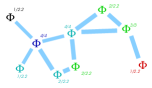
Figure 4: Example calculation of the $\hat{\Phi}_{\textup{T}}$ performance metric. For this 9-agent swarm, with accurate links indicated with thick light blue lines, the “just connected” ER expected number of links per agent is $\log(9)\simeq 2.2$; thus when working out the link-count normalisation we use this value even if the actual number of accurate links is 0, 1, or 2. Summing the contribution from each agent we get $(1+1+2+2+2+1)/2.2~{}+~{}(1+1+1)=7.1$, for a swarm performance measure of $\hat{\Phi}_{\textup{T}}\simeq 7.1/9=0.79$.

This “maximum of” is used as a pragmatic way to counteract misleading cases where an agent has (or agents have) too few beliefs that are sufficiently accurate to suggest any swarm connectivity, but where those that are accurate are nevertheless well above threshold, and so would otherwise return a misleadingly high performance measure.

Thus this thresholded agent performance measure $\bar{\Phi}^{a}_{\textup{T}}$ is

$$\bar{\Phi}^{a}_{\textup{T}} =\frac{1}{\bar{N}^{a}}\sum_{j}{\Phi}^{a}_{j}~{}H({\Phi}^{a}_{j}-{\Phi}_{\textup{T}}),$$ (13)

and by extension the corresponding swarm performance measure is

$$\hat{\Phi}_{\textup{T}} =\frac{1}{N}\sum_{i}\bar{\Phi}^{i}\quad=\frac{1}{N}\sum_{i}\frac{1}{\bar{N}^{i}}\sum_{j}{\Phi}^{a}_{j}H({\Phi}^{a}_{j}-{{\Phi}_{\textup{T}}}).$$ (14)

An example calculation is indicated on fig. 4.

Note that for any performance measure, whilst an agent $a$ might calculate (or estimate) its own performance $\bar{\Phi}^{a}$, it cannot calculate the swarm performance $\hat{\Phi}$.

As an aside, for any single set of link efficiencies $\{{L}_{ij}\}$, we could compute a customised performance scheme that uses information about what actual links are good, as opposed to the approaches introduced above where we attempted a reasonable and general normalisation. However, since an agent is never aware of the true values of $\{{L}_{ij}\}$, such a custom performance measure is not calculable by an agent attempting to determine whether it has sufficient good information about a sufficient number of nearby others. Nevertheless, such an omniscient measure could still be used as a benchmark for comparing other agent performance measures.

IV.3 Connectedness

A “completely connected swarm” (CCS) is formed if it is possible to send a message from any one agent to any other agent, possibly via intermediate agents. Here, this determination is also subject to there being (a) no more than three such hops, and (b) that the probability of the message successfully traversing the whole path is above some suitably chosen probability threshold ${\Phi}_{\textup{T}}$; as indicated on fig. 5. Here we typically choose ${\Phi}_{\textup{T}}=0.75$ and three hops, as convenient criteria that provide representative results, and making CCS connectivity achievable, but not always guaranteed. This is a different measure than the large connected component of standard network theory, but is chosen to mimic plausible limitations on message passing across the swarm. That is, this choice of ${\Phi}_{\textup{T}}=0.75$ is chosen so as to cover scenarios where some message loss is present, but where messages are not routinely lost. Increasing the value of ${\Phi}_{\textup{T}}$ demands more reliable messaging, and makes it harder to achieve the CCS criteria; decreasing it makes it easier; but in general the results are not particularly sensitive to any specific choice.

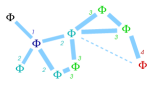
Figure 5: Counting the number of hops needed to pass a message from one agent to another. Here accurate links are indicated by the thick light blue lines, and these links are also assumed to be able to pass messages efficiently. In the situation shown here, although most agents are easily within three hops of one another, the two on the left and right extremes are four hops away from each other. Thus this swarm does not satisfy the CCS criteria, but it would if the dashed link were also accurately known. However, since it is the cumulative probability that counts for connectivity, many hop paths taken over imperfectly accurate links will in combination be less accurate (being the product of each hop accuracy), and may fall below the CCS criteria for being connected.

This determination of connectedness does make the artificial assumption that the complete set of accuracies ${\Phi}^{i}_{j}$ could somehow be collected together, to enable a matrix of agent-to-agent message success probabilities. Thus, whilst a useful metric for judging the success of a simulation or some chosen messaging tactics, it is not something that any one agent can calculate.

Indeed, in this simple model here we have that each agent $a$ is only aware of its own star-network; it has no way of inferring anything about connected components that involve hopping along multiple links. Any non-star “connected component” is not something an agent can ever be aware of, and therefore is not something an agent can use to make decisions. This is why we introduced the agent-centric performance measures $\bar{\Phi}^{i}$ above, since these tell us whether each agent is likely to have enough accurately linked neighbours in its star, so that a CCS (or even a large connected component) might exist.

Further, we do not include the effect of the link efficiencies ${L}_{ij}$, because here agents are always unaware of their values, and they are not estimated either. Clearly, this lack might be problematic, but if the ${L}_{ij}$ all have values either near 1 or 0, the ${\Phi}^{i}_{j}$ should also tend to these values, so the discrepancy should be manageable.

IV.4 Risk

The rate $\bar{R}^{a}$ that risk accumulates to any agent $a$ in this model is most simply assumed to be in proportion to a sum over its transmission rates ${\alpha}^{a}_{j}$. I.e., we have

$$\bar{R}^{a} =\xi\sum_{j}{\alpha}^{a}_{j},$$ (15)

where $\xi$ is a proportionality constant that converts a messaging rate into the rate of detection by the adversary. As a result, we can clearly see that the maximum transmission rate $\bar{A}$ set previously then also sets a maximum risk accumulation rate (“risk rate”) of $\xi\bar{A}$. However, an agent is not required to transmit at this maximum rate, so the actual risk rate can be smaller.

For all agents (i.e. the swarm), we then have the total

$$\hat{R} =\xi\sum_{i}\bar{R}^{i}\qquad=\xi\sum_{i}\sum_{j}{\alpha}^{i}_{j}.$$ (16)

Note that for any risk measure, whilst an agent $a$ might calculate its own risk rate $\bar{R}^{a}$, it cannot calculate the swarm risk rate $\hat{R}$. Further, these risk rates are not the same as detection probabilities except in the limit where they are small, i.e. when $\ll 1$. Instead, for some risk rate $R^{\prime}$ over an interval $\tau$ we can calculate the detection probability to be

$$p =1-\exp\left(-R^{\prime}\tau\right).$$ (17)

V Discrete communications

Although many of the parameters in this model are identical to the continuum model above, our discrete communication model has stochastic transmission and reception algorithms. This communications model is one which more closely matches a realistic situation of discrete messages being sent one after another to variously selected target agents. To simulate this system we wrote and used a bespoke fortran code designed around this model and its planned extensions.

Here we assume that time passes in discrete steps (or “ticks” of duration $\tau$ each), and that in each tick each agent could at most transmit one message to any one other agent. For example, a trivial comunications tactic might be to select the target agent $b$ at random from the list of other agents. This discrete communications model is very different to the continuum model which sends a continuous trickle of information to multiple other agents simultaneously.

Simulation parameters are set so that each agent sends a maximum of one message per tick, but over any period of $K$ ticks, we set the goal of sending $N$ messages. This goal of sending at a rate $A^{*}=N/\tau K$ is the counterpart of the “$\bar{A}$” parameter from the continuum model. Note that we need $K>N$ to ensure that the maximum allowed messaging rate can be maintained, although a greater margin is preferable so that we can neglect the possibilty of congestion effects. The message rate is reduced from its 1-per-tick maximum by applying conditions which need to be met before any message is sent, as we describe later in Sec. V.2.

For reception, the link efficiency ${L}_{ab}$ and the sender’s available information ${\Phi}^{a}_{b}$ can be used as a probabilistic filter to determine whether a message was received. If luck is on the receiver’s side, the message arrives successfully and it gets all the information; if not, then it gets none.

V.1 Updates (dynamics)

The resulting update equations for a tick of length $\tau$ can now be separated into two stages. For the loss update we alter each agent $a$’s information vector ${\Phi}^{a}_{j}$ according to

$${\Phi}^{a}_{j} \leftarrow{\Phi_{\textup{m}}}+\exp\left(-\gamma\tau\right)\left({\Phi}^{a}_{j}-{\Phi_{\textup{m}}}\right),$$ (18)

and for the communications stage we update according to

$${\Phi}^{a}_{j} \leftarrow{\Phi}^{a}_{j}+W^{j}_{a}.\left(1-{\Phi}^{a}_{j}\right),$$ (19)

where in any one tick, the $W^{j}_{a}$ is essentially a yes-or-no (i.e. 1 or 0) list of all successful receptions at $a$ of a (possible) transmission from all $j$. It is useful to split this $W^{j}_{a}$ into two parts, with $W^{j}_{a}=w^{j}_{a}b^{j}_{a}$, where $w^{j}_{a}$ and $b^{j}_{a}$ are defined next.

The first part ($w^{j}_{a}$) contains a “1” only if any agent $j$ transmissions sends a message to target $a$. Note that for any sending agent $b$, only the entry for the message’s intended target $a$ in $w^{b}_{i}$ is non-zero (i.e. $w^{b}_{i}=0$, except for $i=a$, since $w^{b}_{a}=1$). Which agent is chosen as a target in any given tick is now dependent on the chosen communications tactic (see below in Sec. V.2), and the (average) probability with which an agent $a$ is chosen as a target by $j$ is – for small probabilities – related to the quantity $\tau{\alpha}^{j}_{a}$ from the continuum model.

The second part ($b^{j}_{a}$) is the reception filter, which will only be non-zero (i.e. unity) if the transmission is successfully received. i.e. if some random number $\eta^{j}_{a}$ chosen from a uniform distribution on $[0,1]$ is such that $\eta^{j}_{a}<{L}_{ja}{\Phi}^{j}_{a}$.

This means that in any given tick, $W^{j}_{i}=w^{j}_{i}b^{j}_{i}$ will be mostly zeroes, and have at most $N$ entries that are one, and then only all $N$ if each sent transmission is lucky enough to successfully pass the reception filter. So here we see that unlike the continuum model’s gradual handling of information arrival and accumulation, in each tick here only some information elements are updated, and if they are updated, they are updated to become perfectly accurate beliefs, i.e. if $a$ receives from $b$, then it sets ${\Phi}^{a}_{b}=1$.

Regarding the normalisation, performance, and risk considerations present for the continuum model, here we have that:

1. The normalisation needed in the discrete model is more complicated than in the continuum model, where we could just set a maximum rate $\bar{A}$, i.e. just $\bar{A}\tau$ messages per tick. In the discrete model there is an absolute maximum for each agent of at most one message per tick, but as described above we usually want to send fewer than this, and so set a goal of (at most) $A^{*}$, i.e. $N$ messages per time $\tau K$. Thus the relevant comparison is between the continuum model’s $\bar{A}$ and the discrete model’s goal of $A^{*}$.

2. The performance measure(s) defined for our continuum model can be reused here, since they only depend on ${\Phi}^{i}_{j}$. However, since we now need to run large ensembles of instances of this model, we are not restricted to only considering only one outcome, or an averaged behaviour, of the ${\Phi}^{i}_{j}$ and values derived from it. We can also consider their distributions as accumulated over both time intervals and the many different instances.

3. The risk measure(s) defined for our continuum model can be reused here, but here they reduce to a simple message counting. To go beyond this requires both a signalling model and an adversary model to be specified (e.g. see [28]).

V.2 Communication tactics

In this discrete communications approach, we can no longer message all other agents at once, but can only send a message to one target at a time. This situation immediately suggests the simple tactic of targetting each agent sequentially, i.e. one-by-one in some fixed order; but other simple schemes are possible, most notably just choosing targets at random. More complicated tactics could involve choosing targets based on what messages were received and their timings. Any agent $a$, however, will need to consider the balance between the average number of messsages sent to other agents $i$ per tick (the counterpart of $\tau{\alpha}^{a}_{i}$ from the continuum model) and the belief decay rate ($\gamma$), and its effect on the performance of the other agents.

In the continuum case, each agent is aware of its transmission rates ${\alpha}^{a}_{i}$ and the receive rates ${q}^{a}_{j}$. Here, in analogy, agent $a$ is aware of (i) $\mathscr{T}^{a}_{j}$, how many ticks ago they last sent a message to the agent $j$, and (ii) $\mathscr{R}^{a}_{j}$, how many ticks ago they last received a message from the agent $j$. Further, each transmitted message contains the sender’s matching receive-from time, so that a messaging there-and-back “round-trip” $\mathscr{O}^{a}_{j}$ time can be calculated.

Although there is a large range of possible communications tactics, here we will restrict ourselves to a short list, three of which are closely related. We aim to address more sophisticated tactics in future work. The communications tactics we consider ensure that the messages of a sending agent are directed

1. towards each other agent in a fixed and repeating Sequence;

2. towards another agent chosen at Random;

3. towards another agent chosen at random, as long as a Timer threshold has been exceeded;

4. towards another agent chosen at random, as long as a Timer threshold has been exceeded; except if that target agent has not reported sufficiently recent contact from the sender (Filtered);

5. as per Filtered, but with an extra probability of a small number sent towards another agent chosen at random (Filtered+, Filtered++). Filtered+ incorporates a 25% chance of considering such an extra message, whilst Filtered++ has 50%.

The first three tactics here – i.e. (i), (ii), (iii) – do not attempt to select or deselect targets except as a rate-management technique; even inefficient or unreliable links will continue to be used. Although this does make them robust to unexpected changes in link efficiency, it also means they will waste messages and increase risk unnecessarily by transmitting over inefficient links. Nevertheless, they provide a set of baseline cases which we should be able to outperform.

The Filtered tactic (iv) proposed here adapts to the environment by excluding poor links. Its key feature is that it does this without requiring inferences about ${\Phi}^{a}_{i}$ or ${L}_{ai}$ values. Only timing data is needed, and for a proposed message from sending agent $a$ to target agent $b$, the only non-trivial requirement is that the last message from $b$ received by $a$ included the time $\mathscr{R}^{b}_{a}$. This tactic, and its derivatives, are the only ones considered here that will on average send fewer messages than the goal rate $A^{*}$, as excluded messaging possibilities are not redirected elsewhere, but dropped. However, once links have been deemed bad and dropped, they will never be recovered by this Filtered tactic. This is why we also introduce the Filtered+ and Filtered++ tactics (v) which – as we will see – delay this process.

VI Results: static environment

We now evaluate the performance of our chosen communications tactics using the discrete communications approach. We do not model the continuum version, since its “continually transmit to everyone, always” approach is unlikely to be of much practical use; even if it did serve a useful function in presenting some basic concepts.

Here we will consider a swarm of $N=20$ agents and contrast the cases of an in-principle fully-connectable swarm (i.e. where all ${L}_{ij}\sim 1$) and a partially-connectable swarm where ${L}_{ij}$ is a mix of zeroes and ones. The “hit by chance” minimum message targetting probability ${\Phi_{\textup{m}}}=0.10$, which, if imagining a set of spatially distributed agents, is compatible with a directed transmissions covering an angle of $36^{\circ}$. However, in this model these messages are only ever received by their intended recipient, or they are not received at all. Messages are never received accidentally by some other (non-targetted) agent, which might happen in a true spatial description [28, 33].

Each simulation run starts with randomly chosen transmitted-to and received-from communications timings, thus setting up a plausible initial state. Nevertheless, since this is not guaranteed to be a good match to a typical quasi-steady state, we start by propagating for over 10 thousand (10k) ticks so that the distribution of agent properties should no longer be dependent on the initial conditions, and the evolution can be reasonably assumed to be ergodic. Then the next $\sim 20$k ticks are averaged over in lieu of averaging over multiple independent simulations.

VI.1 Fully connectable swarm

In a fully connectable swarm, every agent has a good chance of transmitting successfully to each other agent, i.e. ${L}_{ij}\sim 1$. This makes it easy to successfully achieve a large, all-agent connected component, but there will likewise be a large number of good – but unnecessary – links that an agent might think worth maintaining.

Specifically, we consider a “flat” environment where ${L}_{ij}=0.95$, i.e. that there is only a small efficiency loss, and there are no preferred (or excluded) agent-to-agent links. Since all links are (initially) allowed for use by any of the communications tactics, and links are equally efficient, all-averaged measures – e.g. averaged ${\Phi}^{a}_{b}$ or averaged functions thereof are useful as a test of performance.

Figure 6: Filled contour plot based on histograms of the occurence-frequency of binned values of ${\Phi}^{i}_{j}$ and as a function of $\bar{\gamma}=\gamma\tau K$. Other parameters are $N=20$, $K=200$, ${\Phi_{\textup{m}}}=0.10$, with all ${L}_{ij}=0.95$. Each simulation, for the resulting agent-independent ${\alpha}^{i}_{j}=\alpha$, produces one histogram that makes up one vertical slice of the whole figure panel; thus we can scan the figure left-to-right and see how the behaviour will change as this loss ratio is increased. Here the color-coding, where dark stands for more likely, is based on the cube root of the occurence-frequencies so as to improve feature visibility. On the left, we see the results using the Random tactic (ii); and on the right, the Timer tactic (iii). The results for the Sequential tactic (i) are very similar to those for Timer (iii).

Fig. 6 shows a transition from a “good swarm” with much high-probability and accurate agent beliefs, and, as the normalised decay rate increases, changing to a fragmented (non) swarm with only the floor probability ${\Phi_{\textup{m}}}$ remaining. There is a transition region where the swarm starts to fail, where the accuracy values of ${\Phi}^{a}_{b}$ are more widely distributed. Here we see that the Timer tactic performs better than the Random one, as the frequency of high-value ${\Phi}^{i}_{j}$ is better.

In fig. 7 we see that in terms of swarm performance, the Random communications tactic is typically the worst. We should expect this, since some links will, by chance, and albeit temporarily, be neglected by an agent, leading to its accuracy dropping further. In contrast, the Timer and Sequence tactics are more regular in messaging over links, leading to a more compact distribution of accuracies (see fig. 6), and higher values (fig. 7). However, all three tactics have a similar risk profile because they are subject to the same rate limiting, and do not ignore any link posssibilities.

The results for the Filtered tactic here are only indicative, and not strictly in a quasi-steady state. This is because this tactic chooses to prohibit sending on some links, but will never re-enable them, so that even good links will – in principle – eventually have a sufficiently unlucky period that results in them being switched off. An all-links switch-off can be seen at about 30k ticks into the simulation, but only at extremely high losses $\bar{\gamma}>0.45$, is still in-progress for $0.23<\bar{\gamma}<0.45$, but not yet evident for $\bar{\gamma}<0.23$. The Filtered+ and Filtered++ tactics, with their additional random message targets, significantly delay this process, but do not entirely stop it.

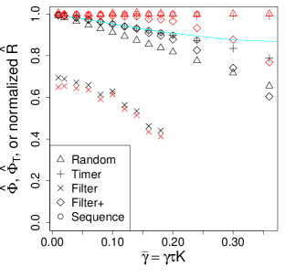
Figure 7: Comparisons of performance in both $\hat{\Phi}(1)$ (black symbols) and normalised risk $\hat{R}$ (red symbols) for the four (five) communications tactics. The “missing” $\times,\circ$ points at high $\bar{\gamma}$ are omitted for cases where no CCS was formed. The cyan line is that for the $\hat{\Phi}_{\textup{T}}$ measure, which in this plot is nearly the same for every tactic. Note that $\bar{\gamma}$ is the counterpart of $r$ in the continuum model.

VI.2 Partially connectable swarm

Next we consider a partially connectable swarm, i.e. we choose an environment where ${L}_{ij}$ is randomly chosen to be either zero or one, forming a swarm of agents that are connected to only a few neigbours, but which are connected enough so that they can in principle still be globally connected. Here we generate the same random network for each different loss value tested, with a link probability of $p=0.284$, and one instance of the resulting connectivity can be seen in fig. 8. The idea here was to ensure that the swarm was better connected than a “just connected” ER network with $p=\log(N)/N$, which for $N=20$ gives $p\simeq 0.150$, so that there are some redundant links, but not too many. This boost in link probability also helps improve connectivity, since at $N=20$ we are not in the large $N$ limit where the ER criteria is valid.

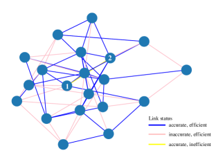
Figure 8: Background environmental network as defined by ${L}_{ij}$, shown with link colours indicating the final simulation state of a simulation with a relatively large loss $\bar{\gamma}=0.24$, and using the Filter+ tactic. Blue lines are links that are both efficient (environmental) and that are known accurately, whereas the light pink ones are efficient but inaccurately known (i.e. “lost” links”); the partly obscured yellow line is an inefficient link between agents $1$ and $2$ that by luck has unexpectedly become accurate. Although each agent in this diagram is indeed linked to each other agent via intermediate agents, for some of those paths more than three hops are required, and so a CCS is not present here.

Fig. 9 show transitions away from a “good swarm” with much high-probability and accurate agent beliefs, through to a fragmented (non) swarm with only the floor probability ${\Phi_{\textup{m}}}$ remaining. Compared to fig. 6, the good swarm regime persists for a smaller range of information decay strengths, as might be expected given the much reduced number of efficient links.

Since only a fraction of the ${L}_{ij}$ are non-zero, the simple performance measure ${\hat{\Phi}}$ is low, because it reflects this fraction – accuracies cannot be maintained if update messages never arrive. In contrast, the thresholded performance measure ${\hat{\Phi}}_{\textup{T}}$ remains high as “good links” can easily persist, although in fig. 10 we can see this drop off for higher losses. A key feature showing differences here is the normalised risk measure $\bar{R}$. For the Random, Timer, and Sequence tactics it is the same (at $\sim 1$), as expected since these tactics all send messages at the same average rate, regardless of efficiencies or accuracies. In contrast, the Filtered tactics exhibit much reduced risks, although the variants with extra “top up” messages are more risky, as would be expected.

Figure 9: Filled contour plot based on histograms of the occurence-frequency of binned values of ${\Phi}^{i}_{j}$ and as a function of rate ratio $\bar{\gamma}=\gamma\tau K$. Other parameters are $N=20$, $K=200$, ${\Phi_{\textup{m}}}=0.00$, with the ${L}_{ij}$ being randomly 0 or 1 as described in the main text. Each simulation, for some $\bar{\gamma}$, produces one histogram that makes up one vertical slice of the whole figure panel; thus we can scan the figure left-to-right and see how the behaviour will change as loss is increased. Here the color-coding, where dark stands for more likely, is based on the cube root of the occurence-frequencies so as to improve feature visibility. On the left, we see results using the Random tactic (ii), and on the right, the Filtered tactic (iii). The results for Timer and Sequential tactics are very similar to Filtered, but with better high $\bar{\gamma}$ performance.

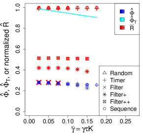
Figure 10: Comparisons of performance in both $\hat{\Phi}(1)$ (blue symbols) and scaled risk $\hat{R}$ (red symbols) for the four (five) communications tactics. The “missing” points at higher $\bar{\gamma}=\gamma\tau K$ are omitted for cases where no CCS was formed. The cyan line(s) are those for the $\hat{\Phi}_{\textup{T}}$ measure, which in this case are nearly the same for every tactic, and here are the most relevant metric for swarm performance.

On fig. 10 we see that the “all links” performance measure $\hat{\Phi}$ is uniformly low, being approximately the same as the link probability used to generate the ${L}_{ij}$; which implies that efficient links– as might be expected – lead to agents having high accuracy ${\Phi}$ values on those links. This is confirmed by the thresholded performance measure $\hat{\Phi}_{\textup{T}}$, which remains high, because it depends only on accurate belief values.

It should be noted again that although a useful steady state limit for the Random, Timer, and Sequence tactics is possible, in the long term the Filtered tactics will all gradually lose even good links to bad luck, as seen on fig. 11. Thus on fig. 10, the Filtered-type results are only indicative of a medium term performance. Nevertheless, the beneficial risk minimisation of these Filtered tactics can be maintained, e.g. by simply stopping the removal of filtered links after some suitable multiple of $K$ ticks, or perhaps setting a minimum number of links for any agent.

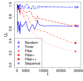
Figure 11: Swarm-averaged relative link counts $U_{r}$ as a function of simulation tick-count $t$ for the different messaging tactics. $U_{r}$ is the number of found accurate links (as determined by ${\Phi}^{i}_{j}>{\Phi}_{\textup{T}}$), divided by the total number of efficient links (as determined from ${L}_{ij}>{\Phi}_{\textup{T}}$). We see that Random, Timer, and Sequential find steady state values, but as time passes the Filtered tactics, if not stopped, lose the use of more and more links. These results are for a relatively high loss of $r=\bar{\gamma}=\gamma\tau K=0.20$, selected to emphasise the different behaviors, but are much less extreme for smaller $\bar{\gamma}$ values. Note that $\bar{\gamma}$ is the counterpart of $r$ in the continuum model.

VII Discussion

The preceeding results have shown simple scoping and initial results for our scenario considering agent-swarm management under stringent communications constraint. In particular, we have:

1. developed a simple agent information model allowing both a continuum and discrete communications paradigm; as well as a way of selecting some inter-agent communications links that are preferential (more efficient) for use than others, thus mimicking the effect of a spatial distribution of agents without extra complications.

2. discussed the need for a distinction between the contents of the model (in particular ${\Phi}^{i}_{j}$, $\gamma$, ${L}_{ij}$) and what quantities an agent $a$ should be allowed to use when taking action (e.g. not any of ${L}_{ij}$).

3. presented some metrics, notably those related to communications performance (i.e. $\hat{\Phi}$ and $\hat{\Phi}_{\textup{T}}$) and risk ($\hat{R}$) that can be used to evaluate both aspects of this performance-under-contraint scenario.

4. proposed a simple “round trip time ” test that agents can use to deprecate messaging over inefficient links ${L}_{ij}$, and which relies only on explicitly agent-knowable timing data (i.e. the Filter, Filter+, and Filter++ communications tactics).

We showed that the Filter tactics did reduce the usage of inefficent links without significantly affecting performance, at least in the medium term, and that simple modification (i.e. Filter+ and Filter++) can greatly moderate the long time failure of the unmodifed Filter tactic. Although not addressed in this initial study, which is only intended to introduce the problem, modifications to these tactics could not only stop the long term failure, but would e.g. enhance responsiveness to changes in the environment ${L}_{ij}$. Nevertheless, this double-edge behaviour from the Filter tactics does act a salutary warning that such tactics need to be checked for possible failure modes as well as for their adaptability.

It is important to note that here we have attempted as far as possible to use performance measures that are calculated in ways that only depend on agent properties, and then preferably on properties that an agent is aware of, in combination with plausible threshold parameters. This is deliberate, because agents need metrics based only on what they are aware of; and since the (e.g.) ${L_{ij}}$ are explicitly unknowns, they should not be used. Nevertheless, because our information model is so abstract, we can only judge whether an agent thinks the $a\leftrightarrow b$ link is accurate by using ${\Phi}^{a}_{b}$ regardless. However, we can still assume the results of such shortcuts based on ${\Phi}^{a}_{b}$ values are somehow representative of a comparable judgement an agent might make based on an actual basket of data containing locations and uncertainties. Only in fig. 11 do we have recourse to non-agent properties, but that is simply a normalization based on thresholded ${L_{ij}}$ values, to estimate to what extent the swarm might have accurate information about the efficient links that are present.

VIII Conclusion

Here we have considered an abstract implementation of agent-swarm behaviour in terms of a mathematical multi-agent model. We presented a simple continuum communications model which allowed some analytic treatment, but mainly focussed on a discrete communications version with a stochastic implementation which more accurately reflected any likely implementation. In particular, the stochastic version also provides us with information about outcome distributions as well as average- behaviour; something the continuum model does not generate.

We can see how these distributions are key to understanding the success/failure threshold of the swarm as seen in figs. 6 and 9. Whilst in the clear-success and clear-failure regimes (i.e. either low-loss or high-loss) the distribution of information available to the agents is indeed narrowly peaked, we see that in the transition region it broadens asymmetrically. This behaviour is key since we consider scenarios where we must operate our swarm on minimal communications, and it is somewhere in this transition region that we would aim to position our operating parameters – i.e. with enough messaging to ensure swarm coherence, but only just enough, so that risk of detection remains at a minimum.

Although the distributions in performance are key to a detailed understanding, we also used summary metrics, notably the swarm risk $\hat{R}$ and the thresholded performance measure $\hat{\Phi}_{\textup{T}}$. By thresholding, we enable the metric to ignore intrinsically inefficient and unecessary links, which should indeed be irrelevant to any practical performance measure. Further, as part of the thresholding we normalised on the basis of a minimal ER network structure, so that poorly linked agents were still penalised in the metric, but in a way not dependent on any information specific to a particular set of ${L}_{ij}$. One improvement that could be made here is to replace this minimum ER criterion with one specific to spatially distributed agents, rather than probabilistically linked ones.

Finally, the model used here was highly abstracted and not strictly applicable to any realistic agent-swarm implementation. Nevertheless, we have here proposed an interesting and novel scenario with distinctive features, and presented results and conclusions to aid in its understanding. Since the lessons exhibited here will provide useful background for more complicated scenarios and implementations, we have accordingly developed our simulation software further, allowing more sophisticated modelling [33].

Appendix: The continuum model steady state

We can normalise the dynamical equation by scaling with respect to $\gamma$, so that with $s=\gamma t$, we have a dynamical equation for any accuracy, which is

$$\frac{d}{ds}{\Phi}^{a}_{b} =-\left({\Phi}^{a}_{b}-{\Phi_{\textup{m}}}\right)+\frac{{\alpha}^{b}_{a}{L}_{ba}}{\gamma}{\Phi}^{b}_{a}\left(1-{\Phi}^{a}_{b}\right)$$ (20)

$$=-\left({\Phi}^{a}_{b}-{\Phi_{\textup{m}}}\right)+\frac{1}{R_{ab}}{\Phi}^{b}_{a}\left(1-{\Phi}^{a}_{b}\right),$$ (21)

where $R_{ab}=\gamma/{\alpha}^{b}_{a}{L}_{ba}$.

Thus the steady state un-normalised (& normalised) accuracy ${\Phi}^{a}_{b}$ is

$${\Phi}^{a}_{b} =\frac{\gamma{\Phi_{\textup{m}}}+{\alpha}^{b}_{a}{L}_{ba}{\Phi}^{b}_{a}}{\gamma+{\alpha}^{b}_{a}{L}_{ba}{\Phi}^{b}_{a}}\quad=\frac{{\Phi_{\textup{m}}}+R_{ab}^{-1}{\Phi}^{b}_{a}}{1+R_{ab}^{-1}{\Phi}^{b}_{a}},$$ (22)

and we can substitute either of these expressions into itself (with with reversed $a,b$ indices), to get a polynomial for ${\Phi}^{a}_{b}$.

We create a forward loss rate $r=\gamma/{\alpha}^{b}_{a}{L}_{ba}$ and a backward rate $r^{\prime}=\gamma/{\alpha}^{a}_{b}{L}_{ab}$, so that we have

$${\Phi}^{a}_{b} =\frac{r{\Phi_{\textup{m}}}+{\Phi}^{b}_{a}}{r+{\Phi}^{b}_{a}}$$ (23)

$$=\frac{r{\Phi_{\textup{m}}}+\frac{r^{\prime}{\Phi_{\textup{m}}}+{\Phi}^{a}_{b}}{r^{\prime}+{\Phi}^{a}_{b}}}{r+\frac{r^{\prime}{\Phi_{\textup{m}}}+{\Phi}^{a}_{b}}{r^{\prime}+{\Phi}^{a}_{b}}}$$ (24)

$${\Phi}^{a}_{b}\left\{{r\left[r^{\prime}+{\Phi}^{a}_{b}\right]+\left[r^{\prime}{\Phi_{\textup{m}}}+{\Phi}^{a}_{b}\right]}\right\} =r{\Phi_{\textup{m}}}\left[r^{\prime}+{\Phi}^{a}_{b}\right]+\left[r^{\prime}{\Phi_{\textup{m}}}+{\Phi}^{a}_{b}\right]$$ (25)

$$r^{\prime}\left[r+{\Phi_{\textup{m}}}\right]{\Phi}^{a}_{b}+\left[r+1\right]\left[{\Phi}^{a}_{b}\right]^{2} =r^{\prime}{\Phi_{\textup{m}}}\left[r+1\right]+\left[r{\Phi_{\textup{m}}}+1\right]{\Phi}^{a}_{b}$$ (26)

$$\left[r^{\prime}r+\left(r^{\prime}-r\right){\Phi_{\textup{m}}}\right]{\Phi}^{a}_{b}+\left[r+1\right]\left[{\Phi}^{a}_{b}\right]^{2} =r^{\prime}{\Phi_{\textup{m}}}\left[r+1\right]+{\Phi}^{a}_{b}.$$ (27)

Hence

$$\left[r+1\right]\left[{\Phi}^{a}_{b}\right]^{2}+\left[r^{\prime}r+\left(r^{\prime}-r\right){\Phi_{\textup{m}}}-1\right]{\Phi}^{a}_{b}-r^{\prime}{\Phi_{\textup{m}}}\left[r+1\right] =0$$ (28)

And if $r=r^{\prime}$, which would be reasonable for a symmetric environment ${L}_{ab}={L}_{ba}$, where both agent $a$ and $b$ were transmitting at the same default rate, we have the simpler form

$$\left[{\Phi}^{a}_{b}\right]^{2}+\left[r-1\right]{\Phi}^{a}_{b}-r{\Phi_{\textup{m}}} =0,$$ (29)

an expression which has just two free parameters, the rate ratio $r$ and the minimum information ${\Phi_{\textup{m}}}$.

Thus

$${\Phi}^{a}_{b} =\frac{1-r}{2}\pm\frac{1}{2}\sqrt{r^{2}-2r+1-4(-r).{\Phi_{\textup{m}}}},$$ (30)

$$=\frac{1}{2}-\frac{r}{2}\pm\frac{1}{2}\sqrt{r^{2}-2r\left(1-2{\Phi_{\textup{m}}}\right)+1}.$$ (31)

If ${\Phi_{\textup{m}}}=0$, then

$${\Phi}^{a}_{b} =\frac{1}{2}-\frac{r}{2}\pm\frac{1}{2}\left(r-1\right),$$ (32)

which has two solutions; firstly the zero accuracy case ${\Phi}^{a}_{b}=0$, and secondly the finite-accuracy case ${\Phi}^{a}_{b}=1-r$. However, if ${\Phi_{\textup{m}}}>0$, the “zero accuracy” solution (sign choice “$+$”) is pushed negative so that only the finite-accuracy one remains.