Unbounded Gradients in Federated Leaning with Buffered Asynchronous Aggregation

Abstract

Synchronous updates may compromise the efficiency of cross-device federated learning once the number of active clients increases. The FedBuff algorithm (Nguyen et al. [1]) alleviates this problem by allowing asynchronous updates (staleness), which enhances the scalability of training while preserving privacy via secure aggregation. We revisit the FedBuff algorithm for asynchronous federated learning and extend the existing analysis by removing the boundedness assumptions from the gradient norm. This paper presents a theoretical analysis of the convergence rate of this algorithm when heterogeneity in data, batch size, and delay are considered.

I Introduction

Federated learning (FL) is an approach in machine learning theory and practice that allows training models on distributed data sources [2, 3]. The distributed structure of FL has numerous benefits over traditional centralized methods, including parallel computing, efficient storage, and improvements in data privacy. However, this framework also presents communication efficiency, data heterogeneity, and scalability challenges. Several works have been proposed to improve the performance of FL [4, 5, 6]. Existing works usually address a subset of these challenges while imposing additional constraints or limitations in other aspects. For example, the work in [7] shows a trade-off between privacy, communication efficiency, and accuracy gains for the distributed discrete Gaussian mechanism for FL with secure aggregation.

One of the most important advantages of FL is scalability. Training models on centralized data stored on a single server can be problematic when dealing with large amounts of data. Servers may be unable to handle the load, or clients might refuse to share their data with a third party. In FL, the data is distributed across many devices, potentially improving data privacy and computation scalability. However, this also presents some challenges. First, keeping the update mechanism synchronized across all devices may be very difficult when the number of clients is large [8]. Second, even if feasible, imposing synchronization results in huge (unnecessary) delays in the learning procedure [6]. Finally, each client often might have different data distributions, which can impact the convergence of algorithms [9, 10].

In synchronous FL, e.g., FedAvg [3, 2], the server first sends a copy of the current model to each client. The clients then train the model locally on their private data and send the model updates back to the server. The server then aggregates the client updates to produce a new shared model. The process is repeated for many rounds until the shared model converges to the desired accuracy. However, the existence of delays, message losses, and stragglers hinders the performance of distributed learning. Several works have been proposed to improve the scalability of federated/distributed learning via enabling asynchronous communications [11, 12, 8, 13, 6, 14, 15]. In the majority of these results, each client immediately communicates the parameters to the server after applying a series of local updates. The server updates the global parameter once it receives any client update. This has the benefit of reducing the training time and better scalability in practice and theory [16, 6, 12, 15] since the server can start aggregating the client updates as soon as they are available.

The setup, known as “vanilla” asynchronous FL, has several challenges that must be addressed. First, due to the nature of asynchronous updates, the clients are supposed to deal with staleness, where the client updates are not up-to-date with the current model on the server [1]. Moreover, the asynchronous setup may imply potential risks for privacy due to the lack of secure aggregation, i.e., the immediate communication of every single client to the server [17, 18]. In [1], the authors proposed an algorithm called federated learning with buffered asynchronous aggregation (FedBuff), which modifies pure asynchronous FL by enabling secure aggregation while clients perform asynchronous updates. This novel method is considered a variant of asynchronous FL while serving as an intermediate approach between synchronous and asynchronous FL.

TABLE I: Comparison of the characteristics considered in our analysis with relevant works for federated learning for smooth & non-convex objective functions. Parameter $\tau$ denotes the maximum delay.

Algorithm	Reference	Asynchronous	Buffered	Unbounded	Convergence
		Update	Aggregation	Gradient	Rate
	McMahan et al. [2]	✗	✓	-	-
FedAvg	Yu et al. [19]	✗	✓	✗	$\mathcal{O}\left(\frac{1}{\sqrt{T}}\right)$
	Wang et al. [10]	✗	✓	✓	$\mathcal{O}\left(\frac{1}{\sqrt{T}}\right)$
FedAsync	Xie et al. [8]	✓	✗	✗	$\mathcal{O}\left(\frac{1}{\sqrt{T}}\right)+\mathcal{O}\left(\frac{\tau^{2}}{T}\right)$
FedBuff	Nguyen et al. [1]	✓	✓	✗	$\mathcal{O}\left(\frac{1}{\sqrt{T}}\right)+\mathcal{O}\left(\frac{\tau^{2}}{T}\right)$
	This Work	✓	✓	✓	$\mathcal{O}\left(\frac{1}{\sqrt{T}}\right)+\mathcal{O}\left(\frac{\tau^{2}}{T}\right)$

FedBuff [1] is shown to converge for the class of smooth and non-convex objective functions under the boundedness of the gradient norm. By removing this assumption, we provide a new analysis for FedBuff and improve the existing theory by extending it to a broader class of functions. We derive our bounds based on stochastic and heterogeneous variance and the maximum delay between downloads and uploads across all the clients. Table I summarizes the properties and rate of our analysis for FedBuff algorithm alongside and provides a comparison with existing analyses for FedAsync [8] and FedAvg [3, 2]. The rates reflect the complexity of the number of updates performed by the central server. The speed of asynchronous algorithms is faster since the constraint for synchronized updates is removed in asynchronous variations. To our knowledge, this is the first analysis for (a variant of) asynchronous federated learning with no boundedness assumption on the gradient norm.

Following is an outline of the remainder of this paper. The problem setup and FedBuff algorithm are presented in Section II. Moreover, our convergence result and its corresponding assumptions are provided in Section II. We state detailed proof of our result in section III. Finally, we conclude remarks and prospects for future research in Section IV.

II Problem Setup, Algorithm, & Main Result

In this section, we first state the problem setup, and after explaining the FedBuff algorithm [1], we present our main result along with the underlying assumptions.

$\diamond$ Problem Setup: We consider a set of $n$ clients and one server, where each client $i\in[n]$ owns a private function $f_{i}:\mathbb{R}^{d}\to\mathbb{R}$ and the goal is to jointly minimize the average local cost functions via finding a $d$-dimensional parameter $w\in\mathbb{R}^{d}$ that

$$\begin{split}\min_{w\in\mathbb{R}^{d}}f(w)&\coloneqq\frac{1}{n}\sum\limits_{i=1}^{n}f_{i}(w),\\ \text{with}\quad f_{i}(w)&\coloneqq\mathbb{E}_{\xi_{i}\sim p_{i}}[\ell_{i}(w,\xi_{i})],\end{split}$$ (1)

where $\ell_{i}:\mathbb{R}^{d}\times\mathcal{S}_{i}\to\mathbb{R}$ is a cost function that determines the prediction error of $w$ over a single data point $\xi_{i}\in\mathcal{S}_{i}$ on user $i$, and $p_{i}$ represents user $i$’s data distribution over $\mathcal{S}_{i}$, for $i\in[n]$. In the above definition, $f_{i}(\cdot)$ is the local cost function of client $i$, and $f(\cdot)$ denotes the global (average) cost function which the clients try to collaboratively minimize. Now, let $\mathcal{D}_{i}$ be a data batch sampled from $p_{i}$. Similar to (1), we denote the stochastic cost function $\tilde{f}_{i}(w,\mathcal{D}_{i})$ as follows:

$$\tilde{f}_{i}(w,\mathcal{D}_{i}) \coloneqq\frac{1}{|\mathcal{D}_{i}|}\sum\limits_{\xi_{i}\in\mathcal{D}_{i}}\ell_{i}(w,\xi_{i}).$$ (2)

Minimization of (1) by having access to an oracle of samples and its variants are extensively studied for many different frameworks [4]. Now, we are ready to explain the FedBuff.

$\diamond$ FedBuff Algorithm: Let $w^{0}$ be the initialization parameter at the server. The ultimate goal is to minimize the cost function in (1), using an algorithm via access to the stochastic gradients. All clients can communicate with the server, and each client $i\in[n]$ communicates when its connection to the server is stable. First, let us explain the FedBuff algorithm from the client and server perspectives.

1. Client Algorithm: Each client $i$ requests to read the server’s parameter $w\in\mathbb{R}^{d}$ once the connection is stable and the server is ready to send the parameter. There is often some delay in this step which we call the download delay. This may be originated from factors such as unstable connection, bandwidth limit, or communication failure. For example, maybe the server seeks to reduce the simultaneously active users by setting client $i$ on hold. The download delay can model all these factors. Once the parameter is received (downloaded) from the server, client $i$ performs $Q$ steps of local stochastic gradient descent starting from the downloaded model $w$ for its cost function $f_{i}(\cdot)$. In words, agent $i$ runs a $Q$-step algorithm (loop of size $Q$), where at each local round $q\in\{0,1,\dots Q{-}1\}$, client $i$ samples a data batch $\mathcal{D}_{i,q}$ with respect to distribution $p_{i}$ and performs one step of gradient descent with local stepsize $\eta>0$. Finally, agent $i$ returns the updates (the difference between the initial and final parameters) to the server. We refer to the time required to broadcast parameters to the server as the upload delay, which could have similar factors as the download delay. Agent repeats all this procedure until the server sends a termination message. Algorithm 1 summarizes the pseudo-code of operations at client $i\in[n]$, where Steps 4-8 show the local updates performed at the agent. Moreover, $\Delta_{i}$ in Step 9 denotes the difference communicated to the server.

   Algorithm 1 FedBuff (Client $i$)

   1:  input: number of local steps $Q$, local stepsize $\eta$.

   2:  repeat

   3:     read $w$ from the server {download phase}

   4:     $w_{i,0}\leftarrow w$

   5:     for $q=0$ to $Q{-}1$ do

   6:        sample a data batch $\mathcal{D}_{i,q}$

   7:         $w_{i,q+1}\leftarrow w_{i,q}-\eta\nabla\tilde{f}_{i}(w_{i,q},\mathcal{D}_{i,q})$

   8:     end for

   9:     $\Delta_{i}\leftarrow w_{i,0}-w_{i,Q}$

   10:     client $i$ broadcasts $\Delta_{i}$ to the server{upload phase}

   11:  until not interrupted by the server

2. Server Algorithm: The server considers an initialization for parameter $w^{0}\in\mathbb{R}^{d}$. Then, starting from timestep $t=0$, the server repeats an iterative procedure in addition to sending its parameters to the clients upon their request. Algorithm 2 describes the server operations in FedBuff. In a nutshell, the algorithm consists of two parts, (i) secure aggregation of client updates in a buffer with size $K\geq 1$, and (ii) update the parameters using the aggregated updates. In other words, let $k,t$ respectively denote the indices associated with buffer and server updates. The server starting from $t=0$, receives updates broadcast by the agents asynchronously depending on their upload & download delays as well as the time required for $Q$ local updates. A secure buffered aggregates these updates, up to $K$ separate updates received by the clients in $\overline{\Delta}^{0}$, initially set to zero. By indexing $k$, we keep track of uploaded updates on the server. When the buffer saturates of $K$ different updates, the server uses the aggregator parameter $\overline{\Delta}^{0}$ and updates its parameter $w^{0}$ according to line 9 of Algorithm 2. Then, the server increases its update counter $t$ and removes all updates from the buffer, i.e., $k=0$. In this algorithm, we denote the agent which sends the $k$-th update at round $t$ by index $i_{t,k}\in[n]$. Basically, server repeats Steps 5-14 until some convergence criteria be satisfied. After the convergence, the server sends a termination message to all the clients.

As we described above, the crucial novelty of this algorithm is on the server side, where the server operations, with the help of a secure buffered aggregation, control the staleness and prevent unnecessary access to individual updates. Note that for $K=1$, the presented algorithm reduces to vanilla asynchronous federated learning with no buffer aggregation. Figure 1 illustrates the update schedule for FedBuff and provides a comparison with the asynchronous updates in FedAvg [2]. As shown on the left of Figure 1, the vertical lines with light blue color are associated with uploaded updates. Note that the buffer size is $K=2$ in this example. These vertical lines are of two types, (i) solid or (ii) hatched. The solid lines reflect the time the buffer is full, so the server performs an update. Contrary to FedBuff, under the synchronous updates (as shown in the right figure), the server should halt the training procedure until all clients selected within one round receive the updates.

Algorithm 2 FedBuff (Server)

1:  input: model $w^{0}$, server stepsize $\beta$, buffer size $K$

2:  $t\leftarrow 0$, $k\leftarrow 0$

3:  $\overline{\Delta}^{0}\leftarrow 0$

4:  repeat

5:     if the server receives an update $\Delta_{i_{t,k}}$ from some client $i_{t,k}{\in}[n]$ then

6:        $\overline{\Delta}^{t}\leftarrow\overline{\Delta}^{t}+\Delta_{i_{t,k}}$

7:        $k\leftarrow k+1$

8:        if $k=K$ then

9:           $w^{t+1}\leftarrow w^{t}-\beta\overline{\Delta}^{t}$

10:           $k\leftarrow 0$

11:           $t\leftarrow t+1$

12:           $\overline{\Delta}^{t}\leftarrow 0$

13:        end if

14:     end if

15:  until not converged

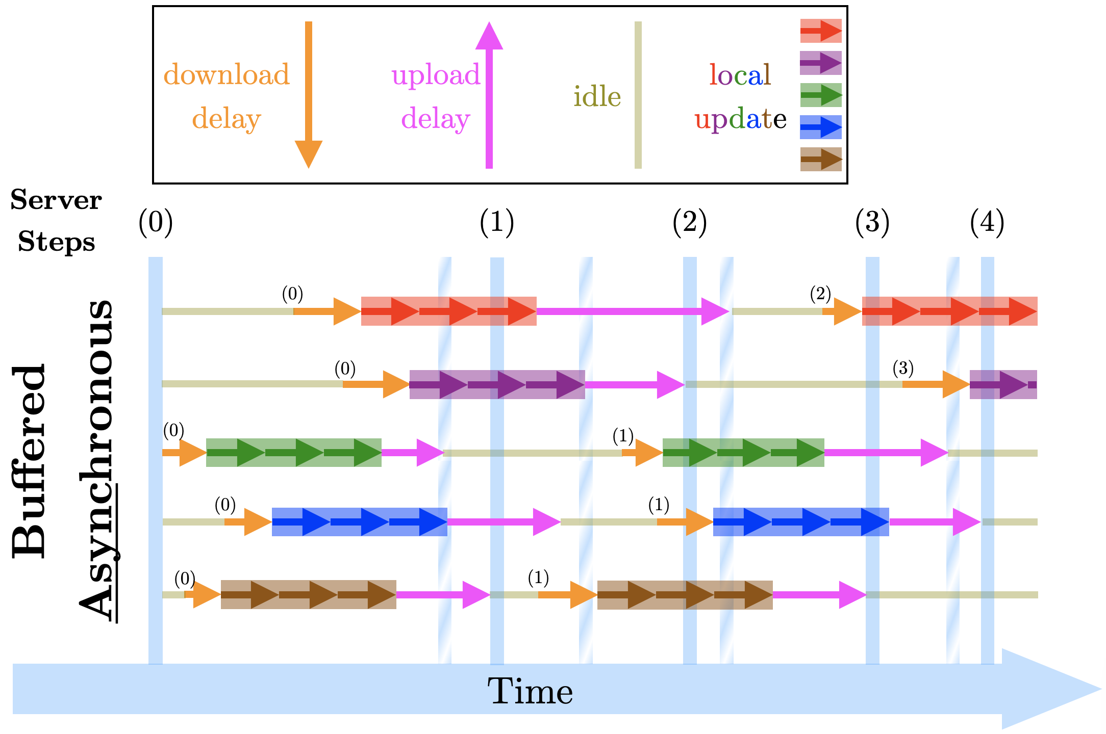
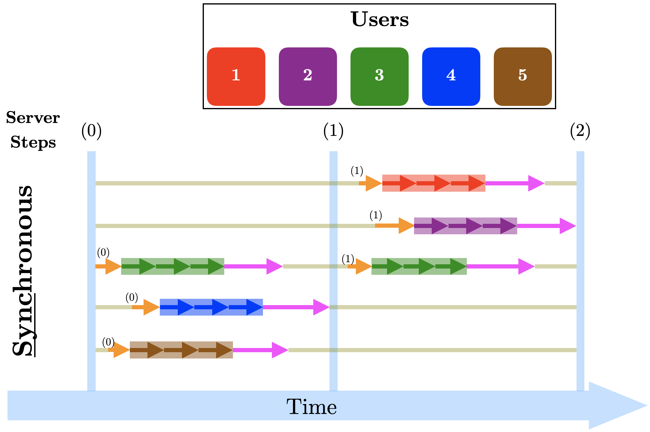
Figure 1: Communication and update schedule for synchronous and buffered asynchronous aggregation: The demonstrated setup in this example contains $n=5$ agents, with $Q=3$ local updates, buffer size $K=2$ for FedBuff [1], and sampling rate $0.6$ for FedAvg [2].

Next, we present our assumptions on staleness, bounded stochasticity, and population diversity (heterogeneity).

$\diamond$ Assumptions & Main Result: Here, we present our main result alongside a few standard assumptions. First, to be coherent with the proof in [1], let us denote $\tau_{i}^{t}$ to be the timestep of the last downloaded parameter on client $i\in[n]$ up to the $t$-th update at the server. We are ready to introduce the assumptions in our analysis for FedBuff, i.e., Algorithms 1 & 2.

Assumption 1 (Bounded Staleness).

For all clients, $i\in[n]$ and server steps $t\geq 0$, the staleness or effective delay between the download and upload steps is bounded by some constant $\tau$, i.e.,

$$\sup_{t\geq 0}\max_{i\in[n]}\left\lvert t-\tau_{i}^{t}\right\rvert\leq\tau,$$ (3)

and the server receives updates uniformly, i.e., $i_{t,k}\sim\mathrm{Uniform}([n])$.

Note that $\tau_{i}^{t}$ is the timestep of the last parameter downloaded via agent $i$ up to timestep $t$ at the server. Therefore, if agent $i$ contributes in the $(t{+}1)$-th update, i.e., $i_{t,k}=i$, for some $k\in\{0,1,\dots,K{-}1\}$, the difference between the download and upload rounds is bounded. This is a standard assumption in the analysis of asynchronous algorithms with heterogeneous data on the clients.

Assumption 2 (Smoothness).

For all clients $i\in[n]$, function $f_{i}:\mathbb{R}^{d}\to\mathbb{R}$ is bounded below, differentiable, and $L$-smooth, i.e., for all $w,u\in\mathbb{R}^{d}$,

$$\left\lVert\nabla f_{i}(w)-\nabla f_{i}(u)\right\rVert\leq L\lVert w-u\rVert$$ (4)

$$f_{i}^{\star}\coloneqq\min_{w\in\mathbb{R}^{d}}f_{i}(w)>-\infty.$$ (5)

This assumption guarantees the necessary conditions for analyzing smooth & non-convex functions. Note that boundedness from below can be relaxed only to the global cost function $f$, i.e., it is sufficient to only assume that $f^{\star}\coloneqq\min_{w\in\mathbb{R}^{d}}f(w)>-\infty$ in our analysis instead of (5) for all $i\in[n]$. Now, we introduce the assumptions on bounded stochasticity and heterogeneity.

Assumption 3 (Bounded Variance).

For all clients $i\in[n]$, the variance of a stochastic gradient $\nabla\ell_{i}(w,\xi_{i})$ on a single data point $\xi_{i}\in\mathcal{S}_{i}$ is bounded, i.e., for all $w\in\mathbb{R}^{d}$

$$\mathbb{E}_{\xi_{i}\sim p_{i}}\left\lVert\nabla\ell_{i}(w,\xi_{i})-\nabla f_{i}(w)\right\rVert^{2}\leq\sigma^{2}.$$ (6)

This assumption is conventional in the analysis of stochastic optimization algorithms and has been used in many relevant works [20, 1, 6, 9, 10, 21, 14]. Note that as we defined the stochastic loss in (2) and used the stochastic gradients in Step 7, we also need to show the stochastic variance for the gradients of the sampled batches. For simplicity, let us assume that all batch sizes are of size at least $b$, therefore according to (6), we have:

$$\mathbb{E}_{p_{i}}\left\lVert\nabla\tilde{f}_{i}(w,\mathcal{D}_{i})-\nabla f_{i}(w)\right\rVert^{2}\leq\frac{\sigma^{2}}{|\mathcal{D}_{i}|}\leq\hat{\sigma}^{2}\coloneqq\frac{\sigma^{2}}{b}.$$ (7)

Assumption 4 (Bounded Population Diversity).

For all $w\in\mathbb{R}^{d}$, the gradients of local functions $f_{i}(w)$ and the global function $f(w)$ satisfy the following property:

$$\frac{1}{n}\sum\limits_{i=1}^{n}\lVert\nabla f_{i}(w)-\nabla f(w)\rVert^{2}\leq\gamma^{2}.$$ (8)

In our analysis, we work with heterogeneous cost functions. Therefore, it is a reasonable and conventional assumption to assume that the boundedness of the population diversity [1, 22, 5]. The inequality in 9 measures the variance of local full gradients from the average full gradient, which resembles to the expressions in (6) & (7). The authors of [5] discusses the connection of this bound to the similarity of local data distributions $p_{i}$, for all $i\in[n]$.

Now, we present our result under the stated assumptions.

Theorem 1.

Let Assumptions 1-4 hold, $\beta=\frac{1}{K}$, and $\eta=\frac{1}{Q\sqrt{LT}}$. Then, the following property holds for the joint iterates of Algorithms 1 and 2: for any timestep $T\geq 160L(Q{+}7)(\tau{+}1)^{3}$ at the server

$$\frac{1}{T}\sum_{t=0}^{T-1}\,\mathbb{E}\left\lVert\nabla f\left(w^{t}\right)\right\rVert^{2} \leq\frac{8\sqrt{L}\left(f(w^{0}){-}f^{\star}\right)}{\sqrt{T}}$$

$$+\frac{16\sqrt{L}\left(\frac{\sigma^{2}}{b}+\gamma^{2}\right)}{\sqrt{T}}$$

$$+\frac{320L(Q{+}1)(\tau^{2}{+}1)\left(\frac{\sigma^{2}}{b}+n\gamma^{2}\right)}{T}.$$

We present the proof for Theorem 1 in Section III.

The above theorem states the convergence of the FedBuff algorithm to a first-order stationary point. This result states a convergence rate of $\mathcal{O}\left(\frac{1}{\sqrt{T}}\right)+\mathcal{O}\left(\frac{\tau^{2}}{T}\right)$, where the term affected by the maximum delay (second term) decays faster, hence the same convergence complexity as the synchronized counterpart. Note that this rate states the number of updates occurring on the server (iteration complexity), which in the case of asynchronous updates, practically converges much faster ($3.3\times$ according to [1]) than synchronized updates.

Remark 1.

The choice of $\beta$ in Theorem 1 is an arbitrary option that implies the rate in the theorem statement. The convergence proof holds for any choices of $\beta$, such that $\beta K=\mathcal{O}\left(1\right)$.

Remark 2.

In our analysis for Theorem 1, we considered bounded population diversity in Assumption 4. One can see that by relaxing this assumption to a stronger variant

$$\max_{i\in[n]}\sup_{w\in\mathbb{R}^{d}}\lVert\nabla f_{i}(w)-\nabla f(w)\rVert^{2}\leq\gamma^{2},$$ (9)

i.e., uniformly bounded heterogeneity, $n\gamma^{2}$ can be replaced with $\gamma^{2}$ in the third term of the rate.

Next, we will provide detailed proof for Theorem 1.

III Convergence Result

This section provides a detailed explanation of the proof of the convergence result in Section II.

Proof of Theorem 1.

Before proceeding with the proof, let us state some inequalities. For any set of $m$ vectors $\{w_{i}\}_{i{=}1}^{m}$ such that $w_{i}\in\mathbb{R}^{d}$, and a constant $\alpha>0$, the following properties hold: for all $i,j\in[m]$:

$$\lVert w_{i}+w_{j}\rVert^{2} \leq(1{+}\alpha)\lVert w_{i}\rVert^{2}+(1{+}\alpha^{-1})\lVert w_{j}\rVert^{2},$$ (10a)

$$2\langle w_{i},w_{j}\rangle \leq\alpha\lVert w_{i}\rVert^{2}+\alpha^{-1}\lVert w_{j}\rVert^{2},$$ (10b)

$$\left\lVert\sum\limits_{i=1}^{m}w_{i}\right\rVert^{2} \leq m\left(\sum\limits_{i=1}^{m}\lVert w_{i}\rVert^{2}\right).$$ (10c)

For simplicity, let us denote $\tilde{\nabla}f_{i}\left(w\right)=\nabla\tilde{f}_{i}\left(w,\mathcal{D}_{i}\right)$. Therefore, at round $t$, the server updates its parameter by receiving $\overline{\Delta}^{t}$, as follows:

$$w^{t{+}1} =w^{t}-\beta\overline{\Delta}^{t}=w^{t}-\beta\sum_{k=0}^{K{-}1}\Delta_{i_{t,k}}$$

$$=w^{t}-\eta\beta\sum_{k=0}^{K{-}1}\sum\limits_{q=0}^{Q{-}1}\tilde{\nabla}f_{i_{t,k}}\left(w_{i_{t,k},q}^{\tau_{i_{t,k}}^{t}}\right).$$ (11)

Due to Assumption 2, we can infer that $f$ is $L$-smooth, thus

$$f(w^{t{+}1} )\overset{\eqref{eq:smoothness}}{\leq}f(w^{t})+\frac{L\eta^{2}\beta^{2}}{2}\underbrace{\left\lVert\sum_{k=0}^{K{-}1}\sum\limits_{q=0}^{Q{-}1}\tilde{\nabla}f_{i_{t,k}}\left(w_{i_{t,k},q}^{\tau_{i_{t,k}}^{t}}\right)\right\rVert^{2}}_{=:S_{1}}$$

$$+\eta\beta\underbrace{\left\langle\nabla f(w^{t}),\sum_{k=0}^{K{-}1}\sum\limits_{q=0}^{Q{-}1}\tilde{\nabla}f_{i_{t,k}}\left(w_{i_{t,k},q}^{\tau_{i_{t,k}}^{t}}\right)\right\rangle}_{=:S_{2}}$$ (12)

We first provide a lower bound on term $S_{2}$ in (III). Let us denote $\tilde{g}_{i}^{t}=\sum_{q{=}0}^{Q{-}1}\tilde{\nabla}f_{i}(w_{i,q}^{\tau_{i}^{t}})$, $\tilde{g}^{t}=\frac{1}{n}\sum_{i{=}1}^{n}\tilde{g}_{i}^{t}$, $g_{i}^{t}=\sum_{q{=}0}^{Q{-}1}\nabla f_{i}(w_{i,q}^{\tau_{i}^{t}})$, and $g^{t}=\frac{1}{n}\sum_{i{=}1}^{n}g_{i}^{t}$. Therefore,

$$\mathbb{E}\left[S_{2}\right]=\mathbb{E}\left[\mathbb{E}_{i_{t,k}}\left\langle\nabla f(w^{t}),\sum_{k=0}^{K{-}1}\sum\limits_{q=0}^{Q{-}1}\tilde{\nabla}f_{i_{t,k}}\left(w_{i_{t,k},q}^{\tau_{i_{t,k}}^{t}}\right)\right\rangle\right]$$

$$=\mathbb{E}\left\langle\nabla f(w^{t}),\frac{1}{n}\sum\limits_{i=1}^{n}\sum_{k=0}^{K{-}1}\mathbb{E}_{p_{i}}\left[\tilde{g}_{i}^{t}\right]\right\rangle$$ (13)

$$=KQ\,\mathbb{E}\left\lVert\nabla f(w^{t})\right\rVert^{2}+K\left[\mathbb{E}\left\langle\nabla f(w^{t}),g^{t}-Q\nabla f(w^{t})\right\rangle\right]$$

$${\geq}\frac{K(2Q{-}1)}{2}\,\mathbb{E}\left\lVert\nabla f(w^{t})\right\rVert^{2}-\frac{K}{2}\mathbb{E}\left\lVert g^{t}-Q\nabla f(w^{t})\right\rVert^{2}.$$

Moreover, the following holds for $S_{1}$ in (III):

$$\mathbb{E}\left[S_{1}\right] =\mathbb{E}\left[\mathbb{E}_{i_{t,k}}\left\lVert\sum_{k=0}^{K{-}1}\sum\limits_{q=0}^{Q{-}1}\tilde{\nabla}f_{i_{t,k}}\left(w_{i_{t,k},q}^{\tau_{i_{t,k}}^{t}}\right)\right\rVert^{2}\right]$$

$$=\frac{1}{n}\mathbb{E}\left[\sum\limits_{i=1}^{n}\left\lVert\sum_{k=0}^{K{-}1}\sum\limits_{q=0}^{Q{-}1}\tilde{\nabla}f_{i}\left(w_{i,q}^{\tau_{i}^{t}}\right)\right\rVert^{2}\right]$$ (14)

$$=\frac{K^{2}}{n}\,\sum\limits_{i=1}^{n}\mathbb{E}\left\lVert\sum\limits_{q=0}^{Q{-}1}\tilde{\nabla}f_{i}\left(w_{i,q}^{\tau_{i}^{t}}\right)\right\rVert^{2}=\frac{K^{2}}{n}\,\sum\limits_{i=1}^{n}\mathbb{E}\left\lVert\tilde{g}_{i}^{t}\right\rVert^{2}.$$

Now, according to (III), (III), and (III), we have:

$$\mathbb{E}f\left(w^{t{+}1}\right)\leq\mathbb{E}f(w^{t})-\frac{\eta\beta K(2Q{-}1)}{2}\mathbb{E}\left\lVert\nabla f(w^{t})\right\rVert^{2}$$ (15)

$$+\frac{\eta\beta K}{2}\mathbb{E}\underbrace{\left\lVert g^{t}-Q\nabla f(w^{t})\right\rVert^{2}}_{=:S_{3}}+\frac{L\eta^{2}\beta^{2}K^{2}}{2n}\mathbb{E}\underbrace{\left[\sum\limits_{i=1}^{n}\left\lVert\tilde{g}_{i}^{t}\right\rVert^{2}\right]}_{=:S_{4}},$$

where we bound $S_{3},S_{4}$ as follows:

$$S_{3} =\left\lVert\frac{1}{n}\sum\limits_{i=1}^{n}\left(g_{i}^{t}-Q\nabla f_{i}(w^{t})\right)\right\rVert^{2}$$

$${\leq}\frac{1}{n}\sum\limits_{i=1}^{n}\left\lVert g_{i}^{t}-Q\nabla f_{i}(w^{t})\right\rVert^{2}$$

$$=\frac{1}{n}\sum\limits_{i=1}^{n}\left\lVert\sum\limits_{q{=}0}^{Q{-}1}\left[\nabla f_{i}\left(w_{i,q}^{\tau_{i}^{t}}\right)-\nabla f_{i}(w^{t})\right]\right\rVert^{2}$$

$${\leq}\frac{Q}{n}\sum\limits_{i=1}^{n}\sum\limits_{q=0}^{Q{-}1}\left\lVert\nabla f_{i}\left(w_{i,q}^{\tau_{i}^{t}}\right)-\nabla f_{i}(w^{t})\right\rVert^{2},$$ (16)

and

$$S_{4} =\sum\limits_{i=1}^{n}\Big{\lVert}\sum\limits_{q{=}0}^{Q{-}1}\tilde{\nabla}f_{i}\left(w_{i,q}^{\tau_{i}^{t}}\right)\Big{\rVert}^{2}$$

$${\leq}Q\sum\limits_{i=1}^{n}\sum\limits_{q{=}0}^{Q{-}1}\Big{\lVert}\tilde{\nabla}f_{i}\left(w_{i,q}^{\tau_{i}^{t}}\right)\Big{\rVert}^{2}$$

$$=Q\sum\limits_{i=1}^{n}\sum\limits_{q{=}0}^{Q{-}1}\Big{\lVert}\tilde{\nabla}f_{i}\left(w_{i,q}^{\tau_{i}^{t}}\right)-\nabla f_{i}\left(w_{i,q}^{\tau_{i}^{t}}\right)$$

$$+\nabla f_{i}\left(w_{i,q}^{\tau_{i}^{t}}\right)-\nabla f_{i}\left(w^{t}\right)$$

$$+\nabla f_{i}\left(w^{t}\right)-\nabla f\left(w^{t}\right)+\nabla f\left(w^{t}\right)\Big{\rVert}^{2}$$

$${\leq}4Q\sum\limits_{i=1}^{n}\sum\limits_{q{=}0}^{Q{-}1}\Bigg{[}\Big{\lVert}\tilde{\nabla}f_{i}\left(w_{i,q}^{\tau_{i}^{t}}\right)-\nabla f_{i}\left(w_{i,q}^{\tau_{i}^{t}}\right)\Big{\rVert}^{2}$$

$$+\Big{\lVert}\nabla f_{i}\left(w_{i,q}^{\tau_{i}^{t}}\right)-\nabla f_{i}\left(w^{t}\right)\Big{\rVert}^{2}$$

$$+\Big{\lVert}\nabla f_{i}\left(w^{t}\right)-\nabla f\left(w^{t}\right)\Big{\rVert}^{2}+\Big{\lVert}\nabla f\left(w^{t}\right)\Big{\rVert}^{2}\Bigg{]},$$ (17)

therefore, by taking expectations, we can show that:

$$\mathbb{E}[S_{4}] {\leq}4nQ^{2}\left[\hat{\sigma}^{2}+\gamma^{2}+\mathbb{E}\Big{\lVert}\nabla f\left(w^{t}\right)\Big{\rVert}^{2}\right]$$

$$+4Q\sum\limits_{i=1}^{n}\sum\limits_{q{=}0}^{Q{-}1}\mathbb{E}\left\lVert\nabla f_{i}\left(w_{i,q}^{\tau_{i}^{t}}\right)-\nabla f_{i}(w^{t})\right\rVert^{2}.$$ (18)

Therefore, due to (15)-(III), we have

$$\mathbb{E} f\left(w^{t{+}1}\right)\leq\mathbb{E}f(w^{t})$$

$$-\left[\frac{\eta\beta K(2Q{-}1)}{2}-2\eta^{2}L\beta^{2}K^{2}Q^{2}\right]\mathbb{E}\left\lVert\nabla f(w^{t})\right\rVert^{2}$$

$$+\frac{\eta\beta KQ}{2n}\sum\limits_{i=1}^{n}\sum\limits_{q{=}0}^{Q{-}1}\mathbb{E}\left\lVert\nabla f_{i}\left(w_{i,q}^{\tau_{i}^{t}}\right)-\nabla f_{i}(w^{t})\right\rVert^{2}$$

$$+\frac{2\eta^{2}\beta^{2}K^{2}QL}{n}\sum\limits_{i=1}^{n}\sum\limits_{q{=}0}^{Q{-}1}\mathbb{E}\left\lVert\nabla f_{i}\left(w_{i,q}^{\tau_{i}^{t}}\right)-\nabla f_{i}(w^{t})\right\rVert^{2}$$

$$+2\eta^{2}L\beta^{2}K^{2}Q^{2}\hat{\sigma}^{2}+2\eta^{2}L\beta^{2}K^{2}Q^{2}\gamma^{2}$$

$${\leq}\mathbb{E}f(w^{t})$$

$$-\left[\frac{\eta\beta K(2Q{-}1)}{2}-2\eta^{2}L\beta^{2}K^{2}Q^{2}\right]\mathbb{E}\left\lVert\nabla f(w^{t})\right\rVert^{2}$$

$$+\frac{\eta\beta KQL^{2}\left(1{+}4\eta\beta KL\right)}{2n}\sum\limits_{i=1}^{n}\sum\limits_{q{=}0}^{Q{-}1}\mathbb{E}\underbrace{\left\lVert w_{i,q}^{\tau_{i}^{t}}-w^{t}\right\rVert^{2}}_{=:S_{5}}$$

$$+2\eta^{2}L\beta^{2}K^{2}Q^{2}\hat{\sigma}^{2}+2\eta^{2}L\beta^{2}K^{2}Q^{2}\gamma^{2}.$$ (19)

Hence, it is sufficient to bound $S_{5}$ in (III) as follows:

$$S_{5} =\left\lVert w^{t}-w_{i,q}^{\tau_{i}^{t}}\right\rVert^{2}=\left\lVert\sum\limits_{s{=}\tau_{i}^{t}}^{t{-}1}\left(w^{s{+}1}-w^{s}\right)+w^{\tau_{i}^{t}}-w_{i,q}^{\tau_{i}^{t}}\right\rVert^{2}$$

$${\leq}\left(1{+}\frac{1}{\beta^{2}K^{2}}\right)\left\lVert\sum\limits_{s{=}\tau_{i}^{t}}^{t{-}1}\left(w^{s{+}1}-w^{s}\right)\right\rVert^{2}$$

$$+\quad\left(1{+}\beta^{2}K^{2}\right)\left\lVert w^{\tau_{i}^{t}}-w_{i,q}^{\tau_{i}^{t}}\right\rVert^{2}$$

$${\leq}\tau\left(1{+}\frac{1}{\beta^{2}K^{2}}\right)\left[\sum\limits_{s{=}t{-}\tau}^{t{-}1}\underbrace{\left\lVert w^{s{+}1}-w^{s}\right\rVert^{2}}_{=:S_{7}}\right]$$

$$+\qquad\left(1{+}\beta^{2}K^{2}\right)\underbrace{\left\lVert w^{\tau_{i}^{t}}-w_{i,q}^{\tau_{i}^{t}}\right\rVert^{2}}_{=:S_{6}}.$$ (20)

Now, we show a bound on the evolution of local updates at an arbitrary round $s\geq 0$, i.e., the distance between $w_{i,q}^{s}$ and $w^{s}$, which we will use to provide a bound on $S_{7}$.

$$\mathbb{E}\left\lVert w_{i,q}^{s}-w^{s}\right\rVert^{2}=\mathbb{E}\left\lVert w_{i,q{-}1}^{s}-\eta\tilde{\nabla}f_{i}\left(w_{i,q{-}1}^{s}\right)-w^{s}\right\rVert^{2}$$

$$=\mathbb{E}\Big{\lVert}w_{i,q{-}1}^{s}-w^{s}-\eta\nabla f\left(w^{s}\right)$$

$$\quad-\eta\tilde{\nabla}f_{i}\left(w_{i,q{-}1}^{s}\right)+\eta\nabla f_{i}\left(w_{i,q{-}1}^{s}\right)$$

$$\quad-\eta\nabla f_{i}\left(w_{i,q{-}1}^{s}\right)+\eta\nabla f_{i}\left(w^{s}\right)$$

$$\quad-\eta\nabla f_{i}\left(w^{s}\right)+\eta\nabla f\left(w^{s}\right)\Big{\rVert}^{2}$$

$${\leq}\left(1{+}\frac{1}{2Q}\right)\mathbb{E}\Big{\lVert}w_{i,q{-}1}^{s}-w^{s}\Big{\rVert}^{2}$$

$$+\hskip 10.00002pt4(1{+}2Q)\eta^{2}\mathbb{E}\Bigg{[}\Big{\lVert}\tilde{\nabla}f_{i}\left(w_{i,q{-}1}^{s}\right)-\nabla f_{i}\left(w_{i,q{-}1}^{s}\right)\Big{\rVert}^{2}$$

$$\hskip 71.00017pt+\Big{\lVert}\nabla f_{i}\left(w_{i,q{-}1}^{s}\right)-\nabla f_{i}\left(w^{s}\right)\Big{\rVert}^{2}$$

$$\hskip 71.00017pt+\Big{\lVert}\nabla f_{i}\left(w^{s}\right)-\nabla f\left(w^{s}\right)\Big{\rVert}^{2}$$

$$\hskip 71.00017pt+\Big{\lVert}\nabla f\left(w^{s}\right)\Big{\rVert}^{2}\Bigg{]}$$ (21)

$${\leq}\left(1{+}\frac{1}{2Q}\right)\mathbb{E}\Big{\lVert}w_{i,q{-}1}^{s}-w^{s}\Big{\rVert}^{2}$$

$$+\hskip 10.00002pt4(1{+}2Q)\eta^{2}\Bigg{[}\hat{\sigma}^{2}+L^{2}\,\mathbb{E}\Big{\lVert}w_{i,q{-}1}^{s}-w^{s}\Big{\rVert}^{2}$$

$$\hskip 71.00017pt+\mathbb{E}\Big{\lVert}\nabla f_{i}\left(w^{s}\right)-\nabla f\left(w^{s}\right)\Big{\rVert}^{2}$$

$$\hskip 71.00017pt+\mathbb{E}\Big{\lVert}\nabla f\left(w^{s}\right)\Big{\rVert}^{2}\Bigg{]}.$$ (22)

Note that we can select stepsize $\eta\leq\frac{1}{4L(Q{+}1)}$ such that

$$\eta^{2}\leq\frac{1}{8L^{2}Q(2Q{+}1)}\Rightarrow 4(1+2Q)\eta^{2}L^{2}\leq\frac{1}{2Q},$$ (23)

therefore, due to (III)-(22) and (23), we have:

$$\underbrace{\mathbb{E}\left\lVert w_{i,q}^{s}-w^{s}\right\rVert^{2}}_{:=P_{i,q}^{s}}\leq\left(1{+}\frac{1}{Q}\right)\underbrace{\mathbb{E}\Big{\lVert}w_{i,q{-}1}^{s}-w^{s}\Big{\rVert}^{2}}_{:=P_{i,q{-}1}^{s}}$$

$$+4(1{+}2Q)\eta^{2}\Bigg{[}\hat{\sigma}^{2}+\mathbb{E}\Big{\lVert}\nabla f_{i}\left(w^{s}\right)-\nabla f\left(w^{s}\right)\Big{\rVert}^{2}$$

$$\underbrace{\qquad\qquad\qquad\qquad\qquad\qquad+\mathbb{E}\Big{\lVert}\nabla f\left(w^{s}\right)\Big{\rVert}^{2}\Bigg{]}}_{:=R_{i}^{s}}\Rightarrow$$ (24)

$$P_{i,q}^{s} \leq\left(1{+}\frac{1}{Q}\right)P_{i,q{-}1}^{s}+R_{i}^{s}$$

$$=R_{i}^{s}\sum\limits_{k=0}^{q{-}1}\left(1{+}\frac{1}{Q}\right)^{k}\leq R_{i}^{s}\sum\limits_{k=0}^{Q{-}1}\left(1{+}\frac{1}{Q}\right)^{k}$$

$$=R_{i}^{s}\frac{\left(1{+}\frac{1}{Q}\right)^{Q}-1}{\left(1{+}\frac{1}{Q}\right)-1}=R_{i}^{s}Q\left[\left(1{+}\frac{1}{Q}\right)^{Q}-1\right]$$

$$\leq R_{i}^{s}Q(e-1)\leq 2R_{i}^{s}Q,$$ (25)

for all $q\in[Q]$. Note that according to Algorithm 2, we have:

$$w^{s{+}1} =w^{s}-\beta\sum\limits_{k=0}^{K{-}1}\left[w^{\tau_{i_{s}}^{s}}-w_{i_{s},Q}^{\tau_{i_{s}}^{s}}\right]\Rightarrow$$ (26)

$$\mathbb{E}\left\lVert w^{s{+}1}-w^{s}\right\rVert^{2}\leq\beta^{2}\,\mathbb{E}\left\lVert\sum\limits_{k=0}^{K{-}1}\left[w^{\tau_{i_{s}}^{s}}-w_{i_{s},Q}^{\tau_{i_{s}}^{s}}\right]\right\rVert^{2}$$

$${\leq}\beta^{2}K^{2}\left[\mathbb{E}\left[\mathbb{E}_{i_{s}}\left\lVert w^{\tau_{i_{s}}^{s}}-w_{i_{s},Q}^{\tau_{i_{s}}^{s}}\right\rVert^{2}\right]\right]$$

$$=\frac{\beta^{2}K^{2}}{n}\sum\limits_{j{=}1}^{n}\mathbb{E}\left\lVert w^{\tau_{j}^{s}}-w_{j,Q}^{\tau_{j}^{s}}\right\rVert^{2}$$

$${\leq}8Q(1{+}2Q)\eta^{2}\beta^{2}K^{2}\hat{\sigma}^{2}$$

$$+\frac{8Q(1{+}2Q)\eta^{2}\beta^{2}K^{2}}{n}\sum_{j=1}^{n}\mathbb{E}\Big{\lVert}\nabla f_{j}\left(w^{\tau_{j}^{s}}\right){-}\nabla f\left(w^{\tau_{j}^{s}}\right)\Big{\rVert}^{2}$$

$$+\frac{8Q(1{+}2Q)\eta^{2}\beta^{2}K^{2}}{n}\sum_{j=1}^{n}\mathbb{E}\Big{\lVert}\nabla f\left(w^{\tau_{j}^{s}}\right)\Big{\rVert}^{2}.$$ (27)

Let $\phi=8\eta^{2}Q^{2}(1{+}2Q)(1{+}\beta^{2}K^{2})$, then according to (III)-(LABEL:eq:s7-end), we have

$$\frac{1}{n\phi}\sum_{i=1}^{n}\sum_{q=0}^{Q{-}1}\mathbb{E}[S_{5}]$$

$$\leq\tau\left[\sum\limits_{s{=}t{-}\tau}^{t{-}1}\left\lVert w^{s{+}1}-w^{s}\right\rVert^{2}\right]+\frac{1}{n}\sum_{i=1}^{n}\left\lVert w^{\tau_{i}^{t}}-w_{i,q}^{\tau_{i}^{t}}\right\rVert^{2}$$

$$\leq\tau^{2}\hat{\sigma}^{2}+\frac{\tau}{n}\sum_{s=t{-}\tau}^{t{-}1}\sum_{j=1}^{n}\mathbb{E}\Big{\lVert}\nabla f_{j}\left(w^{\tau_{j}^{s}}\right)-\nabla f\left(w^{\tau_{j}^{s}}\right)\Big{\rVert}^{2}$$

$$+\frac{\tau}{n}\sum_{s=t{-}\tau}^{t{-}1}\sum_{j=1}^{n}\mathbb{E}\Big{\lVert}\nabla f\left(w^{\tau_{j}^{s}}\right)\Big{\rVert}^{2}+\frac{1}{n}\sum_{i=1}^{n}\mathbb{E}\Big{\lVert}\nabla f\left(w^{\tau_{i}^{t}}\right)\Big{\rVert}^{2}$$

$$+\hat{\sigma}^{2}+\frac{1}{n}\sum_{i=1}^{n}\mathbb{E}\Big{\lVert}\nabla f_{i}\left(w^{\tau_{i}^{t}}\right)-\nabla f\left(w^{\tau_{i}^{t}}\right)\Big{\rVert}^{2}.$$ (28)

Note that according to (3), we know that: $\tau_{i}^{t}\in\{t{-}\tau\,\dots,t\}$, therefore:

$$\mathbb{E}\Big{\lVert}\nabla f\left(w^{\tau_{i}^{t}}\right)\Big{\rVert}^{2}\leq\sum_{s=t{-}\tau}^{t}\mathbb{E}\Big{\lVert}\nabla f\left(w^{s}\right)\Big{\rVert}^{2},$$ (29)

and similarly, for any $s\in\{t{-}\tau\,\dots,t\}$ and $j\in[n]$,

$$\mathbb{E}\Big{\lVert}\nabla f\left(w^{\tau_{j}^{s}}\right)\Big{\rVert}^{2}\leq\sum_{u=s{-}\tau}^{s}\mathbb{E}\Big{\lVert}\nabla f\left(w^{u}\right)\Big{\rVert}^{2}.$$ (30)

Moreover, we have:

$$\Big{\lVert}\nabla f_{j}\left(w^{\tau_{j}^{s}}\right) -\nabla f\left(w^{\tau_{j}^{s}}\right)\Big{\rVert}^{2}$$

$$\leq\sum_{i=1}^{n}\Big{\lVert}\nabla f_{i}\left(w^{\tau_{j}^{s}}\right)-\nabla f\left(w^{\tau_{j}^{s}}\right)\Big{\rVert}^{2}.$$ (31)

Therefore, due to (III)-(III), we have:

$$\frac{1}{n\phi}\sum_{i=1}^{n}\sum_{q=0}^{Q{-}1}\mathbb{E}[S_{5}] {\leq}\tau^{2}\hat{\sigma}^{2}+\tau^{2}n\gamma^{2}$$

$$+\tau\sum_{s=t{-}\tau}^{t{-}1}\sum_{u=s{-}\tau}^{s}\mathbb{E}\Big{\lVert}\nabla f\left(w^{u}\right)\Big{\rVert}^{2}$$

$$+\hat{\sigma}^{2}+n\gamma^{2}+\sum_{s=t{-}\tau}^{t}\mathbb{E}\Big{\lVert}\nabla f\left(w^{s}\right)\Big{\rVert}^{2}$$

$$=(1{+}\tau^{2})\left[\hat{\sigma}^{2}+n\gamma^{2}\right]$$

$$+\tau\sum_{s=t{-}\tau}^{t{-}1}\sum_{u=s{-}\tau}^{s}\mathbb{E}\Big{\lVert}\nabla f\left(w^{u}\right)\Big{\rVert}^{2}$$

$$+\sum_{s=t{-}\tau}^{t}\mathbb{E}\Big{\lVert}\nabla f\left(w^{s}\right)\Big{\rVert}^{2}.$$ (32)

By combining (III) and (III), we have the following inequality:

$$\mathbb{E}f\left(w^{t{+}1}\right)\leq\mathbb{E}f(w^{t})+2\eta^{2}L\beta^{2}K^{2}Q^{2}\left[\hat{\sigma}^{2}+\gamma^{2}\right]$$

$$-\frac{\eta\beta K}{2}\Big{[}(2Q{-}1)-4\eta L\beta KQ^{2}$$

$$\qquad\qquad-QL^{2}(1{+}\tau^{2})\left(1{+}4\eta\beta KL\right)\phi\Big{]}\mathbb{E}\left\lVert\nabla f(w^{t})\right\rVert^{2}$$

$$+\frac{\eta\beta KQL^{2}\left(1{+}4\eta\beta KL\right)\phi}{2}$$

$$\quad\qquad\sum_{s=t{-}\tau}^{t{-}1}\left[\mathbb{E}\Big{\lVert}\nabla f\left(w^{s}\right)\Big{\rVert}^{2}+\tau\sum_{u=s{-}\tau}^{s}\mathbb{E}\Big{\lVert}\nabla f\left(w^{u}\right)\Big{\rVert}^{2}\right]$$

$$+\frac{\eta\beta KQL^{2}(1{+}\tau^{2})\left(1{+}4\eta\beta KL\right)\phi}{2}\left[\hat{\sigma}^{2}+n\gamma^{2}\right]$$

$$\leq\mathbb{E}f(w^{t})+2\eta^{2}L\beta^{2}K^{2}Q^{2}\left[\hat{\sigma}^{2}+\gamma^{2}\right]$$

$$-\frac{\eta\beta KQ}{2}\Big{[}1-4\eta L\beta KQ$$

$$\qquad\qquad-QL^{2}(1{+}\tau^{2})\left(1{+}4\eta\beta KL\right)\phi\Big{]}\mathbb{E}\left\lVert\nabla f(w^{t})\right\rVert^{2}$$

$$+\frac{\eta\beta KQL^{2}\left(1{+}4\eta\beta KL\right)\phi}{2}$$

$$\quad\qquad\sum_{s=t{-}\tau}^{t{-}1}\left[\mathbb{E}\Big{\lVert}\nabla f\left(w^{s}\right)\Big{\rVert}^{2}+\tau\sum_{u=s{-}\tau}^{s}\mathbb{E}\Big{\lVert}\nabla f\left(w^{u}\right)\Big{\rVert}^{2}\right]$$

$$+\frac{\eta\beta KQL^{2}(1{+}\tau^{2})\left(1{+}4\eta\beta KL\right)\phi}{2}\left[\hat{\sigma}^{2}+n\gamma^{2}\right].$$ (33)

Now, we can obtain the following inequality by rearranging the terms in (III):

$$\big{[}1-4\eta L\beta KQ-QL^{2}(1{+}\tau^{2})\left(1{+}4\eta\beta KL\right)\phi\big{]}\mathbb{E}\left\lVert\nabla f(w^{t})\right\rVert^{2}$$

$$-L^{2}\left(1{+}4\eta\beta KL\right)\phi\sum_{s=t{-}\tau}^{t{-}1}\Big{[}\mathbb{E}\Big{\lVert}\nabla f\left(w^{s}\right)\Big{\rVert}^{2}$$

$$\qquad\qquad\qquad\qquad\qquad\quad+\tau\sum_{u=s{-}\tau}^{s}\mathbb{E}\Big{\lVert}\nabla f\left(w^{u}\right)\Big{\rVert}^{2}\Big{]}$$

$$\leq\frac{2\left[\mathbb{E}f(w^{t})-\mathbb{E}f\left(w^{t{+}1}\right)\right]}{\eta\beta KQ}+4\eta\beta KQL\left[\hat{\sigma}^{2}+\gamma^{2}\right]$$

$$+2L^{2}(1{+}\tau^{2})\left(1{+}4\eta\beta KL\right)\phi\left[\hat{\sigma}^{2}+n\gamma^{2}\right],$$ (34)

whereby mixing the terms in (III), we obtain:

$$\big{[}1-4\eta L\beta KQ-L^{2}(\tau^{2}{+}1)\left(1{+}4\eta\beta KL\right)\phi\big{]}\mathbb{E}\left\lVert\nabla f(w^{t})\right\rVert^{2}$$

$$\quad-L^{2}\left(1{+}4\eta\beta KL\right)(\tau{+}1)\phi\sum_{s=t{-}\tau}^{t{-}1}\sum_{u=s{-}\tau}^{s}\mathbb{E}\Big{\lVert}\nabla f\left(w^{u}\right)\Big{\rVert}^{2}$$

$$\leq\frac{2\left[\mathbb{E}f(w^{t})-\mathbb{E}f\left(w^{t{+}1}\right)\right]}{\eta\beta KQ}+4\eta\beta KQL\left[\hat{\sigma}^{2}+\gamma^{2}\right]$$

$$+2L^{2}(1{+}\tau^{2})\left(1{+}4\eta\beta KL\right)\phi\left[\hat{\sigma}^{2}+n\gamma^{2}\right].$$ (35)

Finally, we add (III), for $t=0,1,\dots T{-}1$, and divide by $T$ to show that:

$$\Bigg{[}1-4\eta L\beta KQ-L^{2}(\tau^{2}{+}1)\left(1{+}4\eta\beta KL\right)\phi$$

$$\qquad\qquad-L^{2}\left(1{+}4\eta\beta KL\right)\tau(\tau{+}1)^{2}\phi\Bigg{]}\frac{\sum\limits_{t=0}^{T{-}1}\mathbb{E}\left\lVert\nabla f(w^{t})\right\rVert^{2}}{T}$$

$$\leq\frac{2\left[f(w^{0})-\mathbb{E}f\left(w^{T}\right)\right]}{\eta\beta KQ}+4\eta\beta KQL\left[\hat{\sigma}^{2}+\gamma^{2}\right]$$

$$+2L^{2}(1{+}\tau^{2})\left(1{+}4\eta\beta KL\right)\phi\left[\hat{\sigma}^{2}+n\gamma^{2}\right].$$ (36)

Let us fix $\beta=\frac{1}{K}$ and $\eta=\frac{1}{Q\sqrt{LT}}$. Thus, we know that the following inequality holds

$$\max\Big{\{}4\eta\beta KLQ,\,L^{2}(\tau^{2}{+}1)(1{+}4\eta\beta KL)\phi,$$

$$\qquad\quad L^{2}\tau(\tau{+}1)^{2}(1{+}4\eta\beta KL)\phi\Big{\}} \leq\frac{1}{4},$$ (37)

for $T\geq 160L(Q{+}7)(\tau{+}1)^{3}$. Note that under this choices for $\eta$ and $\beta$, we also have $\eta\leq\frac{1}{4L(Q{+}1)}$, which we used in (23). Therefore, we can conclude the result in Theorem 1 as follows:

$$\frac{1}{T}\sum\limits_{t=0}^{T{-}1}\mathbb{E}\left\lVert\nabla f(w^{t})\right\rVert^{2} \leq\frac{8\sqrt{L}\left(f(w^{0})-\mathbb{E}f\left(w^{T}\right)\right)}{\sqrt{T}}$$

$$+\frac{16\sqrt{L}\left(\hat{\sigma}^{2}+\gamma^{2}\right)}{\sqrt{T}}$$ (38)

$$+\frac{320L(Q{+}1)(\tau^{2}{+}1)\left(\hat{\sigma}^{2}+n\gamma^{2}\right)}{T}.$$

∎

IV Conclusion

This paper studied the convergence properties of asynchronous federated learning via secure buffered aggregation. By removing the boundedness assumption on the gradient norms, we presented a novel analysis of the convergence of the FedBuff algorithm, where we showed a sublinear convergence rate of $\mathcal{O}(\epsilon^{2})+\mathcal{O}({\tau^{2}}\epsilon)$ to an $\epsilon$-first-order stationary solution. We also discussed the dependence of this rate on the batch size, stochasticity variance, data heterogeneity, and maximum delays. We leave the privacy analysis of Fed-Buff with gradient clipping and noise addition to future studies. Also, the communication complexity of this method and the extensions to decentralized setups remain for future work.

References

• [1] John Nguyen, Kshitiz Malik, Hongyuan Zhan, Ashkan Yousefpour, Mike Rabbat, Mani Malek, and Dzmitry Huba, “Federated learning with buffered asynchronous aggregation,” in International Conference on Artificial Intelligence and Statistics. PMLR, 2022, pp. 3581–3607.
• [2] Brendan McMahan, Eider Moore, Daniel Ramage, Seth Hampson, and Blaise Aguera y Arcas, “Communication-efficient learning of deep networks from decentralized data,” in Artificial intelligence and statistics. PMLR, 2017, pp. 1273–1282.
• [3] Jakub Konečnỳ, H Brendan McMahan, Felix X Yu, Peter Richtárik, Ananda Theertha Suresh, and Dave Bacon, “Federated learning: Strategies for improving communication efficiency,” arXiv preprint arXiv:1610.05492, 2016.
• [4] Peter Kairouz, H Brendan McMahan, Brendan Avent, Aurélien Bellet, Mehdi Bennis, Arjun Nitin Bhagoji, Kallista Bonawitz, Zachary Charles, Graham Cormode, Rachel Cummings, et al., “Advances and open problems in federated learning,” arXiv preprint arXiv:1912.04977, 2019.
• [5] Alireza Fallah, Aryan Mokhtari, and Asuman Ozdaglar, “Personalized federated learning with theoretical guarantees: A model-agnostic meta-learning approach,” Advances in Neural Information Processing Systems, vol. 33, 2020.
• [6] Mahmoud Assran, Arda Aytekin, Hamid Reza Feyzmahdavian, Mikael Johansson, and Michael G Rabbat, “Advances in asynchronous parallel and distributed optimization,” Proceedings of the IEEE, vol. 108, no. 11, pp. 2013–2031, 2020.
• [7] Peter Kairouz, Ziyu Liu, and Thomas Steinke, “The distributed discrete gaussian mechanism for federated learning with secure aggregation,” in International Conference on Machine Learning. PMLR, 2021, pp. 5201–5212.
• [8] Cong Xie, Sanmi Koyejo, and Indranil Gupta, “Asynchronous federated optimization,” arXiv preprint arXiv:1903.03934, 2019.
• [9] Ahmed Khaled, Konstantin Mishchenko, and Peter Richtárik, “Tighter theory for local sgd on identical and heterogeneous data,” in International Conference on Artificial Intelligence and Statistics. PMLR, 2020, pp. 4519–4529.
• [10] Jianyu Wang, Qinghua Liu, Hao Liang, Gauri Joshi, and H Vincent Poor, “Tackling the objective inconsistency problem in heterogeneous federated optimization,” Advances in neural information processing systems, vol. 33, pp. 7611–7623, 2020.
• [11] Yanan Li, Shusen Yang, Xuebin Ren, and Cong Zhao, “Asynchronous federated learning with differential privacy for edge intelligence,” arXiv preprint arXiv:1912.07902, 2019.
• [12] Hamid Reza Feyzmahdavian, Arda Aytekin, and Mikael Johansson, “An asynchronous mini-batch algorithm for regularized stochastic optimization,” IEEE Transactions on Automatic Control, vol. 61, no. 12, pp. 3740–3754, 2016.
• [13] Kenta Niwa, Guoqiang Zhang, W Bastiaan Kleijn, Noboru Harada, Hiroshi Sawada, and Akinori Fujino, “Asynchronous decentralized optimization with implicit stochastic variance reduction,” in International Conference on Machine Learning. PMLR, 2021, pp. 8195–8204.
• [14] Anastasia Koloskova, Sebastian U Stich, and Martin Jaggi, “Sharper convergence guarantees for asynchronous sgd for distributed and federated learning,” arXiv preprint arXiv:2206.08307, 2022.
• [15] Konstantin Mishchenko, Francis Bach, Mathieu Even, and Blake Woodworth, “Asynchronous sgd beats minibatch sgd under arbitrary delays,” arXiv preprint arXiv:2206.07638, 2022.
• [16] Feng Niu, Benjamin Recht, Christopher Ré, and Stephen J Wright, “Hogwild!: A lock-free approach to parallelizing stochastic gradient descent,” arXiv preprint arXiv:1106.5730, 2011.
• [17] Keith Bonawitz, Vladimir Ivanov, Ben Kreuter, Antonio Marcedone, H Brendan McMahan, Sarvar Patel, Daniel Ramage, Aaron Segal, and Karn Seth, “Practical secure aggregation for federated learning on user-held data,” arXiv preprint arXiv:1611.04482, 2016.
• [18] Wei-Ning Chen, Christopher A Choquette-Choo, and Peter Kairouz, “Communication efficient federated learning with secure aggregation and differential privacy,” in NeurIPS 2021 Workshop Privacy in Machine Learning, 2021.
• [19] Hao Yu, Sen Yang, and Shenghuo Zhu, “Parallel restarted sgd with faster convergence and less communication: Demystifying why model averaging works for deep learning,” in Proceedings of the AAAI Conference on Artificial Intelligence, 2019, vol. 33, pp. 5693–5700.
• [20] Sebastian Urban Stich, “Local sgd converges fast and communicates little,” in ICLR 2019-International Conference on Learning Representations, 2019, number CONF.
• [21] Anastasia Koloskova, Tao Lin, Sebastian U Stich, and Martin Jaggi, “Decentralized deep learning with arbitrary communication compression,” arXiv preprint arXiv:1907.09356, 2019.
• [22] Canh T Dinh, Nguyen H Tran, and Tuan Dung Nguyen, “Personalized federated learning with moreau envelopes,” arXiv preprint arXiv:2006.08848, 2020.
• [23] Jianyu Wang, Zachary Charles, Zheng Xu, Gauri Joshi, H Brendan McMahan, Maruan Al-Shedivat, Galen Andrew, Salman Avestimehr, Katharine Daly, Deepesh Data, et al., “A field guide to federated optimization,” arXiv preprint arXiv:2107.06917, 2021.