Modeling the Extragalactic Background Light and the Cosmic Star Formation History

Abstract

We present an updated model for the extragalactic background light (EBL) from stars and dust, over wavelengths $\approx 0.1\ \mu\mathrm{m}$ to $1000\ \mu\mathrm{m}$. This model uses accurate theoretical stellar spectra, and tracks the evolution of star formation, stellar mass density, metallicity, and interstellar dust extinction and emission in the universe with redshift. Dust emission components are treated self-consistently, with stellar light absorbed by dust reradiated in the infrared as three blackbody components. We fit our model, with free parameters associated with star formation rate and dust extinction and emission, to a wide variety of data: luminosity density, stellar mass density, and dust extinction data from galaxy surveys; and $\gamma$-ray absorption optical depth data from $\gamma$-ray telescopes. Our results strongly constraint the star formation rate density and dust photon escape fraction of the universe out to redshift $z=10$, about 90% of the history of the universe. We find our model result is, in some cases, below lower limits on the $z=0$ EBL intensity, and below some low-$z$ $\gamma$-ray absorption measurements.

1. Introduction

The Extragalactic Background Light (EBL) in the range $0.1-1000$ $\mu$m consists of the background light from all of the stars that have existed in the observable universe. Direct stellar emission produces a component at $\approx 0.1-4$ $\mu$m (the cosmic optical background or COB), and the absorption of starlight that is reradiated in the infrared (IR) produces a component at $\approx 4-1000$ $\mu$m (the cosmic IR background or CIB). The EBL contains a great deal of information about the star formation history of the universe and dust emission; however, it is difficult to observe directly. The night sky is dominated by emission from the atmosphere, the solar system (zodiacal light emitted by interplanetary dust mostly within the orbit of Jupiter; e.g., Wright, 2001; Rowan-Robinson & May, 2013; Korngut et al., 2022), and the Milky Way (e.g., Seon et al., 2011; Brandt & Draine, 2012; Chellew et al., 2022), all of which are brighter than the EBL. Telescopes above the atmosphere can measure the EBL without the contaminating atmospheric foreground (e.g., Hauser et al., 1998; Bernstein et al., 2002; Mattila, 2003; Bernstein, 2007), although these can still suffer from contamination from stray light from the Eath, Moon, or Sun outside the field of view of the instrument (Caddy et al., 2022). Spacecraft beyond the orbit of Jupiter have made measurements of the EBL with minimal contamination from the zodiacal light (Toller, 1983; Edelstein et al., 2000; Matsuoka et al., 2011; Zemcov et al., 2017; Lauer et al., 2021, 2022). However, there is still the difficulty of contamination from the Milky Way foreground. Galaxy number counts can give lower limits on the EBL (e.g., Madau & Pozzetti, 2000; Marsden et al., 2009; Driver et al., 2016; Koushan et al., 2021) but do not include unresolved sources.

It was realized in the 1960s that the EBL would have an effect on observed $\gamma$-ray spectra of extragalactic sources (Nikishov, 1962; Gould & Schréder, 1967a; Fazio & Stecker, 1970). The high-energy $\gamma$ rays are absorbed, producing electron positron pairs. EBL photons with wavelength $\lambda_{\rm EBL}$ will absorb $\gamma$ rays above observed energy

$$E_{\gamma}=0.22\ \left(\frac{\lambda_{\rm EBL}}{\mu{\rm m}}\right)\ \mathrm{TeV}$$ (1)

producing electron-positron pairs and absorbing the $\gamma$-ray photon (e.g., Gould & Schréder, 1967b). The cross section for this process is strongly peaked at an energy about a factor of 2 greater than the energy in Equation (1). In recent years, this has led to a number of attempts to measure the EBL with extragalactic $\gamma$-ray sources, primarily blazars, and a number of modeling efforts.

Constraints on the EBL with $\gamma$ rays have been found with ground-based imaging atmospheric telescopes (IACTs) such as MAGIC, H.E.S.S., and VERITAS; and with the Large Area Telescope (LAT) on the Fermi Gamma-ray Space Telescope in low Earth orbit. The different telescopes observe at different energies, and probe different wavelengths and redshifts ($z$) of the EBL. The IACTs are sensitive to absorption of $\sim 0.1$–$10\ \mathrm{TeV}$ $\gamma$ rays, which allows them to constrain the nearby ($z\lesssim 1$) EBL at $\lambda_{\rm EBL}\approx 0.5$—$50\ \mu$m [Equation (1)]. The LAT observes $\gamma$-ray absorption in the $10$—$100\ \mathrm{GeV}$ range ($\gamma$-rays below $\approx 10$ GeV are not absorbed) and so probes the EBL at $z\gtrsim 1$ and $\lambda_{\rm EBL}\approx 0.5$—$0.05\ \mu$m. IACT constraints on the EBL can be done with IACTs only (e.g., Aharonian et al., 1999; Protheroe & Meyer, 2000; Schroedter, 2005; Aharonian et al., 2006, 2007; Mazin & Raue, 2007; Finke & Razzaque, 2009; Orr et al., 2011; Abramowski et al., 2013; Biteau & Williams, 2015; Desai et al., 2019; Abeysekara et al., 2019; Biasuzzi et al., 2019) or extrapolating the LAT spectrum into the IACT bandpass and using this to constrain the intrinsic blazar very-high energy (VHE) $\gamma$-ray spectra (e.g., Georganopoulos et al., 2010; Meyer et al., 2012; Acciari et al., 2019); or by performing detailed multiwavelength modeling of the blazar $\gamma$-ray source to constrain the intrinsic VHE spectra (e.g., Mankuzhiyil et al., 2010; Domínguez et al., 2013). LAT constraints on the EBL have been found from blazars and gamma-ray bursts (GRBs) by Abdo et al. (2010); Ackermann et al. (2012); Desai et al. (2017); and Abdollahi et al. (2018). Besides $\gamma$-ray absorption, the EBL can create $\gamma$-rays in the LAT bandpass, by being Compton scattered by high-energy electrons in the lobes of radio galaxies. This could in principle be used to constrain the EBL through LAT observations of radio galaxies (Georganopoulos et al., 2008); however, efforts to do so have been hampered by unexpected additional $\gamma$-ray emission components from the radio lobes, possibly of hadronic origin (McKinley et al., 2015; Ackermann et al., 2016), the existence of which is controversial (Persic & Rephaeli, 2019a, b, 2020). A review of $\gamma$-ray constraints on the EBL is given by Dwek & Krennrich (2013).

Recent EBL models begin by modeling the ultraviolet (UV) through IR luminosity densities (the total luminosity per unit volume of the universe) across cosmic time; then integrating over $z$ to get the EBL intensity as a function of redshift; then integrating over the redshift between a $\gamma$-ray source and us to compute the $\gamma\gamma$ absorption optical depth (see Sections 2.9 and 2.10 below for details). Modeling the EBL and determining the model $\gamma$-ray absorption then is a matter of determining the luminosity density. The luminosity density can be determined by integrating a galaxy luminosity function, which is determined from deep surveys. Models which directly use the results of galaxy survey data to construct the EBL include the models of Franceschini et al. (2008); Domínguez et al. (2011); Helgason & Kashlinsky (2012); Stecker et al. (2012); Scully et al. (2014); Stecker et al. (2016); Franceschini & Rodighiero (2017); and Saldana-Lopez et al. (2021). Other models use the cosmic star formation rate density (SFRD), models of stellar emission, interstellar dust extinction, and dust emission to determine the luminosity density. The SFRD can be determined from various measurements of star formation, as in the models of Salamon & Stecker (1998); Kneiske et al. (2002, 2004); Razzaque et al. (2009); Finke et al. (2010); Kneiske & Dole (2010); Khaire & Srianand (2015); Andrews et al. (2018); Khaire & Srianand (2019), and Koushan et al. (2021). The SFRD can also be determined from semi-analytic models of galaxy and large-scale structure formation, as in the models of Primack et al. (2005, 2008); Gilmore et al. (2009, 2012); and Inoue et al. (2013). Recent models either use directly the luminosity function or luminosity density measurements from galaxy surveys, or attempt to reproduce them. This has led to some amount of convergence in recent years, with the models generally giving similar results, indicating an EBL intensity at $z=0$ that is very close to the lower limits from galaxy counts.

The close relationship between SFRD and the model $\gamma$-ray absorption has led to many authors exploring using $\gamma$-ray absorption to put (model-dependent) constraints on the SFRD (Raue & Meyer, 2012; Gong & Cooray, 2013). This includes putting constraints on the first generation of stars in the early universe at high redshift, the “Population III” stars (Raue et al., 2009; Gilmore, 2012; Inoue et al., 2014). The SFRD is in turn closely tied with the stellar mass density of the universe (e.g., Wilkins et al., 2008; Pérez-González et al., 2008; Madau & Dickinson, 2014), so that constraints on luminosity density, SFRD, stellar mass density, and the EBL are all intertwined (Fardal et al., 2007).

Abdollahi et al. (2018) presented LAT $\gamma$-ray opacity results from 739 blazars and 1 GRB. They did a Markov Chain Monte Carlo (MCMC) fit the opacity data with two independent models to measure the SFRD between $z=0$ and $z\approx 6$. Their results were consistent with each other and with other star formation measures, most notably those from luminosity densities.

Here we do a much more expanded version of the model fit of Abdollahi et al. (2018). We do a global model fit to the EBL opacity data from the LAT and IACTs, and a wide variety of luminosity density, stellar mass density, and dust extinction data from galaxy surveys, taken from the literature, in order to provide tight constraints on the SFRD. We also include lower limits on the local EBL intensity. We have also improved our EBL model for the fit, which was previously described by Razzaque et al. (2009) and Finke et al. (2010). In Section 2 we describe the updated model, while in Section 3 we describe the wide variety of data to which we fit our model. Our results are described in Section 4 and we conclude with a discussion in Section 5.

2. EBL Model

Our model is an extension of the one described by Razzaque et al. (2009) and Finke et al. (2010). It has been upgraded in a number of ways. The new model is fully described below. The primary differences between this model and the previous one are:

• Use PEGASE.2 stellar models.

• Metallicity evolution with redshift.

• Dust extinction evolution with redshift.

• Different cosmic star formation rate density parameterizations.

We do not include the contribution of active galactic nuclei (AGN) to the EBL. Previous work has shown that this could contribute up to 10% of the UV through IR EBL (Domínguez et al., 2011; Andrews et al., 2018; Abdollahi et al., 2018; Khaire & Srianand, 2019). Sections 2.1 through 2.8 describe the components that go into computing the luminosity density. Once the luminosity density is known, the EBL intensity (or equivalently, energy density) and $\gamma$-ray absorption optical depth can be computed, as described in Sections 2.9 and 2.10, respectively. The computations in Sections 2.9 and 2.10 will be the same for any EBL model, so that the real work is in specifying how the luminosity density is calculated. The model has free parameters associated with the SFRD and dust extinction and emission, which are allowed to vary. We describe them and the fit in Section 3.6.

2.1. Cosmology

We use a flat $\Lambda$CDM cosmology, where in most of our models we fix the parameters $H_{0}=70\ \mathrm{km}\ \mathrm{s}^{-1}\ \mathrm{Mpc}^{-1}$, $\Omega_{m}=0.30$ (where $\Omega_{\Lambda}=1-\Omega_{m}=0.70$ due to the flatness assumption). This cosmology is the most common one used for luminosity density measurements found in the literature, with which we compare our model results, and thus convenient for our purposes. These cosmological values are also close to the ones independently measured with a variety of methods. There is a small but statistically significant tension between the value of $H_{0}$ found by using measures in the “late” universe (such as Type Ia supernovae and lensed quasars) and in using anisotropy of the cosmic microwave background (CMB) measured by Planck and other experiments (e.g., Riess et al., 2019; Wong et al., 2020; Riess et al., 2021a, b). We make no attempt to resolve this tension here; however, we note that absorption of $\gamma$ rays by EBL photons can be used to constrain the expansion rate of the universe (e.g., Salamon et al., 1994; Mannheim et al., 1996; Blanch & Martinez, 2005; Barrau et al., 2008; Fairbairn, 2013; Domínguez & Prada, 2013; Biteau & Williams, 2015; Zeng & Yan, 2019; Domínguez et al., 2019). In several of our model fits, we allow $H_{0}$ and $\Omega_{m}$ to be free parameters.

We will make frequent use of the cosmological function

$$\frac{dt}{dz}=\frac{-1}{H_{0}(1+z)\sqrt{\Omega_{m}(1+z)^{3}+\Omega_{\Lambda}}}\ ,$$ (2)

which relates a cosmological time interval to a redshift interval.

2.2. Initial Mass Function

The “classic” initial mass function (IMF) is that of Salpeter (1955), given by

$$\xi(m)=\frac{dN}{dm}=N_{0}m^{-2.35}\$$ (3)

where $m$ is the stellar mass in $M_{\odot}$ units. Although still widely used for convenience, this IMF is now disfavored by observations, especially at the low mass end (e.g., Kroupa, 2001; Chabrier, 2003). We use it in one of our calculations, primarily to explore the effect of different IMFs on our results.

Baldry & Glazebrook (2003, hereafter BG03) fit a stellar population synthesis model with an IMF that was allowed to vary during their fit to a collection of luminosity density data. We primarily use their best fit IMF, given by

$$\xi(m)=\frac{dN}{dm}=N_{0}\times\left\{\begin{array}[]{ll}(m/m_{c})^{-1.5}&m\leq m_{c}\\ (m/m_{c})^{-2.2}&m>m_{c}\end{array}\right.$$ (4)

where $m_{c}=0.5$.

In both the Salpeter and BG03 cases, the constant $N_{0}$ is determined by normalizing the IMF to a total mass of $M_{\odot}$, i.e.,

$$1=\int_{m_{\min}}^{m_{\max}}dm\ m\ \xi(m)\ .$$ (5)

In a future publication we will explore models with IMF parameters free to vary in the fit. We use $m_{\min}=0.1$ and $m_{\max}=120$.

2.3. Recycling Stellar Material

To compute the evolution of the mean metallicity in the ISM and the stellar mass density one must know a number of quantities. One is the mass of the stellar remnant ($m_{r}(m,Z)$) at the end of a star’s life, whether a white dwarf, neutron star, or black hole. This quantity depends on both the progenitor star’s mass ($m$) and metallicity of the gas from which it was born ($Z$). One must also know the yield of new metals returned to the ISM for a star of a given mass and birth metallicity, $p(m,Z)$. From these we can compute the quantities below.

The fraction of stellar mass returned to the ISM is calculated from (e.g., Madau & Dickinson, 2014; Vincenzo et al., 2016)

$$R(Z)=\int_{m_{\rm ret}}^{m_{\max}}dm\ [m-m_{r}(m,Z)]\ \xi(m)$$ (6)

where $\xi(m)$ is the IMF. The yield of heavy elements (the mass of new heavy elements produced) returned to the ISM as a fraction of total mass that is not returned to the ISM is

$$y_{tot}(Z)=\frac{1}{1-R}\int_{m_{\rm ret}}^{m_{\min}}dm\ m\ p(m,Z)\ \xi(m)\ .$$ (7)

Here $m_{\rm ret}$ is the stellar mass above which metals are returned to the ISM. Both $R(Z)$ and $y_{tot}(Z)$ are fractions returned to the ISM ineach stellar generation.

The quantities $R(Z)$ and $y_{\rm tot}(Z)$ were previously calculated by Vincenzo et al. (2016) using a Salpeter IMF using $m_{\rm ret}=1.0$ and $m_{r}(m,Z)$ and $p(m,Z)$ as calculated and tabulated by Nomoto et al. (2013). We use these same method to compute $R(Z)$ and $y_{tot}(Z)$ for the BG03 IMF used here. Our results can be found in Table 1. For values of $Z$ not in Table 1, we did a linear interpolation between these values to determine $R(Z)$ and $y_{tot}(Z)$. These quantities are only weakly dependent on $Z$ so there should be little uncertainty from this interpolation.

Table 1Stellar mass return fraction ($R(Z)$; Equation [6]) and total stellar metal yield ($y_{tot}(Z)$; Equation [7]) for the BG03 IMF.

$Z$	$R(Z)$	$y_{tot}(Z)$
$0.0$	$0.452$	$0.108$
$0.001$	$0.498$	$0.0653$
$0.004$	$0.507$	$0.0631$
$0.008$	$0.511$	$0.0616$
$0.02$	$0.516$	$0.0588$
$0.05$	$0.515$	$0.0686$

2.4. Metallicity and stellar Mass Density Evolution

To determine the ISM mean metallicity $\bar{Z}(z)$ and comoving stellar mass density $\rho(z)$ of the universe, we use a one-zone, closed box, instantaneous recycling model (Tinsley, 1980). This model assumes that stars with masses $m<m_{\rm ret}$ will live forever and never return matter to the ISM; and stars with masses $m>m_{\rm ret}$ will instantly return mass and newly-formed metals to the ISM (e.g., Madau & Dickinson, 2014; Vincenzo et al., 2016). This model is a good approximation for metals produced primarily by massive, short-lived stars (such as oxygen) but less good for metals produced primarily by low-mass, long-lived stars. Since oxygen is the most abundant heavy element by mass, this model should be a reasonable approximation for mean metallicity (Vincenzo et al., 2016).

The quantities $\bar{Z}(z)$ and $\rho(z)$ are found by solving the equations (e.g., Madau & Dickinson, 2014)

$$\frac{d\bar{Z}}{dz} =\frac{y_{tot}(\bar{Z})[1-R(\bar{Z})]}{\rho_{b}-\rho(z)}\psi(z)\left|\frac{dt}{dz}\right|\ ,$$

$$\frac{d\rho}{dz} =(1-R(\bar{Z}))\psi(z)\left|\frac{dt}{dz}\right|\ ,$$ (8)

respectively, where $R(\bar{Z})$ and $y_{tot}$ are described in Section 2.3, $\psi(z)$ is the comoving SFRD and $\rho_{b}$ is the total comoving mass density of baryons (in stars and gas) in the universe. It can be found from $\rho_{b}=\rho_{c}\Omega_{b}$ where

$$\rho_{c}=\frac{3H_{0}}{8\pi G}\ ,$$ (9)

and $G=6.673\times 10^{-8}\ \mathrm{dyn}\ \mathrm{cm}^{2}\ \mathrm{g}^{-2}=6.673\times 10^{-11}\ {\rm N}\ \mathrm{m}^{2}\ {\rm kg}^{-2}$ is the gravitational constant. The parameter $\Omega_{b}$ can be determined from anisotropy in the CMB. We use $\Omega_{b}=0.045$ consistent with results from WMAP (Hinshaw et al., 2013).

The coupled ordinary differential equations (8) were solved with a fourth order Runge-Kutta numerical scheme (e.g., Press et al., 1992) with the initial conditions $\bar{Z}(z=z_{\max})=0$ and $\rho(z=z_{\max})=0$.

2.5. Simple Stellar Population Spectra

We use the PEGASE.2 code (Fioc & Rocca-Volmerange, 1997) to generate simple stellar population spectra (SSPS) of a population of stars with masses between $m_{\min}$ and $m_{\max}$ as a function of metallicity ($Z$) and age ($t$). This assumes all stars are born instantly at the same time at $t=0$, and evolve passively with no further star formation. The SSPS $L_{\lambda}(t,Z)$ are computed in units $\mathrm{erg}\ \mathrm{s}^{-1}\ \AA^{-1}$ and are normalized to $1\ M_{\odot}$. The PEGASE.2 code allows the user to generate SSPS for user defined IMFs. As discussed in Section 2.2, we use the BG03 IMF, Equation (4), and the Salpeter IMF, Equation (3). The primary effect of metallicity on the SSPS is that at higher metallicity, there is more IR emission and less UV emission (Figure 1).

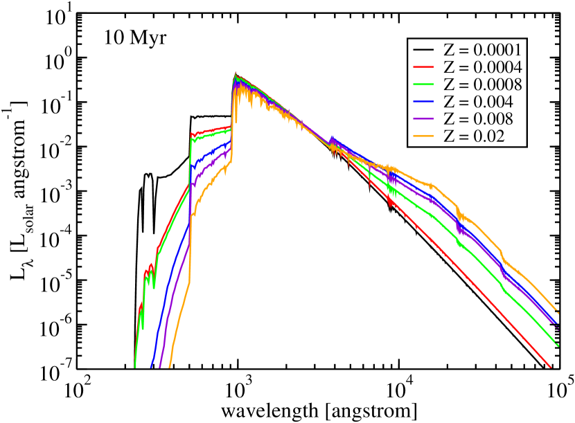
Figure 1.— SSPS for $t=10$ Myr for different metallicities. IR emission increases and UV emission decreases for increasing metallicity ($Z$).

The PEGASE.2 code does not produce accurate SSPS for high mass Population III (low $Z$) stars. Therefore, for SSPS at $Z=0$, we follow Gilmore (2012) and use the results from Schaerer (2002) for high mass stars. For $Z=0$ stars with $m<5$, we use the PEGASE.2 results; for $m>5$, we assume the stars are blackbodies with temperatures and luminosities given by Table 3 of Schaerer (2002) for lifetimes given by Table 4 of Schaerer (2002).

Once SSPS are produced for a grid of stellar population ages and metallicities, we interpolate to find the SSPS $L_{\lambda}(t,Z)$ for any $t$ and $Z$.

2.6. Dust Extinction

A fraction $f_{\ esc,d}(\lambda,z)$ of photons will escape absorption by dust. Driver et al. (2008) calculated the average of this fraction at $z\approx 0$ from fitting a dust model to 10,000 nearby galaxies. The resulting fraction at $z\approx 0$ fit by Razzaque et al. (2009), resulting in

$$f_{\rm esc,d}(\lambda,z=0)=\left\{\begin{array}[]{ll}0.688+0.556\log_{10}\lambda;&\lambda\leq 0.167\\ 0.151-0.136\log_{10}\lambda;&0.167<\lambda\leq 0.218\\ 1.000+1.148\log_{10}\lambda;&0.22<\lambda\leq 0.422\\ 0.728+0.422\log_{10}\lambda;&0.422<\lambda\end{array}\right.\ ,$$ (14)

where $\lambda$ is wavelength in $\mu$m. The dust extinction evolves with redshift; Abdollahi et al. (2018) fit a collection of measurements with a curve as a function of $z$. We assume the normalization of $f_{\rm fesc,d}(\lambda,z)$ evolves with $z$ following this curve, so that

$$f_{\rm esc,d}(\lambda,z)=\frac{f_{\rm esc,d}(\lambda,z=0)}{f_{\rm esc,d}(\lambda=0.15\ \mu\mathrm{m},z=0)}\times 10^{-0.4A(z)}$$ (15)

where

$$A(z)=m_{d}\frac{(1+z)^{n_{d}}}{1+[(1+z)/p_{d}]^{q_{d}}}\ ,$$ (16)

with the Abdollahi et al. (2018) fit results $m_{d}=1.49$, $n_{d}=0.64$, $p_{d}=3.4$, $q_{d}=3.54$. A similar fit was done by Puchwein et al. (2019) using a slightly different functional form.

We also use a dust model where

$$f_{\rm esc,d}(\lambda,z=0)=\left\{\begin{array}[]{ll}f_{\rm esc,2}+(f_{\rm esc,2}-f_{\rm esc,1})/(\log_{10}\lambda_{2}-\log_{10}\lambda_{1})\log_{10}\lambda;&\lambda\leq\lambda_{2}\\ f_{\rm esc,3}+(f_{\rm esc,3}-f_{\rm esc,2})/(\log_{10}\lambda_{3}-\log_{10}\lambda_{2})\log_{10}\lambda;&\lambda_{2}<\lambda\leq\lambda_{3}\\ f_{\rm esc,4}+(f_{\rm esc,4}-f_{\rm esc,3})/(\log_{10}\lambda_{4}-\log_{10}\lambda_{3})\log_{10}\lambda;&\lambda_{3}<\lambda\leq\lambda_{4}\\ f_{\rm esc,5}+(f_{\rm esc,5}-f_{\rm esc,4})/(\log_{10}\lambda_{5}-\log_{10}\lambda_{4})\log_{10}\lambda;&\lambda_{4}<\lambda\\ \end{array}\right.$$ (21)

where $\lambda_{1}=0.15\ \mu$m, $\lambda_{2}=0.167\ \mu$m, $\lambda_{3}=0.218\ \mu$m, $\lambda_{4}=0.422\ \mu$m, $\lambda_{5}=2.0\ \mu$m. Here $\{f_{\rm esc,k},k=1..5\}$ are free parameters.

2.7. Star Formation

We use two parameterizations for the comoving SFRD as a function of redshift. We primarily use the formulation from Madau & Dickinson (2014),

$$\psi_{\rm MD}(z)=a_{s}\frac{(1+z)^{b_{s}}}{1+[(1+z)/c_{s}]^{d_{s}}}$$ (22)

where $a_{s}$, $b_{s}$, $c_{s}$, and $d_{s}$ are free parameters. We also use a version similar to the piecewise function from Hopkins & Beacom (2006),

$$\psi_{\rm piece}(z) =10^{a_{s}}\left\{\begin{array}[]{ll}\zeta^{b_{s}}&z<z_{1}\\ \zeta_{1}^{b_{s}-c_{s}}\zeta^{c_{s}}&z_{1}\leq z<z_{2}\\ \zeta_{1}^{b_{s}-c_{s}}\zeta_{2}^{c_{s}-d_{s}}\zeta^{d_{s}}&z_{2}\leq z<z_{3}\\ \zeta_{1}^{b_{s}-c_{s}}\zeta_{2}^{c_{s}-d_{s}}\zeta_{3}^{d_{s}-e_{s}}\zeta^{e_{s}}&z_{3}\leq z<z_{4}\\ \zeta_{1}^{b_{s}-c_{s}}\zeta_{2}^{c_{s}-d_{s}}\zeta_{3}^{d_{s}-e_{s}}\zeta_{4}^{e_{s}-f_{s}}\zeta^{f_{s}}&z_{3}\leq z\\ \end{array}\right.$$ (28)

where $a_{s}$, $b_{s}$, $c_{s}$, $d_{s}$, $e_{s}$, and $f_{s}$ are free parameters, and we use the notation $\zeta=(1+z)$ and $\{\zeta_{k}=(1+z_{k}),k=1..4\}$. We fix $z_{1}=1.0$, $z_{2}=2.0$, $z_{3}=3.0$, $z_{4}=4.0$.

2.8. Luminosity Density

The comoving stellar luminosity density (i.e., luminosity per unit comoving volume) is given as a function of comoving dimensionless energy $\epsilon=hc/(\lambda m_{e}c^{2})$ by

$$\epsilon j^{\rm stars}(\epsilon;z) =m_{e}c^{2}\epsilon^{2}\frac{dN}{dtd\epsilon dV}$$

$$=f_{\rm esc,H}(\epsilon)f_{\rm esc,d}(\lambda,z)\$$

$$\times\int_{z}^{z_{\max}}dz_{1}\ L_{\star}(t_{\star}(z,z_{1}),Z(z_{1}))\ \psi(z_{1})\left|\frac{dt}{dz_{1}}\right|\ ,$$ (29)

where $L_{\star}(t,Z)=\lambda\times L_{\lambda}(t,Z)$. We assume all photons at energies greater than 13.6 eV are absorbed by H I gas, so that

$$f_{\rm esc,H}(\epsilon)=\left\{\begin{array}[]{ll}1&m_{e}c^{2}\epsilon<13.6\ \mathrm{eV}\\ 0&m_{e}c^{2}\epsilon\geq 13.6\ \mathrm{eV}\end{array}\right.\ .$$ (30)

The age of the stellar population $t_{\star}(z,z_{1})$ can be found by computing the integral

$$t_{\star}(z,z_{1})=\int_{z}^{z_{1}}dz^{\prime}\ \left|\frac{dt}{dz^{\prime}}\right|\ ,$$ (31)

which has an analytic solution (Razzaque et al., 2009).

We assume that the total energy absorbed by dust is re-emitted in the infrared in three blackbody dust components. These three components are a large grain component with temperature $T_{1}$ (left as a free parameter), a small grain component with temperature $T_{2}=70$ K, and a component representing polycyclic aromatic hydrocarbons as a blackbody with temperature $T_{3}=450$ K. The comoving dust luminosity density is then

$$\epsilon j^{\rm dust}(\epsilon;z) =\frac{15}{\pi^{4}}\int d\epsilon\left[\frac{1}{f_{\rm esc,d}(\lambda,z)}-1\right]j^{\rm stars}(\epsilon;z)$$

$$\times\sum_{n=1}^{3}\frac{f_{n}}{\Theta_{n}^{4}}\frac{\epsilon^{4}}{\exp[\epsilon/\Theta_{n}]-1}$$ (32)

where $\Theta_{n}=k_{B}T_{n}/(m_{e}c^{2})$ is the dimensionless temperature of a particular component and $f_{n}<1$ is the fraction of the emission absorbed by dust that is reradiated in a particular dust component. We use $f_{1}$ and $f_{2}$ as free parameters, with $f_{3}$ constrained by $f_{1}+f_{2}+f_{3}=1$. The temperatures of each component are fixed to the values given above.

Once the stellar and dust luminosity densities are calculated, the total luminosity density is simply

$$\epsilon j^{\rm tot}(\epsilon;z)=\epsilon j^{\rm stars}(\epsilon;z)+\epsilon j^{\rm dust}(\epsilon;z)\ .$$ (33)

2.9. EBL

The proper frame energy density as a function of the proper frame dimensionless energy $\epsilon_{p}$ is

$$\epsilon_{p}u_{\rm EBL,p}(\epsilon_{p};z)=(1+z)^{4}\int_{z}^{z_{\max}}dz_{1}\frac{\epsilon^{\prime}j^{\rm tot}(\epsilon^{\prime};z_{1})}{(1+z_{1})}\left|\frac{dt}{dz}\right|\ ,$$ (34)

where

$$\epsilon^{\prime}=\frac{1+z_{1}}{1+z}\epsilon_{p}\ .$$ (35)

EBL intensity is usually measured in units nW m^-2 sr^-1; the energy density can be converted to intensity via

$$\epsilon_{p}I_{\rm EBL}(\epsilon_{p};z)=\frac{c}{4\pi}\epsilon_{p}u_{\rm EBL,p}(\epsilon_{p};z)\ .$$ (36)

2.10. Gamma-ray Absorption

The absorption optical depth

$$\tau_{\gamma\gamma}(\epsilon_{1},z) =\frac{c\pi r_{e}^{2}}{\epsilon_{1}^{2}m_{e}c^{2}}\ \int^{z}_{0}\frac{dz^{\prime}}{(1+z^{\prime})^{2}}\ \left|\frac{dt_{*}}{dz^{\prime}}\right|\$$

$$\times\int^{\infty}_{\frac{1}{\epsilon_{1}(1+z^{\prime})}}d\epsilon_{p}\frac{\epsilon_{p}u_{EBL,p}(\epsilon_{p};z^{\prime})}{\epsilon_{p}^{4}}\ \bar{\phi}(\epsilon_{p}\epsilon_{1}(1+z^{\prime}))\ ,$$ (37)

where

$$\bar{\phi}(s_{0})=\frac{1+\beta_{0}^{2}}{1-\beta_{0}^{2}}\ln w_{0}-\beta_{0}^{2}\ln w_{0}-\frac{4\beta_{0}}{1-\beta_{0}^{2}}$$ (38)

$$+2\beta_{0}+4\ln w_{0}\ln(1+w_{0})-4L(w_{0})\ ,$$

$\beta_{0}^{2}=1-1/s_{0}$, $w_{0}=(1+\beta_{0})/(1-\beta_{0})$, and

$$L(w_{0})=\int^{w_{0}}_{1}dw\ w^{-1}\ln(1+w)\$$ (39)

(Gould & Schréder, 1967b; Brown et al., 1973).

3. Data

We fit a variety of data with our model using an MCMC algorithm. The data include $\gamma$-ray absorption data from blazars, and luminosity density, stellar mass density, EBL intensity, and dust extinction data from galaxy surveys. We briefly describe these data in Sections 3.1, 3.2, 3.3, 3.4, and 3.5, respectively, and the MCMC technique in Section 3.6.

3.1. Gamma-ray Absorption Data

Ackermann et al. (2012) developed a method to determine the EBL absorption optical depth from $\gamma$-ray observations of a large sample of blazars. This involved a joint likelihood fit to a large statistical sample of blazars, using the LAT spectrum in the $1.0$—$10\ \mathrm{GeV}$ (where the $\gamma$-ray absorption should be negligible) extrapolated to $>10\ \mathrm{GeV}$ as the intrinsic spectrum of each source, and allowing the normalization of the absorption optical depth to be an additional free parameter for all sources within a redshift and energy bin. They applied their method to 150 blazars in 3 redshift bins, using $\approx 4$ years of data. Abdollahi et al. (2018) applied this technique to a much larger sample and much more data: 9 years of LAT data from 739 blazars, now divided into 12 redshift bins. They also included a constraint from the LAT detection of GRB 080916C (see also Desai et al., 2017). Desai et al. (2019) applied this method to measure the absorption optical depth using 106 IACT VHE $\gamma$-ray spectra from 38 blazars from the sample compiled by Biteau & Williams (2015). They divided their sample into two redshift bins. We include in our fit here the absorption optical depth measured with the 739 blazars and 1 GRB measured by Abdollahi et al. (2018), and measured with the 106 VHE spectra by Desai et al. (2019). The reported errors for all of the $\gamma$-ray absorption data include both statistical and systematic uncertainties.

Generally, $\gamma$-ray telescopes are only able to measure values of the EBL absorption optical depth in the range $10^{-2}\lesssim\tau_{\gamma\gamma}\lesssim 5$. This is because, for low values of $\tau_{\gamma\gamma}$, e.g., $\exp(-0.01)\approx 0.99$, absorption will be negligible, and there will be nothing to measure. At high values of $\tau_{\gamma\gamma}$, e.g., $\exp(-5)\approx 0.007$, almost all of the $\gamma$-rays will be absorbed, and there will be no $\gamma$-ray signal to measure. Outside of this range, however, it is possible to put upper limits on $\tau_{\gamma\gamma}$ at lower optical depths, and lower limits on $\tau_{\gamma\gamma}$ at higher optical depths.

One should also note that Lorentz invariance violation could modify the $\gamma\gamma$ pair production threshold, reducing the absorption optical depth to $\gamma$-rays at $\gtrsim 10\ \mathrm{TeV}$ (e.g., Kifune, 1999). In this cases, $\gamma$-rays at these energies could be potentially detectable with the upcoming Cherenkov Telescope Array (Abdalla & Böttcher, 2018; Abdalla et al., 2021). If axion-like particles exist, $\gamma$-ray photons could convert to them and in principle avoid $\gamma\gamma$ pair production (de Angelis et al., 2007; Sánchez-Conde et al., 2009). However, there is no evidence that this is occuring (Buehler et al., 2020).

3.2. Luminosity Density Data

We have searched through the literature to compile a large amount of luminosity density measurements from galaxy surveys to fit with our EBL model. We particularly found useful the compilations by Helgason & Kashlinsky (2012); Stecker et al. (2012); Scully et al. (2014); Madau & Dickinson (2014); and Stecker et al. (2016). Our luminosity data compiled from the literature can be found in Table 2. The redshift and wavelength coverage can be seen in Figure 2. The majority of the data comes from three sources: Tresse et al. (2007); Andrews et al. (2017); and Saldana-Lopez et al. (2021). Coverage is fairly complete at $z\lesssim 1$, mainly due to the work of Andrews et al. (2017) using data from the Galaxy and Mass Assembly (GAMA) and Cosmic Origins Survey (COSMOS) projects. They included data from a wide variety of instruments across the electromagnetic spectrum. There is less complete coverage at longer wavelengths moving to higher $z$. Saldana-Lopez et al. (2021) made use of the CANDELS programs to get fairly complete wavelength coverage of the luminosity density up to $z=6$. At $z\gtrsim 6$, only UV luminosity density data is available. These high-$z$ UV data are due to deep exposures with the WFC3 instrument on the Hubble Space Telescope (HST) (Finkelstein et al., 2015; McLeod et al., 2016; Bouwens et al., 2016). However, see Oesch et al. (2018). Much of the luminosity density data we use here was published after our last model (Finke et al., 2010), giving the work here a different view of the luminosity density, particularly at high redshift. Occasionally we needed to convert luminosity density from $L_{\odot}\ \mathrm{Mpc}^{-3}$ to $\mathrm{W}\ \mathrm{Mpc}^{-3}$, which we did using $L_{\odot}=3.826\times 10^{26}\ \mathrm{W}$.

When necessary we converted the luminosity density measurements to a cosmology with $H_{0}=70\ \mathrm{km}\ \mathrm{s}^{-1}\ \mathrm{Mpc}^{-1}$ and $\Omega_{m}=0.30$ assumed in most of our models (Section 2.1). In several of our model fits (Models A.c and D.c), we allow these cosmological parameters to be free parameters. In these cases, the model luminosity density is converted from the model cosmology to the “standard” $(H_{0},\Omega_{m})=(70\ \mathrm{km}\ \mathrm{s}^{-1}\ \mathrm{Mpc}^{-1},0.30)$ cosmology used in the measurements with

$$j(\epsilon,z)_{\rm std}=j(\epsilon,z)_{\rm model}\times\frac{\left|dt/dz\right|_{\rm model}}{\left|dt/dz\right|_{\rm std}}\ .$$ (40)

Table 2Luminosity density data used in fits.

$z$	$\lambda\ [\mu\mathrm{m}]$	$\epsilon j(\epsilon;z)\ [\mathrm{W}\ \mathrm{Mpc}^{-3}]$	Reference
0.0	0.1535	$0.84^{+0.07}_{-0.07}\times 10^{34}$	a
0.0	0.2301	$0.84^{+0.07}_{-0.07}\times 10^{34}$	a
0.0	0.3557	$1.47^{+0.07}_{-0.07}\times 10^{34}$	a
0.0	0.4702	$3.29^{+0.07}_{-0.07}\times 10^{34}$	a
0.0	0.6175	$4.41^{+0.14}_{-0.14}\times 10^{34}$	a
0.0	0.7491	$4.62^{+0.14}_{-0.14}\times 10^{34}$	a
0.0	0.8946	$4.69^{+0.14}_{-0.14}\times 10^{34}$	a
0.0	1.0305	$4.20^{+0.21}_{-0.21}\times 10^{34}$	a
0.0	1.2354	$3.78^{+0.21}_{-0.21}\times 10^{34}$	a
0.0	1.6458	$3.78^{+0.21}_{-0.21}\times 10^{34}$	a

Note. — ^aDriver et al. (2012). ^bAndrews et al. (2017). ^cTresse et al. (2007). ^dArnouts et al. (2007). ^eBeare et al. (2019). ^fBudavári et al. (2005). ^gCucciati et al. (2012). ^hDahlen et al. (2007). ⁱMarchesini et al. (2012). ^jSchiminovich et al. (2005). ^kStefanon & Marchesini (2013). ^lBouwens et al. (2016). ^mFinkelstein et al. (2015). ⁿMcLeod et al. (2016). ^oDai et al. (2009). ^pBabbedge et al. (2006). ^qTakeuchi et al. (2006). ^rSaldana-Lopez et al. (2021). ^sYoshida et al. (2006).

This table is published in its entirety in the machine-readable format. A portion is shown here for guidance regarding its form and content.

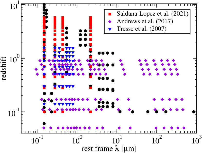
Figure 2.— A plot indicating the rest-frame wavelength and redshift of the luminsity density data from the literature that we use. Data from Tresse et al. (2007); Andrews et al. (2017); and Saldana-Lopez et al. (2021) are represented by symbols as shown in the legend; all other sources are represented by circles.

3.3. Stellar Mass Density Data

Madau & Dickinson (2014) have compiled a large number of cosmological stellar mass density measurements. Stellar mass density measurements are model-dependent, particularly on the IMF. Madau & Dickinson (2014) have scaled their mass density calculation to a Salpeter IMF.

We use stellar mass density data from the compilation by Madau & Dickinson (2014). For models that use the BG03 IMF, we adjusted the stellar mass density as follows:

$$\rho_{\rm BG03}=\rho_{\rm Sal}\times\frac{1-R_{\rm BG03}}{1-R_{\rm Sal}}$$ (41)

where $\rho_{\rm BG03}$ and $\rho_{\rm Sal}$ are the mass density data with the BG03 and Salpeter IMFs, respectively, and $R_{\rm BG03}$ and $R_{\rm Sal}$ are the return fractions (Equation 6) for the BG03 and Salpeter IMFs, respectively. We use $R_{\rm BG03}=0.49$ and $R_{\rm Sal}=0.3$ for all $z$ and $\bar{Z}$, although the actual values are metallicity-dependent, these are roughly the midpoint of the different values (Table 1). To take into account the errors from assuming all stars have the same $R$, we increased the error on all $\rho_{\rm BG03}$ by 10%, added in quadrature; that is, the resulting error in $\rho_{\rm BG03}$ is

$$\sigma_{\rm BG03}=\sqrt{\sigma_{\rm Sal}^{2}+(0.1\rho_{\rm BG03})^{2}}$$ (42)

where $\sigma_{\rm Sal}$ is the error on $\rho_{\rm Sal}$ reported by Madau & Dickinson (2014).

Similar to the luminosity density, when the cosmological parameters are allowed to vary in the model, we convert the model stellar mass density to the standard cosmology used in the stellar mass density measurements with

$$\rho(z)_{\rm std}=\rho(z)_{\rm model}\times\frac{\left|dt/dz\right|_{\rm model}}{\left|dt/dz\right|_{\rm std}}\ .$$ (43)

3.4. EBL intensity constraints at z=0

We include in our model fit the $z=0$ EBL intensity integrated galaxy light lower limits from Driver et al. (2016). This integrated galaxy light represents the resolved component of the EBL. The lower limits span a wavelength range $0.15\ \mu\mathrm{m}<\lambda<500\ \mu\mathrm{m}$ and were derived from galaxy number count data from a variety of ground- and space-based sources.

3.5. UV Dust Extinction Data

We use the far ultraviolet (FUV; $0.15\ \mu\mathrm{m}$) dust extinction as measured by Burgarella et al. (2013) and Andrews et al. (2017). Burgarella et al. (2013) derive the extinction from the ratio of the FUV to integrated infrared luminosity functions. Andrews et al. (2017) determined these FUV extinction values by fitting a dust model to a variety of multiwavelength data.

3.6. MCMC fit

We use the open-source python-implemented MCMC code emcee (Foreman-Mackey et al., 2013) to determine our best fit model parameters and their posterior probabilities. This code implements the affine-invariant ensemble sampler of Goodman & Weare (2010). It generates several MCMC chains (“walkers”) that evolve through the model space simultaneously, with different model parameters (represented by $\overrightarrow{\theta}$ below) each time step. We typically use 86 walkers here. We do not use the first $\approx 2000$ states for each walker (slightly different for each model) to avoid the “burn-in” period.

The MCMC algorithm uses a likelihood function, $\mathcal{L}\propto\exp(-\chi^{2})$. For most of our models, we include fits to the $\gamma$-ray opacity ($\tau$), luminosity density ($j$), stellar mass density ($\rho$), EBL intensity ($I_{\rm EBL}$), and FUV dust extinction ($A_{\rm FUV}$) data described above. Thus,

$$\chi^{2} =\sum_{i}\frac{[\tau_{\rm obs}(E_{i},z_{i})-\tau_{\rm model}(\overrightarrow{\theta}|E_{i},z_{i})]^{2}}{\sigma_{\tau,i}^{2}}+\sum_{i}\frac{[j_{\rm obs}(\lambda_{i},z_{i})-j_{\rm model}(\overrightarrow{\theta}|\lambda_{i},z_{i})]^{2}}{\sigma_{j,i}^{2}}$$

$$+\sum_{i}\frac{[\rho_{\rm obs}(z_{i})-\rho_{\rm model}(\overrightarrow{\theta}|z_{i})]^{2}}{\sigma_{\rho,i}^{2}}+\sum_{i}\frac{[I_{\rm EBL,obs}(\lambda_{i},z_{i})-I_{\rm EBL,model}(\overrightarrow{\theta}|\lambda_{i},z_{i})]^{2}}{\sigma_{I_{\rm EBL},i}^{2}}$$

$$+\sum_{i}\frac{[A_{\rm FUV,obs}(z_{i})-A_{\rm FUV,model}(\overrightarrow{\theta}|z_{i})]^{2}}{\sigma_{A_{\rm FUV},i}^{2}}\ .$$ (44)

In some cases the upper and lower errors differ. In these cases, if $\tau_{\rm obs}(E_{i},z_{i})>\tau_{\rm model}(\overrightarrow{\theta}|E_{i},z_{i})$ we use the lower error for $\sigma_{\tau,i}$; otherwise we use the upper error. We similarly discriminate between upper and lower errors for the other data points.

We use flat priors for all our parameters with appropriately large limits. Our results are generally independent of the limits on the priors except for the fit to the $\tau_{\gamma\gamma}$ only (Model B) as described by Abdollahi et al. (2018).

4. Results

The median and 68% confidence intervals of the posterior probabilities of the model parameters resulting from all of our MCMC fits are reported in Table 3. The table also summarizes the differences in the models, including the IMF and SFR parameterization used, the data sets used, and the parameters that were fixed or free during the model fits.

Table 3Model parameters.

	Model A	Model A.c	Model B	Model C	Model D	Model D.c	Model E
IMF	BG03	BG03	BG03	BG03	Sal	Sal	BG03
SFR	MD14	MD04	MD14	MD14	MD14	MD14	piece
dust	free	free	fixed	free	free	free	free
cosmology	fixed	free	fixed	fixed	fixed	free	fixed
data	all	all	$\tau_{\gamma\gamma}$	$j+\rho$	all	all	all
$a_{s}\ [10^{-3}]$	$9.2^{+0.5}_{-0.4}$	$9.1^{+0.5}_{-0.6}$	$9.6^{+7.3}_{-5.2}$	$9.4\pm 0.4$	$13.3\pm 0.6$	$14.5^{+1.2}_{-0.8}\pm 0.7$	$-2.04\pm 0.02$
$b_{s}$	$2.79^{+0.10}_{-0.09}$	$2.63\pm 0.14$	$3.1^{1.4}_{-1.0}$	$2.73^{+0.11}_{-0.10}$	$2.61^{+0.10}_{-0.09}$	$2.71\pm 0.12$	$2.81\pm 0.11$
$c_{s}$	$3.10^{+0.10}_{-0.09}$	$3.22^{+0.10}_{-0.12}$	$3.0^{+0.7}_{-0.5}$	$3.11^{+0.11}_{-0.09}$	$2.91\pm 0.08$	$2.95^{+0.11}_{-0.09}$	$1.25\pm 0.25$
$d_{s}$	$6.97^{+0.16}_{-0.15}$	$6.89^{+0.22}_{-0.16}$	$8.0^{+1.4}_{-1.5}$	$6.91\pm 0.18$	$6.03\pm 0.09$	$6.26^{+0.19}_{-0.22}$	$-1.25^{+0.60}_{-0.57}$
$e_{s}$	N/A	N/A	N/A	N/A	N/A	N/A	$-1.84^{+0.74}_{-0.70}$
$f_{s}$	N/A	N/A	N/A	N/A	N/A	N/A	$-4.40^{+0.19}_{-0.23}$
$f_{esc,1}$	$1.88^{+0.24}_{-0.44}$	$1.83^{+0.42}_{-0.53}$	$0.257$	$1.96^{+0.23}_{-0.39}$	$1.94^{+0.25}_{-0.44}$	$0.68^{+0.52}_{-0.37}$	$1.93^{+0.22}_{-0.42}$
$f_{esc,2}$	$2.18^{+0.29}_{-0.51}$	$2.08^{+0.54}_{-0.57}$	$0.287$	$2.58^{+0.36}_{-0.51}$	$2.19^{0.30}_{-0.49}$	$0.77^{+0.64}_{-0.42}$	$2.26^{+0.26}_{-0.49}$
$f_{esc,3}$	$2.93^{+0.38}_{-0.70}$	$2.73^{+0.51}_{-0.82}$	$0.271$	$2.85^{+0.36}_{-0.58}$	$2.99^{+0.40}_{-0.70}$	$1.01^{+0.79}_{-0.52}$	$3.00^{+0.37}_{-0.65}$
$f_{esc,4}$	$3.93^{+0.49}_{-0.93}$	$3.68^{+0.77}_{-1.12}$	$0.628$	$4.00^{+0.42}_{-0.82}$	$3.62^{+0.47}_{-0.81}$	$1.20^{+0.87}_{-0.61}$	$4.01^{+0.43}_{-0.87}$
$f_{esc,5}$	$8.57^{+1.07}_{-2.00}$	$8.16^{+1.51}_{-2.68}$	$0.959$	$8.73^{+0.92}_{-1.76}$	$8.50^{+1.07}_{-1.93}$	$2.91^{+2.21}_{-1.55}$	$8.80^{+0.88}_{-1.89}$
$m_{d}$	$1.52^{+0.04}_{-0.04}$	$1.43^{+0.04}_{-0.03}$	$1.49$	$1.59\pm 0.05$	$1.51\pm 0.04$	$1.47^{+0.05}_{-0.04}$	$1.53\pm 0.04$
$n_{d}$	$0.35^{+0.04}_{-0.04}$	$0.41^{+0.05}_{-0.04}$	$0.644$	$0.35\pm 0.04$	$0.17\pm 0.03$	$0.22\pm 0.05$	$0.37^{+0.06}_{-0.05}$
$p_{d}$	$4.12^{+0.13}_{-0.13}$	$4.14^{+0.15}_{-0.16}$	$3.4$	$4.15^{+0.12}_{-0.13}$	$3.86^{+0.13}_{-0.12}$	$3.91^{+0.13}_{-0.18}$	$4.71^{+0.32}_{-0.39}$
$q_{d}$	$5.89^{+0.55}_{-0.48}$	$5.12^{+0.36}_{-0.57}$	$3.54$	$6.11^{+0.54}_{-0.48}$	$6.95^{+0.75}_{-0.66}$	$5.97^{+0.66}_{-0.57}$	$3.67^{+0.70}_{-0.57}$
$f_{1}$	$0.56^{+0.17}_{-0.18}$	$0.13^{+0.20}_{-0.06}$	$0.48^{+0.24}_{-0.30}$	$0.60^{+0.14}_{-0.18}$	$0.55^{+0.16}_{-0.17}$	$0.19\pm 0.11$	$0.59^{+0.15}_{-0.19}$
$f_{2}$	$0.26^{+0.18}_{-0.17}$	$0.68^{+0.06}_{-0.21}$	$0.47^{+0.32}_{-0.26}$	$0.22^{+0.18}_{-0.14}$	$0.25^{+0.17}_{-0.16}$	$0.63^{+0.10}_{-0.12}$	$0.23^{+0.20}_{-0.15}$
$T_{1}$ [K]	$60.5^{+2.3}_{-3.5}$	$40.5^{+11.7}_{-4.2}$	$40$	$61^{+2}_{-3}$	$60.8^{+2.1}_{-3.2}$	$62.8^{+2.1}_{-3.1}$	$51.9^{+6.7}_{-10.6}$
$H_{0}\ [\mathrm{km}\ \mathrm{s}^{-1}\ \mathrm{Mpc}^{-1}]$	$70$	$69.8^{+3.6}_{-3.2}$	$70$	$70$	$70$	$79.4^{+8.1}_{-4.3}$	$70$
$\Omega_{m}$	$0.3$	$0.23^{+0.3}_{-0.4}$	$0.3$	$0.3$	$0.3$	$0.29\pm 0.04$	$0.3$

4.1. Fiducial Model Comparison with Data

We consider “Model A” to be our fiducial model. This model uses the Madau & Dickinson (2014) SFRD parameterization, Equation (22), and the Baldry & Glazebrook (2003) IMF, Equation (4), and has all of the SFRD and dust extinction and emission parameters free in the fit, but keeps the cosmological parameters fixed. It fits all of the data described in Section 3: the $\gamma$-ray opacity, luminosity density, stellar mass density, and FUV dust extinction data, as well as the EBL intensity lower limits.

The luminosity densities as a function of $z$ from our model are plotted in Figure 3, and compared with data. The model is clearly a good fit to the most recent data at these wavelengths. It is interesting to note the divergence at high $z$ with the older data and model. In the FUV band, the $0.17\ \mu\mathrm{m}$ older data from Sawicki & Thompson (2006) used in the previous model by Finke et al. (2010) is plotted. Sawicki & Thompson (2006) used deep imaging with the Keck telescope. The updated deep HST observations (Bouwens et al., 2016) have found much more light at these wavelengths. Since the model from Finke et al. (2010) was designed to reproduce these observations (among others), it is not surprising that it is lower than Model A of this work. One should note that the models from Finke et al. (2010) did not extend beyond $z=6$. At $0.28\ \mu\mathrm{m}$ and $0.44\ \mu\mathrm{m}$, the older model, current model, and all data are in reasonably good agreement.

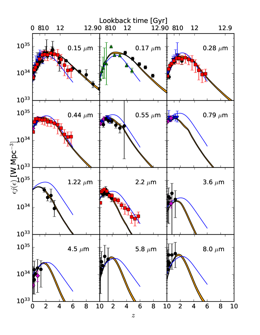
Figure 3.— The 68% contour luminosity density result for Model A as a function of $z$ at twelve wavelengths (shaded orange region). The red squares are the data from Saldana-Lopez et al. (2021), the violet dimonds represent the data from Andrews et al. (2017), and the blue downward-pointing triangles represent the data from Tresse et al. (2007). The rest of the data from galaxy surveys are plotted as the black circles. All of these data were used in the model fit, while the green upward-pointing triangles represent older, superseded data from Sawicki & Thompson (2006) that were not used in the fit. The blue curves are the luminosity densities from the older Model C from Finke et al. (2010). The wavelengths of the data and models are labeled on the plots.

As one moves to longer wavelengths, our Model A becomes lower than the older model from Finke et al. (2010), particularly at $z>2$. The model reproduces most of the data at most wavelengths shown here. For instance, the current Model A follows the data from Stefanon & Marchesini (2013) at $1.22\ \mu\mathrm{m}$, which was obviously not available to Finke et al. (2010). However, our Model A is considerably below the luminosity density measurements from Saldana-Lopez et al. (2021) at $2.2\ \mu\mathrm{m}$, particularly at $z\gtrsim 2$, despite the fact that these data were included in the fit. We think this is because of our poor modeling of the PAH component (see below). The model is generally consistent with the Saldana-Lopez et al. (2021) data at $z\lesssim 2$ where the emission is dominated by stellar emission, rather than PAH emission. The model also closely follows the lower luminosity densities of Stefanon & Marchesini (2013) at $1.2\ \mu\mathrm{m}$ and $1.6\ \mu\mathrm{m}$ at $z\lesssim 2$. The stellar models seem to be highly constraining in this wavelength range. However, this is the wavelength range identified by Conroy et al. (2009) where assumptions about all stars having the same metallicity, rather than a distribution of metallicities, can create uncertainty in emission. This is illustrated in Figure 1 where different metallicities can create significant differences at the redder wavelengths. At the longer IR wavelengths ($3.6\ \mu\mathrm{m}$ to $8.0\ \mu\mathrm{m}$), most of the data are from the work of Babbedge et al. (2006) and Dai et al. (2009), and our model fits them well. However, at these wavelengths, the data do not extend to very high redshift, and the data that do exist have large uncertainties; thus this wavelength range is not strongly constrained. This paucity of data should be rectified in the near future with the James Webb Space Telescope Mid-Infrared Instrument. At $3.6$ – $8.0\ \mu\mathrm{m}$ and $z\gtrsim 2$ our model is considerably lower than the older model from Finke et al. (2010).

The luminosity density as a function of wavelength at four redshifts is shown in Figure 4. At low redshifts ($z\leq 0.5$) the model follows the data from Andrews et al. (2017) closely. At $z=0.10$, older measurements at 3.6 – 8 $\mu\mathrm{m}$ by Babbedge et al. (2006) are generally higher but also have greater uncertaintly compared with more recent measurements by Andrews et al. (2017, see also large uncertainties in these data in Figure 3). At this redshift, our updated Model A here and the model from Finke et al. (2010) are in agreement at all wavelengths except the $\lambda\approx 3.0$ – $20\ \mu\mathrm{m}$ range, mainly due to the influence of the Babbedge et al. (2006) data on the older model. For the $\geq 12\ \mu\mathrm{m}$ measurements by Takeuchi et al. (2006), the measurements are a bit lower than the model and other measurements, but still mostly consistent with them, considering the larger uncertainties. At $z=0.5$, essentially all the data and models are in agreement.

At $z=0.9$, some separation between models and data can be seen. At this redshift, at $\lambda<1.2\ \mu\mathrm{m}$, the measurements from Tresse et al. (2007) are below the ones from Andrews et al. (2017). Our Model A follows the Tresse et al. (2007) measurements here more closely, which is quite a bit lower than Model C from Finke et al. (2010) in the $\lambda=0.8$ – $3.0\ \mu\mathrm{m}$ range. At $\lambda>30\ \mu\mathrm{m}$, the updated model is higher than the older model from Finke et al. (2010). This is due to the influence of the Andrews et al. (2017) data at these wavelengths. This redshift ($z=0.9$) is the highest redshift for which Andrews et al. (2017) have measurements.

The luminosity density at $z=3$ is a particularly interesting case. The older model from Finke et al. (2010) is quite divergent from our updated model here. In the model itself, this seems to be related to the updated stellar spectra. The data we fit is also influencial, and the updated model reproduces the data at $\lambda<3\ \mu\mathrm{m}$ well. Most of the optical-near IR measurements used at this redshift (Marchesini et al., 2012; Stefanon & Marchesini, 2013; Saldana-Lopez et al., 2021) did not exist when Finke et al. (2010) created their model. The only data point at $z=3$ that is not reproduced by the model is the $\lambda=2.2\ \mu\mathrm{m}$ measurement by Saldana-Lopez et al. (2021). This could be due to the approximation of the PAH component by a blackbody. A more realistic treatment of this component might reproduce the high redshift $2.2\ \mu\mathrm{m}$ data better, where their is considerable disagreement between data and model (see Figure 3). Another possibility is that out model is underestimating the metallicity (see Figure 8), and that a higher metallicity would lead to more intense luminosity density at this wavelength (Figure 1). Finally, it could be that AGN, neglected here, could contribute to the $2.2\ \mu\mathrm{m}$ luminosity density observed by Saldana-Lopez et al. (2021). The AGN would be required to make up 70% of the $2.2\ \mu\mathrm{m}$ luminosity density at $z=3.75$, and 90% at $z=5.75$. Estimates of the AGN contribution to the EBL indicate that it likely makes no more than 10% at any relevant wavelength (Domínguez et al., 2011; Andrews et al., 2018; Abdollahi et al., 2018; Khaire & Srianand, 2019). We therefore believe it unlikely that AGN could be the reason for the discrepancy here.

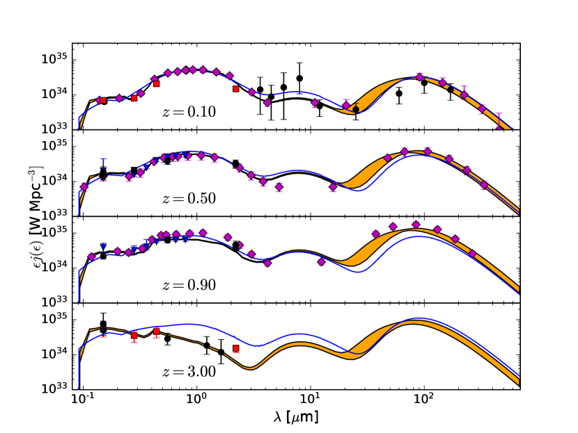
Figure 4.— The 68% contour luminosity density result for Model A as a function of $\lambda$ at four redshifts (shaded orange region). The red squares are the data from Saldana-Lopez et al. (2021), the violet dimonds represent the data from Andrews et al. (2017), and the blue downward-pointing triangles represent the data from Tresse et al. (2007). The rest of the data from galaxy surveys used in the fit are plotted as the black circles. The blue curves are the luminosity densities from the older Model C from Finke et al. (2010). The redshifts of the data and models are labeled on the plots.

The 68% confidence interval for the EBL intensity at $z=0$ for our Model A is shown in Figure 5, along with a variety of lower limits and other models from the literature. Our model result has little uncertainty at $\lambda\lesssim 10\ \mu\mathrm{m}$, while the uncertainty grows at longer wavelengths. Our updated model’s EBL intensity is lower than most other models at $\lambda\lesssim 10\ \mu\mathrm{m}$, and quite close to being in conflict with some of the lower limits from Driver et al. (2016), and below the ones from Biteau & Williams (2015). The only lower EBL model in this wavelength range is the one from Kneiske & Dole (2010), which was designed to be the lowest possible model consistent with lower limits. At longer wavelengths, uncertainty is greater. The far-IR peak at $\approx 200\ \mu\mathrm{m}$ is greater than the older model from Finke et al. (2010), considerably lower than the one from Domínguez et al. (2011), and mostly consistent with the others.

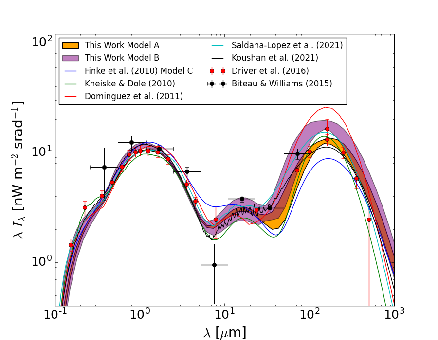
Figure 5.— The 68% contour EBL intensity results as a function of $\lambda$ at $z=0$ for Models A and B. A variety of lower limit data and models curves are shown as well, as seen in the legend.

The EBL absorption optical depth from our Model A for four redshift ranges is shown in Figure 6. These are compared with the EBL absorption measurements with the Fermi-LAT (Abdollahi et al., 2018) and IACTs (Desai et al., 2019), and the previous best fit model from Finke et al. (2010). In all cases, the 68% model errors on the absorption optical depth are quite small, typically $\lesssim 10\%$. The updated model is in quite good agreement with the data and with the previous 2010 model in almost all cases. In the lowest LAT redshift bin, $0.03<z<0.23$, the new model is $\approx 20\%$ lower than the old one at most energies. At the highest LAT redshift bin, $2.14<z<3.10$, agreement between the old and new model is good below $0.1\ \mathrm{TeV}$, although above this energy the old model predicts $\approx 50\%$ higher $\tau_{\gamma\gamma}$. Measurements of $\tau_{\gamma\gamma}$ are not found in this redshift range for energies $>0.1\ \mathrm{TeV}$, since the values of $\tau_{\gamma\gamma}$ are likely too high here to be measured (see Section 3.1).

IACTs are sensitive to higher energy $\gamma$-rays than the LAT, which makes them sensitive to $\gamma$-ray absorption at lower redshifts and higher energies. The absorption measurements with IACTs are shown in the bottom two panels of Figure 6, along with the comparison to our updated model and the Finke et al. (2010) model. Agreement between data and both the models is very good in most places. The data and the older model are $\approx 30\%$ higher in the 1 – 6 TeV range than the updated model for both redshift bins. In this energy range, the $\gamma$-rays interact with EBL photons in the range $\approx 4-24\ \mu\mathrm{m}$; see Equation (1). In this range, the EBL photons are due to the red end of the stellar photons, and the PAH component, where the old model from Finke et al. (2010) is clearly below the updated model (Figure 5).

The Model A fit is mostly constrained by the luminosity density measurements, since these are more plentiful and have smaller errors. So the discrepancy in the model and observed $\gamma$-ray absorption here could be interpreted as a discrepancy between the luminosity density and $\gamma$-ray absorption measurements.

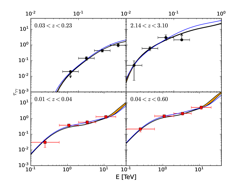
Figure 6.— The 68% contour EBL absorption optical depth as a function of observed energy for different redshift ranges for our Model A. The LAT absorption measurements from Abdollahi et al. (2018) and the IACT measurement from Desai et al. (2019) are shown as the black circles and red squares, respectively. The blue curve is the older Model C from Finke et al. (2010). Note the different energy scales on the different plots.

4.2. Physical Implications

The SFRD for the result of Model A is shown in Figure 7. The 68% SFR shows little uncertainty, rarely more than 10%. The curve from Madau & Fragos (2017) is within our model uncertainty at $z\lesssim 3$. But compared with Madau & Dickinson (2014), our model predicts a lower SFRD by a factor $\approx 2$ at $z\lesssim 3$, and by a factor $\approx 5$ at $z\gtrsim 3$. The likely discrepancy between our model and Madau & Dickinson (2014) is that the latter used a Salpeter IMF, while we used the Baldry-Glazebrook IMF. Madau & Fragos (2017) used the Kroupa IMF (Kroupa, 2001) which is more similar to the IMF we used, in that it deviates from a power-law at low masses, with fewer stars. The discrepancy at $z\lesssim 3$ is likely due to different assumptions about the evolution of metallicity and dust extinction with redshift.

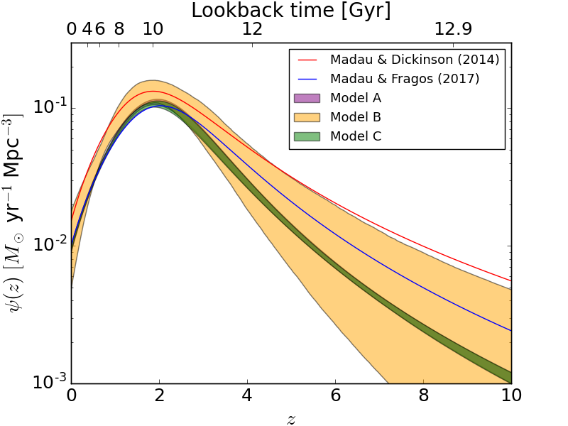
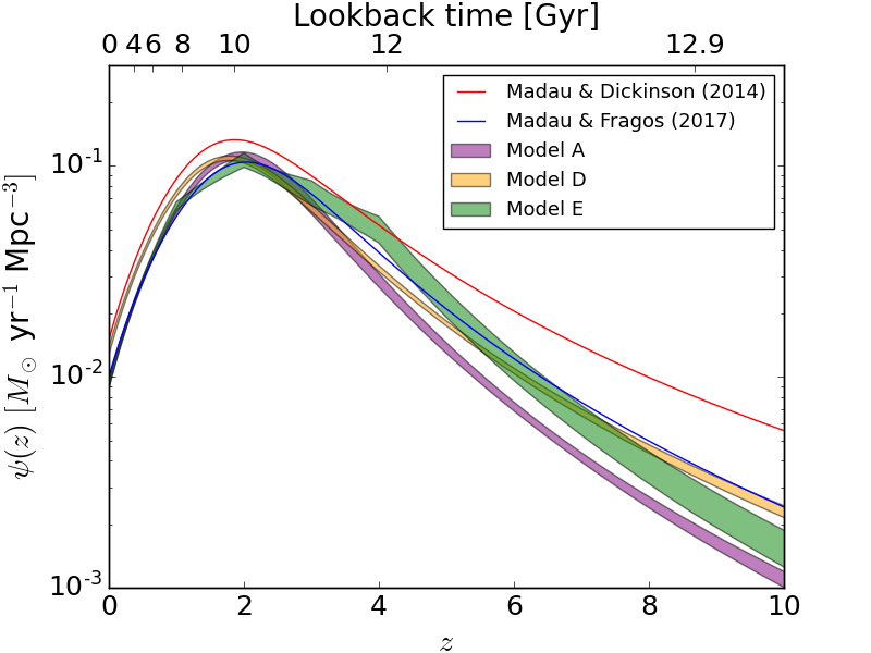
Figure 7.— The 68% contour of the SFRD, $\psi(z)$, as a function of redshift $z$ for our models, as described in the legend. Also shown are the SFRD from Madau & Dickinson (2014) and Madau & Fragos (2017). Models A and C are nearly indistinguishable on the left plot.

The resulting stellar mass density and gas-phase metallicity as a function of $z$ are shown in Figure 8. The model mass density reproduces the data quite well. Metallicity measurements from damped Ly$\alpha$ systems (Péroux & Howk, 2020, and references therein) corrected for dust depletion following De Cia et al. (2018) are also shown on the figure. Our model is clearly below these data points. We have also performed a model fit identical to Model A, but also including a fit to these points. The result is nearly identical; the metallicity data do not have enough constraining power to impact the model fit. The metallicities from Ly$\alpha$ systems compiled by Péroux & Howk (2020) (and also Biffi & Maio, 2013) have large dispersions around the mean. This can also be seen in hydrodynamic chemical evolution simulations of early galaxy star formation; these simulations indicate galaxies at $z\approx 9$ have $10^{-9}<Z<10^{-4}$ (Biffi & Maio, 2013). The model mean metallicity is compared with the mean metallicity curve from Madau & Fragos (2017). For all metallicity conversions in this figure we assumed $Z_{\odot}=0.02$. The Madau & Fragos (2017) curve was found by convolving the galaxy mass-metallicity relation for star-forming galaxies with various galaxy mass functions at different redshifts. Their results are clearly discrepant with our model, where they get much higher metallicities by $\approx 1.5-2.5$ orders of magnitude. It is not clear if these two methods are really measuring the same thing. The Madau & Fragos (2017) curve is measuring the galaxy mass-weighted mean gas phase metallicity, while the interpretation of our mean metallicity from a one-zone closed box model is not clear. The mass-metallicity relation used by Madau & Fragos (2017) has been derived from only star-forming galaxies at $z\lesssim 1.6$, so applying it to all galaxies may not be appropriate, nor using it at $z\gtrsim 1.6$. The Madau & Fragos (2017) curve is also above almost all of the damped Ly$\alpha$ data points, even when corrected for dust depletion. Madau & Fragos (2017) also note the metallicity normalization of the relation is quite uncertain. It may also be that the closed box model we use is not a good approximation for the metallicity evolution of the univese; indeed it is almost certainly an over-simplification.

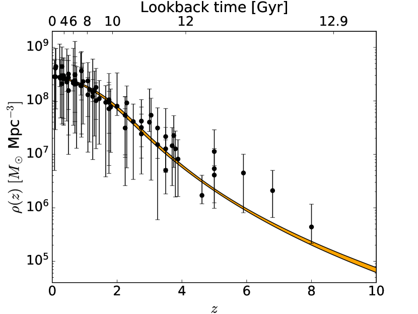
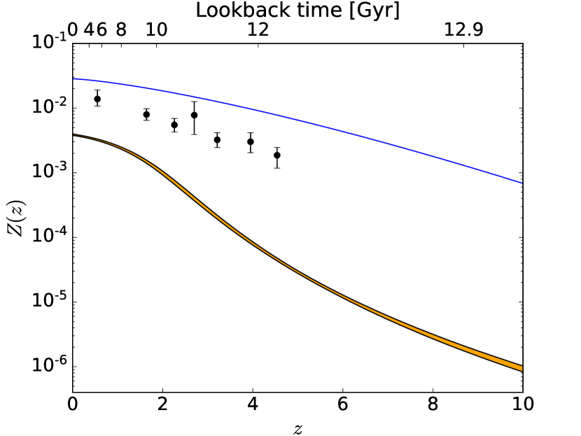
Figure 8.— left: The 68% confidence interval (orange countour) on the stellar mass density as a function of $z$ from Model A, along with data (black circles) from Madau & Dickinson (2014). right: 68% confidence interval (orange countour) on the gas-phase metallicity as a function of $z$ from Model A, along with the fit from Madau & Fragos (2017, blue curve). Mean metallicity measurements from damped Ly$\alpha$ systems corrected for dust depletion (Péroux & Howk, 2020) are shown as black circles.

The 68% contour of our Model A FUV (1500 Å) dust extinction as a function of redshift (Equation [16]) is shown in Figure 9. It clearly agrees with the data. The extinction increases with increasing redshift until about $z=2$, after which it decreases. As $z\rightarrow 10$, $A_{\rm FUV}(z)\rightarrow 0$, as expected; since dust is made of metals, and at high redshift the metallicity $Z\rightarrow 0$.

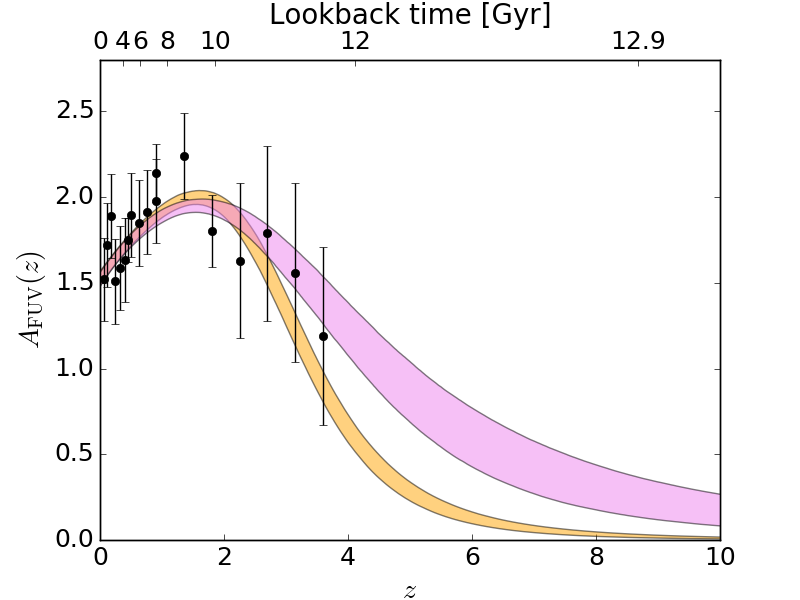
Figure 9.— The 68% contour FUV dust extinction, $A(z)$, as a function of redshift for Model A (orange shaded region) and Model E (violet shaded region). Observational data are shown as black circles.

Not only does $A(z)$, i.e. the normalization of the dust extinction curve, evolve, the shape of the curve evolves as well. The dust escape fraction, $f_{\rm esc,d}(\lambda,z)$ is shown in Figure 10 as a function of $\lambda$ for four different redshifts. The general pattern is that as the overall absorption decreases (i.e., more photons escape), it decreases at longer wavelengths much more than shorter wavelengths. At the highest redshift, $z=6$, above $\approx 0.13\ \mu\mathrm{m}$, the escape fraction goes to unity, indicating all the photons escape and none are absorbed. One can also see in this figure that the escape fraction decreases (absorption increases) until a peak at about $z=2$, and the escape fraction increases (absorption decreases) at increasing redshift at $z>2$. This is consistent with what is seen in Figure 9.

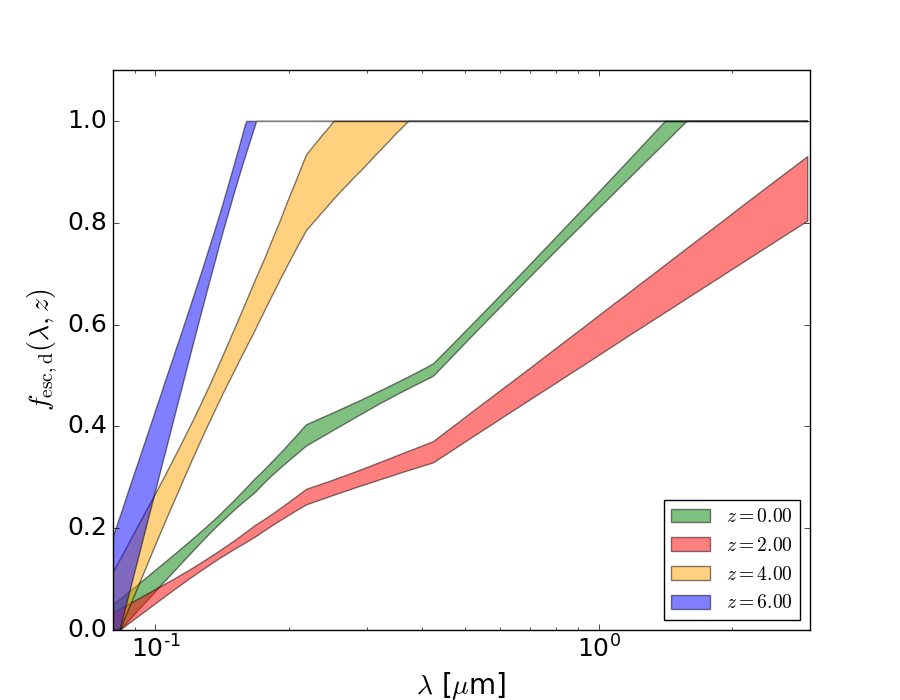
Figure 10.— The 68% contour of the dust escape fraction, $f_{d,esc}(\lambda,z)$ for Model A.

4.3. Contribution to local EBL

We can compute the contribution to the local ($z=0$) EBL intensity from sources at redshifts $<z$ for our model as (Finke et al., 2010)

$$\epsilon I(\epsilon;<z)=\frac{c}{4\pi}\int_{0}^{z}dz_{1}\frac{\epsilon^{\prime}j(\epsilon^{\prime};z_{1})}{1+z_{1}}\left|\frac{dt_{*}}{dz_{1}}\right|\ ,$$ (45)

where $\epsilon^{\prime}=\epsilon(1+z_{1})$. The result of this calculation for Model A for various wavelengths are shown Figure 11. Also shown are the resolved contributions to the build-up of the EBL, as measured by BLAST (Marsden et al., 2009) and Herschel-SPIRE (Béthermin et al., 2012). These are lower limits on the contribution to the local EBL. Based on our modeling, most of the EBL has been resolved by Herschel-SPIRE at $250\ \mu\mathrm{m}$ and $350\ \mu\mathrm{m}$, while less has been resolved at $500\ \mu\mathrm{m}$. It is also apparent that at shorter wavelengths for the stellar component of the EBL, the contribution to the local EBL is much more “local” than for the sub-mm wavelengths. Most of the local EBL comes from $z\lesssim 1$ for $\lambda<2.2\ \mu\mathrm{m}$, while for the dust component in the sub-mm, one has to go out to $z\approx 2.5$ to have all of the local EBL. This is consistent with the result of Saldana-Lopez et al. (2021).

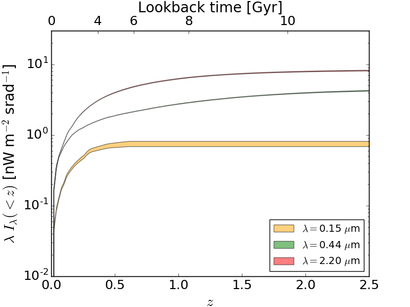
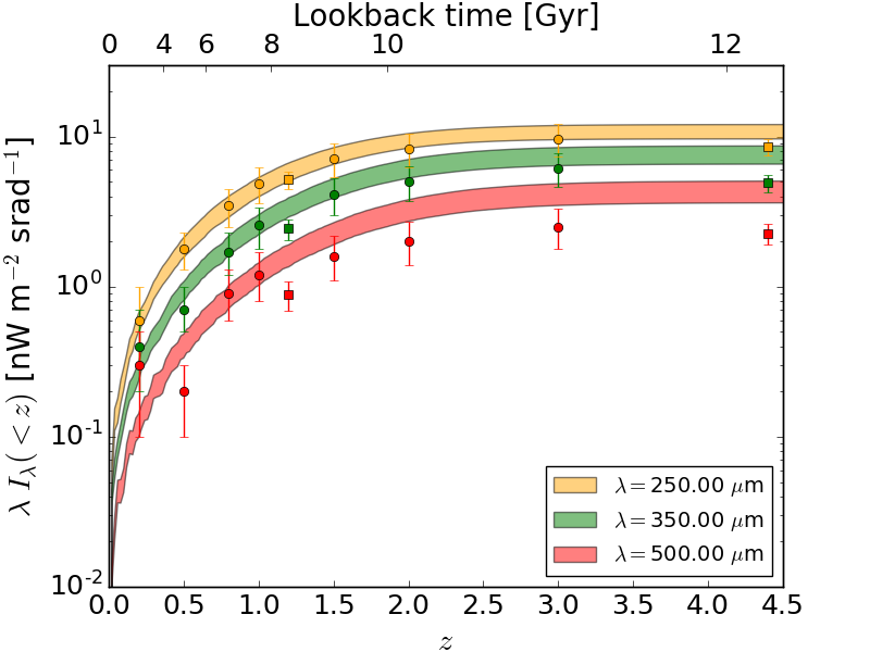
Figure 11.— The 68% contours for the contribution to the local ($z=0$) EBL that originates at redshift $<z$ for various wavelengths from Model A, as shown in the legends. The symbols represent the resolved contribution from galaxies, which are essentially lower limits on the contribution to the local EBL. Square symbols are from BLAST (Marsden et al., 2009) and circle symbols are from Herschel-SPIRE (Béthermin et al., 2012).

4.4. Results with Different Data Sets

Figure 7 also shows the resulting fit to the LAT $\gamma$-ray absorption optical depth data only (Model B). The addition of luminosity and stellar mass density data significantly increase the constraint on the SFRD. Indeed, it is not clear if the $\gamma$-ray absorption data is constraining the SFRD much more than the luminosity and stellar mass density data. To test this, we did a run similar to Model A, fitting the luminosity, stellar mass density, and dust extinction data, but without the $\gamma$-ray absorption data. This we called model C (Table 3). The results are nearly identical, as seen in Figure 7, with the Model C result having slightly larger uncertainty ($\approx 5\%$) that are nearly imperceptible in the figure. It does not seem the $\gamma$-ray absorption data is giving much more tightly constrained SFRD.

In Figure 12, we plot the luminosity density model results for the fit to the $\gamma$-ray absorption data only. It demonstrates that the $\gamma$-ray data alone can constrain the luminosity density consistent with the observed luminosity density data. Thus, although the $\gamma$-ray absorption data do not contribute strongly to the constraint due to their low $S/N$, they are valuable as an alternative, independent measurement.

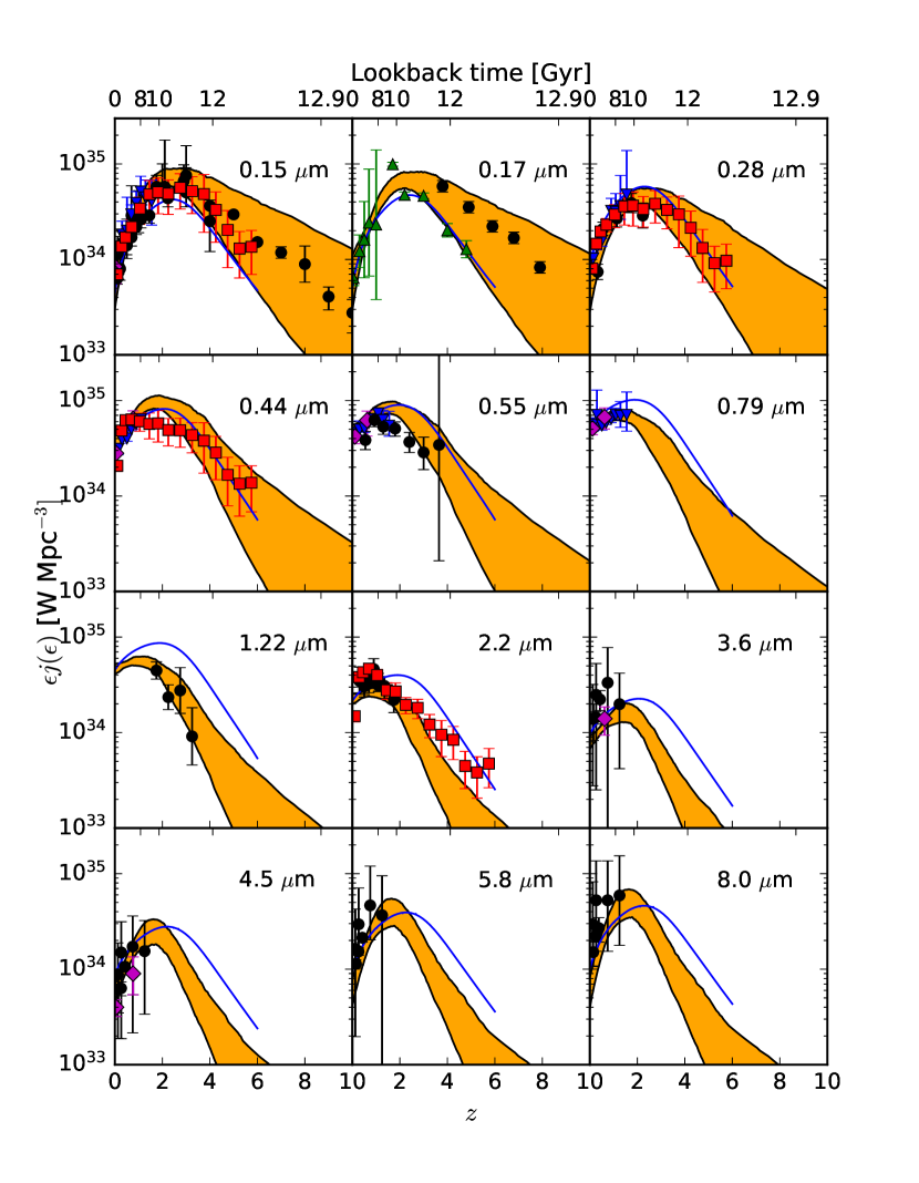
Figure 12.— The same as Figure 3 but the shaded regions are the 68% confidence intervals are for model B, the fit to $\gamma$-ray data only.

4.5. Dust Emission

The fractions of absorbed light being re-emitted by large warm grains ($f_{1}$), small hot grains ($f_{2}$), and polycyclic aromatic hydrocarbons (PAHs) are constrained by our models that include luminosity density (Table 3), although uncertainties are large. We find results that are consistent with Finke et al. (2010). For the large warm grains, we find $f_{1}=0.56^{+0.17}_{-0.18}$, compared with $f_{1}=0.6$ from the previous model; and for the small hot grains we find $f_{2}=0.26^{+0.18}_{-0.17}$, a bit higher than the old model ($f_{2}=0.05$), but within the uncertainty.

The results constrained by only the $\gamma$-rays (Model B) domonstrates that the existing $\gamma$-ray data does not strongly constrain the dust parameters, although the results of this model are completely consistent with Model A. A similar analysis was performed by de Matos Pimentel & Moura-Santos (2019), who used the VHE $\gamma$-ray spectrum of Mrk 501 from HEGRA to attempt to constrain these dust parameters as well. Our Model B results are consistent with theirs. Since the HEGRA spectrum for Mrk 501 extended to 20 TeV, they were able to a rule out a single PAH dust component; at least two dust components were required to explain the $\gamma\gamma$ absorption seen in this VHE spectrum. As de Matos Pimentel & Moura-Santos (2019) discuss, the upcoming Cherenkov Telescope Array (CTA) will reach yet higher $\gamma$-ray energies, and may be able to provide stronger constraints on the dust parameters.

The temperature we find for the warm, large grains, $T_{1}\approx 60\ \mathrm{K}$ is consistent across all models where this was a free parameter, except Model A.c. It is quiet a bit higher than the value used by Finke et al. (2010), which was $T_{1}=40\ \mathrm{K}$. Model A.c gives a value $T_{1}=40.5^{+11.7}_{-4.2}\ \mathrm{K}$, consistent with Finke et al. (2010). This model has $H_{0}$ and $\Omega_{m}$ as free parameters, and returns greater uncertainty for this parameter.

4.6. Alternative SFRD and IMF parameterizations

We wished to test our model for sensitivity to the IMF and the SFRD parameterization. The results of our model with the Salpeter IMF (Model D) can be seen in Figure 7. The results for Model D agree with Madau & Dickinson (2014) at $z\lesssim 1$, while it is increasingly below that model at higher $z$. Model D agrees reasonably well with the fiducial Model A (with a Baldry-Glazebrook IMF) at $z\lesssim 4$, but the Salpeter model gives a higher SFRD, more consistent with the one form Madau & Fragos (2017). The difference seems to be that the dust extinction is a free parameter in our model, which for Madau & Dickinson (2014) and Madau & Fragos (2017) it was not in their simpler calculation. We plan to explore different IMFs in more detail in a future publication. The EBL intensity for Model D is still quite low as with Model A, as is the absorption optical depth in the $0.03<z<0.23$ redshift bin (cf. Section 4.1).

We also want to test that the results do not depend strongly on the SFRD parameterization. In the right panel of Figure 7 we present our results with our standard MD14 SFRD parameterization and our piecewise SFRD parameterization (Equation [28]). Our results are again very similar for $z\lesssim 4$, and the piecewise SFRD model at $z\gtrsim 4$ is higher than ours. The model results do have some sensitivity to the SFRD parameterization as well. Indeed, their seems to be some degeneracy between the SFRD and dust parameters. This is demonstrated in Figure 9, where clearly the dust extinction for Models A and E differ significantly. The greater the dust extinction, the greater the SFRD must be for there to be more light to make up for that extra absorption and fit the luminosity density data. The EBL intensity and absorption optical depths for Model E are very similar to those for the fiducial Model A.

4.7. Cosmological Parameters

Since the Model A $z=0$ EBL intensity is below the lower limits from galaxy counts at many wavelengths (Figure 5) and $\gamma$-ray absorption optical depth is consistently below the observed data (Figure 6) we ran model fits with the cosmological parameters $H_{0}$ and $\Omega_{m}$ free in the fit, to see if this could resolve this discrepancy. We did model fits with both the BG03 (Model A.c) and Salpeter IMF (Model D.c). These models did not resolve the discrepancy.

Nevertheless, it is interesting to compare the results of these cosmological parameters to values determined with other methods. For Model A.c, Our value of $H_{0}=69.8^{+3.6}_{-3.2}\ \mathrm{km}\ \mathrm{s}^{-1}\ \mathrm{Mpc}^{-1}$ is consistent with measurements in the near universe from Type Ia supernovae ($73.2\pm 1.3\ \mathrm{km}\ \mathrm{s}^{-1}\ \mathrm{Mpc}^{-1}$; Riess et al., 2021b) and in the far universe from the CMB ($67.4\pm 0.5\ \mathrm{km}\ \mathrm{s}^{-1}\ \mathrm{Mpc}^{-1}$; Aghanim et al., 2020). The values of $\Omega_{m}=0.23^{+0.3}_{-0.4}$ is marginally inconsistent (between $2\sigma$ and $3\sigma$) with the values measured from Type Ia supernovae ($0.327\pm 0.016$; Riess et al., 2021b) and the CMB ($0.315\pm 0.007$; Aghanim et al., 2020). For Model D.c, the value of $H_{0}=79.4^{+8.1}_{-4.3}\ \mathrm{km}\ \mathrm{s}^{-1}\ \mathrm{Mpc}^{-1}$ is $1.4\sigma$ of from the Type Ia supernova value, and $2.8\sigma$ from the CMB value; the value of $\Omega_{m}=0.29\pm 0.04$ is consistent with both the Type Ia supernova and CMB values. It is interesting to note that for our two models with varying cosmological parameters, one is completely consistent with $H_{0}$ but slightly discrepant with $\Omega_{m}$; and vice versa for the other. The main difference between Models A.c and D.c, with different IMFs, is the number of low-mass stars produced. It seems that light produced by low-mass stars in this model has some sensitivity to cosmological parameters.

Domínguez et al. (2019) used the same EBL $\gamma$-ray absorption data we use (Section 3.1) to measure cosmological parameters, and their results were $H_{0}=67.4^{+6.0}_{-6.2}\ \mathrm{km}\ \mathrm{s}^{-1}\ \mathrm{Mpc}^{-1}$ and $\Omega_{m}=0.14^{+0.06}_{-0.07}$. Our errors are much smaller than theirs, likely due to (1) their inclusion of systematic uncertainty, which we do not include; and (2) further constraints impossed on our EBL model from stellar models and other physical constraints. Our values from Model A.c are within $1.3\sigma$ of those from Domínguez et al. (2019), while our values for Model D.c are within $2.1\sigma$ of theirs. Our values from Model A.c are clearly more consistent with this previous work, including the low value for $\Omega_{m}$.

We emphasize that the cosmological parameters $H_{0}$ and $\Omega_{m}$ from our model fits should not be considered measurments of these cosmological parameters. Unlike the work by Domínguez et al. (2019), we do not include systematic uncertainties. However, it is worth noting the cosmological parameter results depend on the chosen IMF, and light produced by low mass stars. This can inform future efforts to constrain cosmological parameters with the EBL.

5. Discussion

We have presented an update to the EBL model of Finke et al. (2010). The updated models used detailed PEGASE.2 stellar models, and track the evolution of the mean gas-phase metallicity and stellar mass density of the Universe. We have allowed the dust extinction to evolve with redshift, and used different SFRD parameterizations and IMFs. We have fit this model to a wide variety of data, including luminosity density and $\gamma$-ray absorption data. Our modeling has allowed us to measure the SFRD of the Universe with $\approx 10\%$ uncertainty for the previous $\approx 12.9$ Gyr, or $>90$% of the history of Universe (Section 4.2). The SFRD did show some dependence on the IMF and SFRD parameterization (Section 4.6). A more detailed exploration of IMFs will be presented in a future publication. We have also strongly constrained the photon escape fraction from interstellar dust in the universe and its evolution with redshift, although this also showed sensitivity to the IMF and SFRD parameterization. These discrepancies are mainly at $z\gtrsim 3$ (Figures 7 and 9). In Figure 2 one can see that at $z\gtrsim 1$, the luminosity density data becomes restricted to $\lambda\lesssim 3\ \mu\mathrm{m}$ at $z\gtrsim 1$. This likely accounts for the uncertainty at high $z$. The longer wavelength luminosity density data can nail down the dust emission, which strongly constrains the dust absorption. At high $z$ where the longer wavelength data is lacking, the dust extinction is less constrained, and hence the SFRD is as well, since there is a degeneracy between the SFRD and dust extinction. Luminosity density measurements for $\lambda\gtrsim 3\ \mu\mathrm{m}$ at $z\gtrsim 1$ could help reduce these uncertainties.

Of the data used in the fit, the luminosity density data has by far the strongest contraining power, due to the smaller uncertainty and large collection of data (see Table 2). Our fiducial model (Model A) is a reasonably good fit to almost all of the data used in the fit. Some exceptions include the $\approx 1$ – $3\ \mu\mathrm{m}$ luminosity density at $z>3$ and the EBL absorption optical depth at $z<0.6$ (Section 4.1). The $z=0$ EBL intensity predicted by our model is very close to the lower limits from galaxy counts, and in some cases, is below those limits. All of these discrepancies (high-$z$ luminosity density, $z=0$ EBL intensity, and low-$z$ $\gamma$-ray absorption) are persistent for different IMF and SFRD parameterizations. The EBL intensity and $\gamma$-ray absorption discrepancies cannot be resolved by allowing cosmological parameters $H_{0}$ and $\Omega_{m}$ to be free in the fit (Section 4.7).

Since the luminosity density data constrain the model so much stronger than the other data, the discrepancies described above could be interpreted as a discrepancy between the luminosity density measurements and the $\gamma$-ray absorption optical depth measurements. Since the $\gamma$-ray absorption is sensitive to all the light in the universe, it is possible there is some light not being picked up in the luminosity density galaxy surveys. Indeed, there is some evidence that the galaxy surveys are missing light at large radii from galaxies in the near-IR from CIBER (Cheng et al., 2021) and in the optical from the Large Binocular Telescope (Trujillo et al., 2021) and the Hubble Ultradeep Field (Kramer et al., 2022). We will explore the discrepancies between the $\gamma$-ray absorption and luminosity densities in a future publication and attempt to quantify the light missing in galaxy surveys.

Similar modeling work was done by Andrews et al. (2018). Our EBL mobel $z=0$ intensity result is significantly below theirs in the stellar component, where $\lambda\lesssim 6\ \mu\mathrm{m}$. The primary reason for this seems to be our inclusion of data with lower luminosity density in this wavelength range, especially at higher redshifts, as they use the luminosity density data from Andrews et al. (2017). This is demonstrated in the $z=0.9$ panel of Figure 4, where the data from Tresse et al. (2007) is below the data from Andrews et al. (2017); our modeling is more consistent with the former.

Observations with the upcoming CTA should result in measurements in $\gamma$-ray absorption by the EBL with high precision out to $z\approx 2$ with blazars (Abdalla et al., 2021). Observations of very nearby $\gamma$-ray sources could potentially constrain the EBL out to $100\ \mu\mathrm{m}$ (Franceschini et al., 2019). This could provide new insights into the discrepancies between the EBL inferred from galaxy surveys and from $\gamma$-ray absorption observations.

References

- Abdalla & Böttcher (2018) Abdalla, H., & Böttcher, M. 2018, ApJ, 865, 159
- Abdalla et al. (2021) Abdalla, H., Abe, H., Acero, F., et al. 2021, Journal of Cosmology and Astro-Particle Physics, 2021, 048
- Abdo et al. (2010) Abdo, A. A., Ackermann, M., Ajello, M., et al. 2010, ApJ, 723, 1082
- Abdollahi et al. (2018) Abdollahi, S., Ackermann, M., Ajello, M., et al. 2018, Science, 362, 1031
- Abeysekara et al. (2019) Abeysekara, A. U., Archer, A., Benbow, W., et al. 2019, ApJ, 885, 150
- Abramowski et al. (2013) Abramowski, A., Acero, F., Aharonian, F., et al. 2013, A&A, 550, A4
- Acciari et al. (2019) Acciari, V. A., Ansoldi, S., Antonelli, L. A., et al. 2019, MNRAS, 486, 4233
- Ackermann et al. (2012) Ackermann, M., Ajello, M., Allafort, A., et al. 2012, Science, 338, 1190
- Ackermann et al. (2016) Ackermann, M., Ajello, M., Baldini, L., et al. 2016, ApJ, 826, 1
- Aghanim et al. (2020) Aghanim, N., Akrami, Y., Ashdown, M., et al. 2020, A&A, 641, A6
- Aharonian et al. (2006) Aharonian, F., Akhperjanian, A. G., Bazer-Bachi, A. R., et al. 2006, Nature, 440, 1018
- Aharonian et al. (2007) Aharonian, F., Akhperjanian, A. G., Barres de Almeida, U., et al. 2007, A&A, 475, L9
- Aharonian et al. (1999) Aharonian, F. A., Akhperjanian, A. G., Barrio, J. A., et al. 1999, A&A, 349, 11
- Andrews et al. (2018) Andrews, S. K., Driver, S. P., Davies, L. J. M., Lagos, C. d. P., & Robotham, A. S. G. 2018, MNRAS, 474, 898
- Andrews et al. (2017) Andrews, S. K., Driver, S. P., Davies, L. J. M., et al. 2017, MNRAS, 470, 1342
- Arnouts et al. (2007) Arnouts, S., Walcher, C. J., Le Fèvre, O., et al. 2007, A&A, 476, 137
- Babbedge et al. (2006) Babbedge, T. S. R., et al. 2006, MNRAS, 370, 1159