Optical Saturation Produces Spurious Evidence for
Photoinduced Superconductivity in $\text{K}_{3}\text{C}_{60}$

Abstract

We discuss a systematic error in time-resolved optical conductivity measurements that becomes important at high pump intensities. We show that common optical nonlinearities can distort the photoconductivity depth profile, and by extension distort the photoconductivity spectrum. We show evidence that this distortion is present in existing measurements on $\text{K}_{3}\text{C}_{60}$, and describe how it may create the appearance of photoinduced superconductivity where none exists. Similar errors may emerge in other pump-probe spectroscopy measurements, and we discuss how to correct for them.

A series of experiments over the last decade suggests that intense laser pulses may induce superconductivity in several materials [1, 2]. Time-resolved terahertz spectroscopy has supplied the main evidence for this effect, since it has the electrodynamic sensitivity and the subpicosecond time resolution necessary to observe its evolution [3, 4]. These measurements are commonly reported in terms of the complex photoexcited surface conductivity $\sigma_{\text{s}}=\sigma_{\text{s}1}+i\sigma_{\text{s}2}$, which is derived from experiment as a function of frequency $\omega$ and pump-probe time delay $\Delta t$ using a standard analysis procedure [3, 4, 5]. Here, we show that this procedure distorts $\sigma_{\text{s}}(\omega)$ when the photoinduced response has a nonlinear dependence on pump fluence—precisely the regime in which photoinduced superconductivity has been reported. As an example, we describe how the evidence for photoinduced superconductivity in $\text{K}_{3}\text{C}_{60}$ [6, 7, 8, 9] is susceptible to these distortions, and we present an alternative explanation for the results that does not involve superconductivity.

At equilibrium, the electrodynamic response of $\text{K}_{3}\text{C}_{60}$ exhibits the characteristic features of a superconductor in the dirty limit, as shown in Fig. 1. The equilibrium complex conductivity $\bar{\sigma}=\bar{\sigma}_{1}+i\bar{\sigma}_{2}$ above the critical temperature $T_{\text{c}}$ can be described by a semiclassical Drude-Lorentz model [9], where the Lorentz oscillators account for the broad mid-infrared conductivity at $\hbar\omega\gtrsim 10$ meV and the Drude response dominates at lower frequencies. (We use an overbar to distinguish static, equilibrium quantities from their time-dependent, nonequilibrium counterparts.) Below $T_{\text{c}}$ a gap opens in $\bar{\sigma}_{1}$ at $\hbar\omega\lesssim 6$ meV, as spectral weight condenses into the superconducting $\delta$ function at $\omega=0$. Over the same frequency range, the equilibrium reflectance is lossless, with $\bar{R}=1$, and the inertial response of the superfluid causes $\bar{\sigma}_{2}$ to diverge as $1/\omega$.

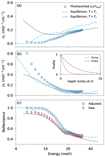
Figure 1: Conductivity (a,b) and reflectance (c) of $\text{K}_{3}\text{C}_{60}$, in equilibrium and after photoexcitation with fluence $F=3.0~{}\text{mJ}/\text{cm}^{2}$ and pump photon energy $\hbar\omega\approx 170$ meV, adapted from Budden et al. [8]. Equilibrium results are shown above and below $T_{\text{c}}=20~{}\text{K}$, at 100 K and 10 K, respectively [7]. Photoexcited results are shown at 100 K for $\Delta t=1$ ps. The photoexcited surface conductivity $\sigma_{\text{s}}$ (open circles) is inferred by assuming the profile $\mathcal{P}_{\text{exp}}$ with $\epsilon_{\infty}=5$ and $\Lambda=220$ nm [6, 8]. The distinction between the adjusted reflectance (open squares) and the raw reflectance (open diamonds) is described in the text. The inset shows $\mathcal{E}(z)$ for the pump and the probe in the linear optical regime at $\hbar\omega=6.46$ meV, each normalized to their surface value.

The optical properties reported for the photoexcited state with $T>T_{\text{c}}$ at $\Delta t=1$ ps are qualitatively similar to those of the equilibrium superconducting state. At low frequencies, photoexcitation suppresses $\sigma_{\text{s}1}$, enhances $\sigma_{\text{s}2}$, and, after an adjustment that we discuss below, causes the reported reflectance $R_{\text{adj}}$ to approach unity. The evidence for photoinduced superconductivity in $\text{K}_{3}\text{C}_{60}$ hinges on these similarities [6, 7, 8, 9].

But there is a crucial difference between the two sets of measurements. The equilibrium conductivity is spatially uniform, so for a given background relative permittivity $\epsilon_{\infty}$ there is a unique mapping from the measured complex reflection amplitude $\bar{r}$ to the quantity of interest, $\bar{\sigma}$. This is not the case for the photoinduced response, since the photoconductivity $\Delta\sigma$ is not uniform. To determine $\sigma_{\text{s}}$ uniquely from the photoexcited reflection amplitude $r$, we must also specify the conductivity profile $\mathcal{P}$ as a function of the depth $z$ from the surface. If $\mathcal{P}$ is not known independently, we must assume a model for it. Any error in this model will be passed on to $\sigma_{\text{s}}$.

Following previous practice [10, 11, 6, 7], Budden et al. [8] use a profile that we denote by $\mathcal{P}_{\text{exp}}$, which they express in terms of the refractive index as

$$n(\omega,z;\mathcal{P}_{\text{exp}})=\bar{n}(\omega)+\Delta n_{\text{s}}(\omega)\,e^{-\alpha z},$$ (1)

where $\bar{n}$ is the equilibrium refractive index, $\alpha$ is the pump attenuation coefficient, and $\Delta n_{\text{s}}$ is the photoinduced change in the refractive index at the surface. We include the label $\mathcal{P}_{\text{exp}}$ explicitly to emphasize its role in inferring $n(\omega,z;\mathcal{P}_{\text{exp}})$ from the measured $r(\omega)$. In terms of the conductivity, the profile is

$$\begin{split}\sigma(\omega,z;\mathcal{P}_{\text{exp}})&=\bar{\sigma}(\omega)+\Delta\sigma(\omega,z;\mathcal{P}_{\text{exp}}),\\ &=-i\omega\epsilon_{0}\{[n(\omega,z;\mathcal{P}_{\text{exp}})]^{2}-\epsilon_{\infty}\}.\end{split}$$ (2)

Now it is possible to determine $\sigma_{\text{s}}(\omega;\mathcal{P}_{\text{exp}})=\sigma(\omega,0;\mathcal{P}_{\text{exp}})$ from $r(\omega)$ by solving the Maxwell equations with $\mathcal{P}_{\text{exp}}$ and matching the usual electromagnetic boundary conditions at the surface [12].

The problem with this procedure is that $\mathcal{P}_{\text{exp}}$ implicitly relies on two assumptions that are both unreliable. First, it assumes that the pump absorption remains linear in the pump intensity, so that the energy density $\mathcal{E}$ absorbed by the pump decays as $\mathcal{E}\propto e^{-\alpha z}$. Second, it assumes that $n$ is linear in $\mathcal{E}$. Jointly, these assumptions imply that Eq. (2) is independent of the pump intensity. But none of these assumptions are sound at the high pump intensities used in the experiments. Indeed, the measured photoresponse consistently shows a nonlinear dependence on the incident fluence $F$ [13, 10, 14, 15, 16, 6, 17, 18, 19, 20, 21], so analyzing them in terms of the profile $\mathcal{P}_{\text{exp}}$ is not self-consistent.

And as we demonstrate here, neglecting nonlinearity can introduce errors in $\sigma_{\text{s}}(\omega;\mathcal{P}_{\text{exp}})$ that are profoundly misleading. The pump attenuation length $\Lambda=1/\alpha$ is less than a third of a typical probe attenuation length in $\text{K}_{3}\text{C}_{60}$ (see inset to Fig. 1), so the pump excites only a fraction of the probe volume and the photoinduced change in $r$ is much weaker than it would be with uniform excitation. The change $\Delta r$ is then mainly sensitive to the sheet photoconductance, $\Delta G_{\Box}=\Delta\sigma_{\text{s}}d_{\text{eff}}$, where $d_{\text{eff}}=\int dz\,\Delta\sigma(z)/\Delta\sigma_{\text{s}}$ is the effective perturbation thickness. For $\mathcal{P}_{\text{exp}}$, we get $d_{\text{eff}}=\Lambda$, independent of fluence. But this is no longer true if the photoconductivity is nonlinear, and failing to account for this will introduce error in $d_{\text{eff}}$. Any error in $d_{\text{eff}}$ will introduce a compensating error in $\Delta\sigma_{\text{s}}$, distorting $\sigma_{\text{s}}$.

The difference between the raw and adjusted reflectance in Fig. 1(c) reveals the scope for such an error. Budden et al. [8] do not report raw measurements of the photoexcited reflectance $R=|r|^{2}$, so we have deduced it from their reported $\mathcal{P}_{\text{exp}}$ and $\sigma_{\text{s}}$. What Budden et al. [8] do report is $R_{\text{adj}}$, which they compute for an interface between a diamond window (used in the measurements) and a fictitious medium with uniform $\sigma(\omega)$ that they set equal to $\sigma_{\text{s}}(\omega;\mathcal{P}_{\text{exp}})$. While the raw reflectance $R$ exceeds $\bar{R}$ by at most 3.4%, $R_{\text{adj}}$ exceeds it by as much as 15%, a discrepancy of more than a factor of 4. Note that $R_{\text{adj}}(\omega)$ is derived from $\sigma_{\text{s}}(\omega;\mathcal{P}_{\text{exp}})$, not the other way around, so any error in $\sigma_{\text{s}}$ will also appear in $R_{\text{adj}}$. If we overestimate $d_{\text{eff}}$, we will underestimate both $|\Delta\sigma_{\text{s}}|$ and $|R_{\text{adj}}-\bar{R}|$, and if we underestimate $d_{\text{eff}}$ we will overestimate them.

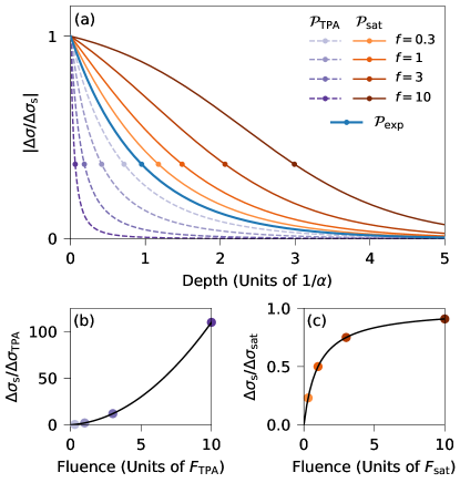
Figure 2: Local photoconductivity $\Delta\sigma$ as a function of depth from the surface (a) and pump fluence (b),(c) for two models of nonlinearity. (a) The profiles $\mathcal{P}_{\text{sat}}$ (orange, solid lines) and $\mathcal{P}_{\text{TPA}}$ (purple, dashed lines) are shown for the same four values of the normalized pump fluence $f$, indicated by markers of the corresponding color in (b) and (c) for $\mathcal{P}_{\text{TPA}}$ and $\mathcal{P}_{\text{sat}}$, respectively. The profile $\mathcal{P}_{\text{exp}}$ (blue thick line) used by Budden et al. [8] is shown for $\hbar\omega=6.46$ meV. Markers in (a) indicate the $1/e$ depth for each curve.

And as Fig. 2 makes clear, nonlinearity can cause $d_{\text{eff}}$ to change by an order of magnitude or more as the fluence increases. We show profiles for two common nonlinearities, which we discuss in more detail in the Supplemental Material [22]. In one, which we label as $\mathcal{P}_{\text{sat}}$, we assume that $\mathcal{E}\propto e^{-\alpha z}$ and that the local photoconductivity $\Delta\sigma$ saturates with $\mathcal{E}$. Defining the dimensionless fluence parameter $f=F/F_{\text{sat}}$, where $F_{\text{sat}}$ is the characteristic scale for saturation, we express $\sigma$ as [23, 24]

$$\sigma(\omega,z,f;\mathcal{P}_{\text{sat}})=\bar{\sigma}(\omega)+\Delta\sigma_{\text{sat}}(\omega)\frac{fe^{-\alpha z}}{1+fe^{-\alpha z}},$$ (3)

which yields

$$\Delta G_{\Box}(\omega,f;\mathcal{P}_{\text{sat}})=\Delta\sigma_{\text{sat}}(\omega)\Lambda\ln(1+f).$$ (4)

Note that $\Delta G_{\Box}(\omega,f;\mathcal{P}_{\text{sat}})$ continues to increase with $f$ even as $\Delta\sigma_{\text{s}}(\omega,f;\mathcal{P}_{\text{sat}})=\Delta\sigma_{\text{sat}}(\omega)f/(1+f)$ saturates. This is because $\Delta\sigma$ grows more slowly at the surface than it does in the interior as $f$ increases, which causes $d_{\text{eff}}$ to increase also. The logarithmic growth of $G_{\Box}(\omega,f;\mathcal{P}_{\text{sat}})$ with $f$ does not depend on the detailed form of the saturation in Eq. (3), since it follows from the assumption that $\mathcal{E}\propto e^{-\alpha z}$.

For the second profile, $\mathcal{P}_{\text{TPA}}$, we assume that $\Delta\sigma$ remains proportional to $\mathcal{E}$ but that the absorption is nonlinear, with a two-photon absorption (TPA) coefficient $\beta$ [22]. For simplicity, we further assume that the pump intensity has a rectangular temporal profile with duration $\tau_{\text{p}}$ and that the pump reflection coefficient $R_{\text{p}}$ remains constant. This allows us to express $\sigma$ analytically as

$$\sigma(\omega,z,f;\mathcal{P}_{\text{TPA}})=\bar{\sigma}(\omega)+\Delta\sigma_{\text{TPA}}(\omega)\frac{f(1+f)e^{-\alpha z}}{\left[1+f(1-e^{-\alpha z})\right]^{2}},$$ (5)

where now $f=F/F_{\text{TPA}}$ with $F_{\text{TPA}}=(\alpha\tau_{\text{p}}/\beta)/(1-R_{\text{p}})$. As Fig. 2(b) shows, the surface photoconductivity $\Delta\sigma_{\text{s}}(\omega,f;\mathcal{P}_{\text{TPA}})=f(1+f)\Delta\sigma_{\text{TPA}}(\omega)$ increases quadratically with $f$ when $f\gg 1$, where TPA dominates. At the same time, $d_{\text{eff}}=\Lambda/(1+f)$ decreases with $f$, which compensates for the superlinear growth of $\Delta\sigma_{\text{s}}$ and causes the sheet photoconductance,

$$\Delta G_{\Box}(\omega,f;\mathcal{P}_{\text{TPA}})=\Delta\sigma_{\text{TPA}}(\omega)\Lambda f,$$ (6)

to remain strictly proportional to $f$.

Now consider the systematic error that we introduce if we assume the wrong profile. If the true profile is $\mathcal{P}_{\text{sat}}$ but we assume it is $\mathcal{P}_{\text{exp}}$, for example, then we would infer the surface conductivity to be $\sigma_{\text{s}}(\omega,f;\mathcal{P}_{\text{sat}}\mapsto\mathcal{P}_{\text{exp}})$, where the notation $\mathcal{P}_{\text{sat}}\mapsto\mathcal{P}_{\text{exp}}$ indicates that we use the $\mathcal{P}_{\text{sat}}$ profile to compute $r(\omega)$ with a source spectrum $\sigma_{\text{s}}(\omega,f;\mathcal{P}_{\text{sat}})$, then use the $\mathcal{P}_{\text{exp}}$ profile to infer an image spectrum $\sigma_{\text{s}}(\omega;\mathcal{P}_{\text{sat}}\mapsto\mathcal{P}_{\text{exp}})$ from $r(\omega)$. The requirement that the source and image profiles yield the same $r(\omega)$ is roughly equivalent to holding $\Delta G_{\Box}=\Delta\sigma_{\text{s}}d_{\text{eff}}$ constant for $\text{K}_{3}\text{C}_{60}$, so the image transformation effectively rescales the source $\Delta\sigma_{\text{s}}$ by $d_{\text{eff}}{(\mathcal{P}_{\text{source}})}/d_{\text{eff}}{(\mathcal{P}_{\text{image}})}$. Since $d_{\text{eff}}=\Lambda$ for $\mathcal{P}_{\text{exp}}$, we divide Eq. (4) by $\Lambda$ to get

$$\Delta\sigma_{\text{s}}(\omega,f;\mathcal{P}_{\text{sat}}\mapsto\mathcal{P}_{\text{exp}})\approx\Delta\sigma_{\text{sat}}(\omega)\ln(1+f),$$ (7)

which overestimates $\Delta\sigma_{\text{s}}(\omega,f;\mathcal{P}_{\text{sat}})$ by $(1+f)\ln(1+f)/f$. Similarly, dividing Eq. (6) by $\Lambda$ gives

$$\Delta\sigma_{\text{s}}(\omega,f;\mathcal{P}_{\text{TPA}}\mapsto\mathcal{P}_{\text{exp}})\approx\Delta\sigma_{\text{TPA}}(\omega)f,$$ (8)

which underestimates $\Delta\sigma_{\text{s}}(\omega,f;\mathcal{P}_{\text{TPA}})$ by $1/(1+f)$.

Figure 3 shows the fluence dependence reported by Mitrano et al. [6] for $\Delta\sigma_{\text{s}1}(\omega;\mathcal{P}_{\text{exp}})$ in $\text{K}_{3}\text{C}_{60}$, which we use to infer the profile. The measurements reveal a clear sublinear fluence dependence that is inconsistent with the relationship expected for $\Delta\sigma_{\text{s}1}(\omega,f;\mathcal{P}_{\text{TPA}}\mapsto\mathcal{P}_{\text{exp}})$ given in Eq. (8) [22]. And as we noted earlier, the deviation from linearity is also incompatible with the assumptions that yield the $\mathcal{P}_{\text{exp}}$ profile used in the original analysis. A fit with $\Delta\sigma_{\text{s}1}(\omega,f;\mathcal{P}_{\text{sat}}\mapsto\mathcal{P}_{\text{exp}})$, however, is nearly indistinguishable from the experimental results—which means that the source function $\Delta\sigma_{\text{s}1}(\omega,f;\mathcal{P}_{\text{sat}})$, shown as a solid line in Fig. 3, is the best estimate for the true surface photoconductivity. Note that this deviates significantly from the originally reported results at all fluences, and is nearly a factor of 2 smaller than the result reported by Budden et al. [8] at $F=3.0~{}\text{mJ}/\text{cm}^{2}$.

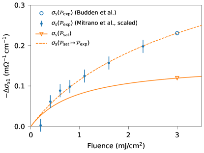
Figure 3: Least-squares fit with $\Delta\sigma_{\text{s}1}(\omega,f;\mathcal{P}_{\text{sat}}\mapsto\mathcal{P}_{\text{exp}})$ (dashed line) to the fluence dependence of $\Delta\sigma_{\text{s}1}(\omega;\mathcal{P}_{\text{exp}})$ reported by Mitrano et al. [6] (points with error bars). The fit is constrained to pass through the anchor point $\Delta\sigma_{\text{s}1}(\omega;\mathcal{P}_{\text{exp}})$ (open circle) at $F=3~{}\text{mJ}/\text{cm}^{2}$ reported by Budden et al. [8] for $\hbar\omega=6.46$ meV. We multiply the results of Mitrano et al. [6] by an overall scale factor $A$ to account for systematic differences from the results of Budden et al. [8]. Best-fit parameter values are $F_{\text{sat}}=(1.0\pm 0.5)~{}\text{mJ}/\text{cm}^{2}$ and $A=0.65\pm 0.06$ ($\chi^{2}=3.7$, $\text{d.o.f.}=5$). The solid line extrapolates the source function $\Delta\sigma_{\text{s}1}(\omega,f;\mathcal{P}_{\text{sat}})$ from its value of at $F=3~{}\text{mJ}/\text{cm}^{2}$ (open triangle).

We fix $F_{\text{sat}}$ at the value obtained from this fit and extend our analysis as a function of frequency in Fig. 4. We derive the alternative spectrum $\sigma_{\text{s}}(\omega;\mathcal{P}_{\text{sat}})$ so that its image in $\mathcal{P}_{\text{exp}}$ is equal to $\sigma_{\text{s}}(\omega;\mathcal{P}_{\text{exp}})$ reported by Budden et al. [8]. Both spectra show decreases in $\sigma_{\text{s}1}(\omega)$ and increases in $\sigma_{\text{s}2}(\omega)$, but by different amounts. Since $\Delta\sigma_{\text{s}}$ is inversely related to $d_{\text{eff}}$, $\Delta\sigma_{\text{s}}(\omega;\mathcal{P}_{\text{exp}})$ has a smaller magnitude than $\Delta\sigma_{\text{s}}(\omega,f;\mathcal{P}_{\text{sat}})$.

These quantitative differences suggest qualitatively different physical interpretations. The spectrum with $\mathcal{P}_{\text{exp}}$ looks like that of a superconductor [6, 7, 8]: $\sigma_{\text{s}1}(\omega;\mathcal{P}_{\text{exp}})$ falls to near zero below $\hbar\omega\approx 10$ meV, $\sigma_{\text{s}2}(\omega;\mathcal{P}_{\text{exp}})$ is enhanced at low frequencies, and a Drude-Lorentz fit yields a carrier relaxation rate $\gamma=0$ [22]. But the spectrum with $\mathcal{P}_{\text{sat}}$ looks like a normal metal with a photoenhanced mobility: $\sigma_{\text{s}1}(\omega,f;\mathcal{P}_{\text{sat}})$ lies well above zero at all $\omega$ and clearly increases with decreasing $\omega$ below $\hbar\omega\approx 9$ meV, while $\sigma_{\text{s}2}(\omega,f;\mathcal{P}_{\text{exp}})$ shows more moderate enhancement at low frequencies. A Drude-Lorentz fit to this spectrum yields $\hbar\gamma=1.2$ meV [22], which is about a third of the equilibrium value [9] and 4 times larger than the previously reported upper bound [7].

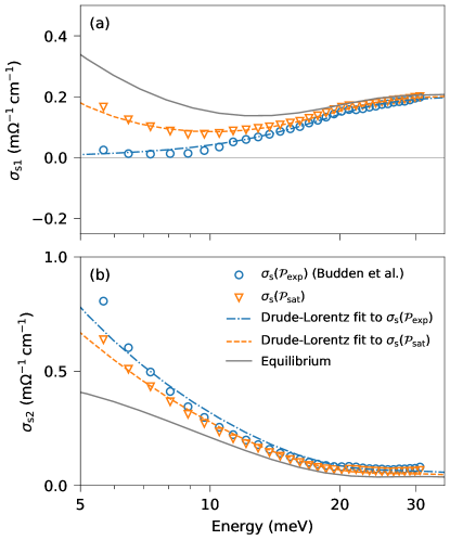
Figure 4: Real (a) and imaginary (b) parts of $\sigma_{\text{s}}$ for $F=3.0~{}\text{mJ}/\text{cm}^{2}$ with different profile assumptions. The spectrum $\sigma_{\text{s}}(\omega;\mathcal{P}_{\text{exp}})$ (open circles) reported by Budden et al. [8] and the alternative spectrum $\sigma_{\text{s}}(\omega,f;\mathcal{P}_{\text{sat}})$ (open triangles) yield the same $r(\omega)$. Lines show Drude-Lorentz fits to $\sigma_{\text{s}}(\omega;\mathcal{P}_{\text{exp}})$ (dot-dashed), $\sigma_{\text{s}}(\omega,f;\mathcal{P}_{\text{sat}})$ (dashed), and $\bar{\sigma}(\omega)$ (solid) [22].

We turn to measurements of $\text{K}_{3}\text{C}_{60}$ at higher pump fluence for further guidance. Figure 5 shows $\sigma_{\text{s}}(\omega;\mathcal{P}_{\text{exp}})$ at $F=4.5~{}\text{mJ}/\text{cm}^{2}$ reported by Buzzi et al. [9], along with the alternative spectrum $\sigma_{\text{s}}(\omega,f;\mathcal{P}_{\text{sat}})$, defined in the same way as in Fig. 4. The higher fluence produces larger changes in $\sigma_{\text{s}}$ with both profiles, driving $\sigma_{\text{s}1}$ negative for $\sigma_{\text{s}1}(\omega;\mathcal{P}_{\text{exp}})$. Buzzi et al. [9] interpreted this negative real conductivity as evidence for Higgs-mediated optical parametric amplification, generated by a rapid quench from a superconducting state. For this to work, the pump would need to both produce a transient superconducting state and quench it within 100 fs, since the experiments are conducted above the equilibrium $T_{\text{c}}$. But when we assume $\mathcal{P}_{\text{sat}}$ instead of $\mathcal{P}_{\text{exp}}$, a simpler interpretation emerges. A Drude-Lorentz fit to $\sigma_{\text{s}}(\omega,f;\mathcal{P}_{\text{sat}})$ yields $\hbar\gamma=0.6$ meV, about half the value obtained for $F=3.0~{}\text{mJ}/\text{cm}^{2}$ and 1/6 the equilibrium value [22]. Neither photoinduced superconductivity nor Higgs-mediated amplification are necessary to explain the results. At all fluences, the measurements are consistent with a relatively moderate photoinduced enhancement of the carrier mobility.

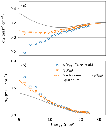
Figure 5: Profile dependence of the real (a) and imaginary (b) parts of $\sigma_{\text{s}}$ reported by Buzzi et al. [9] for $F=4.5~{}\text{mJ}/\text{cm}^{2}$. Markers and lines correspond to those in Fig. 4.

While we have focused here on $\text{K}_{3}\text{C}_{60}$ at the moment of peak response, our observations raise important interpretational questions about the entire body of experimental literature on photoinduced superconductivity. In YBa₂Cu₃O_$y$, for example, a signal associated with photoinduced superconductivity appears to show a linear dependence on the peak electric field, but the dependence is also consistent with what we have described for a saturable medium [10, 18, 22]. Furthermore, this signal is enhanced when the pump is tuned to specific phonon resonances, but if the photoconductivity saturates more easily at these resonances, the signal enhancement could be caused by changes in $d_{\text{eff}}$  instead of $\Delta\sigma_{\text{s}}$ [10, 18]. In fact, the first report of photoinduced superconductivity described a similar mechanism [13]. This work also noted that both $d_{\text{eff}}$ and the signal strength should grow logarithmically with fluence as a result of the saturation, following reasoning similar to ours [13]. Subsequent work failed to incorporate these insights, however, and needs reassessment.

There are several ways to overcome the problems that we have identified. Measurements on thin films with thickness $t\lesssim\Lambda$ would be ideal, as they would eliminate the uncertainty in $d_{\text{eff}}$. In principle, ellipsometric measurements could determine $\sigma_{\text{s}}$ and $d_{\text{eff}}$ simultaneously, although in practice this would be technically challenging. Katsumi et al. [25] has used nonlinear THz measurements to test for the existence of photoinduced superconductivity in YBa₂Cu₃O_$y$, and found none. Another approach is to examine the joint dependence of $r$ on frequency, fluence, and time to specify a parametrized model for $\sigma_{\text{s}}$, as we have described here. All of these approaches would help us to decide if the photoinduced superconductivity observed in $\text{K}_{3}\text{C}_{60}$ and other compounds is real—or if it is an artifact of nonlinear distortion.