Quantum colored lozenge tiling and entanglement phase transition

Abstract

While volume violation of area law has been exhibited in several quantum spin chains, the construction of a corresponding model in higher dimensions, with isotropic terms, has been an open problem. Here we construct a 2D frustration-free Hamiltonian with maximal violation of the area law. We do so by building a quantum model of random surfaces with color degree of freedom that can be viewed as a collection of colored Dyck paths. The Hamiltonian may be viewed as a 2D generalization of the Fredkin spin chain. Its action is shown to be ergodic within the Hilbert subspace of zero fixed Dirichlet boundary condition and positive height function in the bulk and exhibits a non-degenerate ground state. Its entanglement entropy between subsystems exhibits an entanglement phase transition as the deformation parameter is tuned. The area- and volume-law phases are similar to the one-dimensional model, while the critical point scales with the linear size of the system $L$ as $L\log L$. Similar models can be built in higher dimensions with even softer area law violations at the critical point.

In one dimension, lattice models with beyond logarithmic violation of the area law of entanglement entropy [1] have been found in a class of frustration-free (FF) models dubbed Motzkin and Fredkin spin chains with up to volume-law scaling of EE [2, 3, 4, 5, 6, 7, 8]. Despite the plethora of 1D lattice models with such violations, their 2D counterparts are yet to be discovered. In this manuscript, we give the first successful example of such a model with exotic entanglement scaling on a two-dimensional lattice. A crucial ingredient of the Motzkin and Fredkin models is that, by employing next nearest neighbor interaction and boundary condition, they allow a well-defined height representation that carries long-range entanglement which local spins could not. We are thus looking to construct a model with well defined height in 2D. An example for such a situation is the U(1) Coulomb gas phase, naturally emerged in constrained Hilbert space of fully packed dimer or loop covering models [9, 10, 11]. In Ref. [11], a first attempt was made to build two models using fully packed loops on a square lattice, but the entanglement entropy computed there obeys area law, as the ground state is a projected entangled pair state contracted by the local constraints in Hilbert space.

In Ref. [12], a 2D generalization to the Fredkin moves between lozenge tilings was first proposed as a classical stochastic model. Lozenge tilings frequently appear in the combinatorics and classical statistical mechanics literature, as a description of fully packed dimer configurations of a honeycomb lattice, and are extensively studied in the context of limit shape behavior , arctic curves [13], and the study of two dimensional KPZ growth [14]. Here, we incorporate the dynamics of [12] into a quantum Hamiltonian with projection operators that annihilate a ground state of uniform superposition of lozenge tilings. A yet richer model can be defined when the local Hilbert space is enlarged by introducing color degree of freedom to the dimers. Two- and multi-color dimer models has been studied both on the square lattice [15] and honeycomb lattice [16]. Three-color code model has also been heavily studied in the context of exactly solvable model of topological order [17], topological defect [18], and as a candidate for fault-tolerant quantum computation [19]. Recently, the dependency of entanglement entropy scaling on the number of local degrees of freedom is studied with an N-component partially integrable chain [20], which can be viewed as a low-energy effective Hamiltonian of a related quasi-2D spin ladder model [21]. In particular, the entanglement entropy of integrable excited states was shown to decompose into a part that scales only with the size of the system and one that scales also with the number of the dimensionality of local Hilbert space. In the present model, EE also decomposes into a contribution from color degrees of freedom and the height degree of freedom, the scaling of leading contribution changes qualitatively as the deformation parameter is tuned and exhibits an entanglement phase transition.

Figure 1: (a) Mapping from $s^{2}$-colored dimer coverings on honeycomb lattice to lozenge tilings with an $s$-colored line along each pair of parallel sides. (b) Convention of height change between plaquette centers and vertices of lozenges: along the positive direction of x,y,z axes height increases by 1.

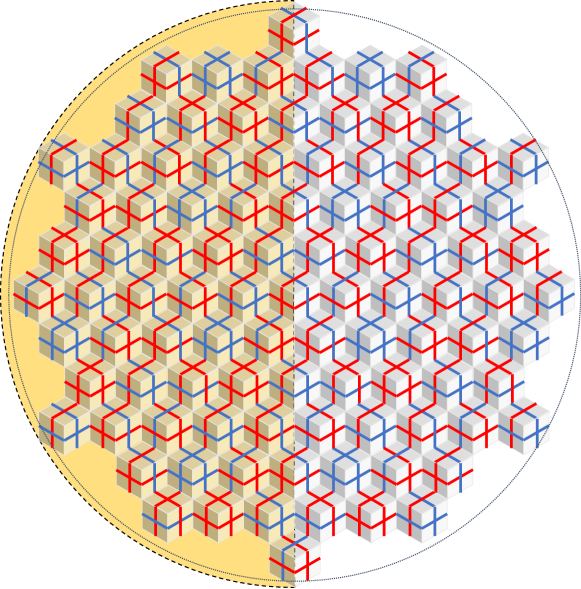
Figure 2: A coloring of the minimal volume tiling configuration of a lattice of linear size $L=20$. The dotted circle marks the boundary of the lattice corresponding to the arctic circle and the (1,1,1) plane of height 0. The dashed line marks the cut into the shaded and unshaded subsystems. The three-dimensional effect is understood with light shining against the y-axis slightly tilted downward.

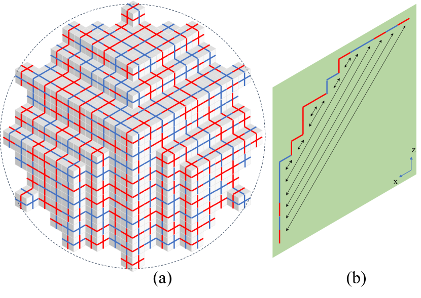
Figure 3: (a) A coloring of the maximal volume tiling configuration of a lattice of linear size $L=20$. In the thermodynamic limit, the surface approaches a dome shape. (b) One slice of the x-z plane which intersects with the maximal surface in (a) giving a colored Dyck path.

Quantum lozenge tiling. Our model of lozenge tiling on a triangular lattice $\Lambda$ can be mapped from a model of dimer covering its dual honeycomb lattice $\Lambda^{*}$, as is shown in Fig. 1 (a). On each edge of the honeycomb lattice, the local degrees of freedom are either uncovered, or covered by a dimer in one of the $s^{2}$ internal states. Furthermore, the global Hilbert space is constrained by the fully packed dimer covering condition, which means that each vertex is covered by one dimer and one dimer only. The constraint can be realized by the Hamiltonian

$$H_{0}=\sum_{\boldsymbol{r}\in\Lambda^{*}}(\sum_{i=1}^{3}n_{\boldsymbol{r},\boldsymbol{r}+\boldsymbol{e}_{i}}-1)^{2},$$ (1)

where $n_{\boldsymbol{r},\boldsymbol{r}+\boldsymbol{e}_{i}}$ is the number operator of the dimer living on the edge along the $\boldsymbol{e}_{i}$ direction at site $\boldsymbol{r}$. The constraint of fully packed dimers allows a well-defined height function on the dual triangular lattice. We adopt the height change convention as depicted in Fig. 1 (b), namely increase by 1 along the positive directions of the three axis and decrease by 1 in their opposite directions, when counting along the edge of a lozenge, accordingly the height changes by $\pm 2$ across the shorter diagonal.

A theorem by Thurston [22] says that for a triangular lattice to be tileable by lozenges, the difference between the height of two vertices on the boundary defined by the convention in Fig. 1 (b) is bounded by the minimal number of edges in a positively oriented path connecting the two vertices. The lattice of our model satisfies the stronger constraint that the difference in height along the boundary is either $0$ or $1$, by requiring consecutive edges along the boundary to rotate by an angle of $\pm\frac{\pi}{3}$. As a result, the number of three types of lozenges in the tiling, or the number of dimers with three different orientation are equal in our lattice. In Fig. 2 and 3 (a), we show two tiling configurations with a boundary inside a circle of diameter $L=20$. As the lattice size increases, the boundary of our lattice approaches the circle by filling as many hexagons in the empty space inside the circle as possible, so that in the thermodynamic or scaling limit, the lattice has a higher isotropy than the three-fold rotation symmetry. The particular choice of shape for the lattice boundary is motivated by the uniqueness of the ground state, which will become clear shortly.

The dimers in our Hilbert space have an internal degree of freedom of $s^{2}$ states mapping to a two-component coloring of the lozenges. We denote the two components with colored lines along the two edges in the middle, with each component having choices of $s$ colors.

A coloring of the minimal height configuration is shown in Fig. 2 (here the height in the bulk alternate between 0 and 1). A coloring of the maximal height configuration depicted in Fig. 3. The notion of height can be interpreted as the distance to the (1,1,1)-plane amplified by a factor of $\sqrt{3}$, if we view the tiling as a 3D pile of unit cubes, taking lozenges in three orientation as facets projected to the x-y, y-z, and z-x plane respectively.

Tracing each of the lines in Figs. 2 and 3, we see a natural Dyck path (Fig. 3(b)), a path of up/down moves that starts and ends at the same height and never goes below the initial height. While each dimer covering can have arbitrary coloring along such a path, we introduce a Hamiltonian whose ground state only allows $s-$coloring that correspond to the a proper coloring as in the Motzkin and Fredkin spin chains. These correlated colors will be responsible for the entanglement in the system.

We now construct a Hamiltonian whose ground state is a weighted superposition of such tessellations, with proper coloring. The dynamics that takes one tiling configuration to another locally different one is introduced with local interactions relating the eight pairs of configurations in (3), reminiscent of the Fredkin chain, and diagonal boundary terms that penalized configurations with height below 0 right inside the boundary. The latter takes the form

$$\begin{split}H_{\partial}=\sum_{\mathrm{edges}\in\partial\Lambda}&\sum_{c}\big{(}\ket{\includegraphics[trim=0.0pt 10.0pt 0.0pt 0.0pt,scale={0.4}]{bdrzy.pdf}}\bra{\includegraphics[trim=0.0pt 10.0pt 0.0pt 0.0pt,scale={0.4}]{bdrzy.pdf}}+\ket{\includegraphics[trim=0.0pt 10.0pt 0.0pt 0.0pt,scale={0.4}]{bdrzx.pdf}}\bra{\includegraphics[trim=0.0pt 10.0pt 0.0pt 0.0pt,scale={0.4}]{bdrzx.pdf}}+\ket{\includegraphics[trim=0.0pt 20.0pt 0.0pt 0.0pt,scale={0.4}]{bdryz.pdf}}\bra{\includegraphics[trim=0.0pt 20.0pt 0.0pt 0.0pt,scale={0.4}]{bdryz.pdf}}\\ +&\ket{\includegraphics[trim=0.0pt 10.0pt 0.0pt 0.0pt,scale={0.4}]{bdryx.pdf}}\bra{\includegraphics[trim=0.0pt 10.0pt 0.0pt 0.0pt,scale={0.4}]{bdryx.pdf}}+\ket{\includegraphics[trim=0.0pt 10.0pt 0.0pt 0.0pt,scale={0.4}]{bdrxy.pdf}}\bra{\includegraphics[trim=0.0pt 10.0pt 0.0pt 0.0pt,scale={0.4}]{bdrxy.pdf}}+\ket{\includegraphics[trim=0.0pt 20.0pt 0.0pt 0.0pt,scale={0.4}]{bdrxz.pdf}}\bra{\includegraphics[trim=0.0pt 20.0pt 0.0pt 0.0pt,scale={0.4}]{bdrxz.pdf}}\big{)},\end{split}$$ (2)

where $c$ denotes the color of the line attached to the boundary, and we used dashed line to denote the boundary of the lattice and the shaded triangle to denote the interior side of the boundary. The interaction appears in the Hamiltonian as projection operators requiring the ground state to have weighted superposition of these pairs, given by

$$H_{T}=\sum_{v\in\Lambda^{\circ}}\sum_{\vec{c},\vec{f}}\frac{1}{[2]_{q^{3}}}\ket{T_{v,f_{x},f_{y},f_{z}}^{c_{1},\cdots,c_{6}}}\bra{T_{v,f_{x},f_{y},f_{z}}^{c_{1},\cdots,c_{6}}},$$

with $[2]_{q}\vcentcolon=q+q^{-1}$, and two of the 8 terms are projectors given in terms of the following two superpositions, while the other 6 are listed in (12) in the supporting information

$$\ket{T_{v,+,+,+}^{\mathrm{r,g,b,y,p,o}}} =q^{-\frac{3}{2}}\ket{\includegraphics[trim=0.0pt 50.0pt 0.0pt 0.0pt,scale={0.4}]{hpppf.pdf}}-q^{\frac{3}{2}}\ket{\includegraphics[trim=0.0pt 50.0pt 0.0pt 0.0pt,scale={0.4}]{hpppe.pdf}},$$ (3)

$$\ket{T_{v,+,+,-}^{\mathrm{r,g,b,y,p,o}}} =q^{-\frac{3}{2}}\ket{\includegraphics[trim=0.0pt 50.0pt 0.0pt 0.0pt,scale={0.4}]{hppmf.pdf}}-q^{\frac{3}{2}}\ket{\includegraphics[trim=0.0pt 50.0pt 0.0pt 0.0pt,scale={0.4}]{hppme.pdf}},$$

where $\mathcal{L}^{\circ}$ denotes the bulk of lattice, and we have used red, green, blue, yellow, purple, and orange to represent color $c_{1},\cdots,c_{6}$ respectively to show explicitly how the Fredkin moves acts on the colors of nearest and next-nearest neighbor around vertex $v$. Note that the projectors relate between tilings where the minimal height is on the next neighbors of $v$. Therefore applying the projectors cannot make the height negative in the bulk of the lattice as long as the boundary is kept at zero height.

Note that none of the vertices in Fig. 2 overlaps with the local configurations in the first column of (3). So as long as the height of the lozenges along the boundary are set to be 0 and increase going towards inside the bulk, which is done by the boundary Hamiltonian $H_{\partial}$, the height configuration of the entire lattice are lowered bounded by 0. That boundary Hamiltonian can be written as a sum of local projection operators that penalizes local boundary configurations different from those shown in Fig. 2 and 3.

The kinetically constrained bulk Hamiltonian could fragment the space of non-negative height configurations satisfying the Fredkin condition into Krylov subspaces, but an ergodicity argument given in the Appendix C shows that all such configurations participate in the ground state superposition. So far, all the configurations between the minimal height configuration of a sharkskin surface, to the maximal height configuration of a dome are superposed to form a ground state superposition weighted by the volume underneath. Yet different colorings of lozenges in the same height configuration still live in distinct Krylov sectors. To obtain a unique ground state as a superposition of different colorings, we add a color mixing term in the Hamiltonian that require the component of color perpendicular to the convex edge where two differently oriented lozenges meet is matched and has equal probability to be in either color

$$\begin{split}H_{\Gamma}=&\sum_{v\in\Lambda^{\circ}}\sum_{n=x,y,z}\sum_{c_{1}\neq c_{2}}\ket{P_{v,n}^{c_{1},c_{2}}}\bra{P_{v,n}^{c_{1},c_{2}}}+\\ &\frac{1}{2}\left(\ket{P_{v,n}^{c_{1},c_{1}}}-\ket{P_{v,n}^{c_{2},c_{2}}}\right)\left(\bra{P_{v,n}^{c_{1},c_{1}}}-\bra{P_{v,n}^{c_{2},c_{2}}}\right),\end{split}$$ (4)

where, e.g.

$$\ket{P_{v,x}^{\mathrm{b,r}}}=\ket{\includegraphics[trim=0.0pt 25.0pt 0.0pt 0.0pt,scale={0.4}]{humxbr.pdf}},\ket{P_{v,y}^{\mathrm{b,r}}}=\ket{\includegraphics[trim=0.0pt 25.0pt 0.0pt 0.0pt,scale={0.4}]{humybr.pdf}},\ket{P_{v,z}^{\mathrm{b,r}}}=\ket{\includegraphics[trim=0.0pt 20.0pt 0.0pt 0.0pt,scale={0.4}]{humzbr.pdf}}.$$

The full Hamiltonian is now

$$H=H_{0}+H_{\partial}+H_{T}+H_{\Gamma}.$$ (5)

It is frustration free as all the terms share the common ground state

$$\ket{\mathrm{GS}}=\frac{1}{\sqrt{\mathcal{N}}}\sum_{h(\partial T)=0}\sum_{C}m(T^{C})q^{\mathcal{V}(T)}\ket{T^{C}},$$ (6)

where $\mathcal{N}$ is the normalization constant that depends only on lattice size $L$ and deformation parameter $q$, the second sum is over coloring together with the character function $m(T^{C})$ that gives one if along any cross-sectional paths in the x-y, y-z and z-x plane, the lines of lozenges match in color with their partner of the same height, and zero otherwise. The volume of a surface $\mathcal{V}(T)=\sum_{v\in\mathcal{L}}h_{v}(T)$ is defined by the sum of heights of the vertices of lozenges.

An entanglement phase transition. The entanglement entropy between two halves of the lattice (shaded and unshaded region in Fig. 2) is shown in the supplemental material to be given by

$$S_{L}(q,s)=\log s\left(\langle\mathcal{A}\rangle+L+1\right)+S_{L}(q,s=1),$$ (7)

where the leading contribution is given by the average cross-sectional area $\langle\mathcal{A}\rangle$ of the random surfaces in the ground state superposition. Its scaling property can be determined by employing the effective field theory for the normalization $\mathcal{N}$ as the partition function, as was used in the study of the dynamics of the one-dimensional Motzkin and Fredkin chains [23, 24]. A continuous field of the height configuration can be defined as a piece-wise linear function $h(x,y)$, which takes the value of $h_{v}$ at the coordinate of vertices. It is well known that the “entropy” of random surface is captured by a surface tension $\sigma(\nabla h(x,y))$ as a function of the height gradient alone [25, 26, 27]. Also taking into account the “energy” contribution from volume weighting, we get the partition function

$$Z=\int\mathcal{D}h(x,y)e^{\iint dxdy(-\sigma(\nabla h(x,y))+2(\log q)h(x,y))},$$ (8)

where $\mathcal{D}h(x,y)$ is a continuous version of $\prod_{v}\int_{0}^{+\infty}dh_{v}\equiv\prod_{v}\int_{-\infty}^{+\infty}dh_{v}\theta(h_{v})$. The discrete origin of the original problem is preserved by the requirement that the height variable $h(x,y)$ obeys a Lipschitz condition ($|\partial_{x^{\prime},y^{\prime}}\phi|\leq 1$). The surface tension is bounded (by the entropy density of dimer coverings of the Honeycomb lattice) and can be Taylor expanded as

$$\sigma(\nabla h)=\sigma_{xx}(\partial_{x}h)^{2}+\sigma_{xy}\partial_{x}h\partial_{y}h+\sigma_{yy}(\partial_{y}h)^{2}+\cdots.$$ (9)

The absence of odd order terms is clear from symmetry consideration, while higher order terms are irrelevant in the scaling limit, as will become clear shortly. To make the dependence on $L$ explicit in the free energy, we perform the substitution $x=Lx^{\prime},\quad y=Ly^{\prime}$. The free energy then becomes

$$F=\iint_{D}dx^{\prime}dy^{\prime}L^{2}\big{(}\sigma(\frac{\nabla^{\prime}\phi(x^{\prime},y^{\prime})}{L})-2(\log q)\phi(x^{\prime},y^{\prime})\big{)},$$ (10)

where $\phi(x^{\prime},y^{\prime})=h(x,y)$ now satisfy the Lipschitz property of $|\partial_{x^{\prime},y^{\prime}}\phi|\leq L$ instead, and the integration range now in the unit disk $D$. From this one can see that in the thermodynamic limit, the higher order terms in the surface tension become irrelevant. The leading Gaussian term also becomes irrelevant compare to the second term when $q\neq 1$. This is because the scaling dimension of $h$ is upperbounded by 1 due to the Lipschitz condition. In those two cases, it’s easy to see that $F$ is minimized at the “boundary” of the space of $h(x,y)$, rather than the solution of the Euler-Lagrange equation. That “boundary” is given by the Lipschitz property for the $q>1$ case, where minimization of $F$ is achieved with maximal gradient; and by the positivity for the $q<1$ case, where $F$ is minimized taking $h=0$. Thus, when $q>1$, we have $\langle\mathcal{A}\rangle=O(L^{2})$, which by (7) gives $S_{L}(q,s\neq 1)$ volume law scaling. On the other hand, for $q<1$, the cross section area $\langle\mathcal{A}\rangle$ is minimized and we have to compare this to the contributions for entropy from the colorless expression $S_{L}(q,s=1)$.

For $q=1$, the height field becomes a Gaussian free field (GFF) conditioned on staying positive. The average height in this case can be evaluated from the scaling of extremal values of the GFF without conditioning, which scales as $\log L$. Heuristically speaking, the average of the positive conditioned field needs to also scale like that in order to leave enough room for the fluctuation below it to still remain positive. This effect of “entropic repulsion” was rigorously established in Ref. [28, 29]. Therefore at the critical point of this entanglement phase transition, the contribution to the entanglement entropy from colors, at $s>1$ scales as $O(L\log L)$.

Let us now examine the colorless contribution $S_{L}(q,s=1)$. First, we note that $S_{L}(q,s=1)<(\log 2)L$. This is an immediate consequence of the fact that there are at most $2^{L}$ possible height configurations along the cross-section between the two regions. Therefore, we can conclude that for $s>1$ we have:

$$S_{L}(q,s)=\begin{cases}O(L^{2}),&q>1\\ O(L\log L),&q=1\\ O(L),&q<1\end{cases}$$ (11)

As stated above $S_{L}(q,s=1)<(\log 2)L$ for all $q>0$, implying that the area law always holds for $s=1$. It is interesting to note that the difference between the colored and colorless case is most drastic for the $q>1$ phase. In this case the probability is narrowly concentrated near the maximal volume configuration, and surface fluctuations are suppressed. We therefore expect that the contribution to $S_{L}(q,s=1)$ from such fluctuations does not scale with system size. This is the hallmark of a strong confinement of the fluctuating degrees of freedom to a small region near the center, and would yield a $O(1)$ contribution to the entropy besides the trivial $O(L)$ entropy from cutting horizontal lozenges into halves. As a side remark, one can perform q-deformations to the Hamiltonian and obtain entanglement entropy of q-weighted superposition from results in q-enumerations of lozenge tilings [30].

Higher dimensions. Without constructing explicit models, we make a prediction of how our recipe with the three ingredients of next-neighbor interaction, color matching and boundary condition could result in area violations of entanglement entropy in higher dimensions. Three-dimensional random tilings such as rhombohedra tiling are surveyed in the Ref.[31], along with the behavior of the fluctuation of their height functions in the “perpendicular space”. In dimensions larger than 3, the fluctuation of a Gaussian free field are of order 1, which can be seen from a momentum space integration to obtain the Green’s function. Conditioned on staying positive due to the boundary condition and next-neighbor interaction, the average height scales as $\sqrt{\log L}$ as a result of the entropic repulsion [28]. Therefore, at $q=1$, entanglement entropy of the ground state of such models scales with the $d-1$ dimensional cross-sectional area between subsystems as $L^{d-1}\sqrt{\log L}$. When $q\neq 1$, the linear term in the free energy (10) still outweighs the gradient term, making the entanglement scaling on the two side of the critical point still obeying area and volume law respectively.

Final remarks. It is quite clear that our toy Hamiltonian, despite being completely local, would not be easy to create experimentally. The most difficult step is to find a mechanism for the next-neighbor interaction and internal color degree of freedom to emerge from the microscopic level. Nonetheless, significant progress has been made realizing three-body interactions both in cold atom experiments [32], and in proposals for real materials [33]. An even harder obstacle to expermintal realization is the gap scaling: in the regime of volume entanglement we expect the gap to vanish very rapidly in the thermodynamic limit, as is the case in the 1D area deformed Motzkin and Fredkin chains [34, 8, 35]. The scaling of the gap in the system will be considered in other projects. Another direction worth exploring is how to generate such states dynamically, i.e. as the output of a quantum circuit.

It is interesting to explore possible holographic tensor network representations of the ground states for various $q$, as was done in the 1D case for Motzkin chain [36]. An interesting direction is considering how the presence of defects on the local constraints would affect the entanglement and if it is possible to define a nearest neighbor Hamiltonian resembling the Motzkin interaction in the presence of such defects.

Appendix A More details of the Hamiltonian

The other six projectors not shown in (3) are listed below:

$$\ket{T_{v,+,-,+}^{\mathrm{r,g,b,y,p,o}}} =q^{-\frac{3}{2}}\ket{\includegraphics[trim=0.0pt 40.0pt 0.0pt 0.0pt,scale={0.4}]{hpmpf.pdf}}-q^{\frac{3}{2}}\ket{\includegraphics[trim=0.0pt 40.0pt 0.0pt 0.0pt,scale={0.4}]{hpmpe.pdf}},$$ (12)

$$\ket{T_{v,+,-,-}^{\mathrm{r,g,b,y,p,o}}} =q^{-\frac{3}{2}}\ket{\includegraphics[trim=0.0pt 40.0pt 0.0pt 0.0pt,scale={0.4}]{hpmmf.pdf}}-q^{\frac{3}{2}}\ket{\includegraphics[trim=0.0pt 40.0pt 0.0pt 0.0pt,scale={0.4}]{hpmme.pdf}},$$

$$\ket{T_{v,-,+,+}^{\mathrm{r,g,b,y,p,o}}} =q^{-\frac{3}{2}}\ket{\includegraphics[trim=0.0pt 35.0pt 0.0pt 0.0pt,scale={0.4}]{hmppf.pdf}}-q^{\frac{3}{2}}\ket{\includegraphics[trim=0.0pt 35.0pt 0.0pt 0.0pt,scale={0.4}]{hmppe.pdf}},$$

$$\ket{T_{v,-,+,-}^{\mathrm{r,g,b,y,p,o}}} =q^{-\frac{3}{2}}\ket{\includegraphics[trim=0.0pt 35.0pt 0.0pt 0.0pt,scale={0.4}]{hmpmf.pdf}}-q^{\frac{3}{2}}\ket{\includegraphics[trim=0.0pt 35.0pt 0.0pt 0.0pt,scale={0.4}]{hmpme.pdf}},$$

$$\ket{T_{v,-,-,+}^{\mathrm{r,g,b,y,p,o}}} =q^{-\frac{3}{2}}\ket{\includegraphics[trim=0.0pt 40.0pt 0.0pt 0.0pt,scale={0.4}]{hmmpf.pdf}}-q^{\frac{3}{2}}\ket{\includegraphics[trim=0.0pt 40.0pt 0.0pt 0.0pt,scale={0.4}]{hmmpe.pdf}},$$

$$\ket{T_{v,-,-,-}^{\mathrm{r,g,b,y,p,o}}} =q^{-\frac{3}{2}}\ket{\includegraphics[trim=0.0pt 50.0pt 0.0pt 0.0pt,scale={0.4}]{hmmmf.pdf}}-q^{\frac{3}{2}}\ket{\includegraphics[trim=0.0pt 50.0pt 0.0pt 0.0pt,scale={0.4}]{hmmme.pdf}}.$$

Appendix B Entropy and Schmidt decomposition

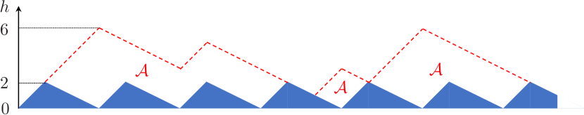
Figure 4: Cross-sectional view of the random faceted dome surface (red dashed line). The cross-sectional area $\mathcal{A}$ is defined as the sum of the height difference between the red dashed line and the blue zigzag denoting the lowest height surface in Fig. 2.

Choosing a vertical cut across the center, the Schmidt decomposition of the ground state (6) can be written as

$$\ket{\mathrm{GS}}=\sum_{\vec{h};\vec{c}}\sqrt{\frac{M_{\vec{h}}^{2}}{\mathcal{N}}}\ket{T^{\vec{c}}_{\vec{h}}}_{\mathrm{L}}\otimes\ket{T^{\vec{c}}_{\vec{h}}}_{\mathrm{R}},$$ (13)

where

$$\ket{T^{\vec{c}}_{\vec{h}}}_{\mathrm{L(R)}}=\frac{1}{\sqrt{M_{\vec{h}}}}\sideset{}{{}^{\prime}}{\sum}q^{\mathcal{V}_{\mathrm{L(R)}}(T^{C})}\ket{T^{C}}_{\mathrm{L(R)}}$$ (14)

are normalized wave functions of the left (resp. right) subsystems, including half horizontal lozenges wherever the cut intersects them, and the primed sum is a shorthand notation for summing over tiling configurations in the left (resp. right) subsystem with height profile $\vec{h}$ on the middle boundary and coloring $\vec{c}$ of the dangling lozenges with one or two of their color components entangled in the other subsystem. The total number of entangled pairs of color components $N_{C}$ is a constant proportional to the size of the lattice, and the unmatched color pairs is fixed by the height profile along the cut. The latter can be determined by noticing that raising a local height by any of the eight moves in (3), the number of entangled pairs across the cut increases by 3, one from the pair of color matching lines in the x-y plane of vertical lozenges, and two from the two lines in x and y direction of the horizontal lozenge that left and right subsystem share. This amounts to $\mathcal{A}(T)+L+1$ , with $\mathcal{A}$ defined as the cross-sectional area of cut in the $(1,-1,0)$ plane, i.e. the sum over heights along the cut subtracting that of the minimal height tiling. So we have

$$M^{2}_{\vec{h}}=s^{N_{C}-\mathcal{A}(\vec{h})-L-1}\sum_{\vec{h}(T|_{\mathrm{cut}})=\vec{h}}q^{2\mathcal{V}(T)},$$ (15)

where the sum is over a colorless tiling $T$ with height $\vec{h}$ along the cut, and

$$\mathcal{N}=\sum_{\vec{h}}s^{\mathcal{A}(\vec{h})+L+1}M^{2}_{\vec{h}}\equiv s^{N_{C}}\sum_{T}q^{2\mathcal{V}(T)}.$$ (16)

The Schmidt coefficients

$$p_{\vec{h},\vec{c}}=\frac{M^{2}_{\vec{h}}}{\mathcal{N}}=s^{-\mathcal{A}(\vec{h})-L-1}p_{\vec{h}},$$ (17)

can be factorized into the product of a constant conditional probability of having a particular coloring of the dangling pairs matched in color across the cut, and the marginal probability $p_{\vec{h}}\equiv\sum_{\vec{c}}p_{\vec{h},\vec{c}}$ for a uncolored random dome to have height profile $\vec{h}$ along the cut. This results in a decomposition of the entanglement entropy into contributions from color and height degrees of freedom, with the former given in terms of average cross-sectional area of a random dome surface

$$\begin{split}S_{L}(q,s)=&-\sum_{\vec{h}}s^{\mathcal{A}(T)+L+1}p_{\vec{h}}\log p_{\vec{h}}\\ =&\log s\left(\langle\mathcal{A}\rangle+L+1\right)+S_{L}(q,s=1),\end{split}$$ (18)

which decomposes the entanglement entropy into contributions from the internal degree of freedom of coloring in terms of the average cross-sectional area of uncolored random domes, and the a contribution $S_{L}(q,s=1)$ from the fluctuation of the shape of uncolored random domes.

Appendix C Ergodicity of the Hamiltonian and uniqueness of ground state

Figure 5: (a)The three next neighbor configurations that forbid the local maximal height $h_{M}$ to be lowered, corresponding to two next neighbors along the same axis having the same maximal height. The heights of surrounding sites are marked relative the $h_{M}$. (b) The six local configurations corresponding to the turning point along the boundary of a plateau of maximal height. (c) Two addional local configurations that allow the maximal height $h_{M}$ to be lowered even if it’s neither isolated nor on the boundary of a plateau.

We establish the ergodicity of the Hamiltonian in two steps: First by showing the tiling Hamiltonian $H_{T}$ relates all color-blind tiling configurations to the sharkskin surface in Fig. 2, corresponding to the minimal height configuration. Then since the color mixing Hamiltonian $H_{\Gamma}$ mixes the coloring of each neighboring pairs in this configuration, following the reversed path of removal of cubes to the sharkskin surface, the distant entangled pairs in the original random dome surfaces can have any allowed coloring with a total of $s^{N_{C}}$ choices.

Given any tiling configuration, there must be a site on the triangular lattice $\Lambda$ with maximal height $h_{M}$, which may not necessarily be unique. The heights of its nearest neighbors alternate between $h_{M}-1$ and $h_{M}-2$, but the next-nearest neighbors can either have height $h_{M}$ or $h_{M}-3$. If one of the next-nearest neighbours has also height $h_{M}$, we say our maximal height site is part of a plateau (see Fig. 5 (a,b) for illustration of boundaries of such plateau), otherwise it is an isolated maximum. The isolated maxima are removable by one of the eight moves in (3) and (12). Maxima sites in the bulk of a plateau (i.e. those with all six next-nearest neighbours are at the same height $h_{M}$) are not removable. Maxima sites on a plateaux boundary are only removable if they are at the corner of a plateau boundary where there is a turn (Fig. 5 (b)), as along a straight line of boundary both sides in the direction of the boundary are not in the right configuration to allow one of the Fredkin moves, since the next-nearest neighbors are both of the same height (Fig. 5 (a)). So, given any boundary of a plateau, we can always reduce the volume of a surface by starting with removing the unit cubes on the (convex) corners of plateaux boundaries, after which new corners will appear, so that the procedure keeps going. The only scenario such a procedure terminates is when the boundary forms a straight line with the plateau extending to the boundary of the lattice. In that case, both sides of the straight line have the same constant height as the boundary, meaning we have arrived at the lowest height configuration.

Now that we have shown all tiling configurations with the same boundary setting are related the the sharkskin surface, the unique ground state of the Hamiltonian, which first of all, has to comply with that boundary condition, must be a superposition of all the tiling configurations weighted by the volume under the surface, in order to be annihilated by all the projection operators enforcing weighted pairing between locally different configurations.