A Partially Functional Linear Modeling Framework for Integrating Genetic, Imaging, and Clinical Data

Abstract

This paper is motivated by the joint analysis of genetic, imaging, and clinical (GIC) data collected in the Alzheimer’s Disease Neuroimaging Initiative (ADNI) study. We propose a regression framework based on partially functional linear regression models to map high-dimensional GIC-related pathways for Alzheimer’s Disease (AD). We develop a joint model selection and estimation procedure by embedding imaging data in the reproducing kernel Hilbert space and imposing the $\ell_{0}$ penalty for the coefficients of genetic variables. We apply the proposed method to the ADNI dataset to identify important features from tens of thousands of genetic polymorphisms (reduced from millions using a preprocessing step) and study the effects of a certain set of informative genetic variants and the baseline hippocampus surface on thirteen future cognitive scores measuring different aspects of cognitive function. We explore the shared and different heritablity patterns of these cognitive scores. Analysis results suggest that both the hippocampal and genetic data have heterogeneous effects on different scores, with the trend that the value of both hippocampi is negatively associated with the severity of cognition deficits. Polygenic effects are observed for all the thirteen cognitive scores. The well-known APOE4 genotype only explains a small part of the cognitive function. Shared genetic etiology exists, however, greater genetic heterogeneity exists within disease classifications after accounting for the baseline diagnosis status. These analyses are useful in further investigation of functional mechanisms for AD evolution.

Keywords: Clinical; Genetics; Imaging; Non-asymptotic error bounds; Partially functional linear regression; Reproducing kernel Hilbert space; Sparsity.

1 Introduction

Alzheimer’s disease (AD) is a chronic neurodegenerative disease that causes degeneration of brain cells and decline in thinking, behavioral and social skills. It involves cognitive impairment with substantial between-patient variability in clinical presentation as well as the burden and distribution of pathology. Such clinicopathologic heterogeneity is both challenges and opportunities for carrying out systematic and biomarker-based studies to refine our understanding of AD biology, diagnosis, and management (Duong et al., 2022). AD has complex pathophysiological mechanisms which are not completely understood. The advances in biomarker identification, including genetic and imaging data, may improve the identification of individuals at risk for AD before symptom onset.

The primary aim of this study is to use Genetic, Imaging, and Clinical (GIC) variables from the ADNI study to map the biological pathways of AD related phenotypes of interest (e.g., cognition, intelligence, disease stage, impairment score, and progression status) (Sudlow et al., 2015; Elliott et al., 2018). It may provide insights into the biological process of brain development, healthy aging, and disease progress. For instance, it is great interest to integrate GIC to elucidate the environmental, social, and genetic etiologies of intelligence and to delineate the foundation of intelligence differences in brain structure and functioning (Deary et al., 2022). Moreover, many brain-related disorders including AD are often caused by a combination of multiple genetic and environmental factors, while being the endpoints of abnormality of brain structure and function (Shen and Thompson, 2019; Zhao et al., 2019; Knutson et al., 2020). A thorough understanding of such neuro-biological pathways may lead to the identification of possible hundreds of risk genes, environmental risk factors, and brain structure and function that underline brain disorders. Once such identification has been accomplished, it is possible to detect these risk genes and factors and brain abnormalities early enough to make a real difference in outcome and to develop their related treatments, ultimately preventing the onset of brain-related disorders and reducing their severity.

We extract clinical, imaging and genetic variables from the ADNI study. It includes cognitive scores for quantifying behavior deficits, ultra-high dimensional genetic covariates, other demongraphic covariates at baseline and brain structures using brain imaging. As previous studies have shown that the hippocampus is particularly vulnerable to AD pathology and has become a major focus in AD (Braak and Braak, 1998), we characterize the exposure of interest, hippocampal shape, by the left/right hippocampal morphometry surface data as a 100$\times$150 matrix. We give a detailed data description in Section 2. Exploring how human brains and genetics connect to human behavior is a central goal in medical studies. We are interested in how hippocampal shape and genetics are associated with future cognition deficits in Alzheimer’s study. The special data structure of these GIC variables presents new challenges for mapping the GIC pathway. First, conventional statistical tools that deal with scalar exposure are not applicable to 2D high-dimensional hippocampal imaging measures. Second, the dimension of the genetic covariates is much larger than the sample size. An effective statistical method which can exploit the 2D hippocampal surface data and the ultra-high dimensional genetic data to map the GIC pathway is urgently needed.

The literature on analysis for imaging genetics has proliferated over the past decade. There have roughly four categories of statistical methods for the analysis. The first is identifying genetic risk factors for scalar phenotype of interest through genome-wide association study, such as Carrasquillo et al. (2009), Bertram and Tanzi (2012) and Lo et al. (2019). The second is analysis of neuroimaging data, ranging from acquiring raw neuroimaging data, locating brain activity, to predicting psychological, psychiatric or cognitive states (Lindquist, 2008). The statistical tools for detecting association between scalar phenotype of interest and imaging data include voxelwize regression Zhou et al. (2014), functional data analysis approach (Reiss and Ogden, 2010), and tensor regression models that exploits the array structure in imaging data (Zhou et al., 2013; Wang et al., 2017; Li and Zhang, 2021) The third is investigating the effects of genetic variations on imaging phenotypes. Blokland et al. (2012) and Zhao et al. (2019) used imaging traits as phenotype and quantify the effects of genetics on the structure and function of the human brain. The forth is mapping biological pathways linking genetics and imaging data to neuropsychiatric disorders and examining the joint effects of both genetic risk factors and imaging data, which remains challenging and has not been studied systematically compared to the above three categories (Zhu et al., 2022). Most of the exiting methods first extracted features from the imaging data and focused on the effects of the obtained features and genetic data, see Dukart et al. (2016), Ossenkoppele et al. (2021), Cruciani et al. (2022) and references therein, which ignored the rich smoothness information in the imaging data.

To map GIC-related pathways, we consider a high-dimensional Partially Functional Linear Model (PFLM) as follows:

$$Y_{i}=\alpha+X_{i}^{T}\beta+\int_{\mathcal{T}}Z_{i}(t)\xi(t)dt+\epsilon_{i}~{}~{}~{}\mbox{for}~{}~{}i=1,\ldots,n,$$ (1)

where $Y_{i}$ is a continuous phenotype of interest for subject $i$, $X_{i}\in\mathcal{X}$ is a $p\times 1$ vector of genetic and environmental variables, and $Z_{i}(t)\in L_{2}(\mathcal{T})$ is an imaging (or functional) predictor over a compact set $\mathcal{T}$. Moreover, $\alpha$ is the intercept term, $\beta$ is a $p\times 1$ vector of coefficients, $\xi(t)$ is an unknown slope function, which is assumed to be in a reproducing kernel Hilbert space (RKHS) $\mathcal{H}$, and $\epsilon_{i}$s are measurement errors. We consider the case that the dimension of $\beta$ is either comparable to or much larger than the sample size $n$ and $\xi(t)$ is an infinite dimensional function. Our statistical problem of interest is to make statistical inference on $\beta$ and $\{\xi(t):t\in\mathcal{T}\}$. As illustrated in Fig 1, there exist genetic and clinical confounders which affect both hippocampal shape and behavioral deficits (Selkoe and Hardy, 2016). Compared to the classical high dimensional linear model that only considers the genetic data, the inclusion of imaging exposure $\xi(t)$ has two important implications for the ADNI dataset. First, model (1) is able to quantify the direct effects of the confounders by controlling for the imaging exposure. Second, model (1) investigate the influence of the imaging exposure while controlling for the confounders and preserving the structure of the imaging data.

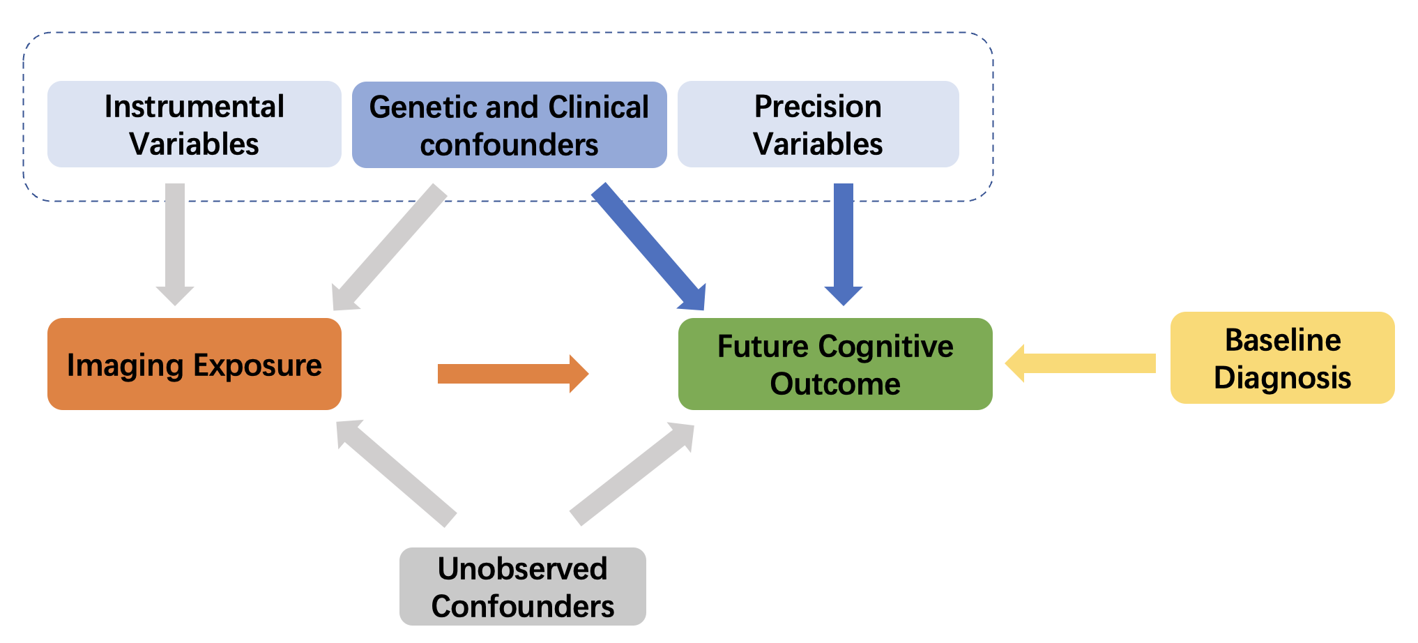
Figure 1: Directed acylic graph showing potential relationships between the genetic data, the imaging data and the future outcome. The colored arrows denote the associations of interest.

There is scarce literature on PFLM with high dimensional scalar covariates with a few exceptions. Kong et al. (2016) studied PFLM in high dimension, in which the dimension of scalar covariates was allowed to diverge with $n$. Yao et al. (2017) developed a regularized partially functional quantile regression model, while allowing the number of scalar predictors to increase with the sample size. Ma et al. (2019) focused on the partial functional partial regression model in ultra-high dimensions with a diverging number of scalar predictors. All of the above three methods consist of three steps, representing the functional predictors by using their leading functional principal components (FPCs), reducing PFLM to a standard high dimensional linear regression model, and selecting important features through the smoothly clipped absolute deviation (SCAD) penalty (Fan and Li, 2001). Therefore, existing approaches rely heavily on the success of the FPCA approach (Wang et al., 2016).

In this paper, we focus on the high dimensional PFLM (1), develop estimation method for model selection and estimation, investigate theoretical properties of both the functional and scalar estimators, and apply the proposed method to analyze the ADNI dataset. We use the RKHS framework (Yuan and Cai, 2010; Cai and Yuan, 2012; Li and Zhu, 2020) and impose the roughness penalty on the functional coefficient. The success of the existing FPCA-based methods relies on the availability of a good estimate of the functional principal components for the functional parameter, and may not be appropriate if the functional parameter cannot be represented effectively by the leading principals of the functional covariates (Yuan and Cai, 2010). On the other hand, the truncation parameter in the FPCA changes in a discrete manner, which may yield an imprecise control on the model complexity, as pointed out in Ramsay and Silverman (2005). Furthermore, we impose the $\ell_{0}$ penalty on the scalar predictors due to the fact that the $\ell_{0}$ penalty function is usually a desired choice among the penalty functions as it directly penalizes the cardinality of a model and seeks the most parsimonious model explaining the data. However, it is nonconvex and the solving of an exact $\ell_{0}$-penalized nonconvex optimization problem involves exhaustive combinatorial best subset search, which is NP-hard and computationally challenging (Zhao et al., 2019). We modify the computational algorithm in Huang et al. (2018) to deal with the above difficulty and to accommodate the functional predictor. Specifically, we proceed in three steps: (i) profiling out the functional part by using the Representer theorem; (ii) simultaneously identifying the important features and obtaining scalar estimates; and (iii) plugging the scalar estimates into the loss function to derive the functional estimate. Meanwhile, we adapt the test statistic in Li and Zhu (2020) to test the significant of the functional variable. The implementation R code with its documentation is available as an online supplement.

Numerically, the proposed method is tested carefully on the simulated data. We also provide theoretical properties of the estimators, including the error bounds of, the asymptotic normality of the estimates of the nonzero scalar coefficients, and the null limit distribution of the test statistic designed to test the nullity of the functional variable. We apply PFLM to the ADNI dataset and carry out a throughout association analysis between genetics, hippocampus and cognitive deficit. Different from the existing analysis targeted to one or several cognitive measures, the proposed method examines the joint effects of genetics and hippocampus on 13 cognitive variables observed at 12 months after baseline measurements, that measure different aspects of the cognitive function, and explore the shared and different heritablity patterns of the 13 cognitive scores. We also investigate the effect of the baseline diagnoiss information on future cognitive outcome, denoted by the yellow arrow in Fig 1. Analysis results suggest that both the hippocampal and genetic data have heterogeneous effects on different scores. In general, the value of both hippocampi is negatively associated with the severity of cognition impairments. Polygenic effects are observed for all the 13 cognitive scores and shared genetic etiology exists. The strong genetic influence is only partly attributed to the well-known APOE4 genotype, and the baseline diagnosis status explains a larger part of the cognitive function. There also exist strong shared genetic effect beside the effect of the APOE4 gene. However, greater genetic heterogeneity exists within disease classifications after accounting for the baseline diagnosis status, These analyses are useful in further investigation of functional mechanisms for AD evolution.

The rest of this paper is organized as follows. Section 2 includes a detailed data and problem description. Section 3 describes our estimation procedure. Section 4 presents Monte Carlo simulation studies to assess the finite sample performance of the proposed method. Section 5 provides a detailed data analysis on the ADNI study. Theoretical properties of our estimators and their proofs, additional simulation and real data analysis results can be found in the supplementary material.

2 Data and Problem Description

The ADNI is a large-scale multisite neuroimaging study that has collected clinical, imaging, genetic and cognitive data at multiple time points from cognitive normal (CN) subjects, subjects with mild cognitive impairment (MCI), and AD patients. It supports the investigation and development of treatments that may slow or stop the progression of AD. The primary goal of ADNI is to test whether genetic, structural and functional neuroimaging, and clinical data can be integrated to assess the progression of MCI and early AD.

We constructed a data set from the ADNI database (adni.loni.usc.edu). It consists of 606 subjects with 113 AD patients, 316 patients with mild cognitive impairment (MCI), and 177 normal controls (NC). It also includes a set of demographic variables including Age, Gender(0=Male; 1=Female), Handedness(0=Right; 1=Left), Retirement (0=No; 1=Yes), and Years of education. The average age is 75.6 years old with standard deviation 6.6 years, and the average years of education is 15.7 years with standard deviation 2.9 years. Among all the subjects, 361 are male, and 245 are female; 562 are right-handed, and 44 are left-handed; 497 are retired and 109 are not.

We extracted GIC variables as follows. First, we extracted 13 cognitive variables at 12 months after the onset of ADNI for measuring the severity of the cognitive impairment (Battista et al., ; Grassi et al., 2019). See Table S1 in the supplementary material for a summary of the abbreviations of these variables. Fig 2 presents the correlations between these scores. Among them, DIGITSCORE, RAVLT.learning, RAVLT.immediate, LDELTOTAL, and MMSE are positively correlated with lower values indicating more severe cognitive impairment, whereas CDRSB, FAQ, RAVLT.forgetting, RAVLT.perc.forgetting, TRABSCOR, ADAS11, ADAS13, and ADASQ4 are negatively correlated with higher values indicating more severe cognitive impairment. Second, we calculated the hippocampal morphometry surface measure as a $100\times 150$ matrix, each element of which is a continuous variable, representing the radial distance from the corresponding coordinate on the hipppocampal surface to the medial core of the hippocampus. Such hippocampus surface measures may provide more subtle indexes compared with the volume differences in discriminating between patients with Alzheimer’s and healthy control subjects (Li et al., 2007). Third, we extracted ultra-high dimensional genetic markers and other demongraphic covariates at baseline. There are $6,087,205$ genotyped and imputed single-nucleotide polymorphisms (SNPs) on all of the 22 chromosomes.

The clinical spectrum of AD can be very heterogeneous. Specifically, there are two main clinical syndromes including Amnestic AD with significant impairment of learning and recall and non-amnestic AD with impairment of language, visuospatial or executive function (McKhann et al., 2011). These scores measure different functions and they may lack sensitivity in different stages of AD. For example, the detection of changes of ADAS11 and ADAS13 is limited by a substantial floor effect (Hobart et al., 2013), whereas CDRSB lacks sensitivity to detect changes in very early stage of AD (de Aquino, 2021).

Little is known about the genetic architecture of these cognitive scores and the genetic-imaging-clinical (GIC) pathway for AD. We are particularly interested in the following scientific questions:

• (Q1) How to quantify the joint effect of genetic and imaging markers on the thirteen cognitive scores?

• (Q2) How to measure the shared and different heritability patterns of the thirteen different cognitive scores with/without correcting APOE4, which is supposed to be the stongest risk factor gene for AD?

• (Q3) How do the estimates and heritability patterns of thirteen different cognitive scores differ with/without correcting baseline diagnosis information?

We use model (1) to address (Q1)-(Q3) below.

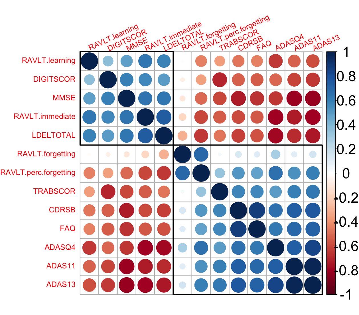
Figure 2: ADNI data analysis: correlations between the 13 cognitive variables.

3 Estimation and Inference Procedures

3.1 Estimation Algorithm

In this subsection, we develop an estimation method for model (1). First, we need to introduce some notation. Denote $\mathbf{Y}=(Y_{1},\ldots,Y_{n})^{T}$, $\mathbf{X}=(X_{1}^{T},\ldots,X_{n}^{T})^{T}$, $\mathbf{Z}=(Z_{1},\ldots,Z_{n})^{T}$, and $\boldsymbol{\epsilon}=(\epsilon_{1},\ldots,\epsilon_{n})^{T}$. Denote the true value of $\xi$ and $\beta$ as $\xi^{*}$ and $\beta^{*}$, respectively. Let $S=\{1,2,\ldots,p\}$. For any $A$ and $B\subseteq S$ with length $|A|$ and $|B|$, denote $\beta_{A}=(\beta_{i},i\in A)\in\mathbb{R}^{|A|}$. Denote $\beta|_{A}\in\mathbb{R}^{p}$ be a vector with its $i$-th element $(\beta|_{A})_{i}=\beta_{i}1(i\in A)$, where $1(\cdot)$ is the indicator function. Let $\|\beta\|_{k,\infty}$ be the $k$th largest elements in absolute value. Denote $\|\cdot\|_{0}$ as the $\ell_{0}$ norm that calculates the number of nonzero elements of a vector. Let $\|\cdot\|_{2}$ be the $\ell_{2}$-norm such that $\|\beta\|^{2}_{2}=\sum_{i=1}^{p}\beta_{i}^{2}$ and $\|\cdot\|_{L_{2}}$ be the $L_{2}$-norm such that $\|\xi\|^{2}_{L_{2}}=\int_{\mathcal{T}}\xi^{2}(t)dt$. Thus, we assume throughout $E(X)=0$, $E\{Z(t)\}=0$ and $E(Y)=0$, and therefore the intercept term can be ignored. In practice, we assume that the response $Y_{i}$ and the predictors $X_{i}$ and $Z_{i}(\cdot)$ are all mean centered such that $n^{-1}\sum_{i=1}^{n}Y_{i}=0$, $n^{-1}\sum_{i=1}^{n}X_{i}=\mathbf{0}$, and $n^{-1}\sum_{i=1}^{n}Z_{i}(\cdot)=0$.

We use the least-squares loss to estimate the functional and scalar coefficients. Due to the infinite-dimensional functional coefficient and high dimensional scalar coefficients, regularizations are needed for estimating both $\xi(t)$ and $\beta$. Similar to Yuan and Cai (2010) and Cai and Yuan (2011), the functional coefficient $\xi^{*}$ is assumed to reside in a RKHS $\mathcal{H}(K)$ with a reproducing kernel $K$. The RKHS roughness penalty is imposed on the functional parameter, while the $\ell_{0}$ penalty is imposed on the scalar parameters following a similar spirit of Huang et al. (2018). Therefore, we solve the following minimization problem

$$\min_{\beta\in\mathbb{R}^{p},\xi\in\mathcal{H}}(2n)^{-1}\sum_{i=1}^{n}\left[Y_{i}-\left(X_{i}^{T}\beta+\int_{\mathcal{T}}Z_{i}(t)\xi(t)\mathrm{d}t\right)\right]^{2}\quad\text{subject to }\|\beta\|_{0}\leq J,~{}\|\xi\|_{\mathcal{H}}^{2}\leq\widetilde{J},$$

where $J>0$ controls the sparsity level of $\beta$ and $\widetilde{J}>0$ controls the smoothness level of $\xi$. Consider the Lagrangian form of the above minimization problem

$$\min_{\beta\in\mathbb{R}^{p},\xi\in\mathcal{H}}\Biggr{\{}(2n)^{-1}\sum_{i=1}^{n}\left[Y_{i}-\left(X_{i}^{T}\beta+\int_{\mathcal{T}}Z_{i}(t)\xi(t)\mathrm{d}t\right)\right]^{2}+\tau\|\beta\|_{0}+{0.5\lambda}\|\xi\|_{\mathcal{H}}^{2}\Biggr{\}},$$ (2)

where $\tau$ and $\lambda$ are the Lagrange multipliers. To solve the minimization problem (2), the following Representer theorem is very useful.

Theorem 1.

For any $\beta\in\mathbb{R}^{p}$, there exists a parameter vector $\mathbf{c}({\beta})$ such that

$$\widehat{{\xi}}({\beta})=\sum_{i=1}^{n}c_{i}(\beta)(KZ_{i})$$ (3)

where $c_{i}(\beta)$ is the $i$-th component of $\mathbf{c}({\beta})$ and $Kf:=\int_{\mathcal{S}}K(\cdot,t)f(t)\mathrm{d}t$ for $f\in L_{2}(\mathcal{T})$.

Define $\boldsymbol{\Sigma}_{ii^{\prime}}=\iint_{\mathcal{S}\times\mathcal{S}}Z_{i}(s)K(s,t)Z_{i^{\prime}}(t)\mathrm{d}s\mathrm{d}t$ as the $(i,i^{\prime})$-th entry of $\boldsymbol{\Sigma}$. The objective function in (2) can be written in matrix form as

$$(2n)^{-1}\left\|\mathbf{Y}-\mathbf{X}\beta-\boldsymbol{\Sigma}\mathbf{c}\right\|_{2}^{2}+\tau\|\beta\|_{0}+{0.5\lambda}\mathbf{c}^{T}\boldsymbol{\Sigma}\mathbf{c}.$$ (4)

Taking the first-order derivative of (4) with respect to $\mathbf{c}$ and setting it to zero give

$$\mathbf{c}=(\boldsymbol{\Sigma}+n\lambda\mathbf{I})^{-1}(\mathbf{Y}-\mathbf{X}\beta).$$ (5)

Substituting (5) into (4), we obtain the following minimization problem

$$\min_{\beta\in\mathbb{R}^{p}}\left\{(2n)^{-1}(\mathbf{Y}-\mathbf{X}\beta)^{T}\mathbf{P}_{\lambda}(\mathbf{Y}-\mathbf{X}\beta)+\tau\|\beta\|_{0}\right\},$$ (6)

where $\mathbf{P}_{\lambda}:=n\lambda(\boldsymbol{\Sigma}+n\lambda\mathbf{I})^{-1}$. Once we find an approximate solution to (6), we can plug it back into (5), leading to an estimate of $\xi$.

We derive the KKT conditions for (6). If $\beta^{o}$ is a minimizer of (6), then we have

$$d^{o}=\mathbf{X}^{T}\mathbf{P}_{\lambda}(\mathbf{Y}-\mathbf{X}\beta^{o})/n\quad\text{and}\quad\beta^{o}=H_{\tau}(\beta^{o}+d^{o}),$$ (7)

where $H_{\tau}(\cdot)$ is the elementwise hard thresholding operator with its $i$-th entry defined by $H_{\tau}(\beta)_{i}=0,$ if $|\beta_{i}|<\sqrt{2\tau}$ and $\beta_{i},$ if $|\beta_{i}|\geq\sqrt{2\tau}.$ Conversely, if $\beta^{o}$ and $d^{o}$ satisfy (7), then $\beta^{o}$ is a local minimizer of (6).

Let $A^{o}=\{i:\beta_{i}\neq 0\}$ and $I^{o}=\{i:\beta_{i}=0\}$. Denote $\beta_{A^{o}}^{o}=(\beta_{i}:i\in A^{o})\in\mathbb{R}^{|A^{o}|}$ and similarly $\beta_{I^{o}}^{o}$, $d_{A^{o}}^{o}$, and $d_{I^{o}}^{o}$. Denote $\mathbf{X}_{A^{o}}=(\mathbf{X}_{i}:i\in A^{o})\in\mathbb{R}^{n\times|A^{o}|}$ and similarly $\mathbf{X}_{I^{o}}$. By (7), we have $A^{o}=\{i:|\beta_{i}^{o}+d_{i}^{o}|\geq\sqrt{2\tau}\},$ $I^{o}=\{i:|\beta_{i}^{o}+d_{i}^{o}|<\sqrt{2\tau}\},$ and the system of equations

$$\beta_{I^{o}}^{o}=\boldsymbol{0},~{}~{}~{}d_{A^{o}}^{o}=\boldsymbol{0},\beta_{A^{o}}^{o}=(\mathbf{X}_{A^{o}}^{T}\mathbf{P}_{\lambda}\mathbf{X}_{A^{o}})^{-1}\mathbf{X}_{A^{o}}^{T}\mathbf{P}_{\lambda}\mathbf{Y},~{}~{}~{}d_{I^{o}}^{o}=\mathbf{X}_{I^{o}}^{T}\mathbf{P}_{\lambda}(\mathbf{Y}-\mathbf{X}_{A^{o}}\beta_{A^{o}}^{o})/n.$$

If we want $\beta^{o}$ to have exactly $J$ nonzero elements, then we can set $\sqrt{2\tau}$ equal to the $J$-th largest element of the sequence $\{|\beta_{i}^{o}+d_{i}^{o}|:i=1,\ldots,p\}$.

To solve the above system of equations and obtain both the functional and scalar estimates, for a given sparsity level $J$, we modify the support detection and root finding algorithm (Huang et al., 2018) to accommodate the functional variable. We use the Generalized Cross Validation (GCV) to select the tuning parameter $\lambda$ by following the same reasoning in Yuan and Cai (2010). To select an appropriate sparsity level $J$, we use the high dimensional Bayesian information criterion (HBIC) (Wang et al., 2013) as follows:

$$\text{HBIC}_{J}=\log\left({n}^{-1}\|\mathbf{Y}-\mathbf{X}\widehat{\beta}-\int_{\mathcal{T}}\mathbf{Z}(t)\widehat{\xi}(t)dt\|^{2}\right)+J\log\log(n)\log(p)/n.$$

The sparsity level $J$ is set to minimize HBIC_J.

We summarize the above algorithm in Algorithm 1. The proposed estimation algorithm can be easily extended to allow for certain sets of covariates not to be penalized by including these covariates in the active set at each iteration.

Algorithm 1 Functional support detection and root finding (FSDAR)

1:An initial $\beta^{0}$ and the sparsity level $J$; set $k=0$.

2:for a given $\lambda$, calculate $d^{0}=\mathbf{X}^{T}\mathbf{P}_{\lambda}(\mathbf{Y}-\mathbf{X}\beta^{0})/n$ and $\mathbf{P}_{\lambda}=n\lambda(\boldsymbol{\Sigma}+n\lambda\mathbf{I})^{-1}$;

3:for $k=0,1,2,\ldots$ do

4:     $A^{k}=\{i:|\beta_{i}^{k}+d_{i}^{k}|\geq\|\beta^{k}+d^{k}\|_{J,\infty}\},~{}~{}I^{k}=(A^{k})^{c}$;

5:     $\beta_{A^{k}}^{k+1}=(\mathbf{X}_{A^{k}}^{T}\mathbf{P}_{\lambda}\mathbf{X}_{A^{k}})^{-1}\mathbf{X}_{A^{k}}^{T}\mathbf{P}_{\lambda}\mathbf{Y},~{}~{}\beta_{I^{k}}^{k+1}=\boldsymbol{0}$;

6:     $d_{A^{k}}^{k+1}=\boldsymbol{0},~{}~{}d_{I^{k}}^{k+1}=\mathbf{X}_{I^{k}}^{T}\mathbf{P}_{\lambda^{k}}(\mathbf{Y}-\mathbf{X}_{A^{k}}\beta_{A^{k}}^{k+1})/n$;

7:     if $A^{k+1}=A^{k}$ then

8:         Stop and denote $\widehat{\beta}=(\widehat{\beta}_{A^{k}}^{T},\widehat{\beta}_{I^{k}}^{T})^{T}$.

9:     else

10:         $k=k+1$;

11:     end if

12:end for

13:for a list of candidate $\lambda$s, repeat steps 1-11 and select $\lambda$ that gives the best GCV$=n\|\mathbf{P}_{\lambda}(\mathbf{Y}-\mathbf{X}_{A^{k}}\beta^{k}_{A^{k}})\|_{2}^{2}/[\text{tr}(\mathbf{P}_{\lambda})]^{2}$

14:$\widehat{\beta},~{}\widehat{\mathbf{c}}=(\boldsymbol{\Sigma}+n\lambda\mathbf{I})^{-1}(\mathbf{Y}-\mathbf{X}\widehat{\beta}),~{}~{}\mbox{and}~{}~{}~{}\widehat{{\xi}}=\sum_{i=1}^{n}\widehat{\mathbf{c}}_{i}(KZ_{i})$.

3.2 Computational Complexity

We discuss the computational complexity of Algorithm 1 as follows. Denote $m$ the number the of points of the functional variable. It takes $O(nm^{2}+n^{2}m)$ to calculate the matrix $\boldsymbol{\Sigma}$, which can be precomputed and stored. The computational complexity of calculating the matrix $\mathbf{P}_{\lambda}$ is $O(nm^{2}+n^{2}m+n^{3})$ and that of calculating $d^{0}$ is $O(n^{2}p)$. Hence, the complexity of step 1 is $O(n^{2}p)$ under the condition that $p$ is much larger than the sample size It takes $O(p)$ flops for step 3, $O(n^{2}J)$ for step 4 and step 5, and $O(p)$ for checking the stopping condition in step 6. As a result, for a given $\lambda$ and the sparsity level $J$, the overall cost per iteration of Algorithm is $O(n^{2}p)$. It needs no more than $O(\log(R))$ iterations to get a good solution in Corollary 2 of the supplementary material, where $R=\max\{|\beta_{i}^{*}|,i\in A^{*}\}/\min\{|\beta_{i}^{*}|,i\in A^{*}\}$. Then the overall cost of Algorithm 1 is $O(n^{2}p\log(R))$.

If we choose the tuning parameters $\{\lambda,J\}$ by a grid search method, then the computational complexity increases by a factor of the number of the set of tuning parameters.

3.3 Inference for the Functional Predictor

Except for the estimation, it is also important to test the nullity of the functional covariate $\xi(t)$. For instance, in our real data analysis, we are interested in examining whether the hippocampus data have significant effects on the cognitive decline. Therefore, we propose to test

$$H_{0}:\xi_{0}(t)=0,~{}\text{for any }t,\quad\text{vs.}~{}H_{1}:\xi_{0}(t)\neq 0,~{}\text{for some }t.$$ (8)

After variable selection, we adapt the test statistic in Li and Zhu (2020) to test (8). Specifically,

$$T_{\xi}=2n[\ell_{n\lambda}(\hat{\beta}_{H_{0}},\xi_{0}(t))-\ell_{n\lambda}(\hat{\beta},\hat{\xi}(t))],$$

where $\ell_{n\lambda}$ is the loss function and $\hat{\beta}_{H_{0}}$ is the estimator under the null hypothesis. Following Li and Zhu (2020), we can show that $T_{\xi}$ converges to a normal distribution and approximate a chi-square distribution in Corollary 4 of the supplementary material.

For theoretical guarantee, We establish the theoretical properties of the estimators, including the non-asymptotic error bounds of $\widehat{\beta}_{k}$ at each iteration, the general non-asymptotic error bound of $\widehat{\xi}(t)$, the asymptotic normality of the estimates of the nonzero scalar coefficients and the null limit distribution of $T_{\xi}$ in the supplementary material.

4 Simulation Studies

We examine the finite sample performance of the proposed estimation method in two cases, including one dimensional $\xi(s)$ in this section and two dimensional $\xi(s)$ in the supplement material. We apply algorithm 1 to estimate the unknown coefficients. The initial value is also set to be zero and we choose $J\in\{1,2,\dots,50\}$ and $\lambda$ from 50 evenly spaced points on $[1e-5,0.1]$.

Example 4.1.

The following is designed to evaluate the estimation and prediction performances for one dimensional $\xi(t)$ in $\mathcal{T}=[0,1]$. The functional predictor $Z(t)$ is of the form $Z(t)=\sum_{k=1}^{50}U_{k}\phi_{k}(t)$ for $t\in[0,1],$ where $\phi_{2l-1}(t)=\sqrt{2}\cos((2l-1)\pi t)$ and $\phi_{2l}(t)=\sqrt{2}\sin((2l-1)\pi t),{\l=1,\ldots,25}$, and $\{U_{k}\}$ are independently sampled from the normal distribution $N(0,16|k-C_{0}|+1)$ with $C_{0}\in\{1,3\}$. For the coefficient function, we set $\xi(t)=\sum_{k=1}^{50}4(-1)^{k+1}k^{-2}\phi_{k}(t).$ When $C_{0}=1$, the functional coefficient can be efficiently represented in terms of the leading functional principal components. When $C_{0}=3$, the representative basis functions for $Z(t)$ and $\xi(t)$ are disordered such that the leading eigen-functions $\phi_{k}(t)$ of the covariance kernel of $Z(t)$ are around $k=3$.

Following Kong et al. (2016), we allow moderate correlation between $Z(t)$ and the scalar covariates $X=(X_{1},\ldots,X_{p})^{T}$ by introducing a correlation structure between $\{U_{1},U_{2},U_{3},U_{4}\}$ and $X=(X_{1},\ldots,X_{p})^{T}$ as corr$(U_{k},X_{l})=\rho_{1}^{|k-l|+1}$ for $k=1,\ldots,4$ and $l=1,\ldots,p$ with $\rho_{1}\in\{0.2,0.4\}$. The scalar covariates $X=(X_{1},\ldots,X_{p})^{T}$ are jointly normal with zero mean, unit variance, and AR($\rho_{2}$) with $\rho_{2}\in\{0.3,0.5,0.7\}$. For each subject $i$, we observe $Z_{i}(t_{ij})$ at 100 equally spaced points. The errors $\epsilon_{i}$s are generated from the standard normal distribution. The sample size is chosen to be $n=200$. We consider $\beta$ with two different values of dimensionality: $p=150$, which is smaller than the training sample size, and $p=1500$, which is larger than the training sample size. Specifically, the underlying true $\beta$ is set to be $\beta=(3,1.5,1,2.5,2,\underbrace{0,\ldots,0}_{p-5})^{T}.$ Besides the proposed method, the method based on FPCA proposed by Kong et al. (2016) is also considered for comparison. The number of the functional components and the penalty tuning parameter are selected by minimizing the value of HBIC. The initial $\beta^{0}$ is set to be 0. We have tried several different choices, including $\beta^{0}=(1,\dots,1)^{\top}$, $\beta^{0}=(10,\dots,10)^{\top}$, $\beta^{0}=(100,\dots,100)^{\top}$ and the marginal correlation between the covariates and the response. The results are the same, which are not sensitive to the selection of the initial $\beta^{0}$.

All simulation results are based on 200 replications by using R (version 3.6.0) on a Linux server (equipped with Intel(R) Xeon(R) CPU E5-2640 v4 @ 2.40GHz, 125 GB RAM). We evaluate the estimation accuracy of $\widehat{\beta}$ by using the mean squared error MSE${}_{\beta}=\|\widehat{\beta}-\beta\|_{2}^{2}$ and that of $\xi$ by using the mean integrated squared error MSE${}_{\xi}=\|\widehat{\xi}-\xi\|_{L_{2}}^{2}$ as well as the relative MSE of $\widehat{\xi}$ such that RMSE${}_{\xi}=\|\widehat{\xi}-\xi\|_{L_{2}}^{2}/\|\xi\|_{L_{2}}^{2}$. We also calculate the number of false zero scalar predictors (FZ), the number of false nonzero scalar predictors (FN), and the prediction mean squared error (PMSE) based on 200 new test samples. We further calculate the compatation time (in seconds).

Table 1 presents the variable selection accuracy, estimation accuracy, and prediction results for the moderate number of scalar variables with $n=200$ and $p=150$. Our method outperforms the method based on FPCA in Kong et al. (2016) in almost all scenarios. Specifically, the selection of scalar predictors for our method is more accurate and more stable than the competing method with smaller numbers of false nonzero scalars and zero false zero scalars. For our method, x the number of false zero scalars and that of false nonzero scalars do not differ too much across different correlations among the scalar variables. However, FZ and FN of the competing method (Kong et al., 2016) increase as the correlation among the scalar variables becomes larger. It indicates that more zero scalar variables would be selected in PFLM, whereas more nonzero scalar variables would be excluded from PFLM. When the representative basis functions for $Z(t)$ and $\xi(t)$ are not exactly matched, our method still yields stabler estimates than the competing method (Kong et al., 2016). Furthermore, MSEs and PMSEs for our method are smaller than those for the competing method (Kong et al., 2016) in all scenarios.

Table 2 reports additional simulation results corresponding to $n=200$ and $p=1500$. The proposed method outperforms the competing method (Kong et al., 2016) in terms of FNs, FZs, MSEs, and PMSEs. For instance, it is noteworthy that the number of false zero scalars for the competing method Kong et al. (2016) increases as $\rho_{2}$ increases.

Table 1: Simulation results of Monte Carlo averages and empirical standard errors in parentheses for $n=200,p=150$.

center	$\rho_{1}$	$\rho_{2}$		FZ	FN	MSEβ	MSEξ	RMSEξ	PMSE	Time(s)
1	0.2	0.3	Proposed	0.000(0.000)	0.670(0.737)	0.067(0.046)	0.035(0.023)	0.002(0.001)	1.085(0.121)	2.219(2.458)
			FPCA	0.005(0.071)	1.115(2.875)	0.152(0.307)	0.103(0.051)	0.006(0.003)	1.269(0.273)	0.590(0.098)
		0.5	Proposed	0.000(0.000)	0.685(0.767)	0.082(0.056)	0.036(0.026)	0.002(0.001)	1.087(0.122)	2.714(2.987)
			FPCA	0.015(0.122)	1.390(2.890)	0.224(0.346)	0.103(0.051)	0.006(0.003)	1.271(0.228)	0.694(0.122)
		0.7	Proposed	0.000(0.000)	0.530(0.679)	0.107(0.072)	0.036(0.024)	0.002(0.001)	1.076(0.123)	2.737(2.744)
			FPCA	0.255(0.437)	1.350(3.015)	0.779(1.874)	0.110(0.055)	0.006(0.003)	1.377(1.083)	0.685(0.125)
	0.4	0.3	Proposed	0.000(0.000)	0.695(0.731)	0.072(0.046)	0.039(0.029)	0.002(0.002)	1.081(0.114)	2.572(2.537)
			FPCA	0.015(0.122)	1.150(2.594)	0.183(0.367)	0.115(0.065)	0.007(0.004)	1.284(0.349)	0.701(0.123)
		0.5	Proposed	0.000(0.000)	0.635(0.703)	0.079(0.056)	0.038(0.032)	0.002(0.002)	1.083(0.115)	2.981(2.930)
			FPCA	0.035(0.184)	1.155(2.448)	0.304(0.523)	0.113(0.062)	0.006(0.004)	1.302(0.306)	0.678(0.120)
		0.7	Proposed	0.000(0.000)	0.510(0.680)	0.111(0.079)	0.038(0.024)	0.002(0.001)	1.078(0.118)	2.423(2.518)
			FPCA	0.300(0.470)	1.020(2.143)	0.658(1.016)	0.122(0.066)	0.007(0.004)	1.310(0.315)	0.704(0.125)
3	0.2	0.3	Proposed	0.000(0.000)	0.655(0.706)	0.067(0.046)	0.026(0.016)	0.001(0.001)	1.088(0.118)	2.527(2.441)
			FPCA	0.000(0.000)	0.125(0.448)	0.052(0.076)	0.193(0.103)	0.011(0.006)	1.369(0.185)	0.712(0.134)
		0.5	Proposed	0.000(0.000)	0.665(0.752)	0.081(0.055)	0.026(0.017)	0.001(0.001)	1.086(0.123)	2.338(2.231)
			FPCA	0.000(0.000)	0.250(0.714)	0.065(0.067)	0.191(0.102)	0.011(0.006)	1.365(0.178)	0.702(0.140)
		0.7	Proposed	0.000(0.000)	0.520(0.687)	0.105(0.073)	0.025(0.015)	0.001(0.001)	1.080(0.124)	2.765(2.791)
			FPCA	0.050(0.218)	0.340(0.805)	0.196(0.377)	0.187(0.095)	0.011(0.005)	1.369(0.190)	0.683(0.122)
	0.4	0.3	Proposed	0.000(0.000)	0.650(0.728)	0.068(0.045)	0.028(0.019)	0.002(0.001)	1.081(0.118)	2.396(2.307)
			FPCA	0.000(0.000)	0.090(0.335)	0.053(0.049)	0.190(0.106)	0.011(0.006)	1.361(0.174)	0.667(0.118)
		0.5	Proposed	0.000(0.000)	0.555(0.692)	0.072(0.055)	0.027(0.017)	0.002(0.001)	1.080(0.113)	2.637(2.744)
			FPCA	0.000(0.000)	0.195(0.573)	0.073(0.079)	0.197(0.099)	0.011(0.006)	1.368(0.163)	0.668(0.124)
		0.7	Proposed	0.000(0.000)	0.530(0.715)	0.107(0.082)	0.027(0.015)	0.002(0.001)	1.081(0.118)	2.795(2.912)
			FPCA	0.110(0.314)	0.225(0.553)	0.245(0.456)	0.201(0.125)	0.011(0.007)	1.389(0.209)	0.664(0.120)

Table 2: Simulation results of Monte Carlo averages and empirical standard errors in parentheses for $n=200,p=1500$.

center	$\rho_{1}$	$\rho_{2}$		FZ	FN	MSEβ	MSEξ	RMSEξ	PMSE	Time(s)
1	0.2	0.3	Proposed	0.000(0.000)	0.820(0.813)	0.098(0.068)	0.094(0.011)	0.005(0.001)	1.191(0.135)	35.566(33.777)
			FPCA	0.005(0.071)	4.655(9.863)	0.224(0.763)	0.107(0.078)	0.006(0.004)	1.344(0.812)	1.079(0.233)
		0.5	Proposed	0.000(0.000)	0.855(0.811)	0.121(0.075)	0.094(0.012)	0.005(0.001)	1.207(0.143)	38.249(34.465)
			FPCA	0.035(0.184)	5.190(9.596)	0.429(1.111)	0.111(0.057)	0.006(0.003)	1.418(0.964)	1.090(0.250)
		0.7	Proposed	0.000(0.000)	0.665(0.778)	0.150(0.098)	0.092(0.010)	0.005(0.001)	1.178(0.137)	38.350(34.027)
			FPCA	0.410(0.493)	5.480(9.252)	1.031(1.295)	0.115(0.059)	0.007(0.003)	1.465(0.760)	1.094(0.219)
	0.4	0.3	Proposed	0.000(0.000)	0.715(0.766)	0.108(0.065)	0.100(0.013)	0.006(0.001)	1.183(0.138)	39.534(34.614)
			FPCA	0.010(0.100)	4.560(9.637)	0.233(0.616)	0.118(0.067)	0.007(0.004)	1.346(0.620)	1.047(0.247)
		0.5	Proposed	0.000(0.000)	0.675(0.736)	0.121(0.075)	0.097(0.012)	0.005(0.001)	1.174(0.133)	37.203(32.144)
			FPCA	0.065(0.247)	5.205(8.870)	0.501(1.111)	0.125(0.063)	0.007(0.004)	1.425(0.783)	1.096(0.236)
		0.7	Proposed	0.000(0.000)	0.685(0.767)	0.179(0.113)	0.095(0.011)	0.005(0.001)	1.173(0.143)	35.889(31.236)
			FPCA	0.455(0.509)	4.795(8.094)	1.089(1.434)	0.139(0.086)	0.008(0.005)	1.440(0.562)	1.090(0.223)
3	0.2	0.3	Proposed	0.000(0.000)	0.205(0.473)	0.081(0.068)	0.073(0.017)	0.004(0.001)	1.467(0.185)	36.373(33.003)
			FPCA	0.000(0.000)	0.395(0.961)	0.057(0.059)	0.217(0.135)	0.012(0.008)	1.391(0.178)	1.045(0.235)
		0.5	Proposed	0.000(0.000)	0.240(0.494)	0.108(0.076)	0.072(0.016)	0.004(0.001)	1.471(0.188)	39.177(32.842)
			FPCA	0.005(0.071)	0.940(1.565)	0.103(0.201)	0.224(0.134)	0.013(0.008)	1.413(0.196)	1.078(0.270)
		0.7	Proposed	0.000(0.000)	0.170(0.427)	0.169(0.132)	0.071(0.018)	0.004(0.001)	1.459(0.181)	37.563(33.131)
			FPCA	0.130(0.337)	1.910(2.755)	0.274(0.484)	0.219(0.127)	0.012(0.007)	1.416(0.216)	1.079(0.203)
	0.4	0.3	Proposed	0.000(0.000)	0.255(0.549)	0.146(0.081)	0.088(0.021)	0.005(0.001)	1.458(0.183)	34.386(31.798)
			FPCA	0.000(0.000)	0.485(1.080)	0.072(0.072)	0.222(0.139)	0.013(0.008)	1.402(0.185)	1.078(0.240)
		0.5	Proposed	0.000(0.000)	0.235(0.540)	0.164(0.100)	0.082(0.018)	0.005(0.001)	1.452(0.182)	38.020(32.011)
			FPCA	0.010(0.100)	0.905(1.568)	0.133(0.229)	0.227(0.137)	0.013(0.008)	1.420(0.204)	1.061(0.228)
		0.7	Proposed	0.000(0.000)	0.205(0.463)	0.277(0.166)	0.078(0.018)	0.004(0.001)	1.448(0.182)	39.756(33.367)
			FPCA	0.195(0.397)	1.685(2.270)	0.388(0.600)	0.236(0.137)	0.013(0.008)	1.434(0.221)	1.083(0.223)

Fig 3 shows the solution path of $\widehat{\beta}$ for different $\rho_{2}$ corresponding to $(p,C_{0},\rho_{1})=(150,1,0.2)$. The solution path displays how $\widehat{\beta}$ evolves either as the sparsity level of the proposed method increases or as the penalty tuning parameter decreases. Specifically, the colored lines show how $\widehat{\beta_{1}},\ldots,\widehat{\beta_{5}}$ changes with the sparsity level and the penalty tuning parameter. For our method, when $\rho_{2}$ is small (e.g., $\rho_{2}=0.3$), the five variables gradually enter the model and the more significant the variable is, the earlier it is selected. However, when $\rho_{2}$ increases to a larger value, the less important variable may enter the model earlier than the more important one. The evolution of significant $\widehat{\beta}$s does not change very much when the sparsity level is greater than the true sparsity level 5. For the competing method (Kong et al., 2016), we observed similar entering orders of the variables. The values of significant $\widehat{\beta}$s also do not differ very much when the tuning parameter is smaller than some value when $\rho_{2}$ is small. However, when the correlation among the scalar variables increases, the evolution of significant $\widehat{\beta}$s shows different patterns such that nonzero scalar variables may be excluded from PFLM as the tuning parameter of the SCAD penalty decreases. These results may indicate that our method is more stable and accurate than the competing method.

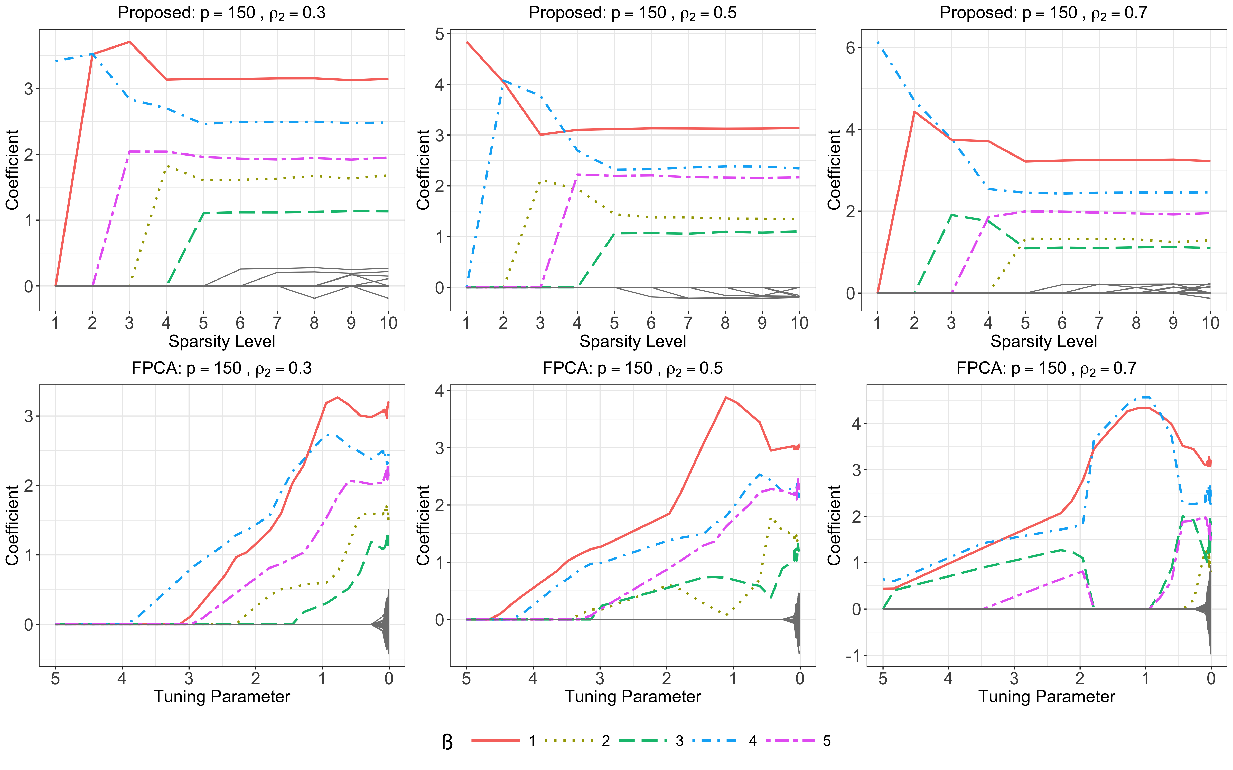
Figure 3: Solution paths of $\widehat{\beta}$ for different settings of for different $\rho_{2}$ corresponding to $(p,C_{0},\rho_{1})=(150,1,0.2)$. The colored lines correspond to the solution paths of the nonzero elements of $\beta$, whereas the grey ones correspond to zero elements.

Example 4.2.

In this example, we evaluate the Type I and II error rates of the proposed test statistic. Data settings are the same as in Example 4.1 except that $\xi(t)=\sum_{k=1}^{50}B(-1)^{k+1}k^{-2}\phi_{k}(t)$ with $B\in\{0,0.01,0.03,0.05,0.07,0.1\}$, which controls the signal strength. When $B=0$, we obtain the sizes. Because the testing results have similar patterns for different values of $(\rho_{1},\rho_{2})$, we report the sizes and powers when $(\rho_{1},\rho_{2})=(0.2,0.5)$ for the sake of a concise presentation. We choose $n\in\{200,400\}$, $p\in\{150,1500\}$ and the significance level to be 5%.

For the null hypothesis, $H_{0}:\xi(t)=0$, Table 3 summarizes the sizes and powers of the proposed test based on 1000 simulation runs. It reveals that the empirical sizes are reasonably controlled around the nominal level, and the empirical power increases with the sample size $n$ as well as the signal strength.

Table 3: Testing results of Monte Carlo averages with $\rho_{1}=0.2,\rho_{2}=0.5$.

$n$	$p$	$B=0$	$B=0.01$	$B=0.03$	$B=0.05$	$B=0.07$	$B=0.1$
200	150	0.057	0.111	0.112	0.817	0.969	1
	1500	0.053	0.117	0.117	0.784	0.955	0.999
400	150	0.055	0.137	0.137	0.982	0.999	1
	1500	0.057	0.115	0.115	0.978	0.999	1

5 ADNI Data Analysis

5.1 GIC Pathways

We denote model (1) in this subsection as Model 1. We treat the hippocampus morphometry surface as the two-dimensional function $Z_{i}(\cdot,\cdot)$. We also consider the following demographic covariates. Specifically, $X_{i}$ includes the allele codes of screened SNPs, the set of demographic covariates at baseline detailed in Section 2, and the top 5 principal components (PCs) of the whole genome data for correcting for population stratification (Price et al., 2006). Since the number of SNPs is significantly larger than the sample size, we first apply the sure independence screening approach (Fan and Lv, 2008) to reduce the number of candidate SNPs, while controlling the demographic variables and the top 5 PCs. We sort the SNPs in the decreasing order of their absolute correlations with each cognitive score and keep the top 1000 for each cognitive score. We combine the top 1000 SNPs of each score across all the 13 scores, leading to 10546 different SNPs in $X_{i}$. The $Y_{i}$ is one of the 13 cognitive scores at Month12 in Table S1, leading to 13 PFLMs. For easy comparison, we standardize all SNPs, cognitive scores and demographic variables, including Age and Years of education. As both left and right hippocampi have 2D radial radial distance measures and the two parts of hippocampi have been found to be asymmetric Pedraza et al. (2004), we apply our method to the left and right hippocampi separately. In the estimation procedure, the controlling variables are not penalized and are always in the active set. The initial value is set to be zero. We choose the sparsity level $J$ and the smoothness parameter $J$ by a grid search method with $J\in\{1,2,\dots,100\}$ and $\lambda$ from 50 evenly spaced points on $[1e-5,0.1]$.

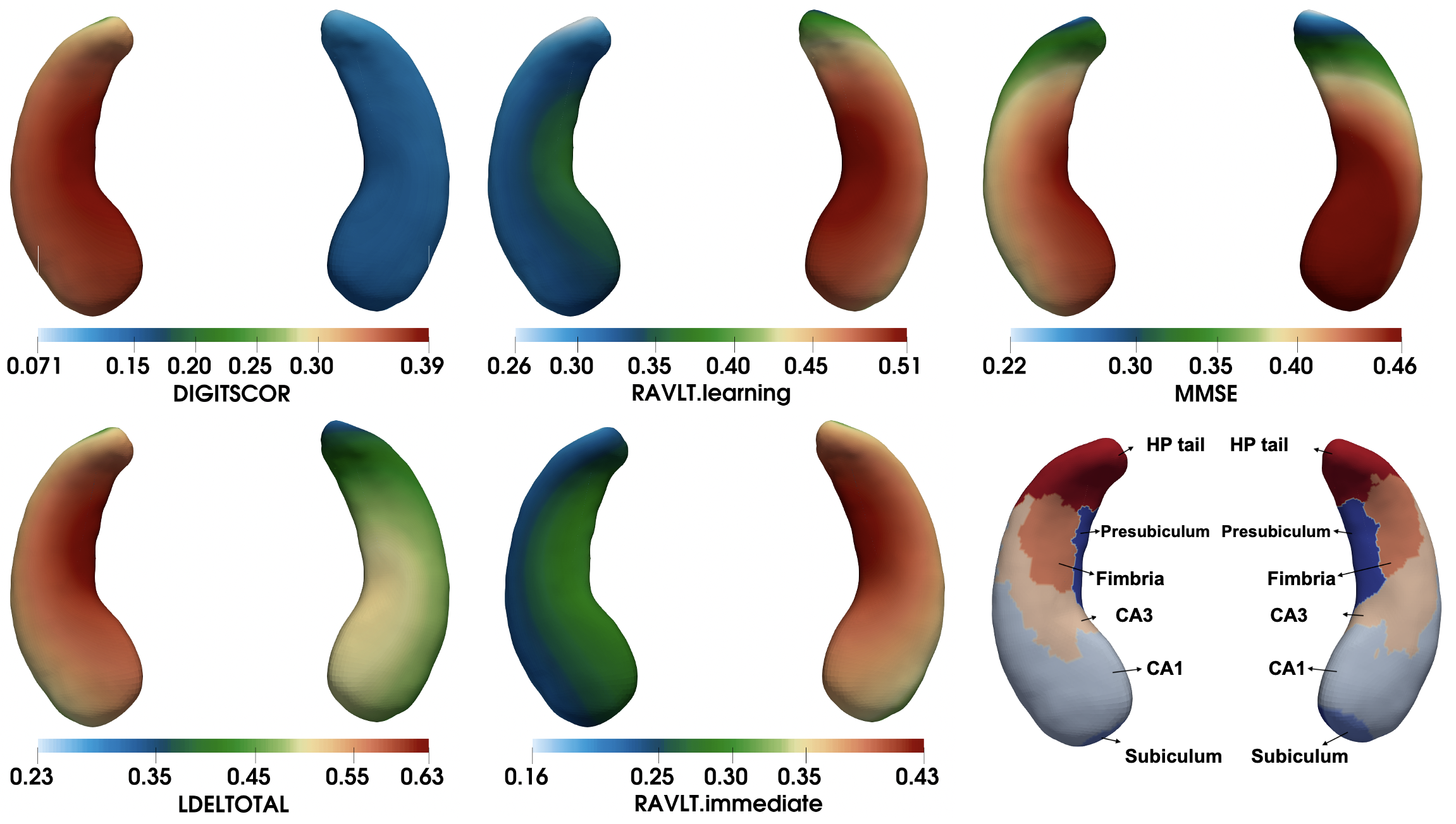
Figure 4: ADNI data analysis results: estimates of the left and right hippocampus surfaces for DIGITSCOR, LDELTOTAL, MMSE, RAVLT.immediate and RAVLT.learning for Model 1 and the hippocampal subfields (from left to right, and from top to bottom).

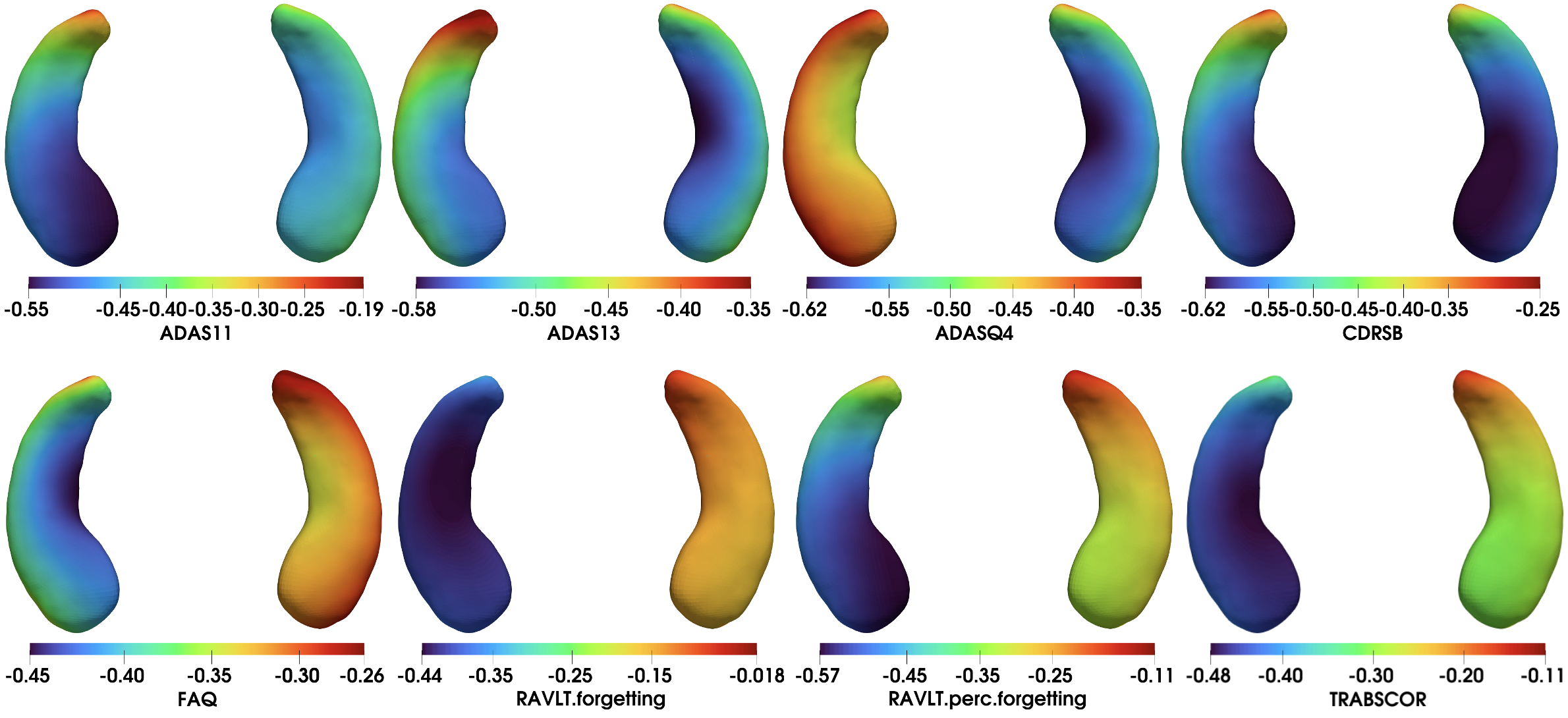
Figure 5: ADNI data analysis results: estimates of the the left and right hippocampus surfaces for ADAS11, ADAS13, ADASQ4, CDRSB, FAQ, RAVLT.forgetting, RAVLT.perc.forgetting and TRABSCOR for Model 1 (from left to right, and from top to bottom).

Figs 4 and 5, respectively, present the estimates of the left and right hippocampal surfaces for all the thirteen cognitive scores in Model 1. Fig 4 shows the estimates $\widehat{\xi}$, most of whose values range from 0.071 to 0.63, corresponding to DIGITSCOR, LDELTOTAL, MMSE, RAVLT.immediate, and RAVLT.learning. Fig 5 shows the estimates $\widehat{\xi}$, most of whose values range from -0.62 to -0.018, corresponding to ADAS11, ADAS13, ADASQ4, CDRSB, FAQ, RAVLT.forgetting, RAVLT.perc.forgetting, and TRABSCOR. Inspecting Figs 4 and 5 reveals the heterogeneous effects of the hippocampus on all the 13 cognitive scores. A bilateral and asymmetric hippocampal effect on the cognitive function is also observed. Among the six hippocampal subfields in Fig 4, CA1, presubiculum and subiculum show high sensitivity (Frisoni et al., 2008; De Flores et al., 2015). AD-related atrophy is initially focal in CA1 before spreading to other subfields.

Hereafter, we focus on the results using the left hippocampal surface data. Table 4 presents the estimates of selected important covariates and their corresponding raw $p$-fvalues for the 13 cognitive scores in Model 1. The $p$-values are obtained using the limit distribution in Theorem 3 of the supplementary material by taking the true value $\beta_{A^{*}}^{*}$ to be zero. Under the null hypothesis $H_{0}:\beta_{A^{*}}^{*}=0$, each element of $\widehat{\beta}_{A^{*}}$ converges to a normal distribution and we can use the corresponding null limit distribution to calculate the $p$-value. In consist with the existing literature (Vina and Lloret, 2010; Guerreiro and Bras, 2015; Zhang et al., 1990), age and education are significant for most of the cognitive scores. Generally, age produces a negative effect on the cognitive function. Education exhibits negative effects on scores with higher value indicating impairment as well as positive effects on scores with lower value indicating impairment. Retirement is significant for 6 scores, suggesting an excess risk of cognition deficit among retired individuals. Gender is significant for 5 scores and Handedness is significant for 3 scores.

Table 4: ADNI data analysis results: estimates with their corresponding raw $p$-values in parentheses of some selected covariates for the 13 cognitive scores.

Score	Model	Gender	Handedness	Education	Retirement	Age	APOE4	MCI	AD
ADAS11	Model 1	0.098(0.033)	0.110(0.204)	-0.078(0.001)	0.137(0.021)	0.051(0.028)	-	-	-
	Model 2	0.129(0.000)	0.145(0.012)	-0.091(0.000)	0.070(0.088)	0.074(0.000)	0.252(0.000)	-	-
	Model 3	0.136(0.000)	0.051(0.314)	-0.017(0.226)	-0.019(0.585)	0.062(0.000)	0.066(0.000)	0.823(0.000)	1.855(0.000)
ADAS13	Model 1	-0.034(0.333)	0.123(0.057)	-0.124(0.000)	0.007(0.872)	0.050 (0.005)	-	-	-
	Model 2	0.099(0.005)	0.084(0.207)	-0.176(0.000)	0.158(0.000)	0.040(0.023)	0.291(0.000)	-	-
	Model 3	0.164(0.000)	0.004(0.929)	0.028(0.021)	0.010(0.752)	0.043(0.001)	0.077(0.000)	0.994(0.000)	1.967(0.000)
ADASQ4	Model 1	-0.058(0.100)	0.161(0.016)	-0.138(0.000)	0.042(0.348)	-0.035(0.051)	-	-	-
	Model 2	-0.026(0.452)	0.135(0.037)	-0.169(0.000)	0.100(0.026)	0.007(0.698)	0.308(0.000)	-	-
	Model 3	0.007(0.757)	0.141(0.002)	-0.091(0.000)	-0.001(0.969)	0.006(0.612)	0.173(0.000)	1.118(0.000)	1.746(0.000)
CDRSB	Model 1	0.019(0.660)	0.097(0.220)	-0.091(0.000)	0.132(0.017)	0.047(0.027)	-	-	-
	Model 2	0.085(0.011)	-0.0.089(0.172)	-0.081(0.000)	0.265(0.004)	0.053(0.002)	0.215(0.000)	-	-
	Model 3	0.107(0.000)	-0.029(0.494)	0.016(0.154)	0.107(0.000)	0.046(0.000)	0.071(0.000)	0.819(0.000)	2.017(0.000)
FAQ	Model 1	0.050(0.232)	0.052(0.519)	-0.079(0.000)	0.278(0.000)	0.045(0.035)	-	-	-
	Model 2	0.145(0.004)	0.020(0.830)	-0.067(0.007)	0.273(0.000)	0.002(0.925)	0.238(0.000)	-	-
	Model 3	0.125(0.000)	0.038(0.429)	0.019(0.135)	0.128(0.000)	0.012(0.382)	0.118(0.000)	0.666(0.000)	1.952(0.000)
RAVLT.forgetting	Model 1	-0.026(0.580)	0.002(0.979)	-0.043(0.056)	-0.297(0.000)	-0.158(0.000)	-	-	-
	Model 2	-0.072(0.055)	-0.231(0.001)	-0.033(0.075)	-0.256(0.000)	-0.161(0.000)	0.148(0.000)	-	-
	Model 3	0.062(0.219)	-0.120(0.202)	0.002(0.953)	-0.173(0.008)	-0.047(0.064)	0.024(0.353)	0.637(0.000)	0.539(0.000)
RAVLT.perc.forgetting	Model 1	-0.106(0.005)	0.120(0.081)	-0.149(0.000)	-0.019(0.685)	-0.045(0.018)	-	-	-
	Model 2	-0.107(0.001)	0.295(0.000)	-0.125(0.000)	-0.009(0.830)	-0.047(0.003)	0.188(0.000)	-	-
	Model 3	-0.054(0.052)	0.022(0.659)	-0.054(0.000)	-0.170(0.000)	0.003(0.855)	0.093(0.000)	0.989(0.000)	1.481(0.000)
TRABSCOR	Model 1	-0.036(0.436)	-0.088(0.293)	-0.230(0.000)	-0.021(0.712)	0.003(0.876)	-	-	-
	Model 2	0.004(0.926)	-0.131(0.076)	-0.182(0.000)	0.023(0.065)	0.042(0.037)	0.180(0.000)	-	-
	Model 3	0.010(0.803)	-0.012(0.867)	-0.143(0.000)	0.000(1.000)	0.061(0.002)	0.052(0.011)	0.642(0.000)	1.484(0.000)
DIGITSCOR	Model 1	0.189(0.000)	0.038(0.584)	0.227(0.000)	0.151(0.002)	-0.076(0.000)	-	-	-
	Model 2	0.253(0.000)	-0.118(0.057)	0.192(0.000)	-0.051(0.230)	-0.088(0.000)	-0.176(0.000)	-	-
	Model 3	0.238(0.000)	-0.170(0.010)	0.130(0.000)	0.021(0.639)	-0.052(0.004)	-0.036(0.058)	-0.512(0.000)	-1.389(0.000)
LDELTOTAL	Model 1	0.077(0.067)	-0.209(0.009)	0.187(0.000)	-0.024(0.659)	-0.004(0.846)	-	-	-
	Model 2	0.293(0.000)	-0.159(0.006)	0.199(0.000)	0.100(0.010)	-0.035(0.025)	-0.349(0.000)	-	-
	Model 3	0.021(0.396)	-0.059(0.189)	0.105(0.000)	-0.052(0.090)	-0.034(0.007)	-0.135(0.000)	-1.329(0.000)	-1.868(0.000)
MMSE	Model 1	-0.043(0.215)	0.302(0.00)	0.071(0.000)	-0.121(0.008)	-0.049(0.006)	-	-	-
	Model 2	-0.006(0.847)	0.240(0.000)	0.141(0.000)	-0.161(0.000)	-0.008(0.609)	-0.230(0.000)	-	-
	Model 3	-0.159(0.000)	0.146(0.002)	0.019(0.130)	-0.080(0.011)	-0.038(0.003)	-0.103(0.000)	-0.670(0.000)	-1.752(0.000)
RAVLT.learning	Model 1	0.283(0.000)	-0.102(0.222)	0.123(0.000)	0.048(0.401)	-0.031(0.158)	-	-	-
	Model 2	0.268(0.000)	0.092(0.018)	0.124(0.000)	-0.002(0.972)	-0.047(0.010)	-0.227(0.000)	-	-
	Model 3	0.139(0.000)	0.122(0.047)	0.079(0.000)	-0.059(0.160)	0.018(0.296)	-0.045(0.009)	-0.910(0.000)	-1.240(0.000)
RAVLT.immediate	Model 1	0.425(0.000)	0.169(0.050)	0.228(0.000)	0.022(0.708)	-0.049(0.033)	-	-	-
	Model 2	0.457(0.000)	0.094(0.173)	0.227(0.000)	0.001 (0.980)	-0.039(0.034)	-0.268(0.000)	-	-
	Model 3	0.287(0.000)	-0.008(0.855)	0.147(0.000)	-0.134(0.000)	-0.008(0.531)	-0.106(0.000)	-0.973(0.000)	-1.602(0.000)

Model 1 corrects for all covariates except APOE4 and the baseline disease status; Model 2 corrects for all covariates except the baseline disease status; and Model 3 corrects for all covariates.

Fig 6 and Fig 6 present the ideogram and Manhattan plots of significant SNPs for all the 13 scores in Model 1, respectively. Inspecting Fig 6 reveals heterogeneous genetic effects across all the scores, but several well-known SNPs on the 19th chromosome are identified to be important for all the 13 cognitive scores. Table 5 lists SNPs on the 19th chromosome identified to be important for at least 3 cognitive scores. The rs429358 on the 19th chromosome, which is one of the two variants for the well-known APOE alleles, is significant for ADAS11, ADAS13, FAQ, MMSE, RAVLT.immediate, RAVLT.perc.forgetting. Other SNPs include rs283812, in the PVRL2 region, rs769449 in the APOE region, rs66626994 in the APOC1 region. The APOE, PVRL2 and APOC1 regions in the cytogenetic region 19q13.32 are high AD-risk regions (Carrasquillo et al., 2009; Vermunt et al., 2019).

Except for the 19th chromosome, two SNPs are also identified to be important for at least 3 scores, including rs28414114 from chromosome 14 with the smallest $p$-value 7e-14 and rs12108758 from chromosome 5 with the smallest $p$-value 2e-9. Furthermore, we obtain the $p$-values of the selected SNPs in Fig 6. The $p$-values of several important SNP are smaller than $0.05/10145$ (10145 SNPs after screening).

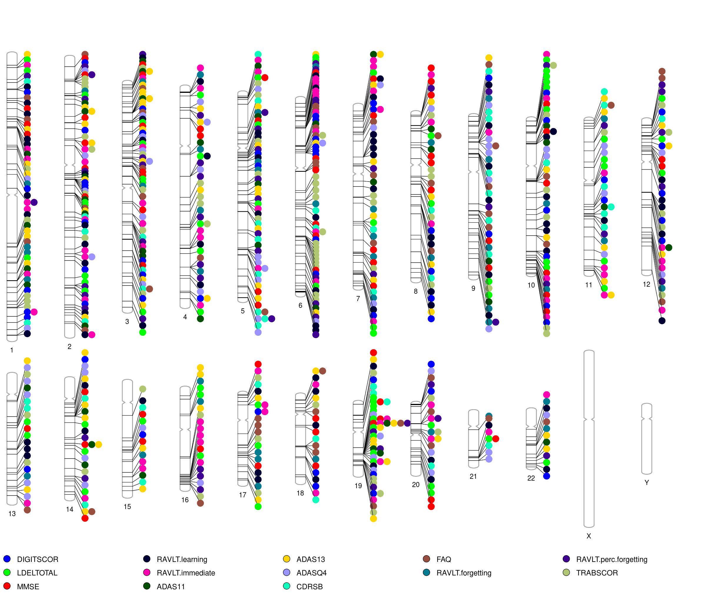
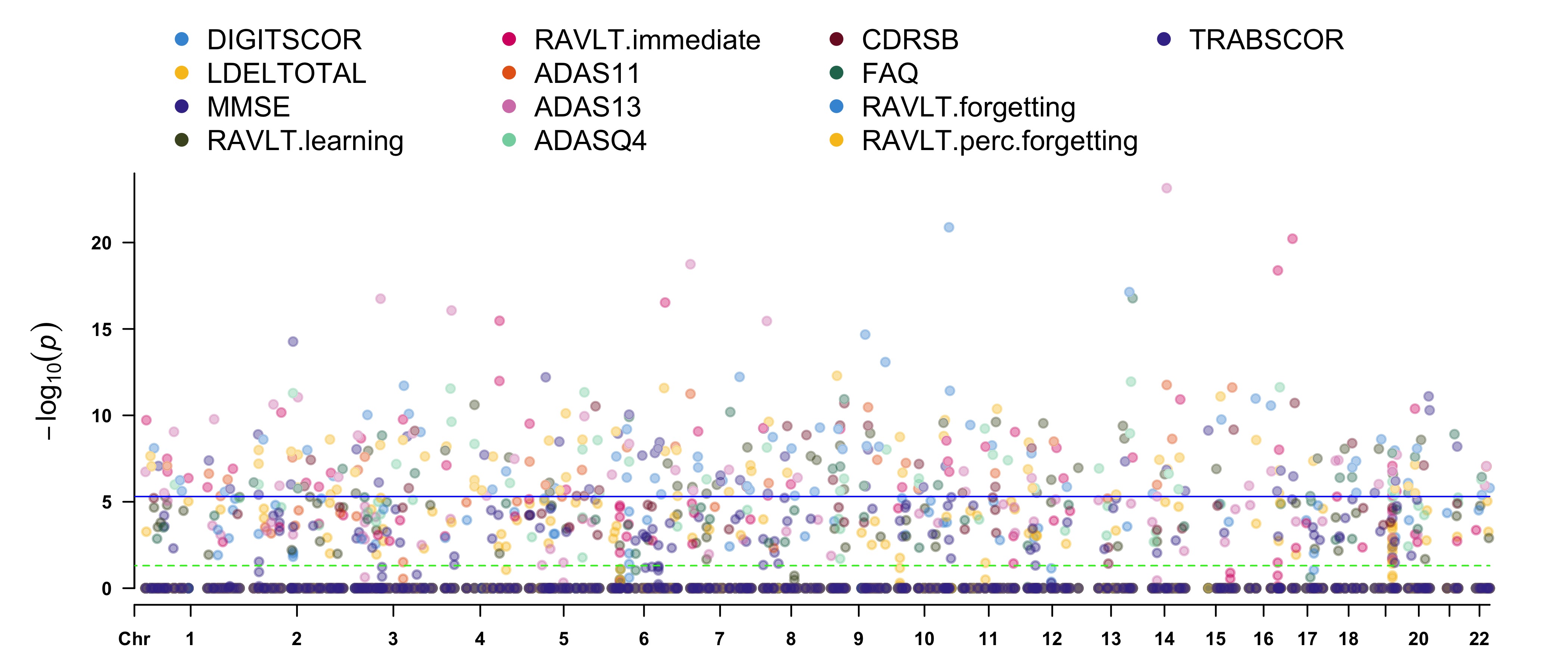
Figure 6: Panel (a) presents positions of the important SNPs for the 13 scores for Models 1. The colors represent the 13 scores and each signal dot indicates the SNP is selected for the corresponding score. Panel (b) gives $p$-values of the selected SNPs for Model 1. The blue line indicates the threshold $p$-value$=0.05/10154$.

Table 5: Detailed information of the common SNPs from the 19th chromosome for at least 3 scores for Model 1.

SNP	Chr	Base Pair	Scores
rs283812	19	45388568	CDRSB, LDELTOTAL, MMSE
rs769449	19	45410002	LDELTOTAL, MMSE, RAVLT.immediate
rs429358	19	45411941	ADAS11, ADAS13, FAQ, MMSE, RAVLT.immediate, RAVLT.perc.forgetting
rs66626994	19	45428234	ADAS13, LDELTOTAL, RAVLT.immediate

5.2 Conditional GIC (CGIC) pathways given APOE4

We denote model (1) in this subsection as Model 2. Model 2 is almost the same as Model 1 except that we exclude the SNPs in the 19q13.32 region from the candidate SNPs and include the number of APOE4 gene copies as one of the controlling covariates. In our dataset, 230 subjects had one APOE4 allele and 67 subjects had two APOE4 alleles. The cytogenetic region 19q13.32 contains 6376 SNPs in this region, including the well-known APOE (Bertram and Tanzi, 2012; Zhao et al., 2021). It allows us to better understand the conditional effects of other SNPs on cognitive scores given on the APOE4 alleles. We apply the same screening step and Algorithm 1 to Model 2 for each cognitive score.

Table 4 presents the related estimation results corresponding to Model 2. Estimates of the demographic covariates in Model 2 are similar to their corresponding estimates in Model 1. The number of APOE4 alleles is significant for all the scores, while exhibiting negative effects on cognitive ability. Estimates of the hippocampal surface for the 13 scores in Model 2 are similar to those in Model 1, so we include them in the supplementary material.

Fig S5(a) of the supplementary material presents the ideogram of the selected important SNPs for Model 2. For each cognitive score, the selected significant SNPs in Model 2 enjoy some similarities with those in Model 1. For instance, rs28414114 from chromosome 14 are also identified to be important for ADAS11 and ADAS13. Meanwhile, regions of the selected SNPs for some scores are similar to that in Model 1. For example, positions of the important SNPs for TABSCOR in chromosome 6 are from 81858848 to 91078328 with the smallest $p$-value 9.06e-11 and from 120546293 to 120765041 with the smallest $p$-value 8e-9 in Model 1, and in Model 2 the important positions are from 80949537 to 94053838 with the smallest $p$-value 1.16e-9 and from 120533534 to 120771669 with the smallest $p$-value 6e-15.

5.3 CGIC pathways given APOE4 and disease status

We denote model (1) in this subsection as Model 3. Model 3 is almost the same as Model 2 except that we further include the baseline diagnosis status as one of the controlling covariates. The baseline diagnosis status is coded by using two dummy variables: MCI and AD. Because clinical notes provide supplementary information and are considered on a case-by-case basis, the effects of the SNPs on change in cognitive performance may be confounded with the effects of differences in baseline diagnosis. We are interested in whether the relationships would alter when adjusting for the baseline diagnosis status. We apply the same screening step and Algorithm 1 to Model 3 for each cognitive score.

Table 4 also presents the related estimation results corresponding to Model 3. After introducing the baseline diagnosis status, almost all estimates of the demographic covariates and APOE4 in Model 3 are smaller than their corresponding estimates in Models 1 and 2. The baseline status MCI has significant positive effects on ADAS11, ADAS13, CDRSB, FAQ, RAVLT.forgetting, RAVLT.perc.forgetting and TRABSCOR, and exhibit significant negative effects on DIGITSCOR, LDELTOTAL, MMSE, RAVLT.learning and RAVLT.immediate. The baseline status AD generally has stronger effects on the 13 scores in Month 12 than the baseline MCI status. Similar patterns of the hippocampal estimates are also observed for the 13 scores to those in Section 5.1 and we include the corresponding results in the supplementary material.

Fig S5(b) of the supplementary material presents the ideogram of the selected important SNPs for Model 3. The selected important SNPs seem quite different to the SNPs in Fig 6. This is reasonable because we consider the baseline diagnosis status in the screening step and always keep it in the model. The selected important SNPs for at least 3 scores are rs13101604 from chromosome 4 with the smallest $p$-value 4.18e-9, rs2442696 from chromosome 4 with the smallest $p$-value 6.96e-11, and rs4761161 from chromosome 12 with the smallest $p$-value 2.11e-09.

5.4 Comparisons of the three models

In this subsection, we compare the above three models in terms of the shared and different heritability patterns of the 13 scores and the proportions of the variations explained in cognitive deficits by the three types of data: the genetic data, the controlling covariates and the hippocampal surface data. The average computation times of the proposed method are 2.25 hours with the standard error 0.41 hour for Model 1, 2.31 hours with the standard error 0.44 hour for Model 2, and 2.19 hours with the standard error 0.45 hour for Model 3.

Although most human traits have a polygenic architecture (Wray et al., 2018), heritability can be used to measure how much of the variation in each score is due to variation in genetic data (Yang et al., 2010). By definition, we estimate the heritability for the three models by calculating the phenotypic variance due to the genetic variables. We estimate the phenotypic variance by the empirical variance of $X_{iG}^{\top}\hat{\beta}_{G}$, where $X_{iG}$ is the genetic variables of the $i$-th subject and $\hat{\beta}_{G}$ is the corresponding coefficient estimates. For Model 2 and Model 3, estimates of the heritability are based on the considered SNPs which excludes the SNPs in the cytogenetic region 19q13.32. Fig 7 gives the heritability estimates of the genetic effects for the cognitive scores. Heritability of the cognitive scores are estimated to be 62.69%$\sim$78.01% for Model 1, and 55.56%$\sim$85.62% for Model 2, and 33.02%$\sim$69.66% for Model 3. The remaining heritability of the scores, especially RAVLT.forgetting, is still relatively high even after accounting for APOE4. It is consistent with previous research and suggests that memory functioning in AD is under strong genetic influence that is only partly attributable to APOE genotype (Wilson et al., 2011). However, there are 1.1%$\sim$35.3% decreases of the heritability estimates of the 13 scores for Model 3. It reveals that the baseline diagnosis status explains a part of the cognitive function associated to the polygenic effect.

We also examine the effect size of the controlling covariates by calculating the proportion of variance explained by these covariates in Fig 7. The proportions of variance explained by the controlling variables increase with the inclusion of the number of APOE4 alleles and the baseline disease status.

Fig 7 presents the effect size of the imaging covariates. The hippocampal surface data account for 1% $\sim$4.6% of the total variantions in 13 cognitive scores for Model 1, 0.1%$\sim$4.1% for Model 2 and 0.005%$\sim$0.63% for Model 3. These results suggest that the baseline diagnosis status explains a larger part of the cognitive function associated to the hippocampal data compared to the number of APOE4 gene alleles. We also compare the effects of the genetic data with that of the imaging data. The above results show that the cognitive function may have the polygeneic inheritance, which is not controlled by one gene, but by multiple genes that each make a small contribution to the overall outcome. There are 75 genes on average selected to be important for the congnitive scores in the three models. The variance explained by a single gene is about 0.84%$\sim$1.05%, 0.74% $\sim$ 1.14% and 0.44% $\sim$ 0.93% in the three models, which is comparable to that of the imaging data. Furthermore, we calculate the estimated $p$-values of left and right hippocampal surface data for the 13 cognitive scores in the three models in Table 6. The left hippocampus is significant at 5% significance level for 9 scores, 11 scores and 5 scores in Model1, Model 2 and Model 3, respectively. The right one is significant for 7 scores, 11 scores, and 3 scores in Model1, Model 2 and Model 3, respectively. Both the left and right hippocampa are significant for ADAS13 and MMSE, which are consistent with the findings in Morrison et al. (2022) and Peng et al. (2015). It can also be observed that most of the $p$-values in Model 3 are larger than the corresponding $p$-values in Model 1 and Model 2.

Table 6: Estimated $p$-values of hippocampal surface data for the 13 cignitive scores.

	Model 1			Model 2			Model 3
Score	Left	Right		Left	Right		Left	Right
ADAS11	3.66E-05	1.35E-08		6.72E-05	1.04E-05		0.054	0.046
ADAS13	1.58E-08	1.49E-09		6.36E-08	2.11E-05		0.016	0.023
ADASQ4	2.55E-07	2.82E-05		3.41E-07	2.88E-06		0.052	0.096
CDRSB	4.56E-07	4.27E-06		2.25E-05	0.008		0.105	0.142
FAQ	3.72E-05	0.753		0.998	0.003		0.039	0.102
RAVLT.forgetting	0.707	0.999		0.160	0.257		0.999	0.120
RAVLT.perc.forgetting	0.001	0.824		9.89E-05	2E-04		0.132	0.071
TRABSCOR	0.916	0.999		0.007	0.001		0.011	0.090
DIGITSCOR	0.036	0.999		0.001	0.381		0.117	0.582
LDELTOTAL	2.19E-07	1.82E-09		0.001	7.22E-06		0.032	0.160
MMSE	2.66E-10	5.35E-11		0.002	1.06E-05		0.022	0.039
RAVLT.learning	0.998	7.80E-05		2E-04	5.70E-05		0.999	0.080
RAVLT.immediate	0.999	0.999		7.83E-05	4E-04		0.161	0.329

Model 1 corrects for all covariates except APOE4 and the baseline disease status; Model 2 corrects for all covariates except the baseline disease status; and Model 3 corrects for all covariates.

Genetic correlation has been proposed to describe the shared genetic associations within pairs of quantitative traits, and it can be calculated as the correlation of the genetic effects of numerous SNPs on the traits (Zhao and Zhu, 2022). To provide critical information about the fundamental biological pathways and describe the shared genetic etiology of the 13 scores, we calculate the genetic correlations between the 13 scores for the 3 models that we have considered in Figs 7-7. There exist strong genetic correlations between the 13 scores for Model 1, which suggest the overall similarity of the genetic architecture on brain functions in Month 12 characterizing by these scores. The genetic correlations adjusting for the number of APOE4 alleles are similar to that for Model 1 with slightly smaller values, indicating the shared genetic effects for the 13 scores besides the effect of the well known APOE4 gene. However, the genetic correlations decrease a lot when additionally controlling for the baseline diagnosis status, which is supposed to explain a large part of the shared genetic effect on the cognitive scores. Also, it reveals that greater genetic heterogeneity exists after accounting for the baseline diagnosis status. One potential reason is that the population of AD is genetically heterogeneous (Lo et al., 2019). Adjusting for disease status suggests that within a given diagnostic group, there is substantial variation in cognitive scores that is explained by genetic markers, suggesting heterogeneity within disease classifications that is partially explained by genetics. It may indicate that different therapies are needed for different symptoms after the AD onset.

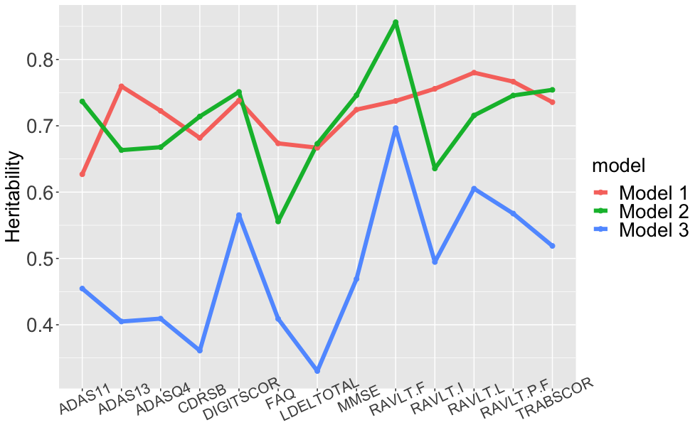
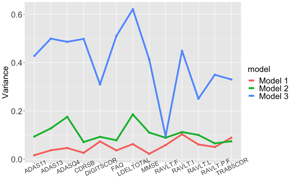
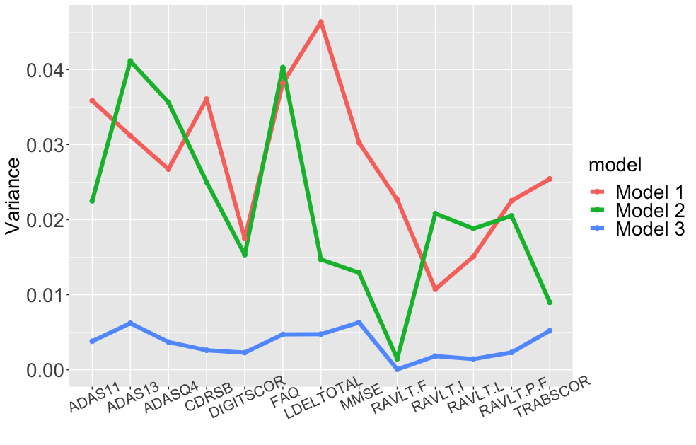
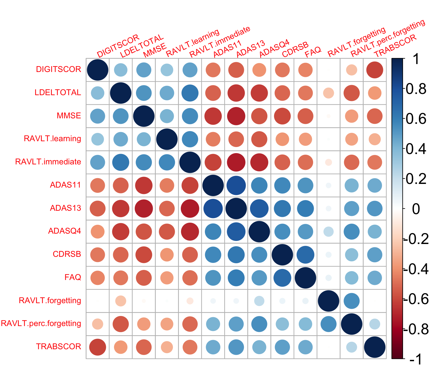
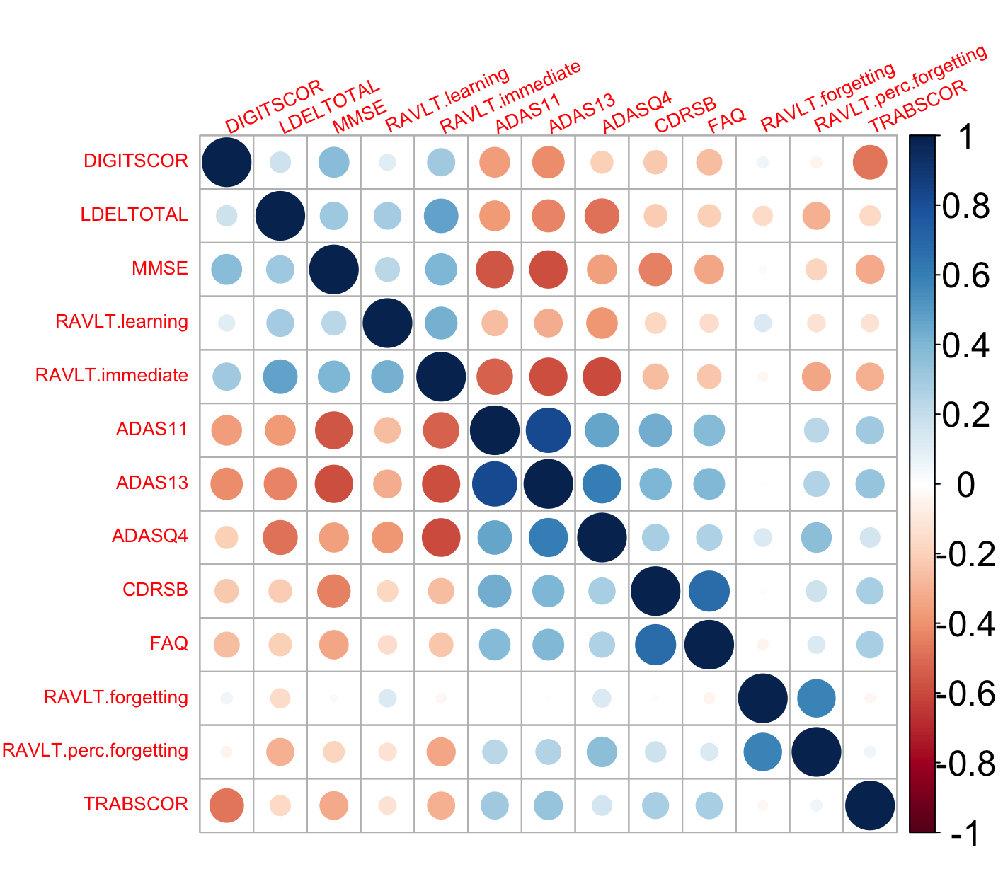
Figure 7: Heritability estimates of the genetic data (a) and the proportions of variance explained by the controlling variables (b) and the imaging data (c). Genetic correlations between the 13 cognitive scores for Model 1 (d), Model 2 (e) and Model 3 (f). The red line indicates Model 1, the green line indicates Model 2 and the blue line indicates Model 3.

6 Discussion

This paper aims at mapping the biological pathways of phenotypes of interest from the ADNI study by integrating GIC data. The high dimensional genetic data and the features of the hippocampal surface data motivate us to consider a high-dimensional PFLM to establish the associations between the genetic and imaging data with the phenotype of interest. We proposed a new estimation method to high-dimensional PFLMs under the RKHS framework and the $\ell_{0}$ penalty, and investigated the theoretical results of the estimators. Through the analyses of the ADNI study, we have shown that the proposed method is a valuable statistical tool for quantifying the complex relationships between phenotypes of interest and the GIC data.

Although the proposed method considers one functional covariate, it can be extended to accommodate multiple functional covariates. We can consider the following high-dimensional PFLM with multiple functional predictors,

$$Y_{i}=\alpha+X_{i}^{\top}\beta+\sum_{k=1}^{K}\int_{\mathcal{T}}Z_{ik}(t)\xi_{k}(t)dt+\epsilon_{i}.$$

Each $\xi_{k}(t)$ is assumed to be in a reproducing kernel Hilbert space. Similar to the minimization problem in (2) that imposes $\ell_{0}$ penalty to $\beta$ and RKHS roughness penalty on $\xi(t)$, we can estimate $\{\xi_{k}(t)\}$s by imposing RKHS roughness penalty on each $\xi_{k}(t)$. The representer theorem and the theoretical results can be obtained similarly. Such extensions are worthy of further investigation.

References

- (1) Battista, P., C. Salvatore, and I. Castiglioni. Optimizing neuropsychological assessments for cognitive, behavioral, and functional impairment classification: a machine learning study. Behavioural neurology 2017, 1–19.
- Bertram and Tanzi (2012) Bertram, L. and R. E. Tanzi (2012). The genetics of alzheimer’s disease. Progress in molecular biology and translational science 107, 79–100.
- Blokland et al. (2012) Blokland, G. A., G. I. de Zubicaray, K. L. McMahon, and M. J. Wright (2012). Genetic and environmental influences on neuroimaging phenotypes: a meta-analytical perspective on twin imaging studies. Twin Research and Human Genetics 15(3), 351–371.
- Braak and Braak (1998) Braak, H. and E. Braak (1998). Evolution of neuronal changes in the course of Alzheimer’s disease. Springer.
- Cai and Yuan (2011) Cai, T. T. and M. Yuan (2011). Optimal estimation of the mean function based on discretely sampled functional data: Phase transition. The Annals of Statistics 39(5), 2330–2355.
- Cai and Yuan (2012) Cai, T. T. and M. Yuan (2012). Minimax and adaptive prediction for functional linear regression. Journal of the American Statistical Association 107(499), 1201–1216.
- Carrasquillo et al. (2009) Carrasquillo, M. M., F. Zou, V. S. Pankratz, S. L. Wilcox, L. Ma, L. P. Walker, S. G. Younkin, C. S. Younkin, L. H. Younkin, G. D. Bisceglio, et al. (2009). Genetic variation in pcdh11x is associated with susceptibility to late-onset alzheimer’s disease. Nature genetics 41(2), 192–198.
- Cruciani et al. (2022) Cruciani, F., A. Altmann, M. Lorenzi, G. Menegaz, and I. B. Galazzo (2022). What pls can still do for imaging genetics in alzheimer’s disease. In 2022 IEEE-EMBS International Conference on Biomedical and Health Informatics (BHI), pp. 1–4. IEEE.
- de Aquino (2021) de Aquino, C. H. (2021). Methodological issues in randomized clinical trials for prodromal alzheimer’s and parkinson’s disease. Frontiers in Neurology 12.
- De Flores et al. (2015) De Flores, R., R. La Joie, and G. Chételat (2015). Structural imaging of hippocampal subfields in healthy aging and alzheimer’s disease. Neuroscience 309, 29–50.
- Deary et al. (2022) Deary, I. J., S. R. Cox, and W. D. Hill (2022). Genetic variation, brain, and intelligence differences. Molecular Psychiatry 27, 335–353.
- Dukart et al. (2016) Dukart, J., F. Sambataro, and A. Bertolino (2016). Accurate prediction of conversion to alzheimer’s disease using imaging, genetic, and neuropsychological biomarkers. Journal of Alzheimer’s Disease 49(4), 1143–1159.
- Duong et al. (2022) Duong, M. T., S. R. Das, X. Lyu, L. Xie, H. Richardson, S. X. Xie, P. A. Yushkevich, D. A. Wolk, and I. M. Nasrallah (2022). Dissociation of tau pathology and neuronal hypometabolism within the atn framework of alzheimer’s disease. Nature communications 13(1), 1–15.
- Elliott et al. (2018) Elliott, L. T., K. Sharp, F. Alfaro-Almagro, S. Shi, K. L. Miller, G. Douaud, J. Marchini, and S. M. Smith (2018). Genome-wide association studies of brain imaging phenotypes in UK Biobank. Nature 562(7726), 210–216.
- Fan and Li (2001) Fan, J. and R. Li (2001). Variable selection via nonconcave penalized likelihood and its oracle properties. Journal of the American statistical Association 96(456), 1348–1360.
- Fan and Lv (2008) Fan, J. and J. Lv (2008). Sure independence screening for ultra-high dimensional feature space. Journal of the Royal Statistical Society: Series B (Statistical Methodology) 70(5), 849–911.
- Frisoni et al. (2008) Frisoni, G. B., R. Ganzola, E. Canu, U. Rüb, F. B. Pizzini, F. Alessandrini, G. Zoccatelli, A. Beltramello, C. Caltagirone, and P. M. Thompson (2008). Mapping local hippocampal changes in alzheimer’s disease and normal ageing with mri at 3 tesla. Brain 131(12), 3266–3276.
- Grassi et al. (2019) Grassi, M., N. Rouleaux, D. Caldirola, D. Loewenstein, K. Schruers, G. Perna, M. Dumontier, and A. D. N. Initiative (2019). A novel ensemble-based machine learning algorithm to predict the conversion from mild cognitive impairment to alzheimer’s disease using socio-demographic characteristics, clinical information, and neuropsychological measures. Frontiers in neurology, 756.
- Guerreiro and Bras (2015) Guerreiro, R. and J. Bras (2015). The age factor in alzheimer’s disease. Genome medicine 7(1), 1–3.
- Hobart et al. (2013) Hobart, J., S. Cano, H. Posner, O. Selnes, Y. Stern, R. Thomas, J. Zajicek, and A. D. N. Initiative (2013). Putting the alzheimer’s cognitive test to the test i: traditional psychometric methods. Alzheimer’s & Dementia 9(1), S4–S9.
- Huang et al. (2018) Huang, J., Y. Jiao, Y. Liu, and X. Lu (2018). A constructive approach to l0 penalized regression. The Journal of Machine Learning Research 19(1), 403–439.
- Knutson et al. (2020) Knutson, K. A., Y. Deng, and W. Pan (2020). Implicating causal brain imaging endophenotypes in alzheimer’s disease using multivariable iwas and GWAS summary data. NeuroImage 223, 117347.
- Kong et al. (2016) Kong, D., K. Xue, F. Yao, and H. H. Zhang (2016). Partially functional linear regression in high dimensions. Biometrika 103(1), 147–159.
- Li and Zhang (2021) Li, C. and H. Zhang (2021). Tensor quantile regression with application to association between neuroimages and human intelligence. The Annals of Applied Statistics 15(3), 1455–1477.
- Li et al. (2007) Li, S., F. Shi, F. Pu, X. Li, T. Jiang, S. Xie, and Y. Wang (2007). Hippocampal shape analysis of alzheimer disease based on machine learning methods. American Journal of Neuroradiology 28(7), 1339–1345.
- Li and Zhu (2020) Li, T. and Z. Zhu (2020). Inference for generalized partial functional linear regression. Statistica Sinica 30, 1379–1397.
- Lindquist (2008) Lindquist, M. A. (2008). The statistical analysis of fmri data.
- Lo et al. (2019) Lo, M.-T., K. Kauppi, C.-C. Fan, N. Sanyal, E. T. Reas, V. Sundar, W.-C. Lee, R. S. Desikan, L. K. McEvoy, C.-H. Chen, and A. D. G. Consortium (2019). Identification of genetic heterogeneity of alzheimer’s disease across age. Neurobiology of aging 84, 243.e1–243.e9.
- Ma et al. (2019) Ma, H., T. Li, H. Zhu, and Z. Zhu (2019). Quantile regression for functional partially linear model in ultra-high dimensions. Computational Statistics & Data Analysis 129, 135–147.
- McKhann et al. (2011) McKhann, G. M., D. S. Knopman, H. Chertkow, B. T. Hyman, C. R. Jack Jr, C. H. Kawas, W. E. Klunk, W. J. Koroshetz, J. J. Manly, R. Mayeux, et al. (2011). The diagnosis of dementia due to alzheimer’s disease: Recommendations from the national institute on aging-alzheimer’s association workgroups on diagnostic guidelines for alzheimer’s disease. Alzheimer’s & dementia 7(3), 263–269.
- Morrison et al. (2022) Morrison, C., M. Dadar, N. Shafiee, S. Villeneuve, D. L. Collins, A. D. N. Initiative, et al. (2022). Regional brain atrophy and cognitive decline depend on definition of subjective cognitive decline. NeuroImage: Clinical 33, 102923.
- Ossenkoppele et al. (2021) Ossenkoppele, R., A. Leuzy, H. Cho, C. H. Sudre, O. Strandberg, R. Smith, S. Palmqvist, N. Mattsson-Carlgren, T. Olsson, J. Jögi, et al. (2021). The impact of demographic, clinical, genetic, and imaging variables on tau pet status. European journal of nuclear medicine and molecular imaging 48, 2245–2258.
- Pedraza et al. (2004) Pedraza, O., D. Bowers, and R. Gilmore (2004). Asymmetry of the hippocampus and amygdala in mri volumetric measurements of normal adults. Journal of the International Neuropsychological Society 10(5), 664–678.
- Peng et al. (2015) Peng, G.-P., Z. Feng, F.-P. He, Z.-Q. Chen, X.-Y. Liu, P. Liu, and B.-Y. Luo (2015). Correlation of hippocampal volume and cognitive performances in patients with either mild cognitive impairment or alzheimer’s disease. CNS neuroscience & therapeutics 21(1), 15–22.
- Price et al. (2006) Price, A. L., N. J. Patterson, R. M. Plenge, M. E. Weinblatt, N. A. Shadick, and D. Reich (2006). Principal components analysis corrects for stratification in genome-wide association studies. Nature genetics 38(8), 904–909.
- Ramsay and Silverman (2005) Ramsay, J. O. and B. W. Silverman (2005). Functional Data Analysis (2nd edition). Springer.
- Reiss and Ogden (2010) Reiss, P. T. and R. T. Ogden (2010). Functional generalized linear models with images as predictors. Biometrics 66(1), 61–69.
- Selkoe and Hardy (2016) Selkoe, D. J. and J. Hardy (2016). The amyloid hypothesis of alzheimer’s disease at 25 years. EMBO molecular medicine 8(6), 595–608.
- Shen and Thompson (2019) Shen, L. and P. M. Thompson (2019). Brain imaging genomics: integrated analysis and machine learning. Proceedings of the IEEE 108(1), 125–162.
- Sudlow et al. (2015) Sudlow, C., J. Gallacher, N. Allen, V. Beral, P. Burton, J. Danesh, P. Downey, P. Elliott, J. Green, M. Landray, et al. (2015). Uk biobank: an open access resource for identifying the causes of a wide range of complex diseases of middle and old age. PLoS Medicine 12(3), e1001779.
- Vermunt et al. (2019) Vermunt, L., S. A. Sikkes, A. Van Den Hout, R. Handels, I. Bos, W. M. Van Der Flier, S. Kern, P.-J. Ousset, P. Maruff, I. Skoog, et al. (2019). Duration of preclinical, prodromal, and dementia stages of alzheimer’s disease in relation to age, sex, and apoe genotype. Alzheimer’s & Dementia 15(7), 888–898.
- Vina and Lloret (2010) Vina, J. and A. Lloret (2010). Why women have more alzheimer’s disease than men: gender and mitochondrial toxicity of amyloid- peptide. Journal of Alzheimer’s disease 20(s2), S527–S533.
- Wang et al. (2016) Wang, J.-L., J.-M. Chiou, and H.-G. Müller (2016). Functional data analysis. Annual Review of Statistics and Its Application 3, 257–295.
- Wang et al. (2013) Wang, L., Y. Kim, and R. Li (2013). Calibrating non-convex penalized regression in ultra-high dimension. The Annals of statistics 41(5), 2505–2536.
- Wang et al. (2017) Wang, X., H. Zhu, and A. D. N. Initiative (2017). Generalized scalar-on-image regression models via total variation. Journal of the American Statistical Association 112(519), 1156–1168.
- Wilson et al. (2011) Wilson, R. S., S. Barral, J. H. Lee, S. E. Leurgans, T. M. Foroud, R. A. Sweet, N. Graff-Radford, T. D. Bird, R. Mayeux, and D. A. Bennett (2011). Heritability of different forms of memory in the late onset alzheimer’s disease family study. Journal of Alzheimer’s Disease 23(2), 249–255.
- Wray et al. (2018) Wray, N. R., C. Wijmenga, P. F. Sullivan, J. Yang, and P. M. Visscher (2018). Common disease is more complex than implied by the core gene omnigenic model. Cell 173(7), 1573–1580.
- Yang et al. (2010) Yang, J., B. Benyamin, B. P. McEvoy, S. Gordon, A. K. Henders, D. R. Nyholt, P. A. Madden, A. C. Heath, N. G. Martin, G. W. Montgomery, M. E. Goddard, and P. M. Visscher (2010). Common snps explain a large proportion of the heritability for human height. Nature genetics 42(7), 565–569.
- Yao et al. (2017) Yao, F., S. Sue-Chee, and F. Wang (2017). Regularized partially functional quantile regression. Journal of Multivariate Analysis 156, 39–56.
- Yuan and Cai (2010) Yuan, M. and T. T. Cai (2010). A reproducing kernel Hilbert space approach to functional linear regression. The Annals of Statistics 38(6), 3412–3444.
- Zhang et al. (1990) Zhang, M., R. Katzman, D. Salmon, H. Jin, G. Cai, Z. Wang, G. Qu, I. Grant, E. Yu, P. Levy, et al. (1990). The prevalence of dementia and alzheimer’s disease in shanghai, china: impact of age, gender, and education. Annals of Neurology: Official Journal of the American Neurological Association and the Child Neurology Society 27(4), 428–437.
- Zhao et al. (2019) Zhao, B., J. G. Ibrahim, Y. Li, T. Li, Y. Wang, Y. Shan, Z. Zhu, F. Zhou, J. Zhang, C. Huang, et al. (2019). Heritability of regional brain volumes in large-scale neuroimaging and genetic studies. Cerebral Cortex 29(7), 2904–2914.
- Zhao et al. (2021) Zhao, B., T. Li, S. M. Smith, D. Xiong, Y. Yang, X. Wang, T. Luo, Z. Zhu, Y. Shan, Z. Wu, et al. (2021). Genetic influences on the intrinsic and extrinsic functional organizations of the cerebral cortex. medRxiv.
- Zhao et al. (2019) Zhao, B., T. Luo, T. Li, Y. Li, J. Zhang, Y. Shan, X. Wang, L. Yang, F. Zhou, Z. Zhu, and H. Zhu (2019). GWAS of 19,629 individuals identifies novel genetic variants for regional brain volumes and refines their genetic co-architecture with cognitive and mental health traits. Nature Genetics 51, 1637–1644.
- Zhao and Zhu (2022) Zhao, B. and H. Zhu (2022). On genetic correlation estimation with summary statistics from genome-wide association studies. Journal of the American Statistical Association 117(537), 1–11.
- Zhao et al. (2019) Zhao, H., Q. Wu, G. Li, and J. Sun (2019). Simultaneous estimation and variable selection for interval-censored data with broken adaptive ridge regression. Journal of the American Statistical Association.
- Zhou et al. (2013) Zhou, H., L. Li, and H. Zhu (2013). Tensor regression with applications in neuroimaging data analysis. Journal of the American Statistical Association 108(502), 540–552.
- Zhou et al. (2014) Zhou, I. Y., Y.-X. Liang, R. W. Chan, P. P. Gao, J. S. Cheng, Y. Hu, K.-F. So, and E. X. Wu (2014). Brain resting-state functional mri connectivity: morphological foundation and plasticity. Neuroimage 84, 1–10.
- Zhu et al. (2022) Zhu, H., T. Li, and B. Zhao (2022). Statistical learning methods for neuroimaging data analysis with applications. arXiv preprint arXiv:2210.09217.