Slow semiclassical dynamics of a two-dimensional Hubbard model
in disorder-free potentials

Abstract

The quench dynamics of the Hubbard model in tilted and harmonic potentials is discussed within the semiclassical picture. Applying the fermionic truncated Wigner approximation (fTWA), the dynamics of imbalances for charge and spin degrees of freedom is analyzed and its time evolution is compared with the exact simulations in one-dimensional lattice. Quench from charge or spin density wave is considered. We show that introduction of harmonic and spin-dependent linear potentials sufficiently validates fTWA for longer times. Such an improvement of fTWA is also obtained for the higher order correlations in terms of quantum Fisher information for charge and spin channels. This allows us to discuss the dynamics of larger system sizes and connect our discussion to the recently introduced Stark many-body localization. In particular, we focus on a finite two-dimensional system and show that at intermediate linear potential strength, the addition of a harmonic potential and spin dependence of the tilt, results in subdiffusive dynamics, similar to that of disordered systems. Moreover, for specific values of harmonic potential, we observed phase separation of ergodic and non-ergodic regions in real space. The latter fact is especially important for ultracold atom experiments in which harmonic confinement can be easily imposed, causing a significant change in relaxation times for different lattice locations.

I Introduction

The search for robust quantum many-body systems which show no thermalization or whose thermalization is very slow, has become a focus of a number of theoretical and experimental investigations (see e.g. (Abanin et al., 2019; Nandkishore and Huse, 2015; van Horssen et al., 2015; Gogolin and Eisert, 2016; Smith et al., 2017a; Grover and Fisher, 2014; Smith et al., 2017b; Khemani et al., 2020; Scherg et al., 2021; Sala et al., 2020) and references therein). The best known example in closed systems that show robust non-ergodic behavior is the many-body localized (MBL) phase (Gornyi et al., 2005; Basko et al., 2006; Oganesyan and Huse, 2007; Luitz and Lev, 2017). MBL systems are considered as potential models for quantum memory devices (Nandkishore and Huse, 2015; Serbyn et al., 2014) and are relevant for quantum computational problems (Laumann et al., 2015). MBL behavior comes from the interplay of a disorder and interactions and such systems have already been realized experimentally on many platforms like ultracold atoms in optical lattices, trapped ions and superconducting qubits (Smith et al., 2016; Chiaro et al., 2022; Schreiber et al., 2015; y. Choi et al., 2016; Lukin et al., 2019). However, it has been recently shown that MBL features can also be observed in the systems without quenched disorder but showing a linear and weak harmonic potential (Schulz et al., 2019). Another possibility is to add a weak disorder potential to a tilted lattice (van Nieuwenburg et al., 2019). Such a phenomenon has been named the Stark many-body localization (SMBL) and some of its features have already been investigated experimentally (Smith et al., 2019; Guo et al., 2021; Morong et al., 2021; Guardado-Sanchez et al., 2020).

Focusing on the one-dimensional dynamical behavior of SMBL we have to mention the non-decaying character of the imbalance function (Schulz et al., 2019; van Nieuwenburg et al., 2019; Taylor et al., 2020), the appearance of logarithmic-in-time growth of entanglement entropy, quantum Fisher information (QFI) and quantum mutual information (Schulz et al., 2019; Yao and Zakrzewski, 2020; Chanda et al., 2020; Yao et al., 2021a, b; Guo et al., 2021; Taylor et al., 2020), non-ergodic behavior of the squared width of the excitation Zisling et al. (2022) and average participation ratio which is directly related to the return probability (van Nieuwenburg et al., 2019). For two-dimensional systems, much less is known about a possible SMBL behavior. It seems that the absence of rare regions can lead to non-ergodic behavior in the thermodynamic limit (van Nieuwenburg et al., 2019). However, strongly non-ergodic polarized regions (Doggen et al., 2021), which can lead to the SMBL phase in the thermodynamic limit of one-dimensional systems, are less relevant in two dimensions. Therefore the existence of SMBL in higher dimensional systems can be questioned (Doggen et al., 2022). This conclusion is consistent with the experimental observation that the presence of defects in polarized regions can lead to subdiffusive behavior Guardado-Sanchez et al. (2020). Moreover, going beyond the linear potential e.g. by adding harmonicity to the lattice, can lead to various dynamical types of behavior depending on the lattice location. Such an analysis, for one-dimensional systems, has recently been given in the context of SMBL (Yao et al., 2021a; Chanda et al., 2020; Yao and Zakrzewski, 2020) leaving two-dimensional systems unexplored.

In this work, we focus on the disorder-free quantum evolution of the weakly polarized initial states and point out dynamical similarities with disordered systems in one and two dimensions. We give an approximate description of the quench dynamics from density waves with a short wavelength which evolve under a wide range of tilt strength (density waves with a short wavelength correspond to the weakly polarized initial states which can be more easily delocalized Doggen et al. (2022)). In contrast to the recent studies of quantum dynamics in two dimensions (Guardado-Sanchez et al., 2020; Doggen et al., 2022) we mostly assume that the field gradient is applied at an irrational angle in order to remove the equipotential directions (van Nieuwenburg et al., 2019). In particular, we show that a finite two-dimensional lattice system with relatively weak harmonic potential and sufficiently strong tilt exhibits subdiffusive dynamical behavior similar to that known for disordered systems (Lev and Reichman, 2016; Sajna and Polkovnikov, 2020). We achieve this by analyzing the quantum dynamics of the Hubbard model which can be directly experimentally realized (Scherg et al., 2021; Schreiber et al., 2015; Bordia et al., 2016; Lüschen et al., 2017; Bordia et al., 2017; Kohlert et al., 2019; Guardado-Sanchez et al., 2020). In our numerical study, we exploit fermionic truncated Wigner approximation (fTWA) to deal with system of larger sizes (Davidson et al., 2017; Davidson, 2007; Sajna and Polkovnikov, 2020; Schmitt et al., 2019; Osterkorn and Kehrein, 2020, 2022). Such an analysis is possible because fTWA gives a reliable description in the parameter space in which together with the tilt potential, a harmonic potential has been added to the lattice and a spin dependence of the linear field has been taken into account. The importance of the spin-dependent local potential has been previously linked to the full MBL in the disordered Hubbard system because it is responsible for the localization of the spin degrees of freedom (Prelovšek et al., 2016). Here we observe a similar effect for spin dynamics on a tilted lattice and demonstrate that the prediction of fTWA dynamics is highly enhanced in this limit.

To discuss the dynamics of a Hubbard model on the tilted lattice we focus our analysis on the imbalance and QFI for charges and spins. Both observables are related to the on-site density measurements and are experimentally accessible (Schreiber et al., 2015; y. Choi et al., 2016; Bordia et al., 2016, 2017; Lüschen et al., 2017; Smith et al., 2016, 2019). Imbalance and QFI were chosen because both are well-established indicators of non-ergodicity. Moreover QFI can distinguish the Wannier-Stark localization from SMBL through a logarithmic-in-time type growth in the SMBL phase (Guo et al., 2021). In this work, we show that in two dimensions QFI exhibits a slow logarithmic-like growth which is similar to the QFI behavior of disordered systems (Smith et al., 2016; De Tomasi, 2019; De Tomasi et al., 2019; Guo et al., 2020; Sajna and Polkovnikov, 2020) and recently studied tilted triangular ladder (Guo et al., 2021). Moreover, we discuss the way in which harmonic potential together with spin-dependent tilt causes a change in the charge imbalance decay from diffusive to subdiffusive behavior for intermediate strength of linear potential. Interestingly for spins we show that the decay of imbalance is even more pronounced and changes from superdiffusive to subdiffusive behavior. It is worth stressing that due to the approximation made in studying dynamical behavior, we cannot conclude about a possibility of a transition to SMBL phase in two dimensions. However, we can indicate certain dynamical features which are difficult to handle by other computational methods.

Finally, the fTWA method also enables us to discuss the appearance of phase separation of ergodic and non-ergodic long-lived phases in a two-dimensional lattice, which is an extension of previous theoretical studies performed for one-dimensional lattices (Yao et al., 2021a; Chanda et al., 2020; Yao and Zakrzewski, 2020).

The manuscript is constructed as follows. In Sec. II, the fTWA method is shortly discussed. In Sec. III, the benchmark of fTWA method against exact diagonalization (ED) in one-dimensional Hubbard system is provided together with the mean square error analysis (MSE) for imbalances and QFI. It is realized for the charge and spin density wave initial conditions and the roles of harmonic and spin-dependent linear potentials are described. The two-dimensional analysis of the many-body dynamics in tilted lattices is given in Sec. IV. The paper ends with a summary of the obtained results (Sec. V).

II fTWA for the Hubbard model in disordered-free potentials

Before we define the semiclassical dynamics within fTWA we begin with writing the Hubbard Hamiltonian in terms of the creation $\hat{c}_{i\sigma}^{\dagger}$ and annihilation $\hat{c}_{i\sigma}$ operators

$$H=-\sum_{ij,\,\sigma}J_{ij}\hat{c}_{i\sigma}^{\dagger}\hat{c}_{j\sigma}+U\sum_{i}\hat{n}_{i\uparrow}\hat{n}_{i\downarrow}+\sum_{i,\sigma}\Delta(i,\sigma)\hat{n}_{i\sigma},$$ (1)

where the operator $\hat{c}_{i\sigma}^{\dagger}$ ($\hat{c}_{i\sigma}$) creates (annihilates) fermionic particle at position $i$ with spin $\sigma\in\left\{\uparrow,\,\downarrow\right\}$, $\hat{n}_{i\sigma}=\hat{c}_{i\sigma}^{\dagger}\hat{c}_{i\sigma}$ is the density operator, $J_{ij}$ is the hopping energy, $\Delta(i,\sigma)$ is the spin-dependent on-site potential and $U$ is the on-site interaction energy between two spin species. Throughout this work it is assumed that $J_{ij}$ is non-zero for the nearest neighbour sites only for which we set $J_{ij}=J$. Then, instead of solving the Schrödinger equation, approximated quantum dynamics in fTWA is obtained by equating Hamilton equations of motion with the addition of quantum fluctuation encoded in the initial conditions through the Wigner function $W$ (Polkovnikov, 2010; Davidson et al., 2017). Equations of motion for the Hubbard take the form (Davidson et al., 2017; Sajna and Polkovnikov, 2020)

$$i\frac{d\rho_{m\sigma n\sigma}}{dt}=-\sum_{k}\left(J_{nk}\rho_{m\sigma,k\sigma}-J_{km}\rho_{k\sigma,n\,\sigma}\right)$$

$$+\rho_{m\sigma n\sigma}\left[\Delta(n,\sigma)-\Delta(m,\sigma)+U\left(\rho_{n-\sigma n-\sigma}-\rho_{m-\sigma m-\sigma}\right)\right],$$ (2)

where $\rho_{m\sigma n\sigma}$ are phase space variables corresponding to fermionic bilinears $\hat{E}_{m\sigma}^{n\sigma}=\left(\hat{c}_{n\sigma}^{\dagger}\hat{c}_{m\sigma}-\hat{c}_{m\sigma}^{\dagger}\hat{c}_{n\sigma}\right)/2$ ($\rho_{n\sigma m\sigma}$ are obtained by the Wigner-Weyl quantization procedure (Davidson et al., 2017)). Here the so-called $\rho$ representation of Hamiltonian $H$ was used (Davidson et al., 2017; Sajna and Polkovnikov, 2020). In order to obtain the expectation value of a given observable, e.g. $\hat{\mathcal{O}}$, trajectories are sampled from the initial Wigner function $W(\boldsymbol{\rho}_{0})$ and summed up according to the following procedure

$$\left\langle\hat{\mathcal{O}}(t)\right\rangle\overset{\text{fTWA}}{\approx}\int\mathcal{O}_{W}(\boldsymbol{\rho}(t))W(\boldsymbol{\rho}_{0})d\boldsymbol{\rho}_{0}=\left\langle\mathcal{O}_{W}(t)\right\rangle_{cl},$$ (3)

where $\mathcal{O}_{W}$ is a Weyl symbol of $\hat{\mathcal{O}},$ $\boldsymbol{\rho}(t)=\left\{\rho_{i\sigma j\sigma^{\prime}}(t):\,i,j\in\left\{1,2,...,N\right\},\,\sigma,\,\sigma^{\prime}\in\left\{\uparrow,\,\downarrow\right\}\right\}$, $N$ is the number of sites, $\boldsymbol{\rho}_{0}=\boldsymbol{\rho}(t=0)$. Initial conditions encoded in the Wigner function $W(\boldsymbol{\rho}_{0})$ are obtained by approximating $W(\boldsymbol{\rho}_{0})$ as multivariate Gaussians and reading off its first and second moments from matching the semiclassical and quantum expectation values (Davidson et al., 2017).

Except for non-interacting systems, fTWA gives an accurate description of general systems only in the early times (Polkovnikov, 2010). However, in the next section, we numerically show that slight modification of the linear potential leads to the improvement of the long-time fTWA predictions. In one-dimensional systems, we consider the following form of the onsite potential

$$\Delta(j,\sigma)=\Delta_{1}\left(\delta_{\sigma\downarrow}+A\delta_{\sigma\uparrow}\right)j+\Delta_{2}(j-j_{0})^{2},$$ (4)

where $\Delta_{1}$ ($\Delta_{2}$) is the strength of linear (harmonic) potential, $A$ introduce a spin dependence to the linear potential for any $A\neq 1$. In this work a weak spin dependence ($A=0.9$) is considered as in the recent experiment by S. Scherg et al. (Scherg et al., 2021). In Sec. IV we assume a two-dimensional system and then the potential is modified correspondingly.

Throughout the paper, the interaction strength is set to $U/J=1$ and open boundary conditions are assumed.

III The role of harmonic potential and spin dependence of the linear field

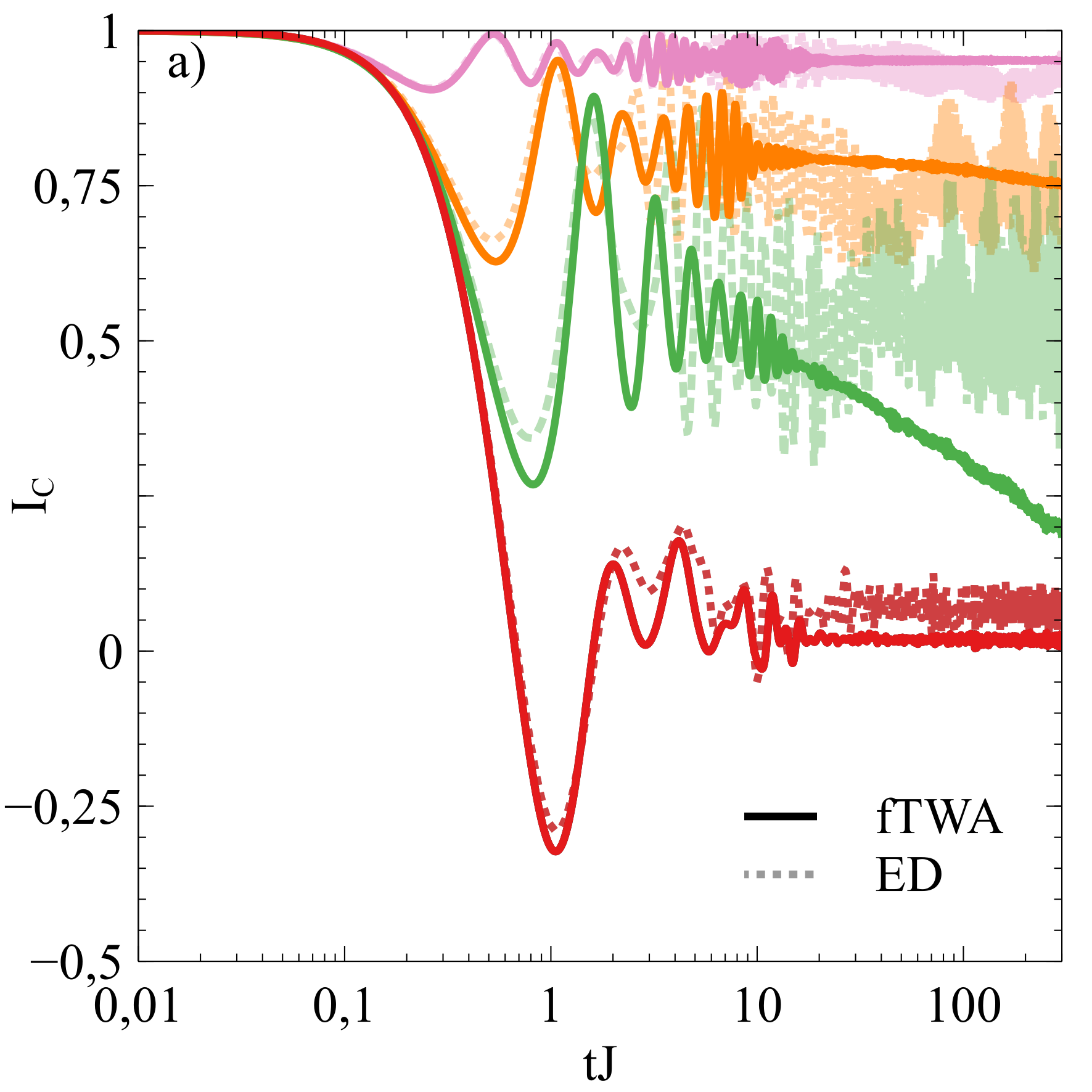
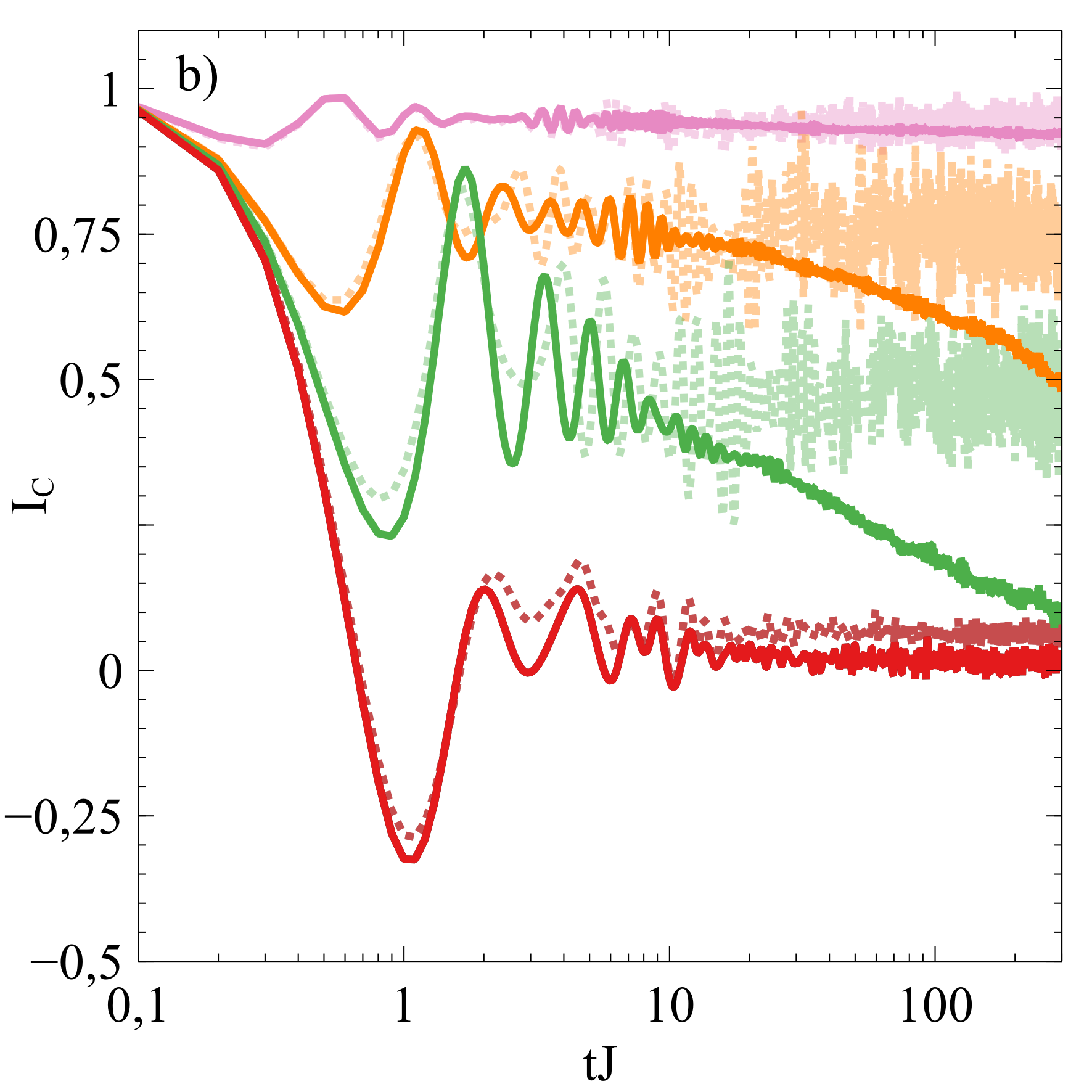
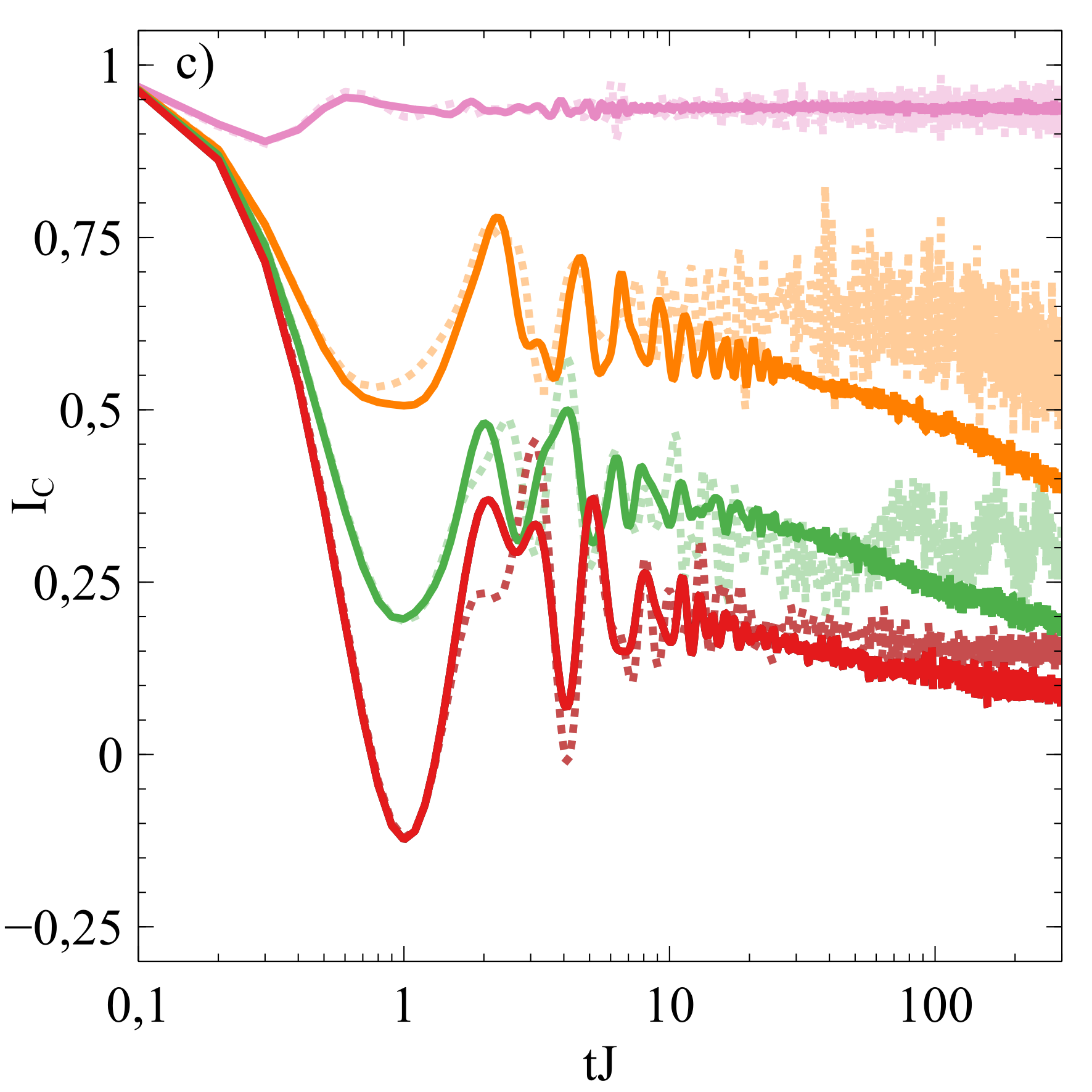
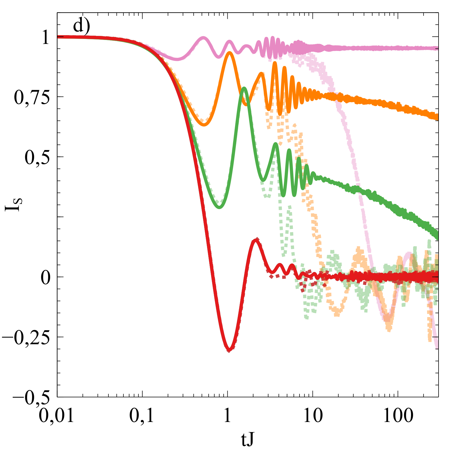
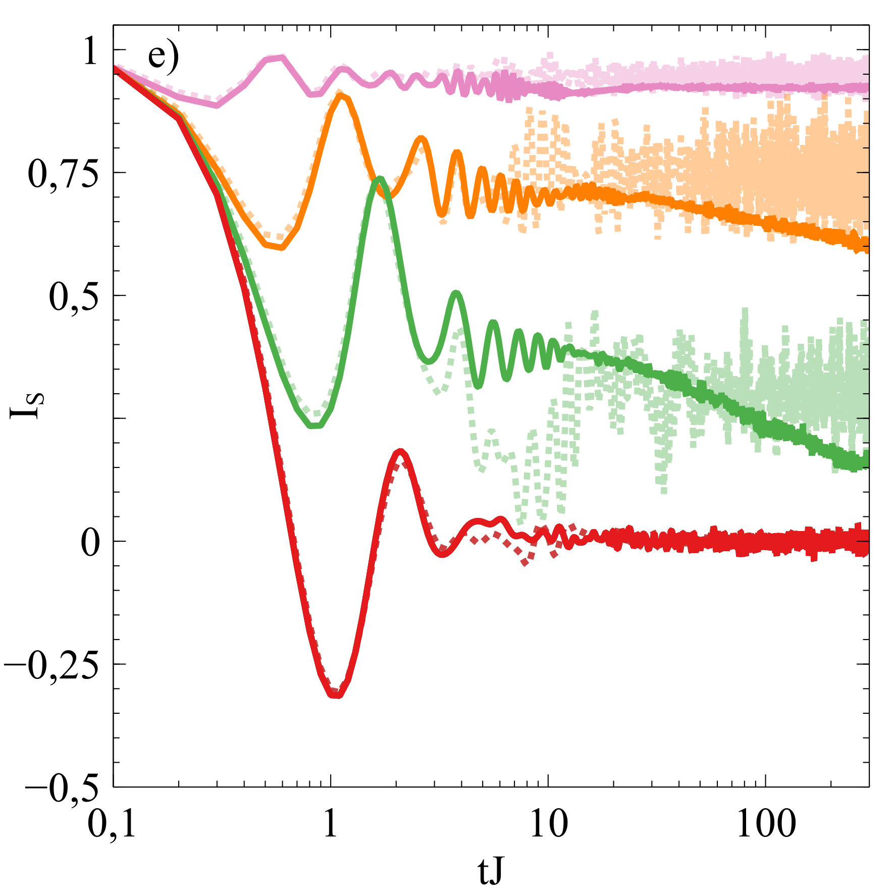
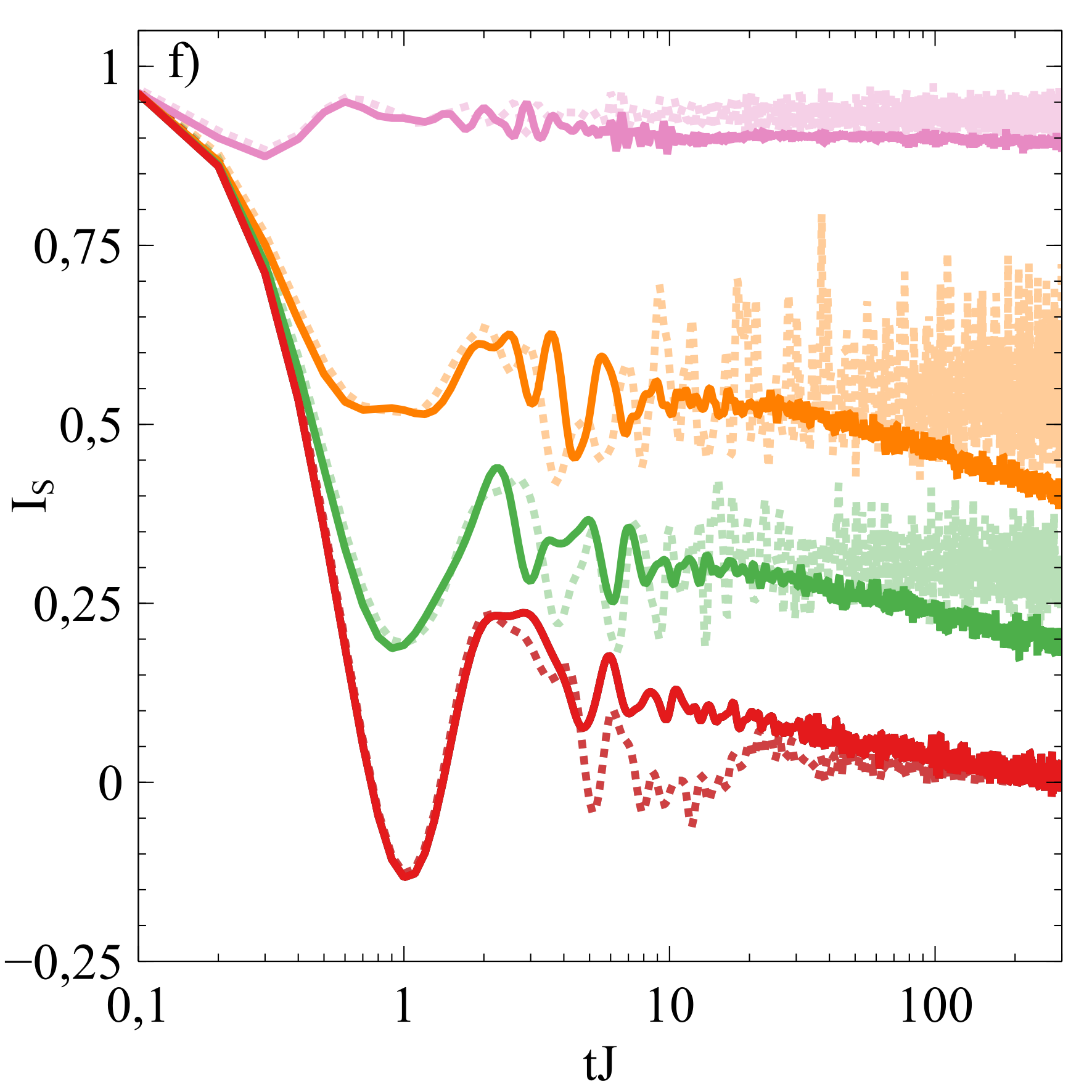
Figure 1: Time dependences of imbalance functions for charges (Fig. a-c) and spins (Fig. d-f). In each plot different strengths of the linear potential $\Delta_{1}/J$ are taken, i.e. $\Delta_{1}/J=1,\,4,\,6,\,12$ from the bottom to top. The dashed lines indicate the fTWA, while solid lines correspond to the ED results. The first column (a and d) corresponds to $A=1$, $\Delta_{2}=0$, the second column (b and e) to $A=0.9$, $\Delta_{2}=0$, and the third column (c and f) to $A=0.9$, $\Delta_{2}/J=0.5$. Simulations are performed for the one-dimensional system with 8 sites and with the CDW (a-c) or SDW (d-f) initial conditions. The other parameters are $U/J=1$, $j_{0}=4$, the number of trajectories used in fTWA is 1000 or higher. Preliminary results of (a) were obtained in (Kaczmarek, 2022).

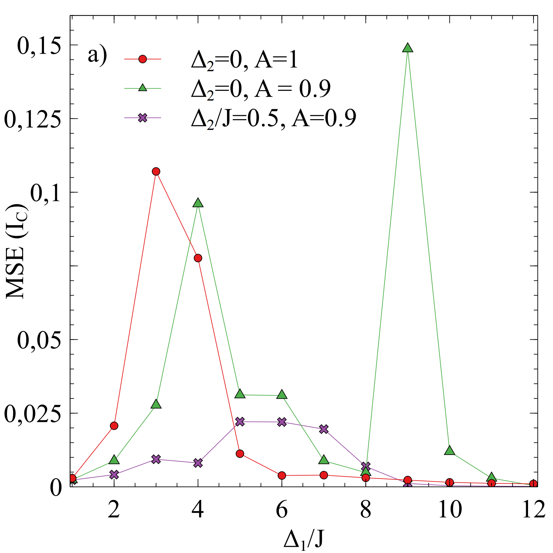
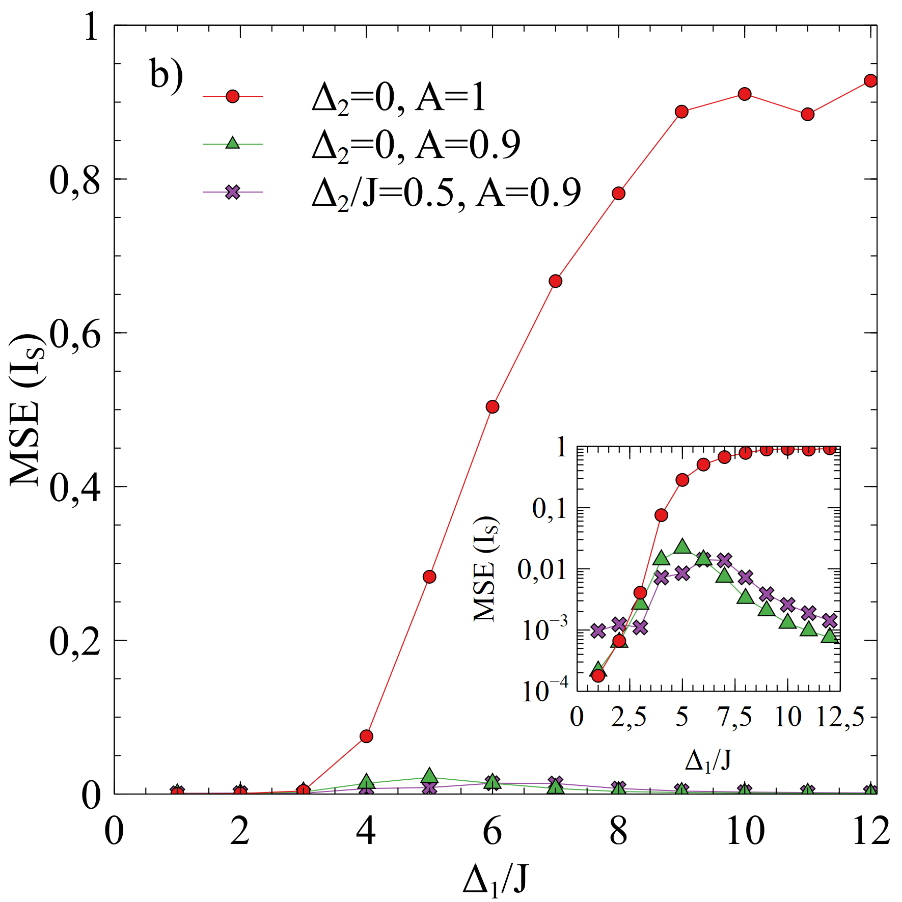
Figure 2: Dependence of the mean square error MSE($I_{C/S}$) on the linear potential strength $\Delta_{1}/J$ (for MSE($I_{C/S}$) definition, see Eq. (9)). MSE($I_{C}$) and MSE($I_{S}$) are calculated for charge (a) and spin (b) imbalance, respectively. Different parameter ranges are considered, circles correspond to $A=1$, $\Delta_{2}/J=0$, triangles to $A=0.9$, $\Delta_{2}/J=0$ and crosses to $A=0.9$, $\Delta_{2}/J=0.5$. In the inset of (b) we plotted the same data as in (b) but with an additional logarithmic scale in the vertical axis. The other parameters are the same as in Fig. 1.

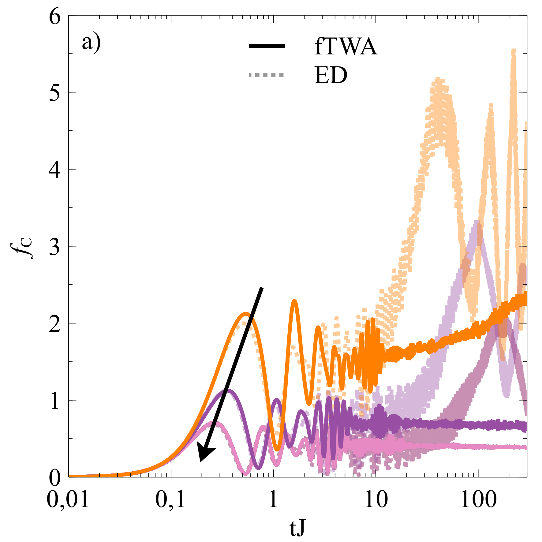
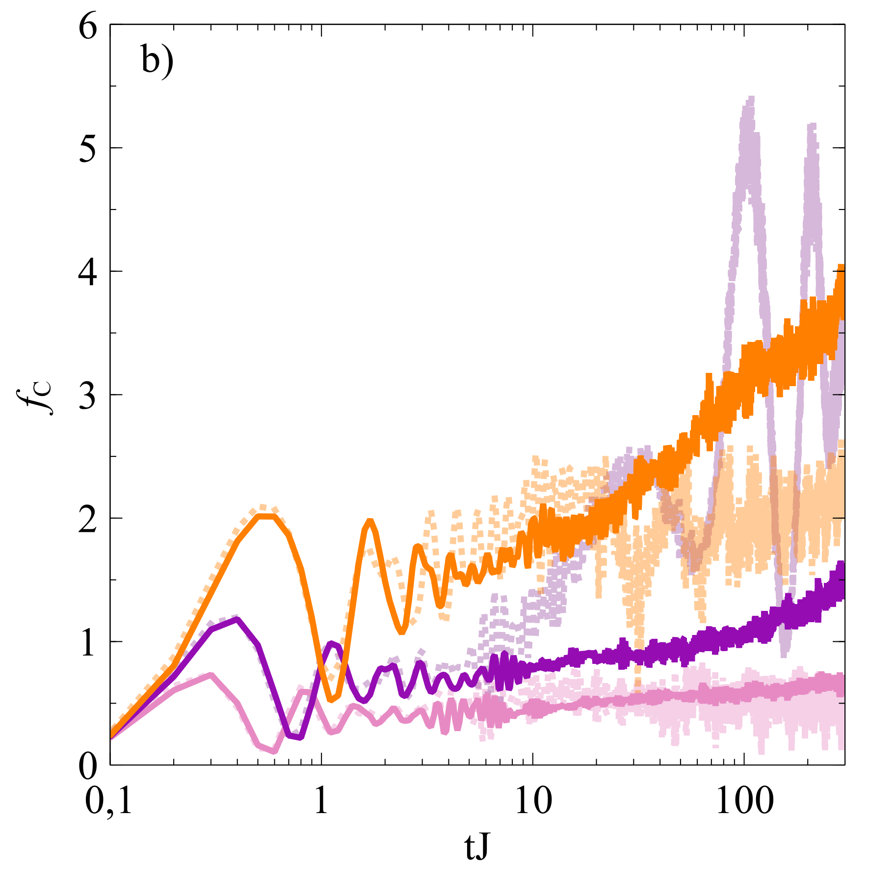
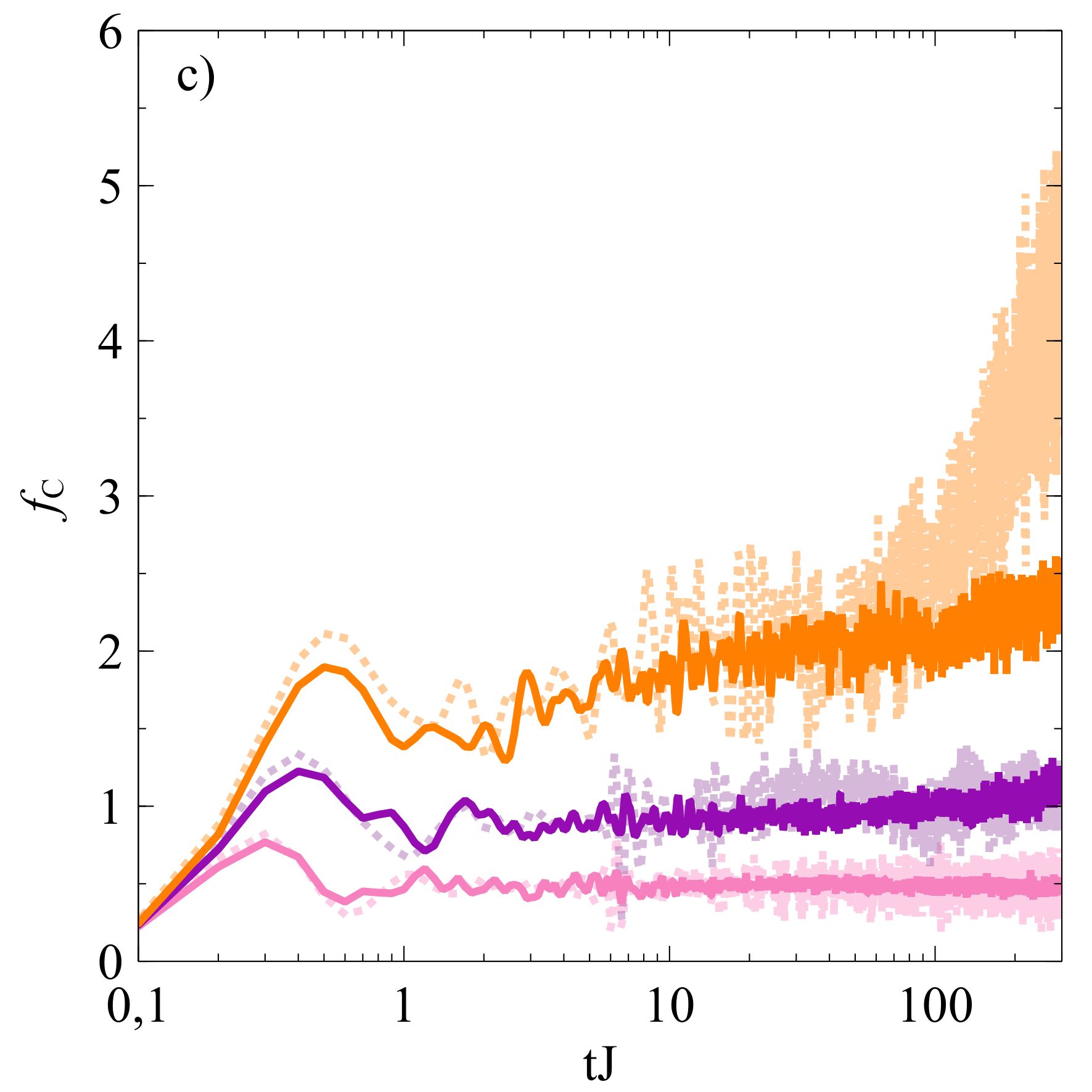
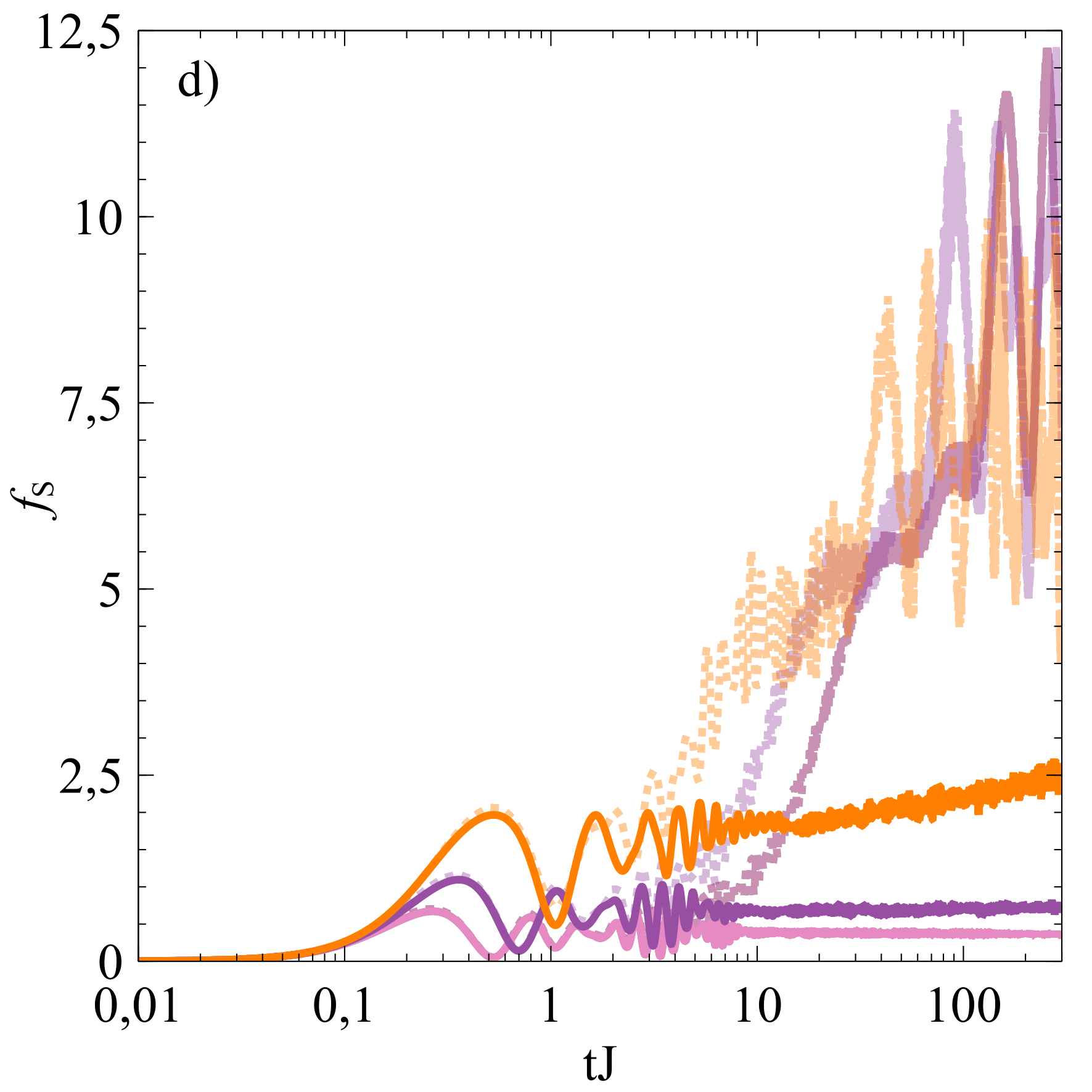
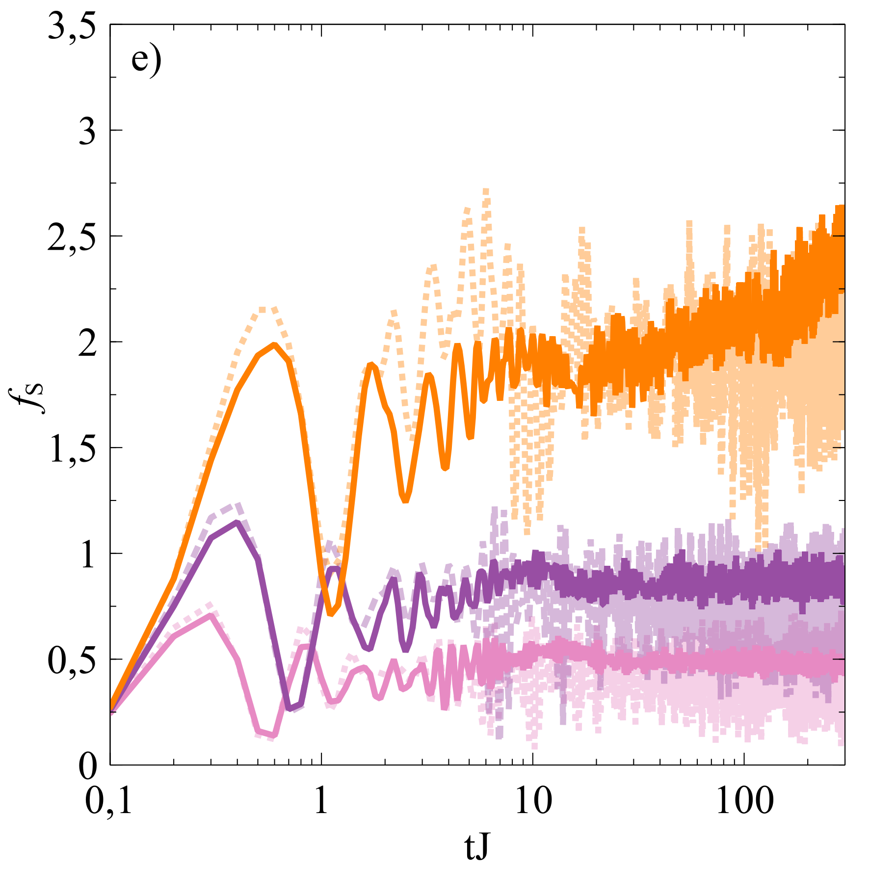
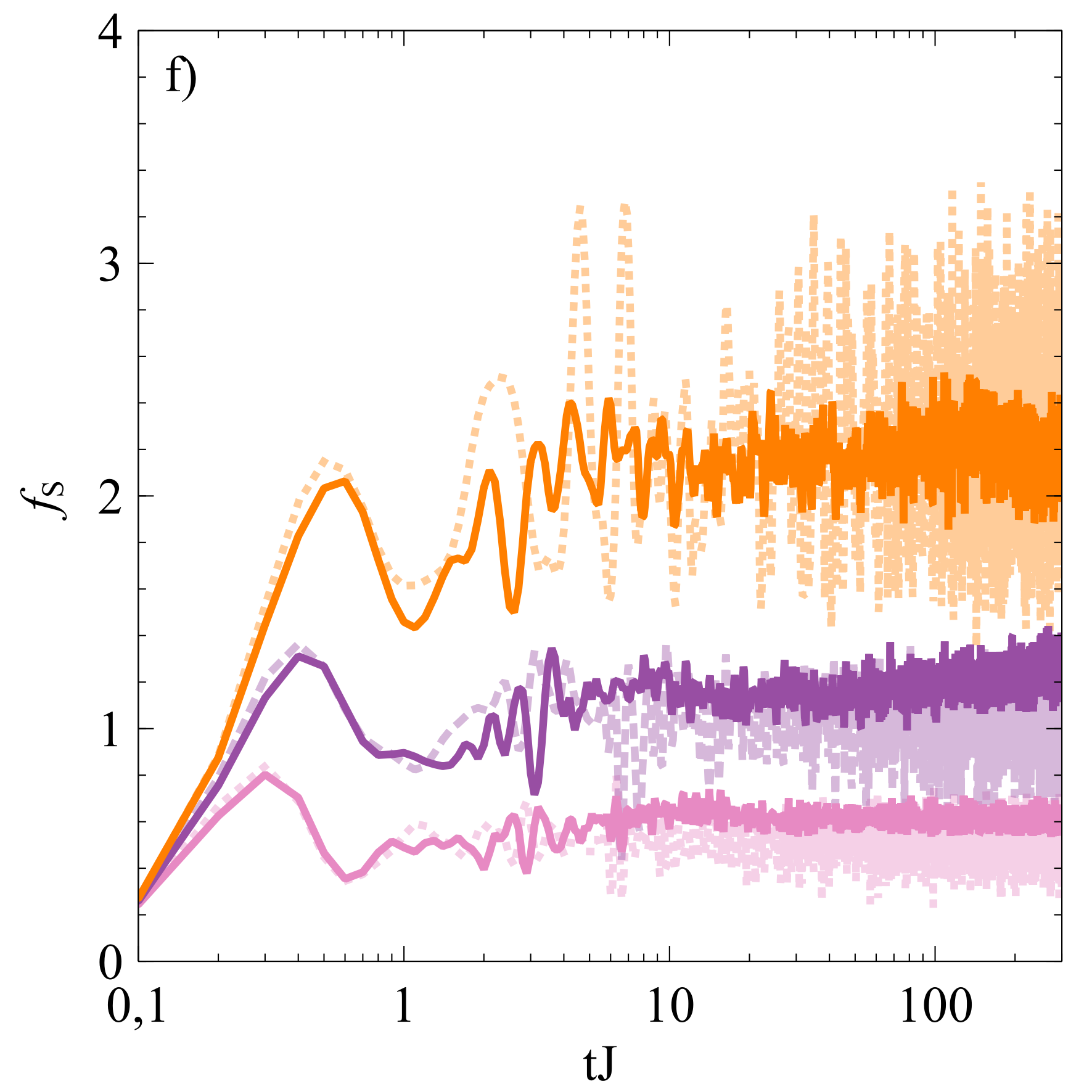
Figure 3: Time dependence of QFI for charges (Fig. a-c) and spins (Fig. d-f). In each plot different strengths of the linear potential $\Delta_{1}/J$ are taken, i.e. $\Delta_{1}/J=6,\,9,\,12$ from the top to bottom (direction of increasing values of $\Delta_{1}/J$ is marked by the arrow in Fig. a). The other parameters are the same as in Fig. 1.

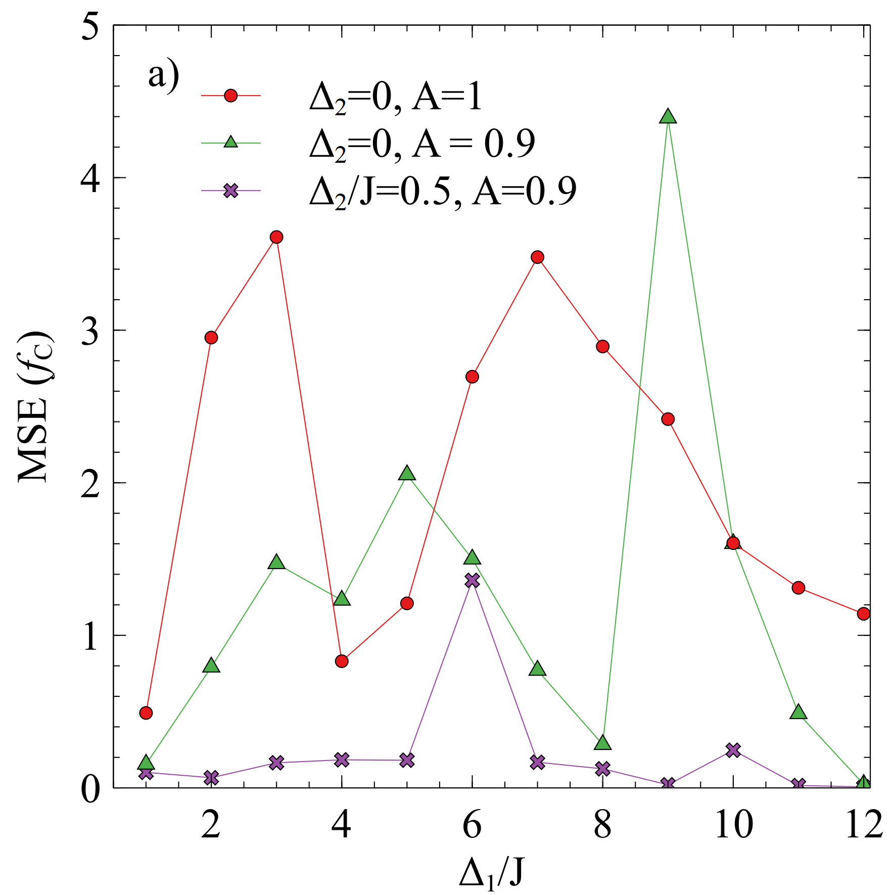
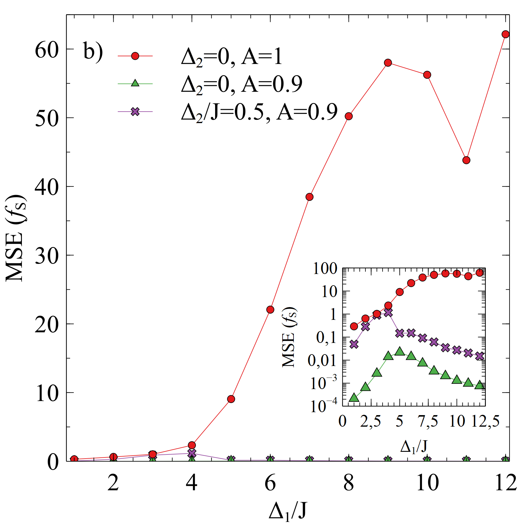
Figure 4: Dependence of the MSE($f_{C/S}$) on the linear potential strength $\Delta_{1}$. MSE($f_{C}$) and MSE($f_{S}$) are calculated for charge (a) and spin (b) QFI, respectively. Different parameter ranges are considered, circles correspond to $A=1$, $\Delta_{2}/J=0$, triangles to $A=0.9$, $\Delta_{2}/J=0$ and crosses to $A=0.9$, $\Delta_{2}/J=0.5$. In the inset of (b) we plotted the same data as in (b) but with an additional logarithmic scale in the vertical axis. The other parameters are the same as in Fig. 1.

To benchmark the fTWA method, we compare the results of semiclassical simulations with those of ED in a finite one-dimensional system at half-filling (8 lattice sites are investigated). The role of harmonic potential and spin dependence of the linear field is stressed by using the imbalance functions and QFI. We chose these quantities because they are accessible experimentally in trapped atoms and ions experiments and are useful in a discussion of ergodicity breaking in different systems (Schreiber et al., 2015; y. Choi et al., 2016; Bordia et al., 2016, 2017; Lüschen et al., 2017; Smith et al., 2016, 2019).

The imbalance function measures the distribution of charges (densities) and spin degrees of freedom at a given time. Assuming that the system starts from a charge density wave (CDW) where the even sites are doubly occupied and the odd ones are empty, the imbalance $I_{C}$ is defined as

$$I_{C}=\frac{1}{N}\left(\left\langle\hat{C}_{e}\right\rangle-\left\langle\hat{C}_{o}\right\rangle\right),$$ (5)

with

$$\hat{C}_{e/o}=\sum_{i\in\text{even/odd sites}}\hat{c}_{i},$$ (6)

where $\hat{c}_{i}=\hat{n}_{i\uparrow}+\hat{n}_{i\downarrow}$ is the local charge density, $N$ is the number of fermions, $\hat{C}_{e}$ and $\hat{C}_{o}$ are the operators of the total charge on even and odd sites, respectively.

Correspondingly, for the spin degrees of freedom, the imbalance function $I_{S}$ can be defined in the following way

$$I_{S}=\frac{1}{N}\left(\left\langle\hat{S}_{e}\right\rangle-\left\langle\hat{S}_{o}\right\rangle\right),$$ (7)

with

$$\hat{S}_{e/o}=\sum_{i\in\text{even/odd sites}}\hat{s}_{i},$$ (8)

where $\hat{s}_{i}=\hat{n}_{i\uparrow}-\hat{n}_{i\downarrow}$ is the local spin magnetization, $\hat{S}_{e}$ and $\hat{S}_{o}$ are the operators of the total spin magnetizaton (z component) on even and odd sites, respectively. In order to study the dynamics of the spin degrees of freedom we chose the initial spin density wave (SDW), i.e. even (odd) sites containing fermions with spins up (down).

Moreover, to efficiently discuss a quantitative difference between fTWA and ED, the mean square error (MSE) is analyzed, given by the formula

$$\text{MSE}(I_{C/S})=\frac{1}{N_{\text{s}}+1}\sum_{j=0}^{N_{\text{s}}}\left(I_{C/S}^{\text{ED}}(j\Delta t)-I_{C/S}^{\text{fTWA}}(j\Delta t)\right)^{2},$$ (9)

where $\Delta t=0.01/J$ is the time step after which data are numerically collected, $N_{\text{s}}\Delta t=300/J$ is the total time of simulations, $C$ and $S$ indices correspond to the charge and spin channel, respectively. Correspondingly, $I_{C/S}^{\text{ED}}$ and $I_{C/S}^{\text{fTWA}}$ stand for the imbalances calculated by using the ED and fTWA methods.

In Fig. 1 we plot the time dependences of the imbalances $I_{C}$ and $I_{S}$ in the fTWA and ED simulations. We first focus on the role of spin dependence of the linear potential. It is easily seen that for a spin-independent potential, $A=1$ (see Fig. 1 a and d), delocalization of spin degrees of freedom takes place (Fig. 1 d). A similar behavior was previously observed in the context of the spin-independent disordered systems (Prelovšek et al., 2016; Kozarzewski et al., 2018; Zakrzewski and Delande, 2018; Protopopov and Abanin, 2019; Środa et al., 2019; Suthar et al., 2020). In our simulations, this happens at times of the order of $\mathcal{O}(\text{tJ})$ and makes the fTWA to completely fail to describe the many-body quantum dynamics in the intermediate and large linear potential strength limit (see also the growth of MSE($I_{S}$) function in Fig. 2 b). In Fig. 1 e, we show that introduction of a weak spin dependence of the linear potential, i.e. $A=0.9$, forbids spin delocalization within the analyzed times and recovers the approximate predictability of fTWA.

Having established an efficient description of the spin channel, we focus on the role of harmonic potential in our semiclassical dynamics by setting $\Delta_{2}/J=0.5$ (see, Fig. 1 c and f). Then the situation is reversed to that of the spin channel. We observe enhancement of fTWA prediction in the charge channel which is explicitly seen in MSE($I_{C}$) for intermediate and large linear potential strength (see, Fig. 2 a).

In our studies we also look at the QFI which is a higher order correlation function in comparison to imbalance (QFI is proportional to the variance of $\hat{C}_{e}-\hat{C}_{o}$ or $\hat{S}_{e}-\hat{S}_{o}$). For pure initial states analyzed here, i.e. for CDW and SDW, the corresponding normalized QFI for charges $f_{C}$ and spins $f_{S}$ has the form (Braunstein and Caves, 1994; Hyllus et al., 2012; Tóth, 2012; Hauke et al., 2016)

$$f_{C}=\frac{4}{N}\left[\left\langle\left(\hat{C}_{e}-\hat{C}_{o}\right)^{2}\right\rangle-\left\langle\hat{C}_{e}-\hat{C}_{o}\right\rangle^{2}\right],$$ (10)

$$f_{S}=\frac{4}{N}\left[\left\langle\left(\hat{S}_{e}-\hat{S}_{o}\right)^{2}\right\rangle-\left\langle\hat{S}_{e}-\hat{S}_{o}\right\rangle^{2}\right].$$ (11)

Similarly as in the imbalance case we focus on the three regimes: (i) with spin-independent tilt ($A=1$) and without a harmonic potential ($\Delta_{2}=0$), see Fig. 3 a and d, (ii) with spin-dependent tilt ($A=0.9$) and without a harmonic potential ($\Delta_{2}=0$), see Fig. 3 b and e, (iii) with spin-dependent tilt ($A=0.9$) and with a harmonic potential ($\Delta_{2}=0.5$), see Fig. 3 c and f. The predictability of fTWA for QFI in (i) case is even worse than for the imbalance function. The abrupt increase in QFI at later times is not properly described in terms of semiclassical description. However introduction of the spin-dependent tilt and a harmonic potential substantially improves the fTWA method. This conclusion is better illustrated in Fig. 4 where MSE($f_{C/S}$) is plotted (definition of MSE($f_{C/S}$) corresponds to that given in Eq. (9) for imbalance). We observe that $f_{C}$ is mostly improved for the case $A=0.9$ and $\Delta_{2}=0.5$, while for $f_{S}$ the highest enhancement of the fTWA method is observed in the case of the spin-dependent linear potential. The latter behavior is consistent with that of the imbalance function for a spin channel (cf Fig. 1 d, f).

Interestingly, in the systems with a spin-dependent linear field and with an additional harmonic potential (($iii$) regime), the MSE of imbalance functions and QFI show a peak at the intermediate value of the linear potential strength. It means that fTWA gives the best prediction of quantum dynamics for weak and strong tilts. Such a feature was previously also observed for disordered systems when the disorder strength was varied (Acevedo et al., 2017; Sajna and Polkovnikov, 2020). Moreover, we also noticed that in the ($iii$) regime and charge channel, fTWA imbalances decay faster than the corresponding ones in ED, which suggests that fTWA dynamics can be regarded as an upper bound for relaxation rates. This situation is similar to that of disordered systems studied recently for spinless interacting fermions Iwanek et al. (2022).

IV Semiclassical dynamics of a two-dimensional system

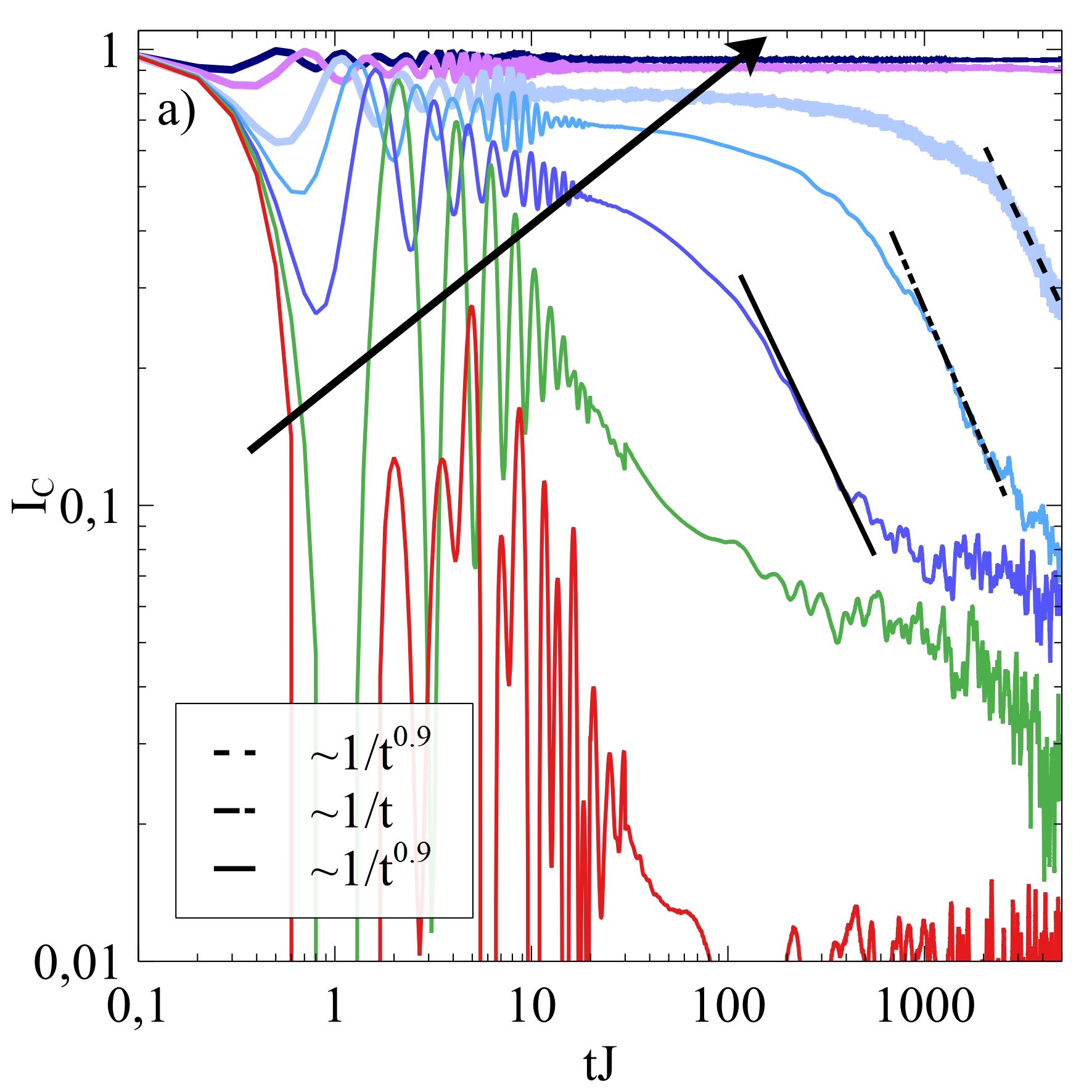
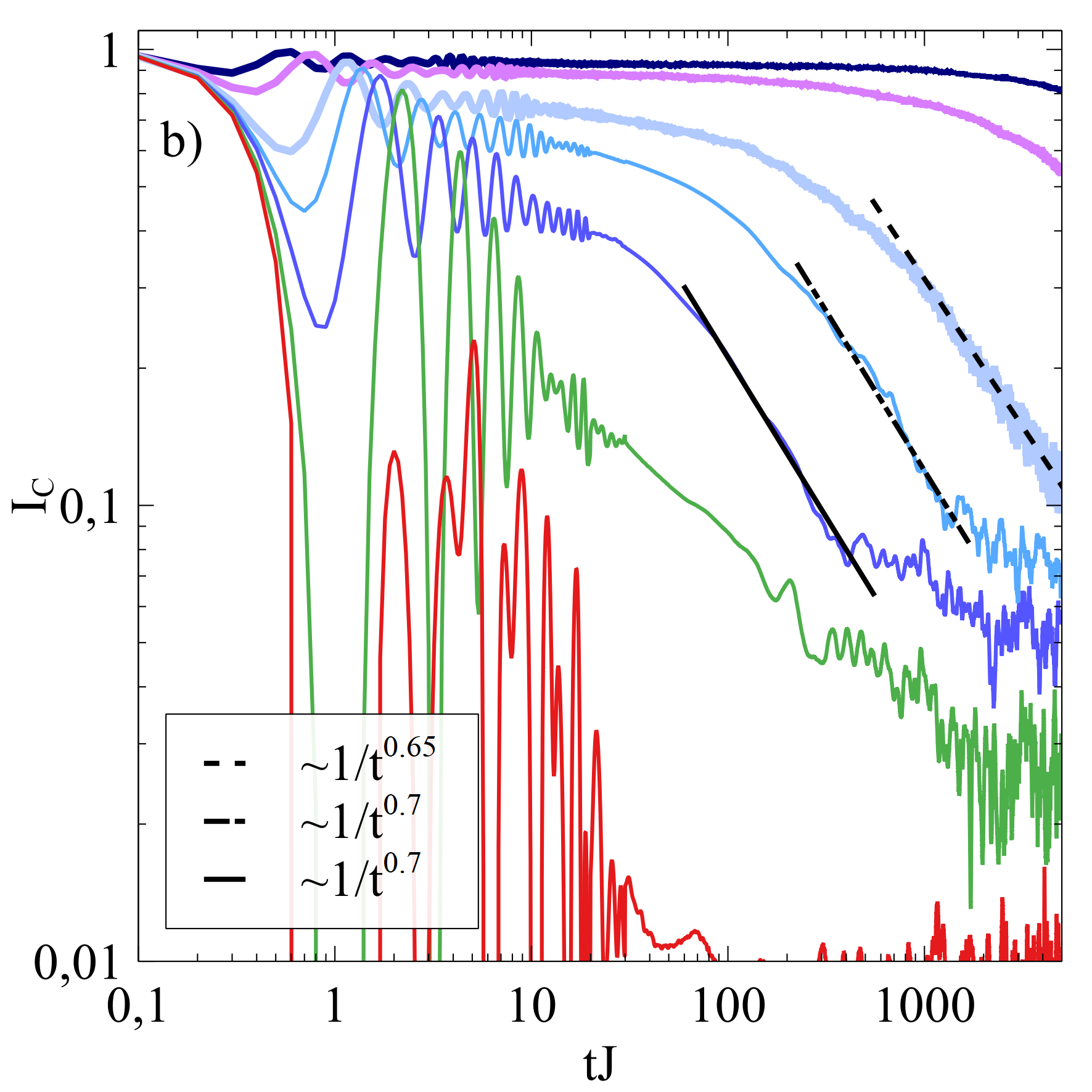
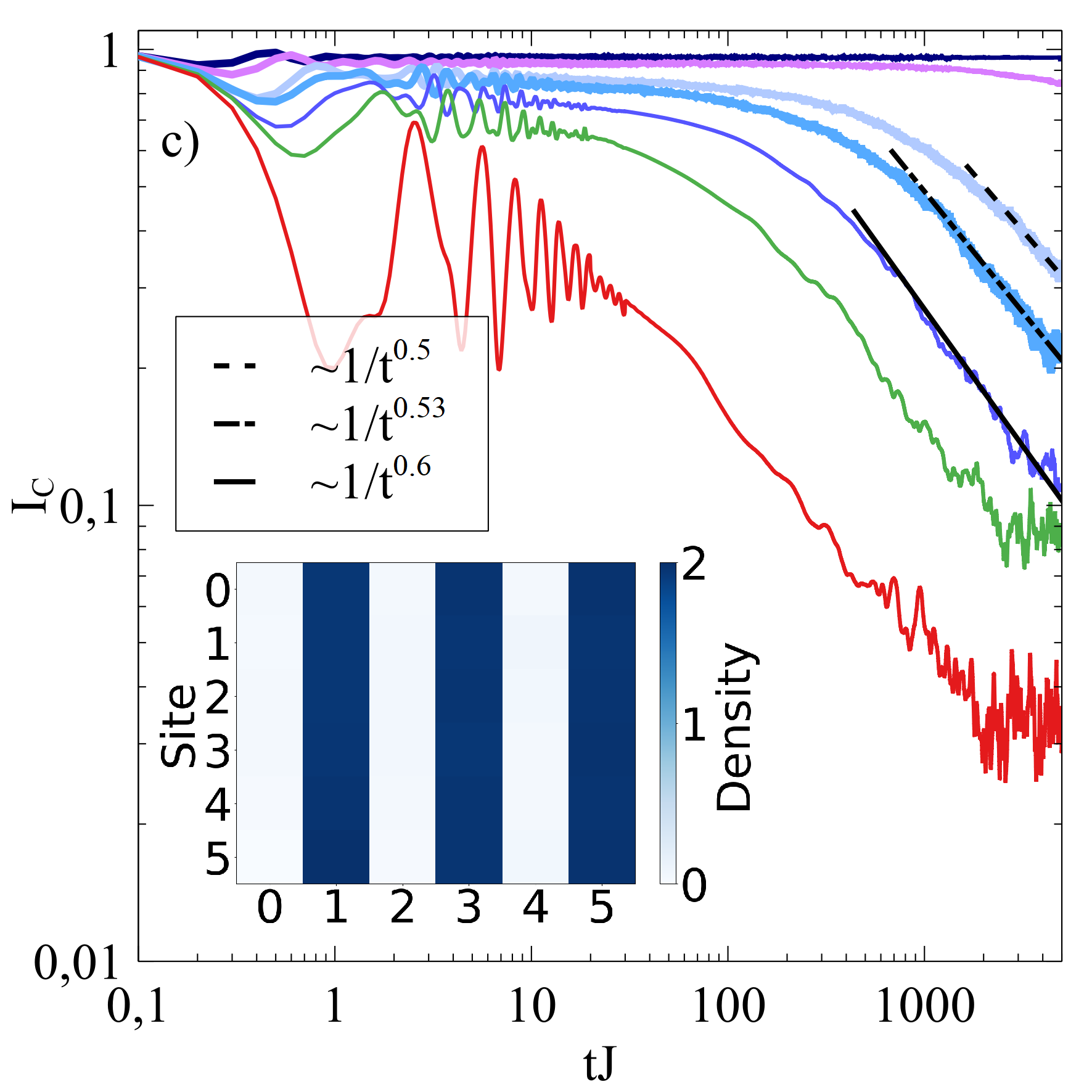
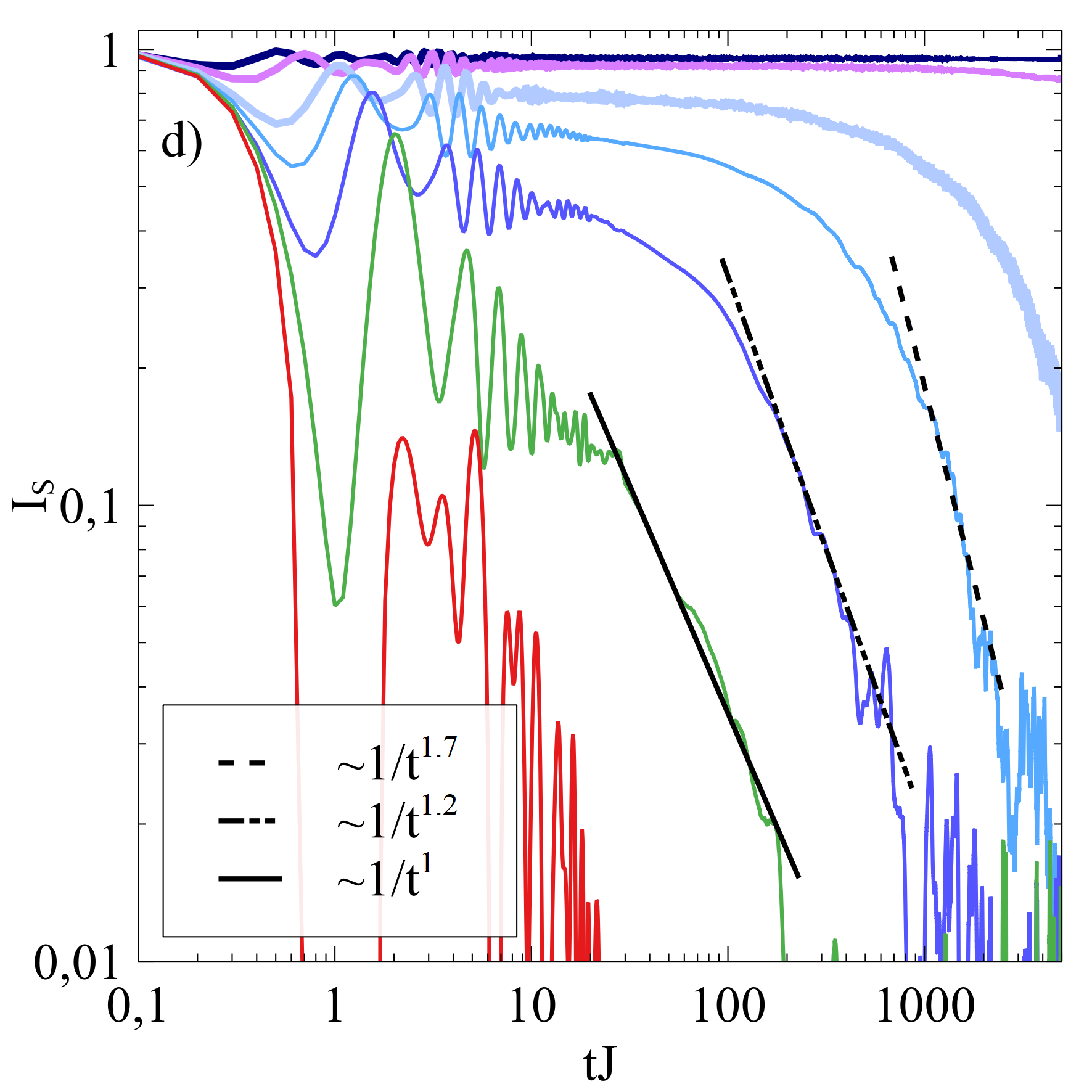
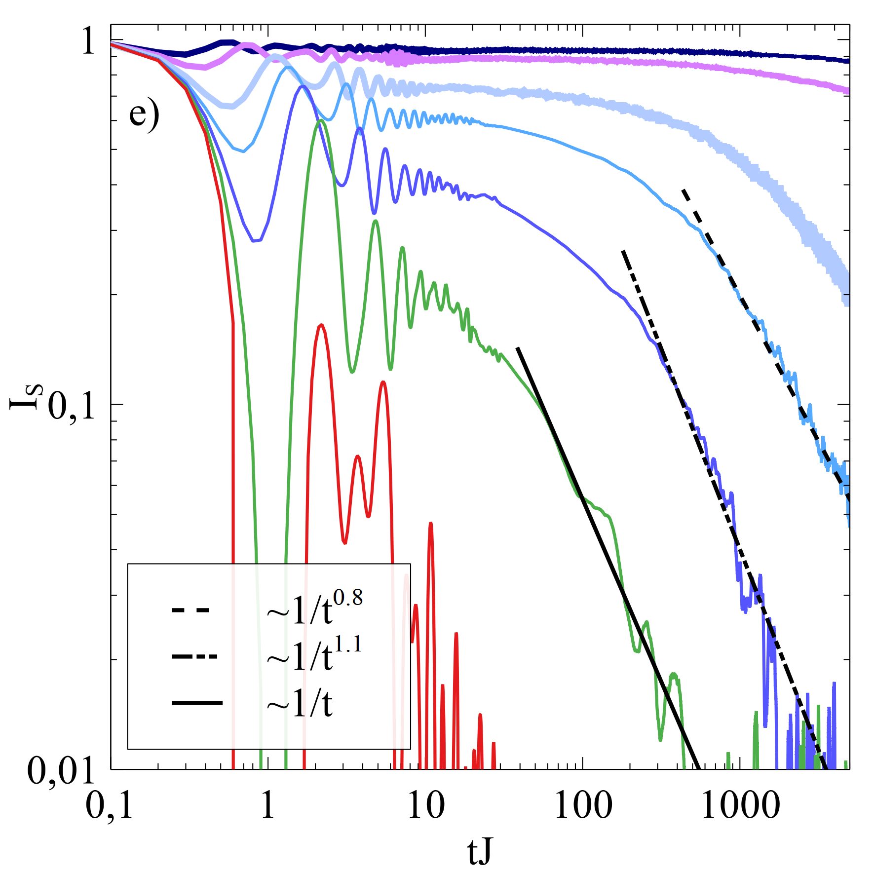
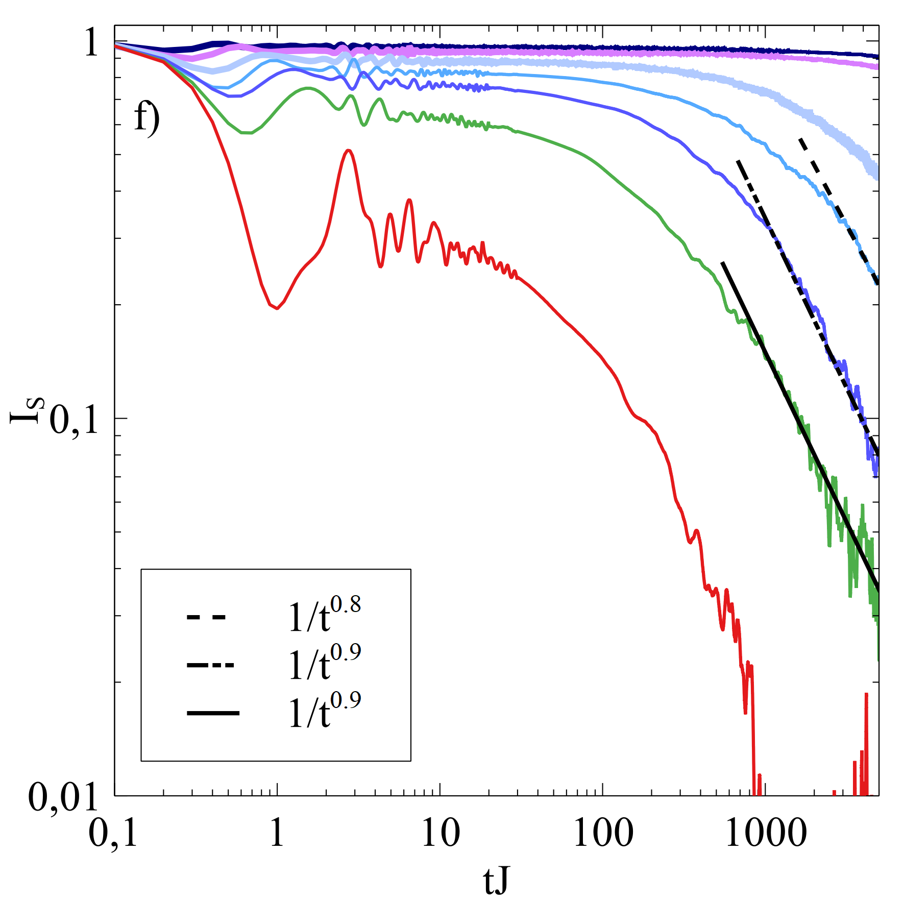
Figure 5: Time dependences of charge (Fig. a-c) and spin (Fig. d-f) imbalance functions. In each plot, different strengths of the linear potential $\Delta_{1}/J$ are taken, i.e. $\Delta_{1}/J=1,\,3,\,4,\,5,\,6,\,9,\,12$ from the bottom to top (direction of increasing values of $\Delta_{1}/J$ is marked by the arrow in Fig. a). The first column (a and d) corresponds to $A=1$, $\Delta_{2}=0$, the second column (b and e) to $A=0.9$, $\Delta_{2}=0$, the third column (c and f) to $A=0.9$, $\Delta_{2}/J=0.5$. Simulations are performed for a finite two-dimensional system with $6\times 6$ sites and with the striped CDW (a-c) or SDW (d-f) initial conditions. The structure of stripe-like initial conditions is presented in the inset of Fig. (c). The other parameters are $U/J=1$, $j_{x,0}=$ $j_{y,0}=0$, the number of trajectories used in fTWA is around 100.

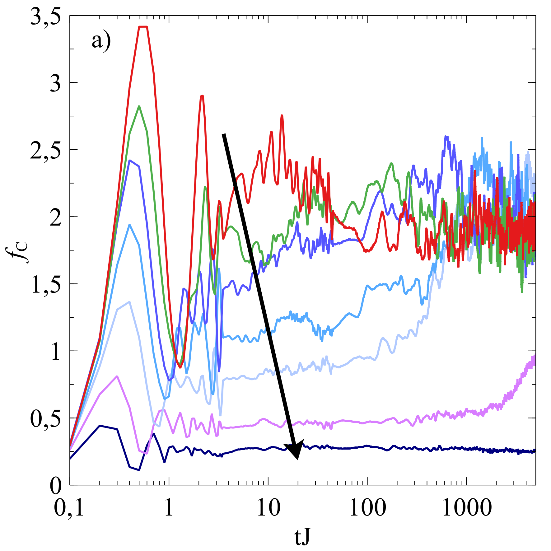
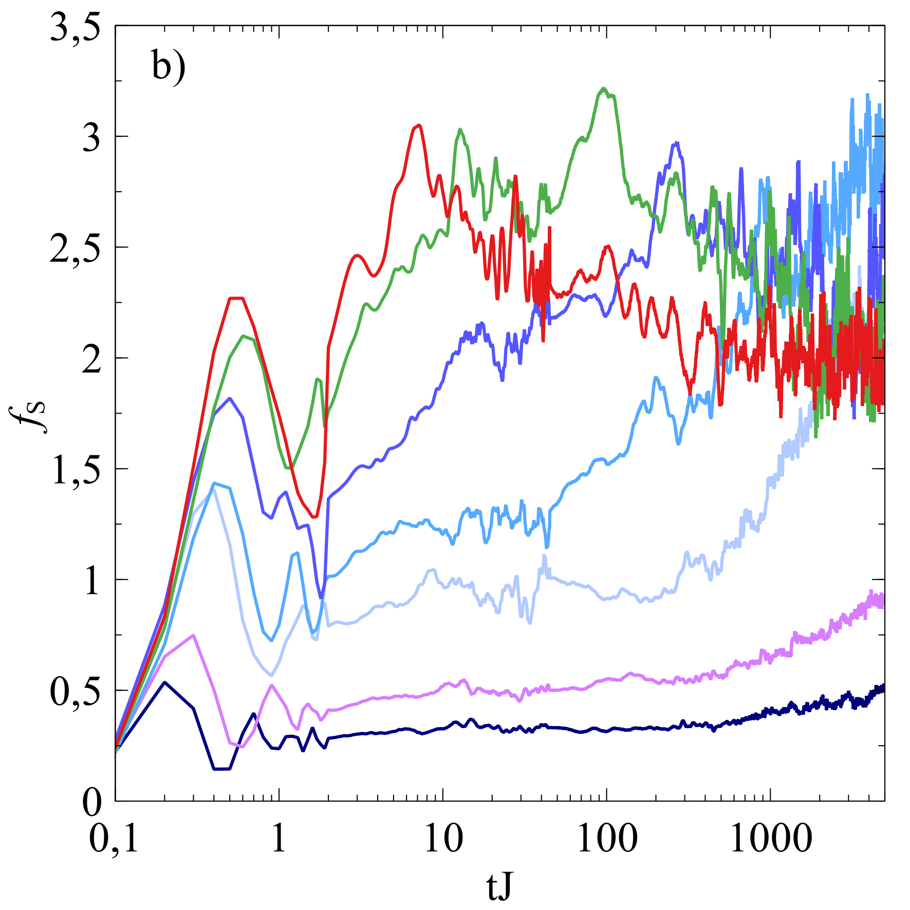
Figure 6: Time dependence of QFI for charges (a) and spins (b). The other parameters and denotation are the same as in Fig. 5, however here, increasing values of $\Delta_{1}/J$ correspond to the curves from the top to bottom (direction of increasing values of $\Delta_{1}/J$ is marked by the arrow in Fig. a).

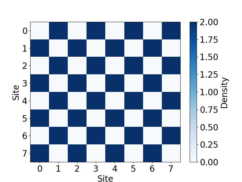
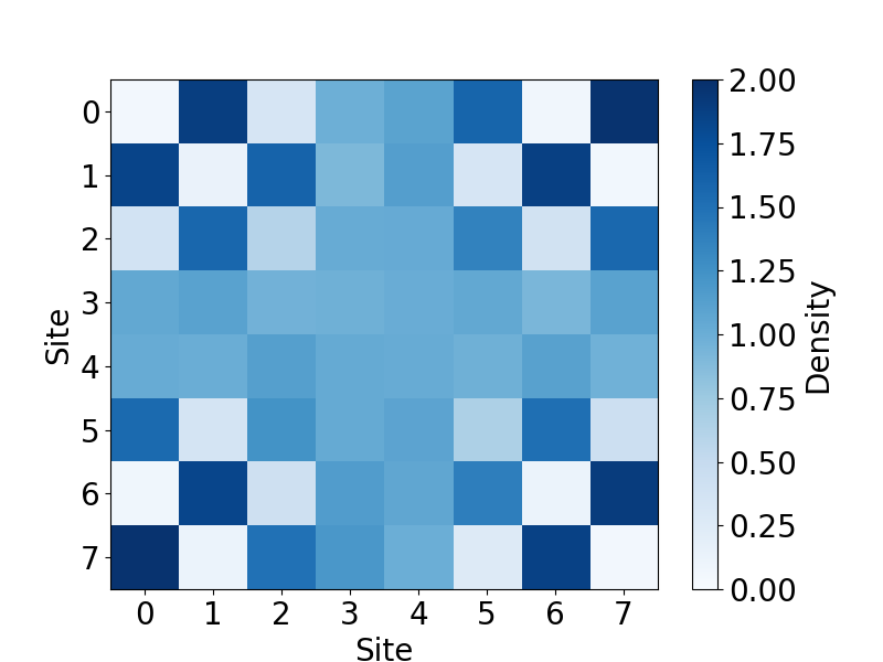
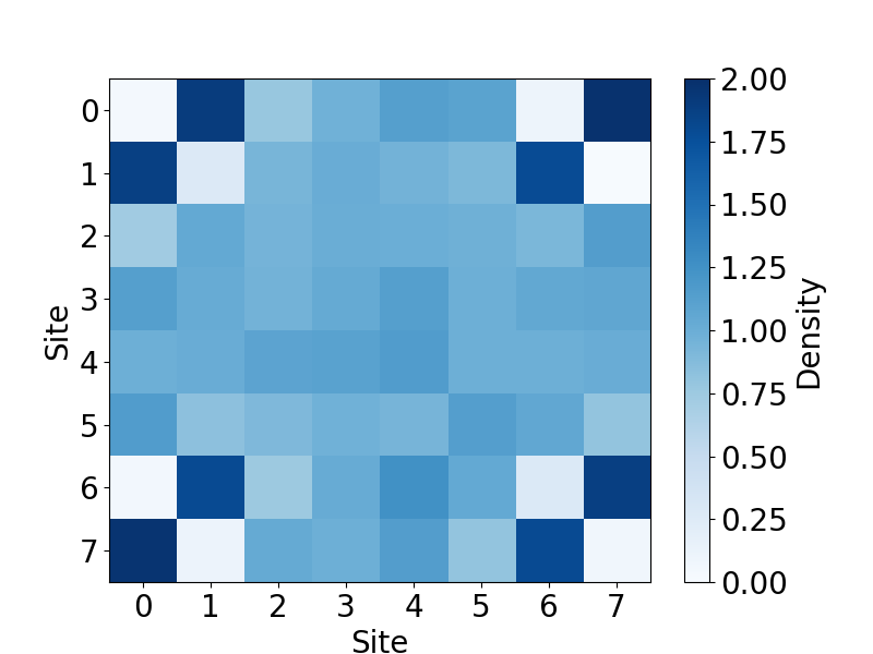
Figure 7: Density plots of charge distribution for $8\times 8$ square lattice at different times $tJ=0$ (left), $tJ=10$ (center), $tJ=300$ (right). In simulations $\Delta_{1x}=\Delta_{1y}=\Delta_{1}$ is chosen and around 100 fTWA trajectories are used in each plot. The other parameters are $U/J=1$, $A=0.9$, $\Delta_{1}/J=-6$, $\Delta_{2}/J=2$, $j_{0x}=j_{0y}=2$.

After benchmarking fTWA against the exact simulations, we focus our analysis on the system sizes that are beyond the reach of ED. Using the advantage offered by the fTWA method, that is the fact that it can be easily extended to higher dimensional systems, we focus on the system with a square lattice. It is worth mentioning that higher dimensional lattices have a higher coordination number and we expected that performance of fTWA, as a semiclassical method, would be improved.

In Sec. III it was shown that the predictability of fTWA for the case with spin-independent linear potential can be questioned for longer times (especially as far as the spin degrees of freedom are concerned). However, we decided to include this case in our two-dimensional simulations in order to show that the slowing down of dynamical behavior through the spin dependence of the linear potential is also clearly observed in the semiclassical picture in two dimensions (similarly like in the ED case analyzed for Hubbard chain in the previous section).

For a two-dimensional lattice system, the on-site potential $\Delta(j,\sigma)$ which was introduced in Sec. II, has to be generalized to the two spatial directions, i.e.

$$\Delta(j,\sigma) =\Delta_{1x}\left(\delta_{\sigma\downarrow}+A\delta_{\sigma\uparrow}\right)j_{x}+\Delta_{2x}(j_{x}-j_{x,0})^{2}$$

$$+\Delta_{1y}\left(\delta_{\sigma\downarrow}+A\delta_{\sigma\uparrow}\right)j_{y}+\Delta_{2y}(j_{y}-j_{y,0})^{2}$$ (12)

where $j=(j_{x},j_{y})$ is now a vector indicating the location of a given lattice site (the $j_{x}$ and $j_{y}$ are the Cartesian coordinates in the $x$ and $y$ directions, respectively). The coordinates $j_{x,0}$ and $j_{y,0}$ denote the center of the harmonic potential. In order to avoid lattice directions for which there is no potential change, throughout most of the work, we assume that the strengths of linear potentials in the $x$ and $y$ directions are $\Delta_{1x}=\Delta_{1}$ and $\Delta_{1y}=\sqrt{2}\Delta_{1}$, respectively (van Nieuwenburg et al., 2019). However, for simplicity, the harmonic potential strength satisfies the condition $\Delta_{2x}=\Delta_{2y}=\Delta_{2}$. In Eq. (12) we also assumed that the spin dependence of the linear potential given by the parameter $A$ is the same for $x$ and $y$ lattice dimensions.

Firstly we analyze the behavior of imbalances $I_{C}$ and $I_{S}$ at long times for $6\times 6$ lattice. We set the initial conditions in the form of stripes (see inset in Fig. 5 c) which are directly accessible in ultracold atom experiments (Bordia et al., 2016, 2017). In the striped CDW initial state every second stripe is doubly occupied and the others are empty (in striped SDW every second stripe contains fermions with spin up and the other sites are filled with fermions with spin down). The choice of such initial conditions needs a comment because the definitions of $I_{C}$ and $I_{S}$ given in Sec. III have to be updated. Instead of Eq. (6) and (8), we introduce the following definitions of $\hat{C}$ and $\hat{S}$ operators

$$\hat{C}_{e/o}=\sum_{i\in\text{X}_{e/o}}\hat{c}_{i},\ \hat{S}_{e/o}=\sum_{i\in\text{Y}_{e/o}}\hat{s}_{i},$$ (13)

where $\text{X}_{e}$ ($\text{Y}_{e}$) and $\text{X}_{o}$ ($\text{Y}_{o}$) denote the sets of sites that are initially doubly occupied (fermions with spin up) and empty (fermions with spin down), respectively.

The outcome of the numerical simulations of $I_{C}$ and $I_{S}$ are presented in Fig. 5 in which the results of three physical situations corresponding to those in Fig. 1 are plotted. In the simulations parameters are chosen in such a way that the imbalance function without a tilt potential decays near zero suggesting ergodic behavior within the analyzed time scales. In each of the three cases (i-iii, see Sec. III), as expected, imbalance dynamics for $I_{C}$ and $I_{S}$ are slowing down when the strength of tilt is increased. We also observe that the relaxation of imbalances, after introducing a harmonic and spin-dependent linear potential, becomes slower for weak and intermediate tilts. To be more specific, in the charge channel and with the spin-independent linear potential ($A=1$), nearly diffusive dynamics of densities is observed at longer times, i.e. $I_{C}\sim t^{-\gamma}$ where $\gamma=1$ (Fig. 5 a). After introducing the spin dependence of the linear field ($A=0.9$), the subdiffusive behavior appears ($\gamma<1$) which is further strengthened by a harmonic potential (Fig. 5 b and c). It is worth noting that the subdiffusive behavior was also observed for two-dimensional interacting systems with a sufficiently strong disorder (Sajna and Polkovnikov, 2020; Lev and Reichman, 2016). For the spin degrees of freedom, the situation is more complex due to spin dependence of the linear potential. For the spin-independent tilt, spin transport is superdiffusive and approach diffusive when the spin dependence is imposed (5 d and e). Introduction of a harmonic potential makes the spin dynamics become subdiffusive, similarly like in the charge case. This is especially visible for higher values of the linear potential strength, see Fig. 5 c and f. Interestingly, the subdiffusive behavior of spin degrees of freedom was also observed in the disordered two-dimensional Hubbard model (Sajna and Polkovnikov, 2020). It is also worth mentioning, that some delocalization features of the initial striped CDW state with short-wavelength have been also recently reported in Ref. (Doggen et al., 2022). This is consistent with our studies, however, in Ref. (Doggen et al., 2022), different tilt direction and shorter time scales have been analyzed, therefore, direct comparison needs further investigation which we left for future studies.

It is important to mention that the fitting curves $t^{-\gamma}$ in Fig, 5 were obtained for the long-time limit and for three fixed values of $\Delta_{1}/J$. It is straightforward to notice that in Fig. 5 a and b there are significant deviations from these fitting curves at later times. It can be accounted for by significant finite-size effects in the dynamics, which is faster in the system without a harmonic potential, see Appendix VII. In Appendix VII we also explain that the finite size effects can be neglected in the cases when fTWA gives the lowest errors and when it mimics the behavior of disordered systems.

We also investigate $f_{C}$ and $f_{S}$ focusing on the limit in which fTWA satisfactorily describes the long-time dynamics, i.e. when the spin dependence ($A=0.9)$ and the harmonic potential ($\Delta_{2}=0.5$) are introduced. The results are presented in Fig. 6 for charge and a spin channels. Interestingly, in both situations we observe a logarithmic-like growth of QFI, which is slower for higher values of the linear potential. Here again as for imbalances, the dynamics of QFI is similar to that of strongly disordered systems in one and two dimensions (De Tomasi et al., 2019; Guo et al., 2020; Sajna and Polkovnikov, 2020) or that of tilted triangular ladders (Guo et al., 2021). In Appendix VII we also show that the finite-size effects do not play a significant role in the logarithmic growth and can be neglected.

In the end of this section we also look at the competition between the linear ($\Delta_{1}$) and harmonic ($\Delta_{2}$) potentials in the parameter range in which additional harmonicity of the lattice leads to the appearance of long-lived ergodic and non-ergodic regions. Fig. 7 presents the density plot of charge distribution on the lattice. At the expenses of shorter time analysis, we increase the size of the lattice to $8\times 8$ and set the lowest value of harmonic potential at the lattice center. To precisely catch the density decay on the individual sites we choose a checkerboard-like structure of the initial CDW-like state in which only charge channel is analyzed. In the presented simulations the linear potential is three times stronger than the harmonic and we simply choose $\Delta_{1x}=\Delta_{1y}=\Delta_{1}$. We observed that within the analyzed time scales, charges represented by doubly occupied sites, did not decay at the corners of the lattice. The corresponding phase separation has been also recently observed in the one-dimensional system in which the effective local field was used for explanation of such behavior (Yao et al., 2021a; Chanda et al., 2020; Yao and Zakrzewski, 2020; Morong et al., 2021).

V Summary and outlook

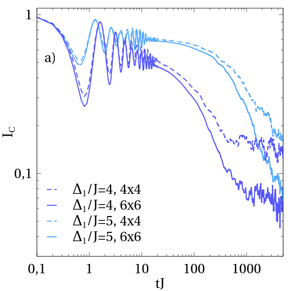
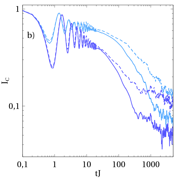
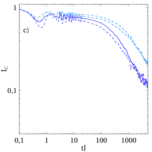
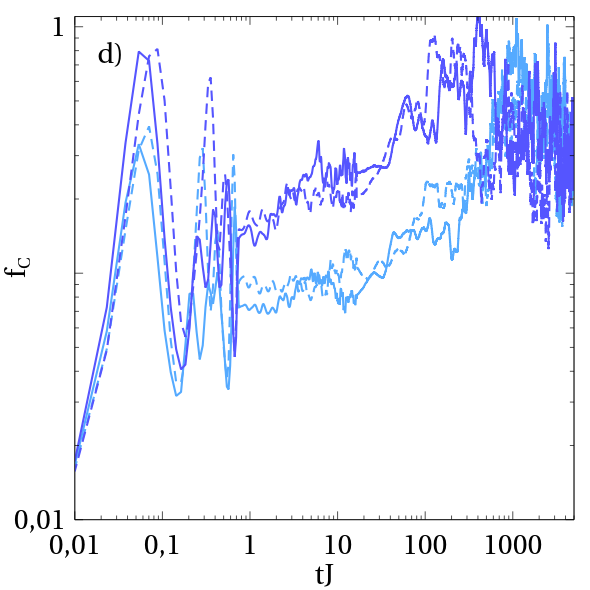
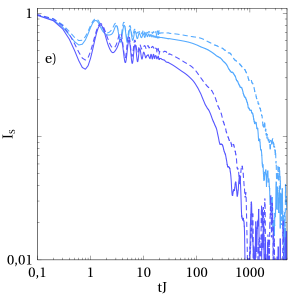
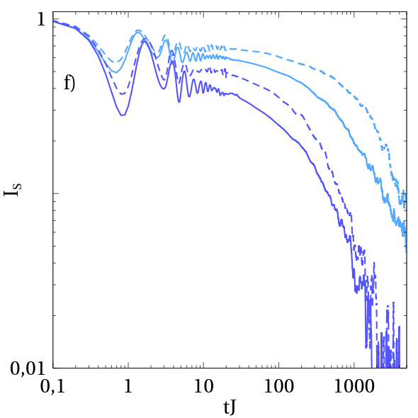
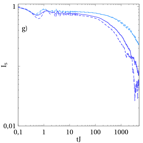
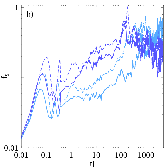
Figure 8: Imbalance $I_{C}$, $I_{S}$ and QFI $f_{C}$, $f_{S}$ functions for different lattice sizes: $4\times 4$ - dashed lines, $6\times 6$ - solid lines. In each figure the plots are made for the two values of tilt strength $\Delta_{1}/J=4$ (dark blue), $\Delta_{2}/J=5$ (light blue). The first row (Fig. a-d) represents the dynamics evaluated from the striped CDW initial condition, while the second row (Fig. e-f) represents the dynamics evaluated from the striped SDW initial condition. $U/J=1$ and about 100 fTWA trajectories where used for a simulation of each line.

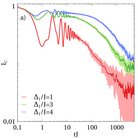
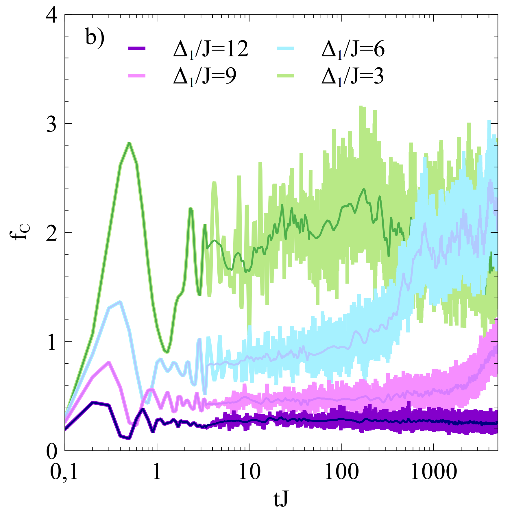
Figure 9: Charge imbalance $I_{C}$ (Fig. a) and QFI $f_{C}$ (Fig. b) for different values of the linear potential $\Delta_{1}/J$. Solid lines inside envelopes representing original data are obtained by filtering high frequency oscillation and fTWA noise. The data presented in (a) and (b) correspond to Fig. 5 c and Fig. 6 a for chosen values of $\Delta_{1}/J$.

In this work we show that for a certain range of parameters, the fTWA method can efficiently simulate quantum-many body dynamics for the tilted Hubbard model. This is the case when a harmonic and spin-dependent linear potentials are imposed. Interestingly we observe also that this improvement appears for higher-order correlation functions like QFI suggesting that this strictly non-meanfield result is very efficiently described by the quantum fluctuation included in fTWA.

These results enable us to discuss the many-body dynamics of the disorder-free two-dimensional square lattice. We show that quantum evolution of charge and spin degrees of freedom exhibits subdiffusive behavior which is similar to that of disorder systems (Lev and Reichman, 2016; Sajna and Polkovnikov, 2020) (however, in two-dimensional disordered systems a behavior somewhat faster than a power law one can be expected due to rare regions (Gopalakrishnan et al., 2016; Luitz and Lev, 2017; Doggen et al., 2020; Pöpperl et al., 2021)). Moreover, disorder-like dynamical behavior is also recovered for QFI which show a logarithmic-like growth (De Tomasi et al., 2019; Guo et al., 2020; Sajna and Polkovnikov, 2020). Next focusing our study on the on-site density dynamics, we show that the harmonic potential induces lattice locations at which the ergodic or non-ergodic type of behavior is observed. This result complements the recent studies in one dimension in which phase separation of ergodic and non-ergodic regions has been observed (Yao et al., 2021a; Chanda et al., 2020; Yao and Zakrzewski, 2020; Morong et al., 2021).

It is also worth pointing out that the spin dependence of the linear potential, controlled in our simulations by a parameter $A$, was similar to that of the recent experimental work in Ref. (Scherg et al., 2021). This suggests that the fTWA method can become an efficient tool for the theoretical prediction of real experimental data for larger system sizes.

In future studies it will be interesting to investigate other types of initial conditions like domain walls in two dimensions (Doggen et al., 2022) or other types of tilts that modify the lattice directions for which potential changes can be small (van Nieuwenburg et al., 2019). Moreover the harmonic potential strength analyzed in this work can induce anomalously slow dynamics in different parts of the lattice locations therefore it will be also interesting to look at the dynamics locally and test the local effective potential theory in the semiclassical picture (Yao et al., 2021b; Chanda et al., 2020; Yao and Zakrzewski, 2020; Yao et al., 2021a).

VI Acknowledgments

We would like to thank Marcin Mierzejewski for valuable discussions. A.S.S. acknowledges the funding from the Polish Ministry of Science and Higher Education through a ”Mobilność Plus” program nr 1651/MOB/V/2017/0. Numerical studies in this work have been carried out using resources provided by the Wroclaw Centre for Networking and Supercomputing , Grant No. 551, and in part also by PL-Grid Infrastructure.

VII Appendix: Finite-size effects

In Fig. 8 we present the finite-size effects for the imbalance function and QFI. Within the considered system sizes, we only see qualitative difference in these effects for the charge channel without an imposed harmonic potential (Fig. 8 a, b). Interestingly, in the limit of disorder-like behavior observed for the two-dimensional system, Fig. 8 c, d, g, h, the finite-size effects seem unimportant in the presented discussion.

VIII High frequency oscillations and noise

The dynamics presented in Figs. 9 was filtered from high frequency oscillations coming from inherit quantum dynamics on the tilted lattice and from spurious fTWA noise coming from sampling of the initial Wigner function. The spurious fTWA noise can be removed taking more fTWA trajectories, however, the application of filtering is less numerically costly than the simulation of more trajectories. We checked that addition of more fTWA trajectories does not change the filtered signal. To filter the obtained data a Kaiser window was used. An examplary original signal and its form after filtering are presented for $I_{C}$ and $f_{C}$ in Fig. 9.

References

- Abanin et al. (2019) D. A. Abanin, E. Altman, I. Bloch, and M. Serbyn, Rev. Mod. Phys. 91, 021001 (2019).
- Nandkishore and Huse (2015) R. Nandkishore and D. A. Huse, Annual Review of Condensed Matter Physics 6, 15 (2015).
- van Horssen et al. (2015) M. van Horssen, E. Levi, and J. P. Garrahan, Physical Review B 92, 100305(R) (2015).
- Gogolin and Eisert (2016) C. Gogolin and J. Eisert, Reports on Progress in Physics 79, 056001 (2016).
- Smith et al. (2017a) A. Smith, J. Knolle, D. L. Kovrizhin, and R. Moessner, Phys. Rev. Lett. 118, 266601 (2017a).
- Grover and Fisher (2014) T. Grover and M. P. A. Fisher, Journal of Statistical Mechanics: Theory and Experiment 2014, P10010 (2014).
- Smith et al. (2017b) A. Smith, J. Knolle, R. Moessner, and D. L. Kovrizhin, Phys. Rev. Lett. 119, 176601 (2017b).
- Khemani et al. (2020) V. Khemani, M. Hermele, and R. Nandkishore, Phys. Rev. B 101, 174204 (2020).
- Scherg et al. (2021) S. Scherg, T. Kohlert, P. Sala, F. Pollmann, B. H. Madhusudhana, I. Bloch, and M. Aidelsburger, Nature Communications 12 (2021), 10.1038/s41467-021-24726-0.
- Sala et al. (2020) P. Sala, T. Rakovszky, R. Verresen, M. Knap, and F. Pollmann, Phys. Rev. X 10, 011047 (2020).
- Gornyi et al. (2005) I. V. Gornyi, A. D. Mirlin, and D. G. Polyakov, Phys. Rev. Lett. 95, 206603 (2005).
- Basko et al. (2006) D. Basko, I. Aleiner, and B. Altshuler, Annals of Physics 321, 1126 (2006).
- Oganesyan and Huse (2007) V. Oganesyan and D. A. Huse, Phys. Rev. B 75, 155111 (2007).
- Luitz and Lev (2017) D. J. Luitz and Y. B. Lev, Annalen der Physik 529, 1600350 (2017).
- Serbyn et al. (2014) M. Serbyn, M. Knap, S. Gopalakrishnan, Z. Papić, N. Y. Yao, C. R. Laumann, D. A. Abanin, M. D. Lukin, and E. A. Demler, “Interferometric probes of many-body localization,” (2014).
- Laumann et al. (2015) C. Laumann, R. Moessner, A. Scardicchio, and S. Sondhi, The European Physical Journal Special Topics 224, 75 (2015).
- Smith et al. (2016) J. Smith, A. Lee, P. Richerme, B. Neyenhuis, P. W. Hess, P. Hauke, M. Heyl, D. A. Huse, and C. Monroe, Nature Physics 12, 907 (2016).
- Chiaro et al. (2022) B. Chiaro, C. Neill, A. Bohrdt, M. Filippone, F. Arute, K. Arya, R. Babbush, D. Bacon, J. Bardin, R. Barends, S. Boixo, D. Buell, B. Burkett, Y. Chen, Z. Chen, R. Collins, A. Dunsworth, E. Farhi, A. Fowler, B. Foxen, C. Gidney, M. Giustina, M. Harrigan, T. Huang, S. Isakov, E. Jeffrey, Z. Jiang, D. Kafri, K. Kechedzhi, J. Kelly, P. Klimov, A. Korotkov, F. Kostritsa, D. Landhuis, E. Lucero, J. McClean, X. Mi, A. Megrant, M. Mohseni, J. Mutus, M. McEwen, O. Naaman, M. Neeley, M. Niu, A. Petukhov, C. Quintana, N. Rubin, D. Sank, K. Satzinger, T. White, Z. Yao, P. Yeh, A. Zalcman, V. Smelyanskiy, H. Neven, S. Gopalakrishnan, D. Abanin, M. Knap, J. Martinis, and P. Roushan, Phys. Rev. Research 4, 013148 (2022).
- Schreiber et al. (2015) M. Schreiber, S. S. Hodgman, P. Bordia, H. P. Lüschen, M. H. Fischer, R. Vosk, E. Altman, U. Schneider, and I. Bloch, Science 349, 842 (2015).
- y. Choi et al. (2016) J. y. Choi, S. Hild, J. Zeiher, P. Schauss, A. Rubio-Abadal, T. Yefsah, V. Khemani, D. A. Huse, I. Bloch, and C. Gross, Science 352, 1547 (2016).
- Lukin et al. (2019) A. Lukin, M. Rispoli, R. Schittko, M. E. Tai, A. M. Kaufman, S. Choi, V. Khemani, J. Léonard, and M. Greiner, Science 364, 256 (2019), 1805.09819 .
- Schulz et al. (2019) M. Schulz, C. A. Hooley, R. Moessner, and F. Pollmann, Phys. Rev. Lett. 122, 040606 (2019).
- van Nieuwenburg et al. (2019) E. van Nieuwenburg, Y. Baum, and G. Refael, Proceedings of the National Academy of Sciences 116, 9269 (2019).
- Smith et al. (2019) A. Smith, M. S. Kim, F. Pollmann, and J. Knolle, npj Quantum Information 5 (2019), 10.1038/s41534-019-0217-0.
- Guo et al. (2021) Q. Guo, C. Cheng, H. Li, S. Xu, P. Zhang, Z. Wang, C. Song, W. Liu, W. Ren, H. Dong, R. Mondaini, and H. Wang, Phys. Rev. Lett. 127, 240502 (2021).
- Morong et al. (2021) W. Morong, F. Liu, P. Becker, K. S. Collins, L. Feng, A. Kyprianidis, G. Pagano, T. You, A. V. Gorshkov, and C. Monroe, Nature 599, 393 (2021).
- Guardado-Sanchez et al. (2020) E. Guardado-Sanchez, A. Morningstar, B. M. Spar, P. T. Brown, D. A. Huse, and W. S. Bakr, Phys. Rev. X 10, 011042 (2020).
- Taylor et al. (2020) S. R. Taylor, M. Schulz, F. Pollmann, and R. Moessner, Phys. Rev. B 102, 054206 (2020).
- Yao and Zakrzewski (2020) R. Yao and J. Zakrzewski, Phys. Rev. B 102, 104203 (2020).
- Chanda et al. (2020) T. Chanda, R. Yao, and J. Zakrzewski, Phys. Rev. Research 2, 032039(R) (2020).
- Yao et al. (2021a) R. Yao, T. Chanda, and J. Zakrzewski, Annals of Physics 435, 168540 (2021a).
- Yao et al. (2021b) R. Yao, T. Chanda, and J. Zakrzewski, Phys. Rev. B 104, 014201 (2021b).
- Zisling et al. (2022) G. Zisling, D. M. Kennes, and Y. Bar Lev, Phys. Rev. B 105, L140201 (2022).
- Doggen et al. (2021) E. V. H. Doggen, I. V. Gornyi, and D. G. Polyakov, Phys. Rev. B 103, L100202 (2021).
- Doggen et al. (2022) E. V. H. Doggen, I. V. Gornyi, and D. G. Polyakov, Phys. Rev. B 105, 134204 (2022).
- Lev and Reichman (2016) Y. B. Lev and D. R. Reichman, EPL (Europhysics Letters) 113, 46001 (2016).
- Sajna and Polkovnikov (2020) A. S. Sajna and A. Polkovnikov, Phys. Rev. A 102, 033338 (2020).
- Bordia et al. (2016) P. Bordia, H. P. Lüschen, S. S. Hodgman, M. Schreiber, I. Bloch, and U. Schneider, Phys. Rev. Lett. 116, 140401 (2016).
- Lüschen et al. (2017) H. P. Lüschen, P. Bordia, S. Scherg, F. Alet, E. Altman, U. Schneider, and I. Bloch, Phys. Rev. Lett. 119, 260401 (2017).
- Bordia et al. (2017) P. Bordia, H. Lüschen, S. Scherg, S. Gopalakrishnan, M. Knap, U. Schneider, and I. Bloch, Phys. Rev. X 7, 041047 (2017).
- Kohlert et al. (2019) T. Kohlert, S. Scherg, X. Li, H. P. Lüschen, S. Das Sarma, I. Bloch, and M. Aidelsburger, Phys. Rev. Lett. 122, 170403 (2019).
- Davidson et al. (2017) S. M. Davidson, D. Sels, and A. Polkovnikov, Annals of Physics 384, 128 (2017).
- Davidson (2007) S. M. Davidson, Ph.D. Thesis (Boston University, Boston 2007).
- Schmitt et al. (2019) M. Schmitt, D. Sels, S. Kehrein, and A. Polkovnikov, Phys. Rev. B 99, 134301 (2019).
- Osterkorn and Kehrein (2020) A. Osterkorn and S. Kehrein, (2020), arXiv:2007.05063 .
- Osterkorn and Kehrein (2022) A. Osterkorn and S. Kehrein, (2022), arXiv:2205.06620 .
- Prelovšek et al. (2016) P. Prelovšek, O. S. Barišić, and M. Žnidarič, Phys. Rev. B 94, 241104(R) (2016).
- Lüschen et al. (2017) H. P. Lüschen, P. Bordia, S. S. Hodgman, M. Schreiber, S. Sarkar, A. J. Daley, M. H. Fischer, E. Altman, I. Bloch, and U. Schneider, Physical Review X 7, 011034 (2017).
- De Tomasi (2019) G. De Tomasi, Phys. Rev. B 99, 054204 (2019).
- De Tomasi et al. (2019) G. De Tomasi, F. Pollmann, and M. Heyl, Phys. Rev. B 99, 241114(R) (2019).
- Guo et al. (2020) Q. Guo, C. Cheng, Z.-H. Sun, Z. Song, H. Li, Z. Wang, W. Ren, H. Dong, D. Zheng, Y.-R. Zhang, R. Mondaini, H. Fan, and H. Wang, Nature Physics 17, 234 (2020).
- Polkovnikov (2010) A. Polkovnikov, Annals of Physics 325, 1790 (2010).
- Kaczmarek (2022) A. Kaczmarek, BSc Thesis (Wrocław University of Science and Technology, Wrocław 2022).
- Kozarzewski et al. (2018) M. Kozarzewski, P. Prelovšek, and M. Mierzejewski, Phys. Rev. Lett. 120, 246602 (2018).
- Zakrzewski and Delande (2018) J. Zakrzewski and D. Delande, Phys. Rev. B 98, 014203 (2018).
- Protopopov and Abanin (2019) I. V. Protopopov and D. A. Abanin, Phys. Rev. B 99, 115111 (2019).
- Środa et al. (2019) M. Środa, P. Prelovšek, and M. Mierzejewski, Phys. Rev. B 99, 121110(R) (2019).
- Suthar et al. (2020) K. Suthar, P. Sierant, and J. Zakrzewski, Phys. Rev. B 101, 134203 (2020).
- Braunstein and Caves (1994) S. L. Braunstein and C. M. Caves, Phys. Rev. Lett. 72, 3439 (1994).
- Hyllus et al. (2012) P. Hyllus, W. Laskowski, R. Krischek, C. Schwemmer, W. Wieczorek, H. Weinfurter, L. Pezzé, and A. Smerzi, Phys. Rev. A 85, 022321 (2012).
- Tóth (2012) G. Tóth, Phys. Rev. A 85, 022322 (2012).
- Hauke et al. (2016) P. Hauke, M. Heyl, L. Tagliacozzo, and P. Zoller, Nature Physics 12, 778 (2016).
- Acevedo et al. (2017) O. L. Acevedo, A. Safavi-Naini, J. Schachenmayer, M. L. Wall, R. Nandkishore, and A. M. Rey, Phys. Rev. A 96, 033604 (2017).
- Iwanek et al. (2022) Ł. Iwanek, M. Mierzejewski, A. Polkovnikov, D. Sels, and A. S. Sajna, (2022), arXiv:2209.15062 .
- Gopalakrishnan et al. (2016) S. Gopalakrishnan, K. Agarwal, E. A. Demler, D. A. Huse, and M. Knap, Phys. Rev. B 93, 134206 (2016).
- Doggen et al. (2020) E. V. H. Doggen, I. V. Gornyi, A. D. Mirlin, and D. G. Polyakov, Phys. Rev. Lett. 125, 155701 (2020).
- Pöpperl et al. (2021) P. Pöpperl, E. V. Doggen, J. F. Karcher, A. D. Mirlin, and K. S. Tikhonov, Annals of Physics 435, 168486 (2021).