Process Modeling, Hidden Markov Models, and Non-negative Tensor Factorization with Model Selection

Abstract.

Monitoring of industrial processes is a critical capability in industry and in government to ensure reliability of production cycles, quick emergency response, and national security. Process monitoring allows users to gauge the involvement of an organization in an industrial process or predict the degradation or aging of machine parts in processes taking place at a remote location. Similar to many data science applications, we usually only have access to limited raw data, such as satellite imagery, short video clips, some event logs, and signatures captured by a small set of sensors. To combat data scarcity, we leverage the knowledge of subject matter experts (SMEs) who are familiar with the process. Various process mining techniques have been developed for this type of analysis; typically such approaches combine theoretical process models built based on domain expert insights with ad-hoc integration of available pieces of raw data. Here, we introduce a novel mathematically sound method that integrates theoretical process models (as proposed by SMEs) with interrelated minimal Hidden Markov Models (HMM), built via non-negative tensor factorization and discrete model simulations. Our method consolidates: (a) Theoretical process models development, (b) Discrete model simulations (c) HMM, (d) Joint Non-negative Matrix Factorization (NMF) and Non-negative Tensor Factorization (NTF), and (e) Custom model selection. To demonstrate our methodology and its abilities, we apply it on simple synthetic and real world process models.

1. Introduction

Process modeling, which is also called process mining, has been developed to analyze complex business enterprises that involve many people, activities, and resources to guide information systems engineering. Process models typically obtain their structure from workflow logs that describe past events relating to the analysed enterprise process and specifications of how and which resources have been used (Agrawal et al., 1998; Van Der Aalst et al., 2007).

When we monitor a specific process in real time, its activities and their temporal sequence are often not directly observable, and in this sense they remain hidden or latent. For instance, if we are monitoring an industrial process taking place at a remote/inaccessible location (e.g., building a industrial complex, such as, an oil/liquefied gas terminal), our observational data are usually scarce, showing for example, what equipment is in use at given times, which may only hint at what specific activity is underway. Even if we do not perform monitoring in real time, we often do not have access to the complete set of event logs, and can use only some observable data, which means that the process activities will remain latent or hidden. To be able to work with such data, process mining requires a specific statistical framework and computer simulations combined with data-driven graphical model of the sequence of process activities and the needed resources.

Although process modeling was introduced to work with available (although past) event logs, a process model built on scarce data, combined with domain expert specification of the sequence of activities and their mean durations can also be useful for providing predictions of the time line of the activities and favorable/unfavorable outcomes of the process. For example, when monitoring a remote industrial process, a crucial capability could be the ability to determine what part/activity of the process is currently ongoing, and how long until the process will be completed, based on domain expert knowledge and a small set of observations. As sensors and other data collection and transmission devices have become inexpensive and pervasive, it has become easier to collect data (for example, via UAVs, satellites, or/and various remote sensing techniques) on many kinds of activities. This has led to a common practice of collecting vast sensor data in order to monitor process activities and infer their state. For instance, when operating complex machinery (e.g., cars, airplanes, ships, etc.) it is important to monitor and infer the degradation states of their components to predict when some of them must be replaced or repaired.

While the knowledge of domain experts and a process model based on this knowledge can be useful, when we do not have access to the full event logs, the observations can give us only indications of the underlying process activity. In this case, the relationship between observed data and process activities is probabilistic but not deterministic, which necessitates the use of a statistical framework. Given some series of observations from the process, this statistical framework should allow us to determine what process activity was underway at the time of observations and how long it will be before the process is complete. To answer these questions the statistical framework should describe the dynamics of the underlying activities (which are not directly observable) and how these hidden activities are related to the available observational data and theoretical process model.

One such model framework is the Hidden Markov Model (HMM) introduced by Baum et al. (Baum et al., 1970). HMMs are a broadly used method for modeling of data sequences and successfully applied in various fields, such as, signal processing, machine learning, speech recognition, handwritten characters recognition, and in many other fields, see e.g., (Rabiner, 1989; Song et al., 2001; Apostolico and Bejerano, 2000; Perronnin et al., 2005; Cohen, 1998; Vaseghi, 2008). One of the well-known problems with HMMs is model selection, that is, how to estimate the optimal number of its hidden states. The HMM topology and number of hidden states have to be known prior to its utilization, and various heuristic rules have been proposed to estimate the HMM latent structure, see e.g., (Brand, 1998). Thus, the challenge inherent in using HMMs is that we must specify the hidden state representation of the process model and estimate the HMM parameters that describe dynamics of the hidden states and how the observation probabilities are emitted from each one of the hidden states.

In this paper, we present a new method for building a minimum-state HMM based on a theoretical process model (proposed by domain experts). Our method integrates: (a) Theoretical process models development, (b) Discrete model simulations (c) HMM, (d) Non-negative Matrix Factorization (NMF) and Non-negative Tensor Factorization (NTF), and (e) Custom model selection. In summary, our contributions are:

• We demonstrate how to directly use the structure of a theoretical process model to build an HMM, where the process model activities are chosen to be the HMM hidden states. One problem with this approach is that the optimal number of hidden states and the number of activities (proposed by the domain experts) may not always match. Such misspecification can lead to a poor HMM parameterization, erroneous HMM predictions, and poor identifiability.

• We show how to build an HMM model via joint NMF and NTF, based on pairwise co-occurrences events (Huang et al., 2018; Cybenko and Crespi, 2011), generated by the theoretical process model in the framework of Discrete Event Simulation modeling paradigm (Schruben and Yücesan, 1993) implemented by Simian simulation engine (Santhi et al., 2015).

• Using the fact that tensor factorization (and more specifically tensor ranks (Kruskal, 1977)) can be used to derive the optimal (i.e., the minimal) number of HMM states (Allman et al., 2009; Tune et al., 2013), we utilize here our new method for NMF/NTF model selection (Alexandrov et al., 2020; Alexandrov and Rasmussen, 2021), and use it to determine the number of the hidden states based on the stability of the tensor decomposition.

• Finally, we demonstrate the results of our new method on synthetic and real world examples.

2. RELATED WORKS

In general, not much previous work exists that explores the connection between process modeling and HMMs. An HMM was proposed to sequence clustering in process mining (Da Silva and Ferreira, 2009). In Ref. (Carrera and Jung, 2014), the authors constructed an HMM for resource allocation, and used an HMM to identify the observations based on the resources utilized by each activity. HMMs have also been used for the representation of process mining of parallel business processes (Sarno and Sungkono, 2016). Similarly, HMMs were used for extraction of activity information recorded in the bank event log, for calculating the fraud probabilities (Rahmawati et al., 2017) and for detection of anomalies in business processes (Yang et al., 2020). The authors of Ref. (Jaramillo and Arias, 2019) applied HMMs for business process management mining for failure detection from event logs. In the area of healthcare and medicine, HMMs were used for complex healthcare process analysis and detection of hidden activities (Alharbi, 2019). Recently it was demonstrated how to build a semi-Markov model based on event sequences, (Kalenkova et al., 2022), and to use it for automatic activities discovery and analysis. Finally, although there are several works interrelating minimal HMMs and tensor factorization (see for example (Ohta, 2021) and references therein), to the best of our knowledge, our work is the first one that explores the connection between theoretical process modeling and tensor factorization.

3. Process Modeling, Hidden Markov Models, and Non-negative Tensor Factorization with Model Selection

3.1. Discrete Event-based Process Modeling

Constructing a theoretical process model requires specifying the set of activities making up the process, the order in which these activities take place, and how long, on average, each activity takes. We rely on subject matter expertise to develop the process model that includes observations tied to process activities assumed and suggested by experts familiar with the process.

A discrete event-based process model takes a directed acyclic graph $G=(V,E)$ as input, where the vertex set $V=\{a_{1},\ldots,a_{n}\}$ represent activities of the process, and the edge set $E\subseteq V^{2}$ represent precedent constraints, i.e., if edge $(a_{i},a_{j})\in E$, activity $a_{i}$ must be have been completed before process $a_{j}$ can be started. We also call activity $a_{i}$ a parent of $a_{j}$ and $a_{j}$ a child of $a_{i}$. Each process $p_{i}$ has a set of values associated with it, in particular $d^{min}_{i},d^{max}_{i},d^{avg}_{i}$ which are the minimum, maximum, and average duration of time required to complete the activity that are then input into a $\beta$-distribution for ensemble runs; an additional parameter is a set of resources $R_{i}\subseteq R$ required for the process for execution, where $R=\{r_{1},\ldots,r_{k}\}$ is a global set of resources.

A simulation run picks values $\hat{d}_{i}$ for the duration of activity $a_{i}$ from the $\beta$-distribution, executes all processes, including interruptions and parallel executions and returns a timestamp pair $(t^{s}_{i},t^{e}_{i})$ designating the start ($t^{s}_{i}$) and end ($t^{e}_{i}$) times for each activity $a_{i}$. The details of which activities run in parallel, for how long, and which finishes first can change from run to run due to the duration choices. Moreover, resource constraints (e.g., when two parallel activities require the same resource) can bring additional diversity to these timestamp results. Thus, we resort to statistical analysis on large ensembles of runs to calculate the mean values and for an exponential distribution of durations. While several discrete event simulation tools exist, we use the Simian tool (Santhi et al., 2015) due to its built-in support for processes and parallel scalability in order to create large ensemble runs.

We also address the activity parallelism and specify the observation types in the model. Let $P$ be the powerset of all activities, i.e. $P=\{P_{j}\}$ for $0\leq j\leq 2^{n}$ with $P_{j}=\{p_{i}\}$ for all $i$ with $i$-th binary digit of $j$ equal to one. Fortunately for scalability, in practice, only few examples of activity parallelism occur, so let $P^{\prime}\subseteq P$ be the set of activity combinations that we find in our ensemble. Let us re-label $P^{\prime}$ as $P^{\prime}=\{s_{1},\ldots,s_{N}\}$ where each $s_{l}=P_{j}$ for a specific index choice and $N\leq 2^{n}$ and in most practical cases $N\in O(n)$.

We define a super-activity as a state of the process in which several activities are running in parallel. In order to build an observation types vector, we compute the set $R^{\prime}_{i}$ of all resources needed by all the constituent activities of a super-activity $sa_{i}$ . Let $R^{\prime}=\{R^{\prime}_{i}\}$ be the set of all these resource sets. When it is likely that two super-activities, $sa_{i}$ and $sa_{j}$, use the same set of resources (i.e., $R^{\prime}_{i}=r^{\prime}_{j})$, we set $K=|R^{\prime}|\leq N$ and re-index $R^{\prime}$ to $R^{\prime}=\{h_{1},...,h_{K}\}$.

3.2. Hidden Markov Models

Hidden Markov Models (HMM) (Rabiner and Juang, 1986) are a popular statistical framework for modeling processes we cannot directly observe but for which we can observe other pieces of data related to the process. This observable data usually contains one of several objects that we can observe at a discrete time. For instance, if we are in a windowless building, we may not be able to see what the weather is like outside, but we can observe someone carrying an umbrella or wearing sunglasses at different times.

Mathematically, a Hidden Markov Model (HMM) has a set of $N$ hidden states, each of which emits observations with given probabilities. The HMM is defined by three parameters: Transition matrix, emission matrix and initial state probability vector. The $N\times N$ transition matrix T and $N$-length initial state vector $\boldsymbol{\pi}$ fully specify the underlying Markov chain. The transition probability matrix, T, gives the probabilities of transitioning from one hidden state of the process to another. These transition probabilities can be time-dependent or time-independent. If the transitions are time-independent, the underlying Markov model is a discrete-time Markov chain, if they are time-dependent, the underlying Markov process is a continuous time-Markov chain. We use time-dependent transition probabilities because the process model activities are time dependent. In this case, we denote T as $\textbf{T}(\Delta t)$ and the entries of T give the probabilities of transitioning from one state/activity to another in a given time window $\Delta t$. The transition matrix incorporates information about the duration of states and determines the order of states by specifying how the process transitions between them. $\boldsymbol{\pi}$ is called the initial probability vector and specifies the probability that when the observations begin the process will be in one of the $N$ hidden states. The last key parameter of HMM is the emission probability matrix, E, that connects the observations with the hidden states. Assuming there are $K$ possible observations, E is an $N\times K$ matrix that specifies the probability one of the $K$ observation objects is emitted during a given activity (which is one of the $N$ hidden states).

While the Simian simulated process model, described in the previous section, is not a perfect fit with HMMs due to its additional features of interruptability and parallelism, we can execute large ensembles of Simian runs to calculate a good approximations for the mean durations of each activity, fitting to the exponential distribution assumption that it retains the Markovian nature of the resulting HMM (if the state durations are exponentially distributed, the Markovian assumption is fully met). An HMM built in this way could precisely quantify the observable dynamics of the process, but this HMM representation is not unique. There are equivalency classes of HMMs, and two HMMs whose output processes are statistically indistinguishable belong to the same equivalency class. Due to the families of equivalent HMMs the determination of a ’true’ HMM is an ill posed problem. The minimal HMMs (HMM with the minimal number of hidden states) are sought within the model equivalency class (Huang et al., 2018). Preferring HMMs with a minimal number of hidden states results in a stable parameter estimations from limited or scarce data, and provides clearer and explainable results. Matrix and tensor factorizations are one of the successful methods in finding minimal HMMs (Huang et al., 2015).

3.3. Creating Reference Hidden Markov Models from a Theoretical Process Model

Suppose we wish to model an industrial process with $N$ activities $\{a_{1},...,a_{N}\}$ and $K$ possible observation types $\{o_{1},...,o_{K}\}$. Consulting with subject matter experts, we can construct a theoretical process model to represent this process, and we can simulate data from this process model to construct a reference HMM.

If there is no parallelism, we can assume that the hidden states of the HMM correspond one-to-one to the activities of the process we are modeling. Otherwise, we assume each state of the HMM corresponds to each possible combination of activities that might appear in the process. Thus, if the process model has $N$ possible activities or activity combinations, our HMM will have $N$ corresponding hidden states, $\{s_{1},...,s_{N}\}$. We can use the theoretical process model and Simian computer simulations to estimate an $N$-length vector of starting state probabilities, $\boldsymbol{\pi}=\{\pi_{1},...,\pi_{N}\}$,where $\pi_{i}=P(X_{1}=s_{i})$, and an $N\times K$ matrix of emission probabilities, E where $\textbf{E}_{ij}=P(Y_{t}=h_{j}|X_{t}=s_{i})$. Here the emission matrix, $\textbf{E}_{ij}$, can be built by using the SMEs estimations of how long (on average) the resources of a given type will be used in a concrete activity, in comparison to the average duration of this activity.

It is simple to obtain maximum likelihood estimates for the parameters of the model by computer generating data that simulate the process from the theoretical process model. We take $\pi_{i}$ to be the proportion of times the simulated data stream begins in state $s_{i}$ and we take $\textbf{E}_{ij}$ to be the proportion of times observation type $h_{j}$ is seen while the process in in state $s_{i}$ across all simulated process runs.

Assuming a fixed time-gap $\Delta t$ between observations, we could estimate $\textbf{T}_{ij}(\Delta t)=P(X_{t}=s_{j}|X_{t^{\prime}}=s_{i},t-t^{\prime}=\Delta t)$ with the proportion of times the process transitioned from $s_{i}$ to $s_{j}$ within $\Delta t$ across all simulation runs. It is more efficient, however, to use the generated data to estimate the set of mean activity completion times $\{\beta_{1},...,\beta_{N}\}$ using standard maximum likelihood estimation techniques and then derive T from these parameters using basic properties of continuous time Markov chains.

A key property of time-dependent HMMs is that we assume that the durations of the model states are exponentially distributed. Let Q be an $N\times N$ matrix called the transition rate matrix. For $i\neq j$, the $ij$-th entry of Q is the inverse of the mean duration of the activity that causes state $i$ to transition to state $j$. For $i=j$, the $ii$-th entry is the negative of the sum of the other entries in row $i$. It can be shown that $\textbf{T}(\Delta t)$ can be written as a matrix exponential (Ross, 1996):

(1) $$\textbf{T}(\Delta t)=e^{\textbf{Q}(\Delta t)}=\sum_{n=0}^{\infty}\frac{1}{n!}(\textbf{Q}(\Delta t))^{n}.$$

In general, we cannot analytically compute matrix exponentials, but standard numerical approximations exist (Higham, 2005; Moler and Van Loan, 2003; Sastre et al., 2015).

3.4. Non-negative Tensor Factorization and Model Selection

Tensor Factorization: We employ a factorization method to estimate the parameters of the HMM. If the underlying HMM is ergodic (i.e. allowing transitions from any state to any other state), it is simple to construct a joint probability tensor, $P(Y_{t-1},Y_{t},Y_{t+1})$, and joint probability matrix, $P(Y_{t},Y_{t+1})$ by counting the number of occurrences of each length $3$, and length $2$ sub-sequence. The joint probability tensor can be approximated with a non-negative Canonical Polyadic Decomposition (Huang et al., 2018),

(2) $$P(Y_{t-1}=h_{i},Y_{t}=h_{j},Y_{t+1}=h_{k})\approx\\ \sum_{n=1}^{N}P(X_{t}=s_{n})P(Y_{t-1}=h_{i}|X_{t}=s_{n})P(Y_{t}=h_{j}|X_{t}=s_{n})P(Y_{t+1}=h_{k}|X_{t}=s_{n})\;,$$

where $P(Y_{t}|X_{t}=s_{n})$ is the emission matrix for an $N$ hidden state Markov model. The joint probability matrix can similarly be decomposed

(3) $$P(Y_{t}=h_{i},Y_{t+1}=h_{j})\approx\sum_{i=1}^{N}\sum_{j=1}^{N}P(Y_{t}=h_{i}|X_{t}=s_{i})P(X_{t}=s_{i},X_{t+1}=s_{j})P(Y_{t+1}=h_{j}|X_{t}=s_{j})\;,$$

where $P(X_{t}=s_{i},X_{t+1}=s_{j})$ is a joint probability matrix relating the transitions of the $N$ hidden states. To make notation more manageable we apply a change of variables,

$$\mathcal{T}_{i,j,k} =P(Y_{t-1}=h_{i},Y_{t}=h_{j},Y_{t+1}=h_{k})$$

$$M_{i,j} =P(Y_{t}=h_{i},Y_{t+1}=h_{j})$$

$$A_{i,j} =P(X_{t}=s_{j})P(Y_{t-1}=h_{i}|X_{t}=s_{j})$$

$$B_{i,j} =P(Y_{t}=h_{i}|X_{t}=s_{j})$$

$$C_{i,j} =P(Y_{t+1}=h_{i}|X_{t}=s_{j})$$

$$D_{i,j} =P(X_{t}=s_{i},X_{t+1}=s_{j})\;,$$

to concisely express the tensor and matrix approximations,

$$\mathcal{T}\approx\llbracket A,B,C\rrbracket,\quad M\approx BDB^{\top}\;,$$

where $\llbracket A,B,C\rrbracket_{i,j,k}=\sum_{n=1}^{N}A_{i,n}\cdot B_{j,n}\cdot C_{k,n}$. To identify viable HMM models consistent with the joint probability tensor and matrix, we solve a joint least squared constrained optimization problem,

(4) $$\underset{A,B,C,D}{\operatorname{minimize}} \frac{1}{2}\|\mathcal{T}-\llbracket A,B,C\rrbracket\|_{F}^{2}+\frac{1}{2}\|M-BDB^{\top}\|_{F}^{2}$$

subject to $$A_{i,j}\geq 0,\quad\sum_{i,j}A_{i,j}=1$$

$$B_{i,j}\geq 0,\quad\sum_{i}B_{i,j}=1\text{ for }1\leq j\leq N$$

$$C_{i,j}\geq 0,\quad\sum_{i}C_{i,j}=1\text{ for }1\leq j\leq N$$

$$D_{i,j}\geq 0,\quad\sum_{i,j}B_{i,j}=1$$

where the resulting matrix $B$ corresponds to the emission matrix, and the transition matrix can be derived from $D$, the joint probability matrix between hidden states.

To solve the optimization we employ the multiplicative updates method. Multiplicative updates alternates updating the various matrices as block coordinates and leverages that non-negative numbers are closed under multiplication to enforce the non-negative constraint. To minimize our objective function $J(A,B,C,D)=\frac{1}{2}\|\mathcal{T}-\llbracket A,B,C\rrbracket\|_{F}^{2}+\frac{1}{2}\|M-BDB^{\top}\|_{F}^{2}$, multiplicative updates iterates over $A,B,C,D$ and element-wise multiplies each one with the ratio of the negative and positive components of the partial derivative. To this end, we compute the partials derivatives of the objective function with respect to each individual component matrix:

(5) $$\cfrac{\partial{J}}{\partial{A}} =A\left((C^{\top}C)\odot(B^{\top}B)\right)-\operatorname{unfold}(\mathcal{T},1)(C\otimes B)$$

$$\cfrac{\partial{J}}{\partial{B}} =B\left((A^{\top}A)\odot(C^{\top}C)\right)-\operatorname{unfold}(\mathcal{T},2)(C\otimes A)+BD^{\top}B^{\top}BD+BDB^{\top}BD^{\top}-MBD^{\top}-M^{\top}BD$$

$$\cfrac{\partial{J}}{\partial{C}} =C\left((B^{\top}B)\odot(A^{\top}A)\right)-\operatorname{unfold}(\mathcal{T},3)(B\otimes A)$$

$$\cfrac{\partial{J}}{\partial{D}} =B^{\top}BDB^{\top}B-B^{\top}MB\;,$$

where $\otimes$ is the Khatri-Rao product (Khatri and Rao, 1968), and $\odot$ the Hadamard product (Million, 2007). With the non-negative property of all the factors, all components with negative signs constitute the negative component of the partial derivative, and the remaining terms the positive component of the partial derivative. The probability constraints of summing to 1 are applied as post-processing by applying appropriate scaling to each of the factors. The resulting alternating optimization algorithm is displayed in Algorithm 1.

Data: $\mathcal{T}\in\mathbb{R}^{K,K,K}_{+},M\in\mathbb{R}^{K,K}_{+},A\in\mathbb{R}^{K,N}_{+},B\in\mathbb{R}^{K,N}_{+},C\in\mathbb{R}^{K,N}_{+},D\in\mathbb{R}^{N,N}_{+}$

Result: $\mathcal{T}\approx\llbracket A,B,C\rrbracket,M\approx BDB^{\top}$

while not converged do

       $A\leftarrow A\cfrac{\operatorname{unfold}(\mathcal{T},1)(C\otimes B)}{A\left((C^{\top}C)\odot(B^{\top}B)\right)}$;

       $B\leftarrow B\cfrac{\operatorname{unfold}(\mathcal{T},2)(C\otimes A)+MBD^{\top}+M^{\top}BD}{B\left((A^{\top}A)\odot(C^{\top}C)\right)+BD^{\top}B^{\top}BD+BDB^{\top}BD^{\top}}$;

       $C\leftarrow C\cfrac{\operatorname{unfold}(\mathcal{T},3)(B\otimes A)}{C\left((B^{\top}B)\odot(A^{\top}A)\right)}$;

       $D\leftarrow D\cfrac{B^{\top}MB}{B^{\top}BDB^{\top}B}$;

      

end while

$A\leftarrow A\operatorname{diag}(\sum_{i}B_{i,j})\operatorname{diag}(\sum_{i}C_{i,j})$;

$A\leftarrow\frac{A}{\sum_{i,j}A_{i,j}}$;

$D\leftarrow\operatorname{diag}(\sum_{i}B_{i,j})D\operatorname{diag}(\sum_{i}B_{i,j})$;

$D\leftarrow\frac{D}{\sum_{i,j}D_{i,j}}$;

$B\leftarrow B\operatorname{diag}(\sum_{i}B_{i,j})^{-1}$;

$C\leftarrow C\operatorname{diag}(\sum_{i}C_{i,j})^{-1}$;

Algorithm 1 Joint Optimization Algorithm

Model Selection: To determine the optimal/minimal number of hidden states, $N$, we utilize our method that relies on the stability of a set of slightly perturbed factorizations (Alexandrov et al., 2019). Specifically, we: a) create an ensemble of randomly perturbed joint probability tensors and matrices, b) decompose these ensembles, and c) cluster and measure the stability of the resulting set of factors. The ensemble of perturbed arrays is done by element-wise perturbing each component of the arrays $X$ as $X_{\text{perturbed}}=X\odot\mathcal{U}(1-\epsilon,1+\epsilon)$ where $\mathcal{U}(a,b)$ is the uniform distribution on the interval $[a,b]$. Each tensor and matrix pair of this random ensemble is decomposed by solving the optimization in Equation (4) for each candidate latent dimension, $L=1,2,...,N-1$. For each candidate latent dimension, the ensemble of factors, resulting from the set of decompositions, are clustered to remove the permutation ambiguity of the decompositions. We apply the clustering to the emission matrix, $B=P(Y_{t}|X_{t}),$ as it directly appears in both terms of the objective function and will be identifiable from the tensor decomposition. The clustering procedure, previously reported in (Vangara et al., 2020; Nebgen et al., 2021), is similar to applying custom k-means to the conditional probability vectors but requires each cluster to contain exactly one component from each decomposition of a member in the ensemble. Finally after the clustering, Silhouettes statistics (Rousseeuw, 1987) are used to score the quality of the clustering, that is the stability of the factors, and the objective function is used to measure the quality of the decomposition, that is, the relative reconstruction error. Silhouette scores measure the intra-cluster distance compared to the nearest-cluster distance and vary in $[-1,1]$ with a value of $1$ indicating a perfect clustering and $-1$ indicating very poor clustering. The objective function indicates how well the decompositions represent the data with values close to $0$ indicating a better representation. A suitable number of hidden variables is selected from the candidate dimensions as the candidate with a high average Silhouette score and relatively low objective function value. In practice, we test several candidate hidden dimensions $1\leq n\leq N-1$ and select a suitable latent dimension based on cluster stability and fit criteria. The final factors are chosen as centroids of the generated cluster of factors, which enable the robustness of the solution.

3.5. Numerically constructing minimal HMM using Model Selection

Based on the observed sequences from Simian, we can empirically construct the following joint probability tensor $P(Y_{t-1},Y_{t},Y_{t+1})$, and matrix $P(Y_{t-1},Y_{t})$. The construction of the joint probability tensor and matrix is simply based on counting the number of occurrences of sequences of events in the Simian output. The tensor and matrix are jointly decomposed with Algorithm 1 to recover the optimal emission and unnormalized transition matrices for each latent dimension. The clustering and latent dimension selection method, described in Section 3.4 is applied to the 10% of solutions with the lowest objective function in Equation (4).

For evaluation, we utilize reference HMMs constructed from the process model as described in Section 3.3. We simulate $T$ long runs of the hidden states, $h_{1:T}^{ref}$, and corresponding observations, $o_{1:T}^{ref}$, from the reference HMM and compare the performance of each HMM at predicting the sequence of hidden states, $h_{1:T}^{pred}$, using the Viterbi (Viterbi, 1967) algorithm on the sequence of observations. As the reference HMM and TF HMMs often have different numbers of hidden states, we evaluate each model with normalized mutual information,

$$\operatorname{nmi}(h_{1:T}^{ref},h_{1:T}^{pred})=\frac{D_{KL}(P(h_{1:T}^{ref},h_{1:T}^{pred})|P(h_{1:T}^{ref})\otimes P(h_{1:T}^{pred})}{H(h_{1:T}^{ref})+H(h_{1:T}^{pred})}$$

where $D_{KL}$ the Kullback-Leibler divergence, and $H$ the entropy. We additionally report the distance,

$$\operatorname{dist}(\lambda,\hat{\lambda})=\mathbb{E}\left[\frac{1}{T}(\log P_{\lambda}(o_{1:T}^{ref})-\log P_{\hat{\lambda}}(o_{1:T}^{ref}))\right]\;,$$

between the best HMM with $k$ hidden states, $\lambda$, relative to the best HMM with $k-1$ hidden states, $\hat{\lambda}$, from the reference observed sequences.

4. Numerical Experiments

Numerically constructing an HMM from a given theoretical process model means finding the transition and emission matricies, and the initial state vector probabilities, which requires an estimation of the (eventually minimal) number of hidden states. After we build the HMM, we can use standard HMM algorithms (see, e.g., Ref. (Rabiner and Juang, 1986)) to find from a scarce sequence of observations: (i) What sequence of activities likely produced this observation sequence; (ii) What activity the process is likely in (after we have made our observations); (iii) How long the process has been in execution; and (iv) How long until the process is completed.

Below we demonstrate examples of how to numerically build an HMM related to the theoretical process model via tensor factorization with estimations of the minimal number of states.

4.1. Synthetic Example with Process Model Activities Leading to a Minimal HMM

First we will demonstrate a small process model with no parallelism where the hidden states are chosen to match the activities depicted by SMEs. We demonstrate that the reference HMM and the minimal states HMM obtained by tensor decomposition produce the same results. Let’s consider a process with three activities. For the numerical simulations (the Simian runs) we assume that when the whole process finishes, it loops back to its first activity (periodical conditions). This simple process is depicted in Figure 1.

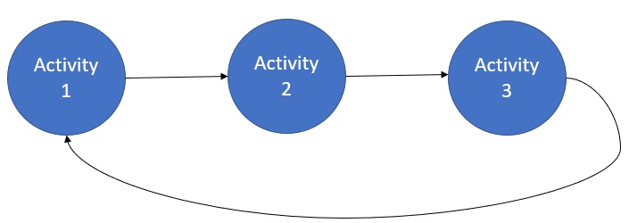
Figure 1. Simple Strictly Sequential Process

Suppose that according to the SMEs, for the activities of this process, we have exponentially distributed durations with means: $\beta_{1}=86$, $\beta_{2}=91$, and $\beta_{3}=163$. All these durations are in hours. The corresponding duration rate matrix is

$$\textbf{Q}=\begin{pmatrix}-1/86&1/86&0\\ 0&-1/91&1/91\\ 1/163&0&-1/163\end{pmatrix}.$$

If we observe emissions (e.g., resources in the field, or other observable objects) interrelated with the activities of this process every 20 hours, we can use the method in Section 4.2 to derive the transition probability matrices. Additionally, we assume there are four possible observation types $A$, $B$, $C$, and $D$ with a known emission probabilities resulting in the following transition and emission matrices

$$\textbf{T}(20)=\begin{pmatrix}0.793&0.185&0.021\\ 0.011&0.804&0.185\\ 0.103&0.012&0.885\end{pmatrix}\quad\textbf{E}=\begin{pmatrix}0.1&0.15&0.65&0.1\\ 0.05&0.1&0.5&0.35\\ 0.15&0.7&0.05&0.1\end{pmatrix}.$$

To evaluate the tensor factorization method we simulated the process model using Simian to evaluate the active processes at 20 hour intervals and apply the emission probabilities to the active processes for 1,000,000 runs. From the sequence of observed values the joint probability tensor and matrices were empirically evaluated and decomposed.

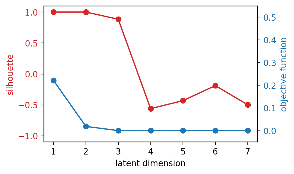
(a) Silhouette scores and objective function values for each candidate latent dimension.

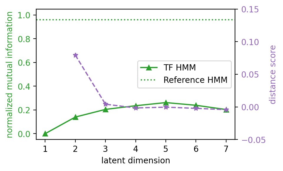
(b) Normalized mutual information and distance scores for each candidate latent dimension.

Figure 2. Tensor factorization parameter selection and evaluation for simple strictly sequential process.

Figure 2(a) shows the silhouette scores and objective function values for each candidate dimension. We see that our stability criteria clearly identifies $3$ hidden states for the HMM with a silhouette score close to 1.0 and objective value close to 0.0. The tensor emission and transition matrices are

$$\textbf{T}_{\text{tensor}}(20)=\begin{pmatrix}0.809&0.168&0.023\\ 0.011&0.787&0.202\\ 0.093&0.021&0.886\end{pmatrix}\quad\textbf{E}_{\text{tensor}}=\begin{pmatrix}0.098&0.149&0.641&0.113\\ 0.046&0.095&0.496&0.363\\ 0.15&0.7&0.05&0.099\end{pmatrix}.$$

The distance score in Figure 2(b) at each latent dimension indicates if their is an advantage of that latent dimension over the previous latent dimension. We see a large positive value at three, indicating it is advantageous over a latent dimension of two, and a value close to 0.0 at a latent dimension of four, indicating that a latent dimension of four is not significantly better than three. This aligns with the silhouette selection criteria. The normalized mutual information is relatively high at three, but peaks at a latent dimension of five. The correct selection of a latent dimension based on the silhouette and relative error demonstrates our ability to construct minimal HMMs from a theoretical process model with no parallelism.

4.2. Synthetic Example with Process Model Activities that do not Lead to Minimal HMM

Now suppose we consider another process that is similar to the previous process but now there is a fourth activity that runs concurrently with the third activity. This process is illustrated in Figure 3.

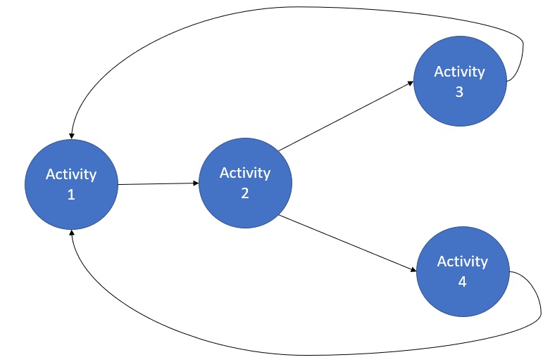
Figure 3. Simple Process with Parallel Activities

The mean duration for this fourth activity is $\beta_{4}=100$. The duration rate matrix is

$$\textbf{Q}=\begin{pmatrix}-1/86&1/86&0&0&0\\ 0&-1/91&1/91&0&0\\ 0&0&-1/163-1/100&1/163&1/100\\ 1/163&0&0&-1/163&0\\ 1/100&0&0&0&-1/100\end{pmatrix}$$

The transition probability matrix that we derive for this process is

$$\textbf{T}(20)=\begin{pmatrix}0.793&0.185&0.020&0.001&0.001\\ 0.001&0.803&0.168&0.011&0.017\\ 0.021&0.001&0.724&0.100&0.154\\ 0.103&0.011&0.001&0.885&0.000\\ 0.161&0.019&0.001&0.000&0.819\end{pmatrix}$$

Suppose also that the emission probability matrix that we assess from subject matter experts is

$$\textbf{E}=\begin{pmatrix}0.1&0.15&0.65&0.1\\ 0.05&0.1&0.5&0.35\\ 0.15&0.7&0.05&0.1\\ 0.15&0.7&0.05&0.1\\ 1&0&0&0\end{pmatrix}$$

For this process, the HMM we derive directly from the process is not minimal and we actually obtain a representation of the process with fewer parameters and states using the tensor factorization method. Our selection criteria identifies four instead of the reference five latent dimensions with a high silhouette score and low relative error in Figure 4(a).

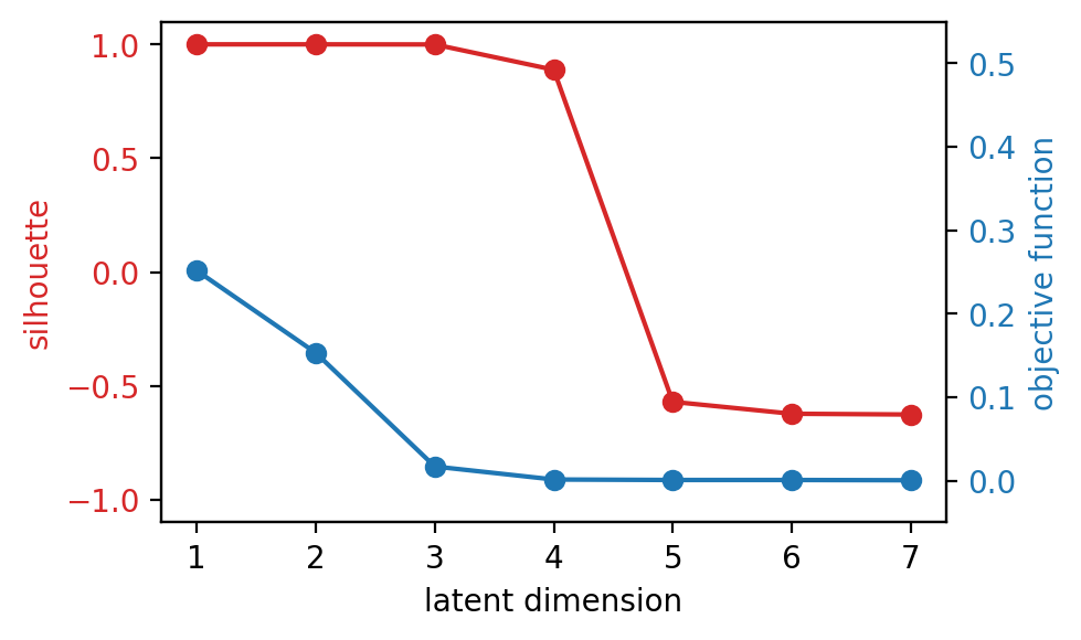
(a) Silhouette scores and objective function values for each candidate latent dimension.

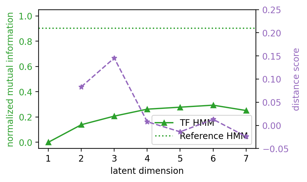
(b) Normalized mutual information and distance scores for each candidate latent dimension.

Figure 4. Tensor factorization parameter selection and evaluation for concurrent process.

$$\textbf{T}_{\text{tensor}}(20)=\begin{pmatrix}0.755&0.21&0.033&0.002\\ 0.05&0.739&0.2&0.011\\ 0.063&0.022&0.879&0.036\\ 0.147&0.026&0.008&0.82\end{pmatrix}\quad\textbf{E}_{\text{tensor}}=\begin{pmatrix}0.102&0.144&0.651&0.102\\ 0.042&0.093&0.495&0.37\\ 0.15&0.701&0.05&0.099\\ 0.994&0.003&0.001&0.002\end{pmatrix}.$$

The distance score in Figure 4(b) also suggests the latent dimension of four is the most suitable selection, since at four the distance score is slightly positive, and five it is negative. Interestingly the normalized mutual information continues to grow beyond four and peaks at six. By identifying a smaller HMM than the reference HMM, this validates that our selection criteria can find minimal HMMs of process models with parallelism.

4.3. Real Life Example: HMM of a Dutch Bank Loan Application Process Model

To illustrate our techniques, we looked at a set of event logs for a loan approval process for a bank in the Netherlands (for the bank data see (Moreira et al., 2018) and references therein). The data set contains event logs for 13,087 loan applications. Each event log contains the events (e.g., loan application acceptance, loan offer made, etc.) and activities (reviewing application, calling customer for information, etc.) that occurred while each loan was being processed, the associated time stamps for each of those events and activities, and the ids of the bank employees who completed each activity.

Next, we build a process model to describe this loan application process. The true loan application process is very complicated, since there are different paths a loan might take through the process (it might get accepted or rejected), it is possible to return to an activity previously completed, there are long time gaps (breaks, evenings, waiting for customer response, etc.) between activities and within activities, and there are activities that show up in some runs of the process but not others (sometimes an application is investigated for fraud, sometimes it is not). In order to simplify the modeling, we consider a simplified version of the loan application process. First, we only consider loans that made it to final approval (there are 2,246 such applications). Of these approved applications, we only consider applications that went through the following activities in the following order:

1. Afhandelen leads (Handling Leads)

2. Completeren aanvraag (Complete Application)

3. Nabellen offertes (Call customer about initial offer)

4. Valideren aanvraag (Validate/Assess Application) and Nabellen incomplete dossiers (Call customer about incomplete application information) completed concurrently

The first activity refers to bank agents determining whether the applicant is someone the bank already had a lead on. In the second activity, the bank employees ensure the completeness of the loan application, seek out additional information from the customer, and complete any parts of the application required on behalf of the bank. In the third activity, bank employees call the customers after they have received their initial loan offer to further discuss the offer with the customer. If the customer is not satisfied with the initial offer, they can ask the employees to reassess the application. While this reassessment is happening, employees may call the customer for additional information. This process is illustrated with a process model diagram in Figure 5. Of the 2,446 approved loans, 347 cases match this exact ordering of activities.

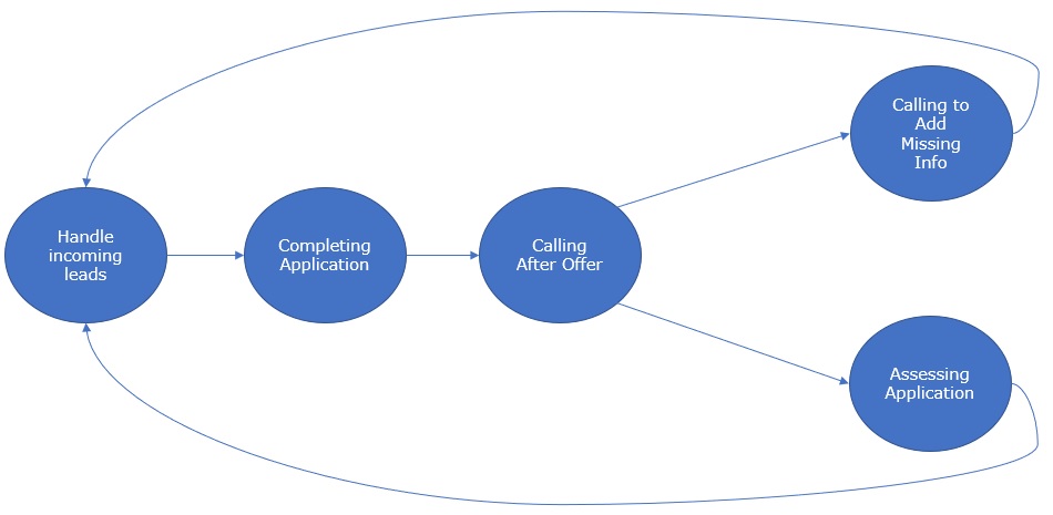
Figure 5. Loan Process Diagram

We further simplify the process by deleting the time gaps between and within activities. In the true process, there are long gaps between when an activity is finished and when the next one is started, we simplify this and assume that the activities happen one right after the other. In the true process, part of an activity is completed by one employee, then there is usually a time gap and then another part of the activity is completed by another employee. We eliminate this time gap between different parts of the same activity. The total duration spent in each activity is then the sum of the times between the start and end of each part of each activity. These simplifications are illustrated for sequential activities in Fig. 6.

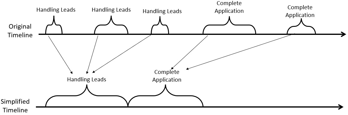
Figure 6. Removing Time Gaps Between and Within Sequential Activities.

For activities running in parallel, like the last two activities of this process, the simplification is a little more complex. We again take the total duration of each of the activities running in parallel to be the sum of the gaps between each start and end time, but we also determine when these activities would start relative to one another. In the true process there is a gap between the start of one activity and the start of the other activity that runs parallel with it. We simplify the model by assuming the activities start at the same time. The activity that finishes first is the one with shorter duration as determined previously. The simplification for parallel activities is depicted in Fig. 7.

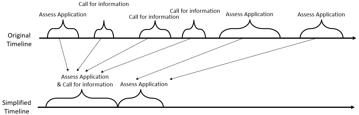
Figure 7. Removing Time Gaps Between and Within Concurrent Activities.

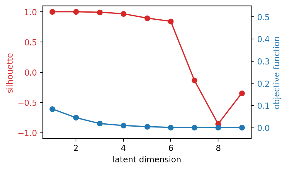
(a) Silhouette scores and objective function values for each candidate latent dimension.

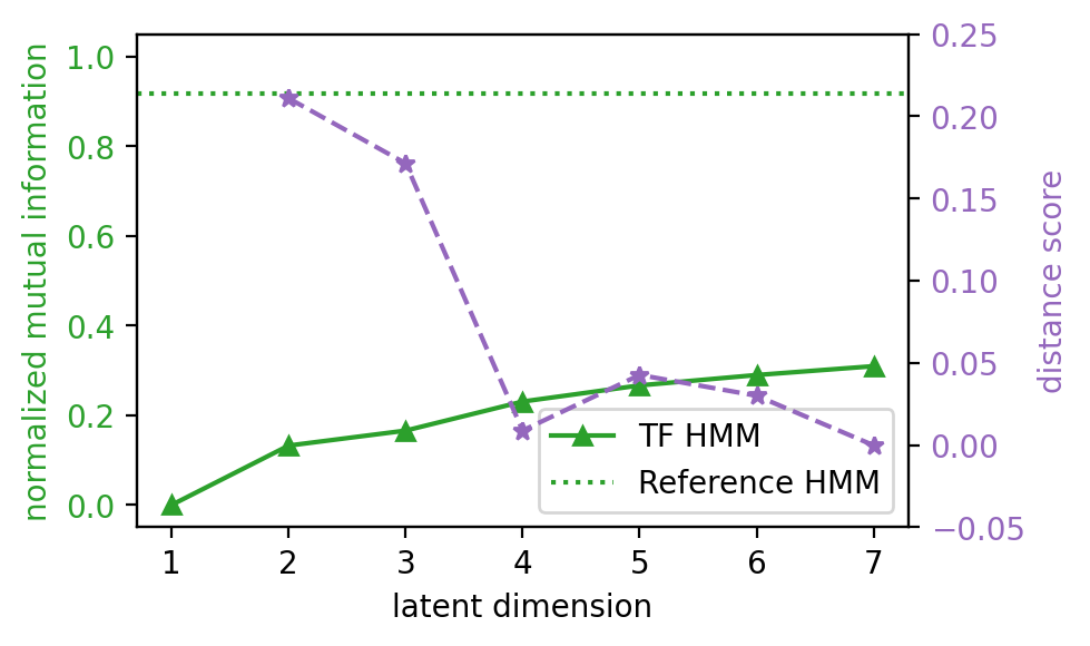
(b) Normalized mutual information and distance scores for each candidate latent dimension.

Figure 8. Tensor factorization parameter selection and evaluation for banking process model.

The silhouette scores and relative errors in Figure 8(a) clearly indicate six identifiable features, the same number of latent features as of the reference HMM. This agrees with the distance score analysis in Figure 8(b) with a positive value at six, and approximately zero at seven. The normalized mutual information is slightly greater at seven than six. The reference and tensor transition matrices are,

$$\textbf{T}(1/4)=\begin{pmatrix}0.578&0.323&0.084&0.013&0.001&0.001\\ 0.001&0.6&0.314&0.075&0.004&0.007\\ 0.004&0.001&0.629&0.301&0.024&0.041\\ 0.029&0.005&0.001&0.67&0.111&0.184\\ 0.103&0.027&0.004&0.001&0.865&0.0\\ 0.172&0.045&0.008&0.001&0.0&0.774\end{pmatrix}$$

$$\textbf{T}_{\text{tensor}}(1/4)=\begin{pmatrix}0.596&0.307&0.089&0.004&0.002&0.004\\ 0.002&0.597&0.31&0.005&0.031&0.054\\ 0.018&0.002&0.64&0.086&0.107&0.147\\ 0.139&0.04&0.03&0.285&0.377&0.129\\ 0.058&0.036&0.001&0.083&0.814&0.009\\ 0.071&0.06&0.003&0.055&0.074&0.737\end{pmatrix}\;.$$

The emission matrices for this example are not shown due to their significant number of observed states. The automatic selection of six identifiable features on this data demonstrates that our unsupervised selection criteria procedure constructs the right minimal HMMs on real data corresponding to a process model with parallelism.

5. Conclusion

Here we introduce a new unsupervised machine learning method based on non-negative tensor factorization for building minimal HMMs based on a theoretical process model constructed from domain expert estimations and implemented by Simian simulation engine (Santhi et al., 2015). Our new method is based on transfer of our technique for model selection in NMF and NTF, and gives us the opportunity to determine the unknown number of the hidden states in HMM as well to work with theoretical process models with sequential and parallel activities. The HMM built in this way allows us to answer questions of interest using domain expertise and scarce observational data.

Conflict of interest

The authors declare that they have no conflict of interest.

References

- (1)
- Agrawal et al. (1998) Rakesh Agrawal, Dimitrios Gunopulos, and Frank Leymann. 1998. Mining process models from workflow logs. In International Conference on Extending Database Technology. Springer, 467–483.
- Alexandrov et al. (2020) Boian S Alexandrov, Ludmil B Alexandrov, Filip L Iliev, Valentin G Stanev, and Velimir V Vesselinov. 2020. Source identification by non-negative matrix factorization combined with semi-supervised clustering. US Patent 10,776,718.
- Alexandrov and Rasmussen (2021) Boian S Alexandrov and Kim Orskov Rasmussen. 2021. SmartTensors AI Platform. Los Alamos National Laboratory Technical Report, LA-UR-21-25064.
- Alexandrov et al. (2019) Boian S Alexandrov, Valentin G Stanev, Velimir V Vesselinov, and Kim Ø Rasmussen. 2019. Nonnegative tensor decomposition with custom clustering for microphase separation of block copolymers. Statistical Analysis and Data Mining: The ASA Data Science Journal 12, 4 (2019), 302–310.
- Alharbi (2019) Amirah Mohammed Alharbi. 2019. Unsupervised abstraction for reducing the complexity of healthcare process models. Ph. D. Dissertation. University of Leeds.
- Allman et al. (2009) Elizabeth S Allman, Catherine Matias, and John A Rhodes. 2009. Identifiability of parameters in latent structure models with many observed variables. The Annals of Statistics 37, 6A (2009), 3099–3132.
- Apostolico and Bejerano (2000) Alberto Apostolico and Gill Bejerano. 2000. Optimal amnesic probabilistic automata or how to learn and classify proteins in linear time and space. Journal of Computational Biology 7, 3-4 (2000), 381–393.
- Baum et al. (1970) Leonard E Baum, Ted Petrie, George Soules, and Norman Weiss. 1970. A maximization technique occurring in the statistical analysis of probabilistic functions of Markov chains. The annals of mathematical statistics 41, 1 (1970), 164–171.
- Brand (1998) Matthew Brand. 1998. An entropic estimator for structure discovery. Advances in Neural Information Processing Systems 11 (1998).
- Carrera and Jung (2014) Berny Carrera and Jae-Yoon Jung. 2014. Constructing probabilistic process models based on hidden markov models for resource allocation. In International Conference on Business Process Management. Springer, 477–488.
- Cohen (1998) A Cohen. 1998. Hidden Markov models in biomedical signal processing. In Proceedings of the 20th Annual International Conference of the IEEE Engineering in Medicine and Biology Society. Vol. 20 Biomedical Engineering Towards the Year 2000 and Beyond (Cat. No. 98CH36286), Vol. 3. IEEE, 1145–1150.
- Cybenko and Crespi (2011) George Cybenko and Valentino Crespi. 2011. Learning hidden Markov models using nonnegative matrix factorization. IEEE Transactions on Information Theory 57, 6 (2011), 3963–3970.
- Da Silva and Ferreira (2009) Gil Aires Da Silva and Diogo R Ferreira. 2009. Applying hidden Markov models to process mining. Sistemas e Tecnologias de Informação. AISTI/FEUP/UPF (2009).
- Higham (2005) Nicholas J Higham. 2005. The Scaling and Squaring Method for the Matrix Exponential Revisited. SIAM J. Matrix Anal. Appl. 26, 4 (2005), 1179–1193.
- Huang et al. (2018) Kejun Huang, Xiao Fu, and Nicholas Sidiropoulos. 2018. Learning hidden Markov models from pairwise co-occurrences with application to topic modeling. In International Conference on Machine Learning. PMLR, 2068–2077.
- Huang et al. (2015) Qingqing Huang, Rong Ge, Sham Kakade, and Munther Dahleh. 2015. Minimal realization problems for hidden markov models. IEEE Transactions on Signal Processing 64, 7 (2015), 1896–1904.
- Jaramillo and Arias (2019) Johnnatan Jaramillo and Julián Arias. 2019. Automatic classification of event logs sequences for failure detection in WfM/BPM systems. In 2019 IEEE Colombian Conference on Applications in Computational Intelligence (ColCACI). IEEE, 1–6.
- Kalenkova et al. (2022) Anna Kalenkova, Lewis Mitchell, and Matthew Roughan. 2022. Performance Analysis: Discovering Semi-Markov Models From Event Logs. arXiv preprint arXiv:2206.14415 (2022).
- Khatri and Rao (1968) CG Khatri and C Radhakrishna Rao. 1968. Solutions to some functional equations and their applications to characterization of probability distributions. Sankhyā: The Indian Journal of Statistics, Series A (1968), 167–180.
- Kruskal (1977) Joseph B Kruskal. 1977. Three-way arrays: rank and uniqueness of trilinear decompositions, with application to arithmetic complexity and statistics. Linear algebra and its applications 18, 2 (1977), 95–138.
- Million (2007) Elizabeth Million. 2007. The hadamard product. Course Notes 3, 6 (2007).
- Moler and Van Loan (2003) Cleve Moler and Charles Van Loan. 2003. Nineteen Dubious Ways to Compute the Exponential of a Matrix, Twenty-five Years Later. SIAM review 45, 1 (2003), 3–49.
- Moreira et al. (2018) Catarina Moreira, Emmanuel Haven, Sandro Sozzo, and Andreas Wichert. 2018. Process mining with real world financial loan applications: Improving inference on incomplete event logs. PLoS One 13, 12 (2018), e0207806.
- Nebgen et al. (2021) Benjamin T Nebgen, Raviteja Vangara, Miguel A Hombrados-Herrera, Svetlana Kuksova, and Boian S Alexandrov. 2021. A neural network for determination of latent dimensionality in non-negative matrix factorization. Machine Learning: Science and Technology 2, 2 (2021), 025012.
- Ohta (2021) Yoshito Ohta. 2021. On the Realization of Hidden Markov Models and Tensor Decomposition. IFAC-PapersOnLine 54, 9 (2021), 725–730.
- Perronnin et al. (2005) Florent Perronnin, J-L Dugelay, and Kenneth Rose. 2005. A probabilistic model of face mapping with local transformations and its application to person recognition. IEEE transactions on pattern analysis and machine intelligence 27, 7 (2005), 1157–1171.
- Rabiner and Juang (1986) Lawrence Rabiner and Biinghwang Juang. 1986. An introduction to hidden Markov models. ieee assp magazine 3, 1 (1986), 4–16.
- Rabiner (1989) Lawrence R Rabiner. 1989. A tutorial on hidden Markov models and selected applications in speech recognition. Proc. IEEE 77, 2 (1989), 257–286.
- Rahmawati et al. (2017) Dewi Rahmawati, Riyanarto Sarno, Chastine Fatichah, and Dwi Sunaryono. 2017. Fraud detection on event log of bank financial credit business process using Hidden Markov Model algorithm. In 2017 3rd International Conference on Science in Information Technology (ICSITech). IEEE, 35–40.
- Ross (1996) Sheldon M Ross. 1996. Stochastic Processes. Vol. 2. Wiley New York.
- Rousseeuw (1987) Peter J Rousseeuw. 1987. Silhouettes: a graphical aid to the interpretation and validation of cluster analysis. Journal of computational and applied mathematics 20 (1987), 53–65.
- Santhi et al. (2015) Nandakishore Santhi, Stephan Eidenbenz, and Jason Liu. 2015. The simian concept: Parallel discrete event simulation with interpreted languages and just-in-time compilation. In 2015 Winter Simulation Conference (WSC). IEEE, 3013–3024.
- Sarno and Sungkono (2016) Riyanarto Sarno and Kelly R Sungkono. 2016. Hidden markov model for process mining of parallel business processes. International Review on Computers and Software (IRECOS) 11, 4 (2016), 290–300.
- Sastre et al. (2015) Jorge Sastre, J Ibáñez, Emilio Defez, and P Ruiz. 2015. New scaling-squaring Taylor algorithms for computing the matrix exponential. SIAM Journal on Scientific Computing 37, 1 (2015), A439–A455.
- Schruben and Yücesan (1993) Lee Schruben and Enver Yücesan. 1993. Modeling paradigms for discrete event simulation. Operations Research Letters 13, 5 (1993), 265–275.
- Song et al. (2001) Dawn Xiaodong Song, David Wagner, and Xuqing Tian. 2001. Timing Analysis of Keystrokes and Timing Attacks on SSH. In 10th USENIX Security Symposium (USENIX Security 01).
- Tune et al. (2013) Paul Tune, Hung X Nguyen, and Matthew Roughan. 2013. Hidden Markov model identifiability via tensors. In 2013 IEEE International Symposium on Information Theory. IEEE, 2299–2303.
- Van Der Aalst et al. (2007) Wil MP Van Der Aalst, Hajo A Reijers, Anton JMM Weijters, Boudewijn F van Dongen, AK Alves De Medeiros, Minseok Song, and HMW Verbeek. 2007. Business process mining: An industrial application. Information Systems 32, 5 (2007), 713–732.
- Vangara et al. (2020) Raviteja Vangara, Erik Skau, Gopinath Chennupati, Hristo Djidjev, Thomas Tierney, James P Smith, Manish Bhattarai, Valentin G Stanev, and Boian S Alexandrov. 2020. Semantic nonnegative matrix factorization with automatic model determination for topic modeling. In 2020 19th IEEE International Conference on Machine Learning and Applications (ICMLA). IEEE, 328–335.
- Vaseghi (2008) Saeed V Vaseghi. 2008. Advanced digital signal processing and noise reduction. John Wiley & Sons.
- Viterbi (1967) Andrew Viterbi. 1967. Error bounds for convolutional codes and an asymptotically optimum decoding algorithm. IEEE transactions on Information Theory 13, 2 (1967), 260–269.
- Yang et al. (2020) Lingkai Yang, Sally McClean, Mark Donnelly, Kashaf Khan, and Kevin Burke. 2020. Analysing Business Process Anomalies Using Discrete-time Markov chains. In 2020 IEEE 22nd International Conference on High Performance Computing and Communications; IEEE 18th International Conference on Smart City; IEEE 6th International Conference on Data Science and Systems (HPCC/SmartCity/DSS). IEEE, 1258–1265.