Expediting Large-Scale Vision Transformer
for Dense Prediction without Fine-tuning

Abstract

Vision transformers have recently achieved competitive results across various vision tasks but still suffer from heavy computation costs when processing a large number of tokens. Many advanced approaches have been developed to reduce the total number of tokens in large-scale vision transformers, especially for image classification tasks. Typically, they select a small group of essential tokens according to their relevance with the [class] token, then fine-tune the weights of the vision transformer. Such fine-tuning is less practical for dense prediction due to the much heavier computation and GPU memory cost than image classification.

In this paper, we focus on a more challenging problem, i.e., accelerating large-scale vision transformers for dense prediction without any additional re-training or fine-tuning. In response to the fact that high-resolution representations are necessary for dense prediction, we present two non-parametric operators, a token clustering layer to decrease the number of tokens and a token reconstruction layer to increase the number of tokens. The following steps are performed to achieve this: (i) we use the token clustering layer to cluster the neighboring tokens together, resulting in low-resolution representations that maintain the spatial structures; (ii) we apply the following transformer layers only to these low-resolution representations or clustered tokens; and (iii) we use the token reconstruction layer to re-create the high-resolution representations from the refined low-resolution representations. The results obtained by our method are promising on five dense prediction tasks, including object detection, semantic segmentation, panoptic segmentation, instance segmentation, and depth estimation. Accordingly, our method accelerates $40\%\uparrow$ FPS and saves $30\%\downarrow$ GFLOPs of “Segmenter+ViT-L/$16$” while maintaining $99.5\%$ of the performance on ADE$20$K without fine-tuning the official weights.

1 Introduction

Transformer [67] has made significant progress across various challenging vision tasks since pioneering efforts such as DETR [4], Vision Transformer (ViT) [18], and Swin Transformer [47]. By removing the local inductive bias [19] from convolutional neural networks [28, 64, 60], vision transformers armed with global self-attention show superiority in scalability for large-scale models and billion-scale dataset [18, 84, 61], self-supervised learning [27, 76, 1], connecting vision and language [53, 34], etc. We can find from recent developments of SOTA approaches that vision transformers have dominated various leader-boards, including but not limited to image classification [74, 14, 17, 84], object detection [86, 46, 38], semantic segmentation [32, 11, 3], pose estimation [77], image generation [85], and depth estimation [42].

Although vision transformers have achieved more accurate predictions in many vision tasks, large-scale vision transformers are still burdened with heavy computational overhead, particularly when processing high-resolution inputs [20, 46], thus limiting their broader application to more resource-constrained applications and attracting efforts on re-designing light-weight vision transformer architectures [10, 51, 87]. In addition to this, several recent efforts have investigated how to decrease the model complexity and accelerate vision transformers, especially for image classification, and introduced various advanced approaches to accelerate vision transformers. Dynamic ViT [55] and EViT [44], for example, propose two different dynamic token sparsification frameworks to reduce the redundant tokens progressively and select the most informative tokens according to the scores predicted with an extra trained prediction module or their relevance with the [class] token. TokenLearner [58] learns to spatially attend over a subset of tokens and generates a set of clustered tokens adaptive to the input for video understanding tasks. Most of these token reduction approaches are carefully designed for image classification tasks and require fine-tuning or retraining. These approaches might not be suitable to tackle more challenging dense prediction tasks that need to process high-resolution input images, e.g., $1024\times 1024$, thus, resulting in heavy computation and GPU memory cost brought. We also demonstrate in the supplemental material the superiority of our method over several representative methods on dense prediction tasks.

Rather than proposing a new lightweight architecture for dense prediction or token reduction scheme for only image classification, we focus on how to expedite well-trained large-scale vision transformers and use them for various dense prediction tasks without fine-tuning or re-training. Motivated by these two key observations including (i) the intermediate token representations of a well-trained vision transformer carry a heavy amount of local spatial redundancy and (ii) dense prediction tasks require high-resolution representations, we propose a simple yet effective scheme to convert the “high-resolution” path of the vision transformer to a “high-to-low-to-high resolution” path via two non-parametric layers including a token clustering layer and a token reconstruction layer. Our method can produce a wide range of more efficient models without requiring further fine-tuning or re-training. We apply our approach to expedite two main-stream vision transformer architectures, e.g., ViTs and Swin Transformers, for five challenging dense prediction tasks, including object detection, semantic segmentation, panoptic segmentation, instance segmentation, and depth estimation. We have achieved encouraging results across several evaluated benchmarks and Figure 1 illustrates some representative results on both semantic segmentation and depth estimation tasks.

2 Related work

Pruning Convolutional Neural Networks.

Convolutional neural network pruning [2, 30, 71] is a task that involves removing the redundant parameters to reduce the model complexity without a significant performance drop. Pruning methods typically entail three steps: (i) training a large, over-parameterized model to convergence, (ii) pruning the trained large model according to a certain criterion, and (iii) fine-tuning the pruned model to regain the lost performance [49]. The key idea is to design an importance score function that is capable of pruning the less informative parameters. We follow [7] to categorize the existing methods into two main paths: (i) unstructured pruning (also named weight pruning) and (ii) structured pruning. Unstructured pruning methods explore the absolute value of each weight or the product of each weight and its gradient to estimate the importance scores. Structured pruning methods, such as layer-level pruning [72], filter-level pruning[48, 79], and image-level pruning [25, 65], removes the model sub-structures. Recent studies [5, 6, 31] further extend these pruning methods to vision transformer. Unlike the previous pruning methods, we explore how to expedite vision transformers for dense prediction tasks by carefully reducing & increasing the number of tokens without removing or modifying the parameters.

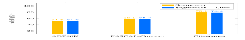
(a) mIoU@Segmenter

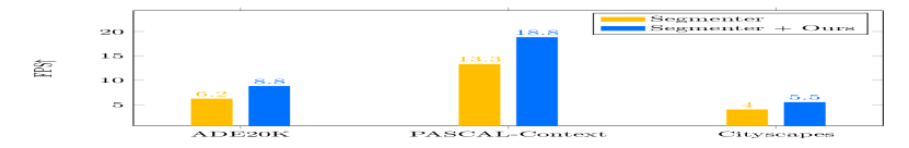
(b) FPS@Segmenter

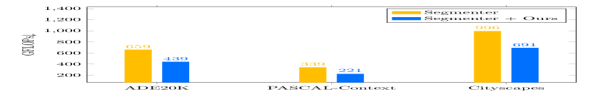
(c) GFLOPs@Segmenter

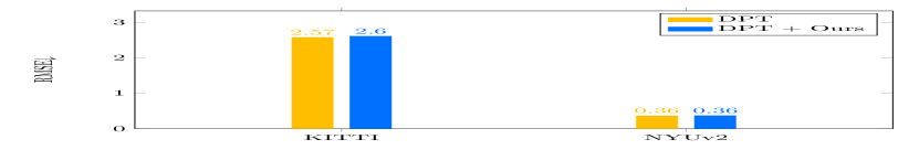
(d) RMSE@DPT

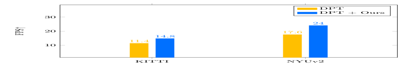
(e) FPS@DPT

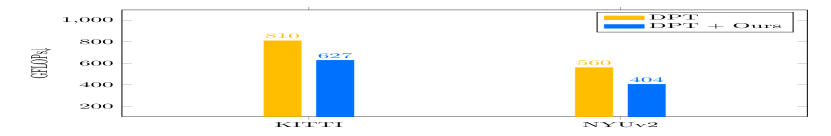
(f) GFLOPs@DPT

Figure 1: Illustrating the improvements of our approach: we report the results of applying our approach to Segmenter [63] for semantic segmentation and DPT [54] for depth estimation on the $1$-st and $2$-ed row respectively. Without any fine-tuning, our proposed method reduces the GFLOPs and accelerates the FPS significantly with a slight performance drop on both dense prediction tasks. $\uparrow$ and $\downarrow$ represent higher is better and lower is better respectively. Refer to Section 4 for more details.

Efficient Vision Transformer.

The success of vision transformers has incentivised many recent efforts [58, 62, 50, 29, 73, 55, 37, 24, 69, 9, 35, 44, 57] to exploit the spatial redundancies of intermediate token representations. For example, TokenLearner [58] learns to attend over a subset of tokens and generates a set of clustered tokens adaptive to the input. They empirically show that very few clustered tokens are sufficient for video understanding tasks. Token Pooling [50] exploits a nonuniform data-aware down-sampling operator based on K-Means or K-medoids to cluster similar tokens together to reduce the number of tokens while minimizing the reconstruction error. Dynamic ViT [55] observes that the accurate image recognition with vision transformers mainly depends on a subset of the most informative tokens, and hence it develops a dynamic token sparsification framework for pruning the redundant tokens dynamically based on the input. EViT (expediting vision transformers) [44] proposes to calculate the attentiveness of the [class] token with respect to each token and identify the top-$k$ attentive tokens according to the attentiveness score. Patch Merger [56] uses a learnable attention matrix to merge and combine together the redundant tokens, therefore creating a much more practical and cheaper model with only a slight performance drop. Refer to [66] for more details on efficient transformer architecture designs, such as Performer [12] and Reformer [36]. In contrast to these methods that require either retraining or fine-tuning the modified transformer architectures from scratch or the pre-trained weights, our approach can reuse the once-trained weights for free and produce lightweight models with a modest performance drop.

Vision Transformer for Dense Prediction.

In the wake of success of the representative pyramid vision transformers [47, 70] for object detection and semantic segmentation, more and more efforts have explored different advanced vision transformer architecture designs [39, 8, 40, 41, 21, 81, 78, 88, 23, 43, 75, 80, 16, 83, 82, 26] suitable for various dense prediction tasks. For example, MViT [40] focuses more on multi-scale representation learning, while HRFormer [81] examines the benefits of combining multi-scale representation learning and high-resolution representation learning. Instead of designing a novel vision transformer architecture for dense prediction, we focus on how to accelerate a well-trained vision transformer while maintaining the prediction performance as much as possible.

Our approach.

The contribution of our work lies in two main aspects: (i) we are the first to study how to accelerate state-of-the-art large-scale vision transformers for dense prediction tasks without fine-tuning (e.g., "Mask2Former + Swin-L" and "SwinV2-L + HTC++"). Besides, our approach also achieves much better accuracy and speedup trade-off when compared to the very recent ACT [1] which is based on a clustering attention scheme; (ii) our token clustering and reconstruction layers are capable of maintaining the semantic information encoded in the original high-resolution representations. This is the very most important factor to avoid fine-tuning. We design an effective combination of a token clustering function and a token reconstruction function to maximize the cosine similarity between the reconstructed high-resolution feature maps and the original ones without fine-tuning. The design of our token reconstruction layer is the key and not straightforward essentially. We also show that our token reconstruction layer can be used to adapt the very recent EViT [44] and DynamicViT [55] for dense prediction tasks in the supplementary.

3 Our Approach

(a)

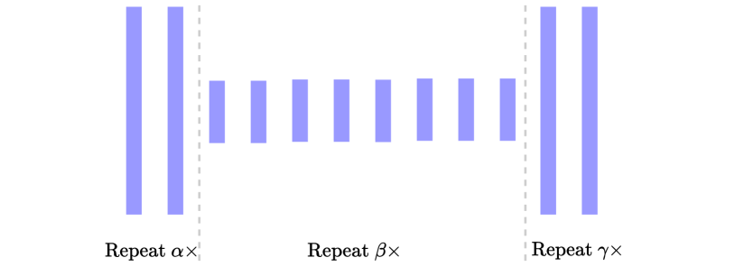
(b)

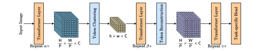
(c)

Figure 2: (a) Plain high-resolution vision transformer with $\mathsf{L}$ layers. (b) U-shape High-to-low-to-high-resolution vision transformer with $\alpha$, $\beta$, and $\gamma$ layers respectively ($\mathsf{L}=\alpha+\beta+\gamma$). (c) Illustrating the details of using our approach to plain ViTs: we insert a token clustering layer and a token reconstruction layer into a trained vision transformer in order to decrease and then increase the spatial resolution, respectively. The weights of modules marked with   are trained once based on the configuration of (a). The token clustering layer and token reconstruction layer are marked with   are non-parametric, thus do not require any fine-tuning and can be included directly during evaluation.

Preliminary. The conventional Vision Transformer [18] first reshapes the input image $\mathbf{X}\in\mathbb{R}^{\mathsf{H}\times\mathsf{W}\times\mathsf{3}}$ into a sequence of flatten patches $\mathbf{X}_{p}\in\mathbb{R}^{\mathsf{N}\times(\mathsf{P}^{2}\mathsf{3})}$, where $(\mathsf{P},\mathsf{P})$ represents the resolution of each patch, $(\mathsf{H},\mathsf{W})$ represents the resolution of the input image, $\mathsf{N}=(\mathsf{H}\times\mathsf{W})/{\mathsf{P}^{2}}$ represents the number of resulting patches or tokens, i.e., the input sequence length. The Vision Transformer consists of alternating layers of multi-head self-attention ($\operatorname{MHSA}$) and feed-forward network ($\operatorname{FFN}$) accompanied with layer norm ($\operatorname{LN}$) and residual connections:

$${\mathbf{Z}_{l}^{{}^{\prime}}} =\operatorname{MHSA}\left(\mathrm{LN}\left(\mathbf{Z}_{l-1}\right)\right)+\mathbf{Z}_{l-1},$$ (1)

$${\mathbf{Z}_{l}} =\operatorname{FFN}\left(\mathrm{LN}\left({\mathbf{Z}_{l}^{{}^{\prime}}}\right)\right)+{\mathbf{Z}_{l}^{{}^{\prime}}},$$

where $l\in\{1,\dots,\mathsf{L}\}$ represents the layer index, $\mathbf{Z}_{l}\in\mathbb{R}^{\mathsf{N}\times\mathsf{C}}$, and $\mathbf{Z}_{0}$ is based on $\mathbf{X}_{p}$. The computation cost $\mathcal{O}(\mathsf{L}\mathsf{N}\mathsf{C}(\mathsf{N}+\mathsf{C}))$ mainly depends on the number of layers $\mathsf{L}$, the number of tokens $\mathsf{N}$, and the channel dimension $\mathsf{C}$.

Despite the great success of transformer, its computation cost increases significantly when handling high-resolution representations, which are critical for dense prediction tasks. This paper attempts to resolve this issue by reducing the computation complexity during the inference stage, and presents a very simple solution for generating a large number of efficient vision transformer models directly from a single trained vision transformer, requiring no further training or fine-tuning.

We demonstrate how our approach could be applied to the existing standard Vision Transformer in Figure 2. The original Vision Transformer is modified using two non-parametric operations, namely a token clustering layer and a token reconstruction layer. The proposed token clustering layer is utilized to convert the high-resolution representations to low-resolution representations by clustering the locally semantically similar tokens. Then, we apply the following transformer layers on the low-resolution representations, which greatly accelerates the inference speed and saves computation resources. Last, a token reconstruction layer is proposed to reconstruct the feature representations back to high-resolution.

Token Clustering Layer. We construct the token clustering layer following the improved SLIC scheme [33], which performs local k-means clustering as follows:

-Initial superpixel center: We apply adaptive average pooling ($\operatorname{AAP}$) over the high-resolution representations from the $\alpha$-th layer to compute the $\mathsf{h}\times\mathsf{w}$ initial cluster center representations:

$$\mathbf{S}_{\alpha}=\operatorname{AAP}(\mathbf{Z}_{\alpha},(\mathsf{h}\times\mathsf{w})),$$ (2)

where $\mathbf{S}_{\alpha}\in\mathbb{R}^{\mathsf{hw}\times\mathsf{C}}$, $\mathbf{Z}_{\alpha}\in\mathbb{R}^{\mathsf{N}\times\mathsf{C}}$, and $\mathsf{hw}\ll\mathsf{N}$.

-Iterative local clustering: (i) Expectation step: compute the normalized similarity between each pixel $p$ and the surrounding superpixel $i$ (we only consider the neighboring $\lambda$ positions), (ii) Maximization step: compute the new superpixel centers:

$${\mathbf{Q}_{p,i}}=\frac{\rm{exp}\Big{(}\scalebox{0.75}[1.0]{$-$}||\mathbf{Z}_{\alpha,p}-\mathbf{S}_{\alpha,i}||^{2}/{\tau}\Big{)}}{\sum_{j=1}^{\lambda}\rm{exp}\Big{(}\scalebox{0.75}[1.0]{$-$}||\mathbf{Z}_{\alpha,p}-\mathbf{S}_{\alpha,j}||^{2}/{\tau}\Big{)}},\quad\mathbf{S}_{\alpha,i}=\sum_{p=1}^{\mathsf{N}}\mathbf{Q}_{p,i}\mathbf{Z}_{\alpha,p},$$ (3)

where we iterate the above Expectation step and Maximization step for $\kappa$ times, $\tau$ is a temperature hyper-parameter, and $i\in\{1,2,\cdots,\lambda\}$. We apply the following $\beta$ transformer layers on $\mathbf{S}_{\alpha}$ instead of $\mathbf{Z}_{\alpha}$, thus results in $\mathbf{S}_{\alpha+\beta}$ and decreases the computation cost significantly.

Token Reconstruction Layer. We implement the token reconstruction layer by exploiting the relations between the high-resolution representations and the low-resolution clustered representations:

$$\mathbf{Z}_{\alpha+\beta,p}=\sum_{\mathbf{S}_{\alpha,i}\in\textrm{k-NN}(\mathbf{Z}_{\alpha,p})}\frac{\textrm{exp}\big{(}\scalebox{0.75}[1.0]{$-$}{||\mathbf{Z}_{\alpha,p}-\mathbf{S}_{\alpha,i}||^{2}}/{\tau}\big{)}}{\sum_{\mathbf{S}_{\alpha,j}\in\textrm{k-NN}(\mathbf{Z}_{\alpha,p})}\textrm{exp}\big{(}\scalebox{0.75}[1.0]{$-$}||\mathbf{Z}_{\alpha,p}-\mathbf{S}_{\alpha,j}||^{2}/{\tau}\big{)}}\mathbf{S}_{\alpha+\beta,i},$$ (4)

where $\tau$ is the same temperature hyper-parameter as in Equation 3. $\textrm{k-NN}(\mathbf{Z}_{\alpha,p})$ represents a set of the k nearest, a.k.a, most similar, superpixel representations for $\mathbf{Z}_{\alpha,i}$. We empirically find that choosing the same neighboring positions as in Equation 3 achieves close performance as the k-NN scheme while being more easy to implementation.

In summary, we estimate their semantic relations based on the representations before refinement with the following $\beta$ transformer layers and then reconstruct the high-resolution representations from the refined low-resolution clustered representations accordingly.

Finally, we apply the remained $\gamma$ transformer layers to the reconstructed high-resolution features and the task-specific head on the refined high-resolution features to predict the target results such as semantic segmentation maps or monocular depth maps.

Extension to Swin Transformer. We further introduce the window token clustering layer and window token reconstruction layer, which are suitable for Swin Transformer [46, 47]. Figure 3 illustrates an example usage of the proposed window token clustering layer and window token reconstruction layer. We first cluster the $\mathsf{K}\times\mathsf{K}$ window tokens into $\mathsf{k}\times\mathsf{k}$ window tokens and then reconstruct $\mathsf{K}\times\mathsf{K}$ window tokens according to the refined $\mathsf{k}\times\mathsf{k}$ window tokens. We apply the swin transformer layer equipped with smaller window size $\mathsf{k}\times\mathsf{k}$ on the clustered representations, where we need to bi-linear interpolate the pre-trained weights of relative position embedding table from $(2\mathsf{K}-1)$$\times$$(2\mathsf{K}-1)$ to $(2\mathsf{k}-1)$$\times$$(2\mathsf{k}-1)$ when processing the clustered representations. In summary, we can improve the efficiency of Swin Transformer by injecting the window token clustering layer and the window token reconstruction layer into the backbones seamlessly without fine-tuning the model weights.

Why our approach can avoid fine-tuning? The reasons include the following two aspects: (i) our token clustering/reconstruction layers are non-parametric, thus avoiding retraining any additional parameters, (ii) the reconstructed high-resolution representations maintain high semantic similarity with the original high-resolution representations. We take Segmenter+ViT-L/$16$ (on ADEK, $\alpha$=$10$) as an example and analyze the semantic similarity between the reconstructed high-resolution feature (with our approach) and the original high-resolution feature (with the original ViT-L/$16$) in Table 1. Accordingly, we can see that the cosine similarities are consistently high across different transformer layers between the reconstructed high-resolution feature (with our approach) and the original high-resolution feature. In other words, our approach well maintains the semantic information carried in the original high-resolution feature maps and thus is capable of avoiding fine-tuning.

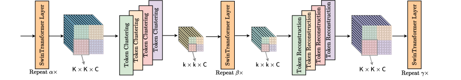
Figure 3: Illustrating the details of using our approach for Swin Transformer [46, 47]: we apply four groups of token clustering layer and token reconstruction layer within the four non-overlapped windows marked with  ,  ,  , and   respectively, in the example referred to as window token clustering layer and window token reconstruction layer. We apply the intermediate swin transformer layers equipped with window size $\mathsf{k}\times\mathsf{k}$) on the clustered window tokens. Window sizes before and after token clustering layer are $\mathsf{K}\times\mathsf{K}$ and $\mathsf{k}\times\mathsf{k}$, and vice versa, for the token reconstruction layer.

Table 1: Ablation of the cosine similarity between the reconstructed high-resolution feature maps and the original high-resolution feature maps, where $\mathbf{Z}_{\alpha+\beta}^{\rm{original}}$ and $\mathbf{Z}_{\alpha+\beta}$ represents the original and reconstructed high-resolution feature maps, respectively.

$\alpha$+$\beta$	$12$	$14$	$16$	$18$	$20$	$22$	$24$
cos($\mathbf{Z}_{\alpha+\beta}$, $\mathbf{Z}_{\alpha+\beta}^{\rm{original}}$)	$0.94$	$0.95$	$0.96$	$0.96$	$0.96$	$0.96$	$0.96$

4 Experiment

We verify the effectiveness of our method across five challenging dense prediction tasks, including object detection, semantic segmentation, instance segmentation, panoptic segmentation, and monocular depth estimation. We carefully choose the advanced SOTA methods that build the framework based on either the plain ViTs [18] or the Swin Transformers [46, 47]. We can integrate the proposed token clustering layer and token reconstruction layer seamlessly with the provided official trained checkpoints with no further fine-tuning required. More experimental details are illustrated as follows.

4.1 Datasets

COCO [45]. This dataset consists of $123$K images with $896$K annotated bounding boxes belonging to $80$ thing classes and $53$ stuff classes, where the train set contains $118$K images and the val set contains $5$K images. We report the object detection performance of SwinV2 + HTC++ [46] and the instance/panoptic segmentation performance of Mask$2$Former [11] on the val set.

ADE$20$K [90]. This dataset contains challenging scenes with fine-grained labels and is one of the most challenging semantic segmentation datasets. The train set contains $20,210$ images with $150$ semantic classes. The val set contains $2,000$ images. We report the segmentation results with Segmenter [63] on the val set.

PASCAL-Context [52]. This dataset consists of $59$ semantic classes plus a background class, where the train set contains $4,996$ images with and the val set contains $5,104$ images. We report the segmentation results with Segmenter [63] on the val set.

Cityscapes [13]. This dataset is an urban scene understanding dataset with $30$ classes while only $19$ classes are used for parsing evaluation. The train set and val set contains $2,975$ and $500$ images respectively. We report the segmentation results with Segmenter [63] on the val set.

KITTI [22]. This dataset provides stereo, optical flow, visual odometry (SLAM), and 3D object detection of outdoor scenes captured by equipment mounted on a moving vehicle. We choose DPT [54] as our baseline to conduct experiments on the monocular depth prediction tasks, which consists of around $26$K images for train set and $698$ images for val set, where only $653$ images have the ground-truth depth maps and the image resolution is of $1,241\times 376$.

NYUv$2$ [59]. This dataset consists of $1,449$ RGBD images with resolution of $640\times 480$, which captures $464$ diverse indoor scenes and contains rich detailed dense annotations such as surface normals, segmentation maps, depth, 3D planes, and so on. We report the depth prediction results of DPT [54] evaluated on $655$ val images.

4.2 Evaluation Metrics

We report the numbers of AP (average precision), mask AP (mask average precision), PQ (panoptic quality), mIoU (mean intersection-over-union), and RMSE (root mean squared error) across object detection, instance segmentation, panoptic segmentation, semantic segmentation, and depth estimation tasks respectively. Since the dense prediction tasks care less about the throughput used in image classification tasks [44], we report FPS to measure the latency and the number of GFLOPs to measure the model complexity during evaluation. FPS is tested on a single V100 GPU with Pytorch 1.10 and CUDA 10.2 by default. More details are provided in the supplementary material.

Table 2: Influence of the hyper-parameters of token clustering/reconstruction layer.

Parameter	$\lambda$			$\kappa$				$\tau$				$\mathrm{k}$
	$3\times 3$	$5\times 5$	$7\times 7$	$5$	$10$	$15$	$20$	$10$	$25$	$50$	$75$	$10$	$20$	$50$
GFLOPs	$438.6$	$438.9$	$439.6$	$438.9$	$439.6$	$440.2$	$440.8$	$438.9$				$438.9$	$438.9$	$439.0$
mIoU	$51.46$	$51.56$	$51.55$	$51.56$	$51.59$	$51.62$	$51.62$	$51.18$	$51.35$	$51.56$	$51.07$	$51.34$	$51.56$	$51.56$

Table 3: Influence of the cluster size $\mathsf{h}\times\mathsf{w}$.

Cluster size	$8\times 8$	$12\times 12$	$16\times 16$	$20\times 20$	$24\times 24$	$28\times 28$	$40\times 40$ (baseline)
GFLOPs	$274.0$	$290.9$	$315.1$	$347.2$	$388.2$	$438.9$	$659.0$
mIoU	$32.13$	$44.01$	$48.21$	$50.17$	$51.32$	$51.56$	$51.82$

Table 4: Comparison with adaptive average pooling(AAP).

22mmCluster size	$20\times 20$	$28\times 28$
AAP	$46.45$	$46.54$
Ours	$50.17$	$51.56$

Table 5: Comparison with bi-linear upsample.

22mmCluster size	$20\times 20$	$28\times 28$
Bi-linear	$44.68$	$44.74$
Ours	$50.17$	$51.56$

Table 6: Combination with lighter vision transformer backbone.

22mmCluster size	mIoU	GFLOPs
Segmenter+ViT-B/$16$	$48.48$	$124.7$
Segmenter+ViT-B/$16$+Ours	$48.40$	$91.9$

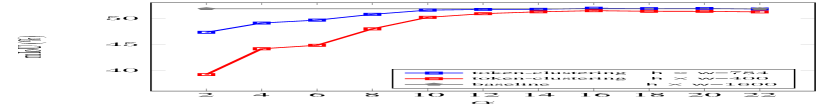
(a) mIoU

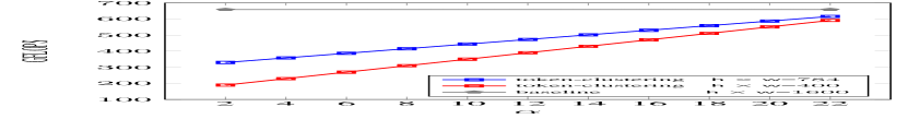
(b) GFLOPs

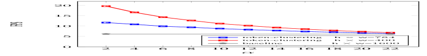
(c) FPS

Figure 4: Influence of the inserted position $\alpha$ of token clustering layer.

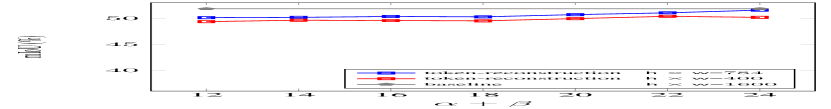
(d) mIoU

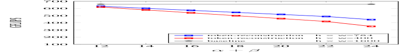
(e) GFLOPs

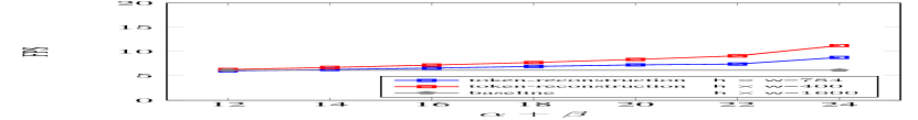
(f) FPS

Figure 5: Influence of the inserted position $\alpha+\beta$ of token reconstruction layer.

4.3 Ablation Study Experiments

We conduct the following ablation experiments on ADE$20$K semantic segmentation benchmark with the official checkpoints of Segmenter+ViT-L/$16$ [63] by default if not specified.

Hyper-parameters of token clustering/reconstruction layer. We first study the influence of the hyper-parameters associated with the token clustering layer, i.e., the number of neighboring pixels $\lambda$ used in Equation 3, the number of EM iterations $\kappa$, and the choice of the temperature $\tau$ in Table 6. According to the results, we can see that our method is relatively less sensitive to the choice of both $\lambda$ and $\kappa$ compared to $\tau$. In summary, we choose $\lambda$ as $5\times 5$, $\kappa$ as $5$, and $\tau$ as $50$ considering both performance and efficiency. Next, we also study the influence of the hyper-parameters within the token clustering layer, i.e., the number of nearest neighbors k within k-NN. We do not observe obvious differences and thus set k as $20$. More details are provided in the supplementary material.

Influence of cluster size choices. We study the influence of different cluster size $\mathsf{h}\times\mathsf{w}$ choices based on input feature map of size $\frac{\mathsf{H}}{\mathsf{P}}\times\frac{\mathsf{W}}{\mathsf{P}}=40\times 40$ ($\mathsf{N}=1,600$) in Table 6. According to the results, we can see that choosing too small cluster sizes significantly harms the dense prediction performance, and setting $\mathsf{h}\times\mathsf{w}$ as $28\times 28$ achieves the better trade-off between performance drop and model complexity. Therefore, we choose $28\times 28$ on Segmenter+ViT-L/$16$ by default. We also empirically find that selecting the cluster size $\mathsf{h}\times\mathsf{w}$ around $\mathsf{N}/4\sim\mathsf{N}/2$ performs better on most of the other experiments. We conduct the following ablation experiments under two typical settings, including $20\times 20$ ($\sim\mathsf{N}/4$) and $28\times 28$ ($\sim\mathsf{N}/2$).

Comparison with adaptive average pooling and bi-linear upsample. We report the comparison results between our proposed token clustering/reconstruction scheme and adaptive average pooling/bi-linear upsample scheme in Table 6 and Table 6 under two cluster size settings respectively. We choose to compare with adaptive average pooling and bi-linear upsample instead of strided convolution or deconvolution as the previous ones are non-parametric and the later ones require re-training or fine-tuning, which are not the focus of this work. Specifically, we keep the inserted position choices the same and only replace the token cluster or token reconstruction layer with adaptive average pooling or bi-linear upsampling under the same cluster size choices. According to the results, we can see that our proposed token clustering and token reconstruction consistently outperform adaptive average pooling and bi-linear upsampling under different cluster size choices.

Influence of inserted position of token clustering/reconstruction layer. We investigate the influence of the inserted position of both token clustering layer and token reconstruction layer and summarize the detailed results in Figure 5 and Figure 5 under two different cluster size choices. According to the results shown in Figure 5, our method achieves better performance when choosing $\alpha$ larger than $10$, therefore, we choose $\alpha=10$ as it achieves a better trade-off between model complexity and segmentation accuracy. Then we study the influence of the inserted positions of the token reconstruction layer by fixing $\alpha=10$. According to Figure 5, we can see that our method achieves the best performance when setting $\alpha+\beta=24$, in other words, we insert the token reconstruction layer after the last transformer layer of ViT-L/$16$. We choose $\alpha=10$, $\alpha+\beta=24$, and $\gamma=0$ for all ablation experiments on ADE$20$K by default if not specified.

Combination with lighter vision transformer architecture. We report the results of applying our method to lighter vision transformer backbones such as ViT-B/$16$, in Table 6. Our approach consistently improves the efficiency of Segmenter+ViT-B/$16$ at the cost of a slight performance drop without fine-tuning. Specifically speaking, our approach saves more than $26\%\downarrow$ GFLOPs of a trained “Segmenter+ViT-B/$16$” with only a slight performance drop from $48.48\%$ to $48.40\%$, which verifies our method also generalizes to lighter vision transformer architectures.

Comparison with uniform downsampling. We compare our method with the simple uniform downsampling scheme, which directly downsamples the input image into a lower resolution. Figure 9 summarizes the detailed comparison results. For example, on ADE$20$K, we downsample the input resolution from $640\times 640$ to smaller resolutions (e.g., $592\times 592$, $576\times 576$, $560\times 560$, and $544\times 544$) and report their performance and GFLOPs in Figure 9. We also plot the results with our method and we can see that our method consistently outperforms uniform sampling on both ADE$20$K and PASCAL-Context under multiple different GFLOPs budgets.

4.4 Object Detection

We use the recent SOTA object detection framework SwinV$2$-L + HTC++ [46] as our baseline. We summarize the results of combining our method with SwinV$2$-L + HTC++ on COCO object detection and instance segmentation tasks in Figure 9.

Implementation details. The original SwinV$2$-L consists of {$2$,$2$,$18$,$2$} shifted window transformer blocks across the four stages. We only apply our method to the $3$-rd stage with $18$ blocks considering it dominates the computation overhead, which we also follow in the “Mask$2$Former + Swin-L” experiments. We insert the window token clustering/reconstruction layer after the $8$-th/$18$-th block within the $3$-rd stage, which are based on the official checkpoints  of SwinV$2$-L + HTC++. In other words, we set $\alpha=12$ and $\alpha+\beta=22$ for SwinV$2$-L. The default window size is $\mathsf{K}\times\mathsf{K}$=$32\times 32$ and we set the clustered window size as $\mathsf{k}\times\mathsf{k}$=$23\times 23$. We choose the values of other hyperparameters following the ablation experiments. According to the results summarized in Figure 9, compared to SwinV$2$-L + HTC++, our method improves the FPS by $21\%\uparrow$ and saves the GFLOPs by nearly $20\%\downarrow$ while maintaining around $98\%$ of object detection & instance segmentation performance.

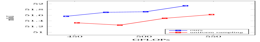
(a) ADE$20$K

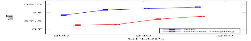
(b) PASCAL-Context

Figure 6: Comparison to uniform downsampling on ADE$20$K and PASCAL-Context with Segmenter+ViT-L/$16$.

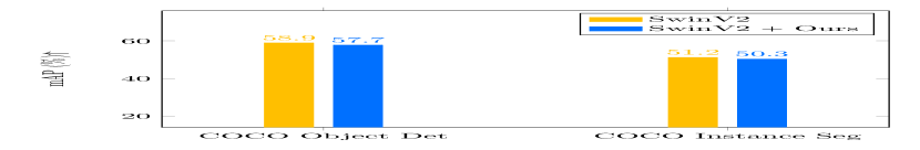
(c) mAP

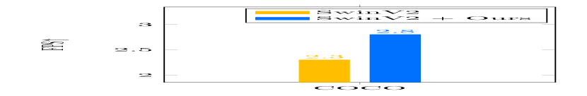
(d) FPS

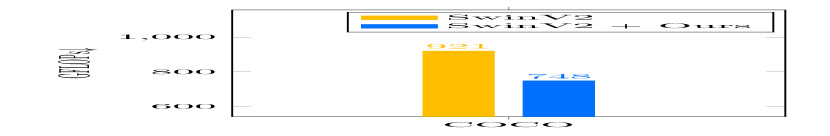
(e) GFLOPs

Figure 7: Illustrating the improvements of our approach on object detection task with SwinV$2$-L + HTC++. $\uparrow$ and $\downarrow$ represent higher is better and lower is better respectively.

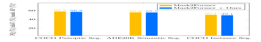
(a) mAP

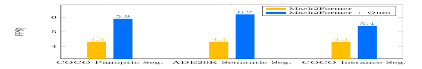
(b) FPS

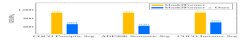
(c) GFLOPs

Figure 8: Illustrating the improvements of our approach on panoptic segmentation, semantic segmentation, and instance segmentation tasks with Mask$2$Former+Swin-L.

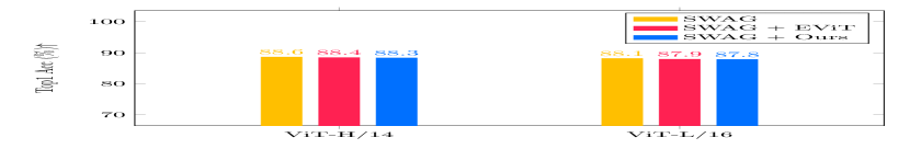
(a) Top-$1$ Accuracy

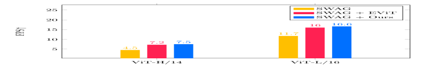
(b) FPS

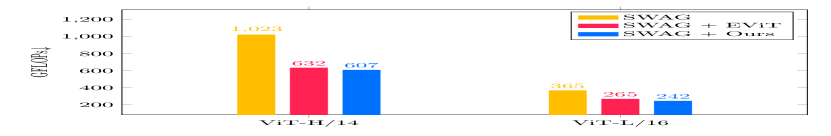
(c) GFLOPs

Figure 9: Illustrating the improvements of our approach and the comparisons with EViT [44] on ImageNet classification tasks with SWAG+ViT-H/$14$ and SWAG+ViT-L/$16$.

4.5 Semantic/Instance/Panoptic Segmentation

We first apply our method to a plain ViT-based segmentation framework Segmenter [63] and illustrate the semantic segmentation results across three benchmarks including ADE$20$K, PASCAL-Context, and Cityscapes on the first row of Figure 1. Then, we apply our method to a very recent framework Mask$2$Former [11] that is based on Swin Transformer and summarize the semantic segmentation, instance segmentation, and panoptic segmentation results on COCO in Figure 9.

Implementation details. The original ViT-L first splits an image into a sequence of image patches of size $16\times 16$ and applies a patch embedding layer to increase the channel dimensions to $1024$, then applies $24$ consecutive transformer encoder layers for representation learning. To apply our method to the ViT-L backbone of Segmenter, we use the official checkpoints  of “Segmenter + ViT-L/$16$” and insert the token clustering layers and token reconstruction layer into the ViT-L/$16$ backbone without fine-tuning.

For the Mask$2$Former built on Swin-L with window size as $12\times 12$, we use the official checkpoints  of “Mask$2$Former + Swin-L” and insert the window token clustering layer and the window token reconstruction layer into the empirically chosen positions, which first cluster $12\times 12$ tokens into $8\times 8$ tokens and then reconstruct $12\times 12$ tokens within each window. Figure 9 summarizes the detailed comparison results. Accordingly, we can see that our method significantly improves the FPS by more than $35\%\uparrow$ with a slight performance drop on COCO panoptic segmentation task.

4.6 Monocular Depth Estimation

To verify the generalization of our approach, we apply our method to depth estimation tasks that measure the distance of each pixel relative to the camera. We choose the DPT (Dense Prediction Transformer) [54] that builds on the hybrid vision transformer, i.e., R$50$+ViT-B/$16$, following [18].

Implementation details. The original R$50$+ViT-B/$16$  consists of a ResNet$50$ followed by a ViT-B/$16$, where the ViT-B/$16$ consists of $12$ transformer encoder layers that process $16\times$ downsampled representations. We insert the token clustering layer & token reconstruction layer into ViT-B/$16$ and summarize the results on both KITTI and NYUv$2$ on the second row of Figure 1. We also report their detailed depth estimation results in Table 7, where we can see that our method accelerates DPT by nearly $30\%$/$37\%\uparrow$ on KITTI/NYUv$2$, respectively.

4.7 ImageNet-$1$K Classification

Finally, we apply our method to the ImageNet-$1$K classification task and compare our method with a very recent SOTA method EViT [44]. The key idea of EViT is to identify and only keep the top-$k$ tokens according to their attention scores relative to the [class] token. We empirically find that applying EViT for dense prediction tasks directly suffers from significant performance drops. More details are illustrated in the supplementary material.

Implementation details. We choose the recent SWAG [61] as our baseline, which exploits $3.6$ billion weakly labeled images associated with around $27$K categories (or hashtags) to pre-train the large-scale vision transformer models, i.e., ViT-L/$16$ and ViT-H/$14$. According to their official implementations , SWAG + ViT-H/$14$ and SWAG + ViT-L/$16$ achieve $88.55\%$ and $88.07\%$ top-$1$ accuracy on ImaegNet-1K respectively. We apply our approach and EViT to both baselines and summarize the comparison results in Figure 9. According to the results, our method achieves comparable results as EViT while being more efficient, which further verifies that our method also generalizes to the image classification tasks without fine-tuning.

Table 7: Depth estimation results based on DPT [54] with ResNet-$50$+ViT-B/$16$.

Dataset	Method	GFLOPs	FPS	$\delta$>$1.25$	$\delta$>$1.25^{2}$	$\delta$>$1.25^{3}$	AbsRel	SqRel	RMSE	RMSElog	SILog	log$10$
KITTI	DPT	$810$	$11.38$	$0.959$	$0.995$	$0.999$	$0.062$	$0.222$	$2.573$	$0.092$	$8.282$	$0.027$
	DPT+Ours	$627$	$14.75$	$0.958$	$0.995$	$0.999$	$0.062$	$0.226$	$2.597$	$0.093$	$8.341$	$0.027$
NYUv$2$	DPT	$560$	$17.58$	$0.904$	$0.988$	$0.998$	$0.110$	$0.054$	$0.357$	$0.129$	$9.522$	$0.045$
	DPT+Ours	$404$	$24.03$	$0.900$	$0.987$	$0.998$	$0.113$	$0.056$	$0.363$	$0.132$	$9.532$	$0.046$

5 Conclusion

In this paper, we present a simple and effective mechanism to improve the efficiency of large-scale vision transformer models for dense prediction tasks. In light of the relatively high costs associated with re-training or fine-tuning large vision transformer models on various dense prediction tasks, our study provides a very lightweight method for expediting the inference process while requiring no additional fine-tuning. We hope our work could inspire further research efforts into exploring how to accelerate large-scale vision transformers for dense prediction tasks without fine-tuning.

Checklist

1. For all authors…

   1. Do the main claims made in the abstract and introduction accurately reflect the paper’s contributions and scope? [Yes]

   2. Have you read the ethics review guidelines and ensured that your paper conforms to them? [Yes]

   3. Did you discuss any potential negative societal impacts of your work? [N/A]

   4. Did you describe the limitations of your work? [N/A]

2. If you are including theoretical results…

   1. Did you state the full set of assumptions of all theoretical results? [N/A]

   2. Did you include complete proofs of all theoretical results? [N/A]

3. If you ran experiments…

   1. Did you include the code, data, and instructions needed to reproduce the main experimental results (either in the supplemental material or as a URL)? [TODO]We will release the code soon.

   2. Did you specify all the training details (e.g., data splits, hyperparameters, how they were chosen)? [Yes]

   3. Did you report error bars (e.g., with respect to the random seed after running experiments multiple times)? [TODO]

   4. Did you include the total amount of compute and the type of resources used (e.g., type of GPUs, internal cluster, or cloud provider)? [Yes]

4. If you are using existing assets (e.g., code, data, models) or curating/releasing new assets…

   1. If your work uses existing assets, did you cite the creators? [Yes] We use the official checkpoints provided by:

      • {https://github.com/rstrudel/segmenter#model-zoo}, MIT License

      • https://github.com/facebookresearch/Mask2Former/blob/main/MODEL_ZOO.md, CC-BY-NC $4.0$

      • https://github.com/microsoft/Swin-Transformer, MIT License

      • https://github.com/facebookresearch/SWAG, CC-BY-NC $4.0$

      • https://github.com/isl-org/DPT, MIT License.

   2. Did you mention the license of the assets? [Yes] We mark the license of these assets as above.

   3. Did you include any new assets either in the supplemental material or as a URL? [Yes] We add the URL of these assets in the footnote.

   4. Did you discuss whether and how consent was obtained from people whose data you’re using/curating? [N/A]

   5. Did you discuss whether the data you are using/curating contains personally identifiable information or offensive content? [N/A]

5. If you used crowdsourcing or conducted research with human subjects…

   1. Did you include the full text of instructions given to participants and screenshots, if applicable? [N/A]

   2. Did you describe any potential participant risks, with links to Institutional Review Board (IRB) approvals, if applicable? [N/A]

   3. Did you include the estimated hourly wage paid to participants and the total amount spent on participant compensation? [N/A]

Appendix

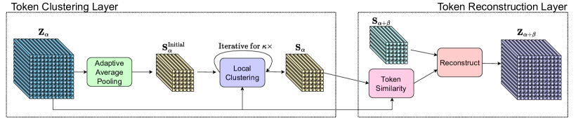
Figure 10: Illustrating more details of our approach. The token clustering layer consists of an adaptive average pooling block (for initializing the cluster centers) and an iterative local clustering block (for performing the k-means clustering). The token reconstruction layer consists of a token similarity estimation block (for estimating the reconstruction relation matrix) and a reconstruction block (for reconstructing the high-resolution representations). $\mathbf{Z}_{\alpha}$ represents the original high-resolution representations after $\alpha$-th transformer layer. $\mathbf{S}_{\alpha}$ represents the clustered low-resolution representations by token clustering layer. $\mathbf{S}_{\alpha+\beta}$ represents the refined clustered low-resolution representations after additional $\beta$ transformer layers. $\mathbf{Z}_{\alpha+\beta}$ represents the reconstructed high-resolution representations from $\mathbf{S}_{\alpha+\beta}$ by using the token reconstruction layer.

Table 8: Illustrating the hyper-parameter settings used for Segmenter, DPT, and SWAG.

Method	Backbone	Dataset	$\alpha$	$\alpha+\beta$	$\gamma$	$\mathsf{L}$	$\frac{\mathsf{H}}{\mathsf{P}}\times\frac{\mathsf{W}}{\mathsf{P}}$	$\mathsf{h}\times\mathsf{w}$	$\lambda$	$\kappa$	$\tau$	$\mathsf{k}$
Segmenter [63]	ViT-L/$16$	ADE$20$K	$10$	$24$	$0$	$24$	$40\times 40$	$28\times 28$	$5\times 5$	$5$	$50$	$20$
		Cityscapes	$12$				$48\times 48$	$32\times 32$
		PASCAL-Context	$14$				$30\times 30$	$15\times 15$
DPT [54]	R$50$+ViT-B/$16$	KITTI	$2$	$12$	$0$	$12$	$76\times 22$	$28\times 28$	$5\times 5$	$5$	$5$	$20$
		NYUv$2$	$3$				$40\times 30$	$16\times 16$	$7\times 7$	$5$	$10$	$50$
SWAG [61]	ViT-H/$14$	ImageNet-$1$K	$8$	$32$	$0$	$32$	$37\times 37$	$25\times 25$	$7\times 7$	$5$	$1$	$20$
	ViT-L/$16$		$8$	$24$	$0$	$24$	$32\times 32$	$22\times 22$	$9\times 9$	$5$	$1$	$20$

Table 9: Illustrating the hyper-parameter settings used for Mask$2$Former and SwinV$2$-L + HTC++.

Method	Backbone	Dataset	$\alpha$	$\alpha+\beta$	$\gamma$	$\mathsf{L}$	$\mathsf{K}\times\mathsf{K}$	$\mathsf{k}\times\mathsf{k}$	$\lambda$	$\kappa$	$\tau$	$\mathsf{k}$
Mask$2$Former [11]	Swin-L	COCO (panoptic seg.)	$10$	$22$	$2$	$24$	$12\times 12$	$8\times 8$	$7\times 7$	$5$	$20$	$10$
		ADE20K (semantic seg.)	$8$						$5\times 5$	$5$	$100$	$10$
		COCO (instance seg.)	$12$						$11\times 11$	$5$	$100$	$60$
SwinV$2$-L + HTC++ [46]	SwinV$2$-L	COCO (object det.)	$12$	$22$	$2$	$24$	$32\times 32$	$23\times 23$	$5\times 5$	$5$	$33$	$20$

Table 10: Illustrating the hyper-parameter settings used for measuring FPS and GFLOPs.

Method	Backbone	with Head	Dataset	Input resolution
Segmenter [63]	ViT-L/$16$	✓	ADE$20$K	$640\times 640$
			Cityscapes	$768\times 768$
			PASCAL-Context	$480\times 480$
DPT [54]	R$50$+ViT-B/$16$	✓	KITTI	$1216\times 352$
			NYUv$2$	$640\times 480$
SWAG [61]	ViT-H/$14$	✓	ImageNet-1K	$518\times 518$
	ViT-L/$16$			$512\times 512$
Mask$2$Former [11]	Swin-L	✗	COCO (panoptic seg.)	$1152\times 1152$
			ADE20K (semantic seg.)	$1152\times 1152$
			COCO (instance seg.)	$1152\times 1152$
SwinV$2$-L + HTC++ [46]	SwinV$2$-L	✗	COCO (object det.)	$1024\times 1024$

Table 11: Comparison to parametric methods based on Segmenter [63].

Dataset	Method	Parametric	Fine-Tuning	GFLOPs	mIoU
ADE$20$K	Dynamic ViT ($\rho=0.7$)	✓	✓	$455.6$	$45.62$
	Dynamic ViT ($\rho=0.8$)	✓	✓	$513.3$	$47.89$
	Dynamic ViT ($\rho=0.9$)	✓	✓	$583.0$	$50.42$
	Ours ($\mathrm{h}\times\mathrm{w}=16\times 16$)	✗	✗	$315.1$	$48.21$
	Ours ($\mathrm{h}\times\mathrm{w}=20\times 20$)	✗	✗	$347.2$	$50.17$
	Ours ($\mathrm{h}\times\mathrm{w}=24\times 24$)	✗	✗	$388.2$	$51.32$

Table 12: Illustrating the differences between clustered attention [68], ACT [89], SMRF [15], and our approach.

22mmCluster method	query	key-value	FFN	#clustering layers
Clustered Attention [68]	✓	✗	✗	# MHSA layers
ACT [89]	✓	✗	✗	# MHSA layers
SMRF [15]	✓	✓	✗	# MHSA layers
Ours	✓	✓	✓	$1$

Table 13: Comparison results with ACT [89].

22mmCluster method	FPS	GFLOPs	mIoU
Segmenter+ViT-B/$16$	$6.2$	$659.0$	$51.82$
Segmenter+ViT-B/$16$+Ours($\mathrm{h}$$\times$$\mathrm{w}$=$24\times 24$)	$9.1$	$388.2$	$51.32$
Segmenter+ViT-B/$16$+Ours($\mathrm{h}$$\times$$\mathrm{w}$=$28\times 28$)	$8.8$	$438.9$	$51.56$
Segmenter+ViT-B/$16$+ACT(#query-hashes=$16$)	$5.8$	$578.7$	$48.12$
Segmenter+ViT-B/$16$+ACT(#query-hashes=$24$)	$5.3$	$614.7$	$51.38$
Segmenter+ViT-B/$16$+ACT(#query-hashes=$32$)	$5.0$	$638.2$	$51.64$

A. Illustrating More Details of Our Approach

We first illustrate the overall details of our token clustering layer and token reconstruction layer in Figure 10. We then present the example implementation of token clustering layer and token reconstruction layer based on PyTorch in Listing LABEL:lst:token_clustering and Listing LABEL:lst:token_reconstruct, respectively.

B. More Hyper-parameter Details

We summarize the detailed hyper-parameter settings for the dense prediction methods based on plain ViTs and Swin Transformers in Table 13 and Table 13, respectively.

Table 13 summarizes the hyper-parameters, including the inserted positions $\alpha$ & $\alpha$+$\beta$ of token clustering layer & token reconstruction layer, the number of remaining transformer layers after the token reconstruction layer $\gamma$, the total number of transformer layers $\mathsf{L}$, the number of tokens before clustering $\frac{\mathsf{H}}{\mathsf{P}}\times\frac{\mathsf{W}}{\mathsf{P}}$, the number of tokens after clustering $\mathsf{h}\times\mathsf{w}$, the number of neighboring pixels $\lambda$, the number of EM iterations $\kappa$, the temperature value $\tau$, and the number of nearest neighbors $\mathsf{k}$, for Segmenter, DPT, and SWAG.

Table 13 summarizes the hyper-parameters, including the inserted positions $\alpha$ & $\alpha$+$\beta$ of the window token clustering layer & window token reconstruction layer, the number of remaining transformer layers after the token reconstruction layer $\gamma$, the total number of transformer layers $\mathsf{L}$, the number of window tokens before clustering $\mathsf{K}\times\mathsf{K}$, the number of window tokens after clustering $\mathsf{k}\times\mathsf{k}$, the number of neighboring pixels $\lambda$, the number of EM iterations $\kappa$, the temperature value $\tau$, and the number of nearest neighbors $\mathsf{k}$, for Mask$2$Former and SwinV$2$-L + HTC++.

C. More Evaluation Details

We illustrate the evaluation details used for measuring the GFLOPs and FPS of different methods in Table 13. We choose the input resolutions for different methods with different backbones according to their official implementations. To illustrate the effectiveness of our method more accurately, we do not include the complexity and latency brought by the especially heavy detection heads or segmentation heads within Mask$2$Former and SwinV$2$-L + HTC++. For example, the GFLOPs of SwinV$2$-L backbone accounts for only $56.7\%$ of the whole model, therefore, we only report the GFLOPs and FPS improvements of our method over the backbone.

D. Comparison with EViT [44] on Dense Prediction

To demonstrate the advantage of our approach over the representative method that is originally designed for the image classification tasks, i.e., EViT [44], we report the detailed comparison results in Figure 12. The original EViT propose to identify and only keep the top $\rho\%$ tokens according to their attention scores relative to the [class] token. Specifically, we follow the official implementations to insert the token identification module into the $8$-th, $14$-th, and $20$-th layer of ViT-L/$16$ (with $24$ layers in total) to decrease the number of tokens by ($1$-$\rho\%$), respectively. We report the results of EViT by choosing $\rho\%$=$60\%$/$70\%$/$80\%$/$90\%$ in Figure 12. Accordingly, we can see that our method significantly outperforms EViT across various GFLOPs & FPS settings when evaluating without either re-training or fine-tuning.

The EViT can not be used for dense prediction directly, as it only keeps around $21.6\%\sim 72.9\%$ of the tokens at last. To reconstruct the missed token representations over the abandoned positions, we apply two different strategies, including (i) reusing the representations before the corresponding token identification module, and (ii) using our token reconstruction layer to reconstruct the missed token representations according to Figure 11(a). We empirically find the first strategy achieves much worse results, thus choosing the second strategy by default.

E. Adapting DynamicViT [55] for Dense Prediction

To adapt DynamicViT for dense prediction tasks, we propose to add multiple token reconstruction layers to reconstruct high-resolution representations from the selected low-resolution representations iteratively. Figure 12 (b) presents more details of the overall framework. We also report the comparison results in Table 13.

F. Comparison with Clustered Attention [68], ACT [89], and SMRF [15]

We illustrate the key differences between our approach and the existing clustered attention approaches [68, 89, 15] the following two aspects: (i) These clustering attention methods perform clustering within each multi-head self-attention layer (MHSA) independently while our approach only performs clustering once with the token clustering layer and refines the clustered representations with the following transformer layers. Therefore, our approach introduces a much smaller additional overhead caused by the clustering operation. (ii) These clustering attention methods only reduce the computation cost of each MHSA layer equipped with clustering attention as they maintain the high-resolution representations outside the MHSA layers while Our approach can reduce the computation cost of both MHSA layers and feed-forward network (FFN) layers after the token clustering layer. We further summarize their detailed differences and the experimental comparison resultswith ACT [89](without retraining) in Table 13 and Table 13, respectively.

According to the results in Table 13, we can see that (i) ACT also achieves strong performance without retraining, (ii) our approach is a better choice considering the trade-off between performance and FPS & GFLOPs, e.g., our method achieves close performance as ACT ($51.32$ vs. $51.38$) while running $70\%$ faster ($9.1$ vs. $5.3$) and saving more than $35\%$ GFLOPs ($388.2$ vs. $614.7$).

G. Visualization

We first present the visual comparison results of our approach in Figure 13(a), which shows three different configurations over Segmenter+ViT-L/$16$ achieve $32.13\%$/$48.21\%$/$51.32\%$ when setting the cluster size $\rm{h}\times\rm{w}$ as $8\times 8$/$16\times 16$/$24\times 24$, respectively.

Then, we visualize both the original feature maps and the clustering feature maps in Figure 13(b). Accordingly, we can see that the clustering feature maps, based on our token clustering layer, well maintain the overall structure information carried in the original high-resolution feature maps.

Last, to verify the redundancy in the tokens of vision transformer, we visualize the attention maps of neighboring tokens in Figure 14.

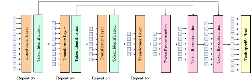
(a) Adapting EViT for Dense Prediction

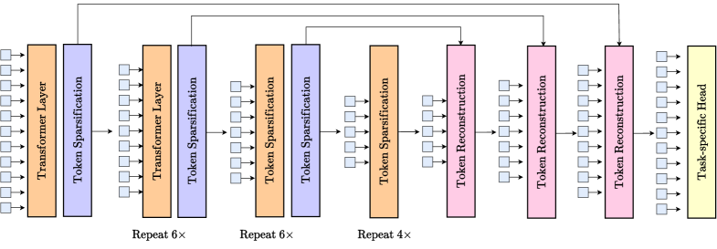
(b) Adapting DynamicViT for Dense Prediction

Figure 11: Illustrating how to adapt the EViT [44] and DynamicViT [55] for dense prediction based on ViT-L/$16$ with $24$ transformer layers. Following the proposed token reconstruction scheme, we estimate the semantic relations based on the representations before each token identification layer [44] or token sparsification layer [55].

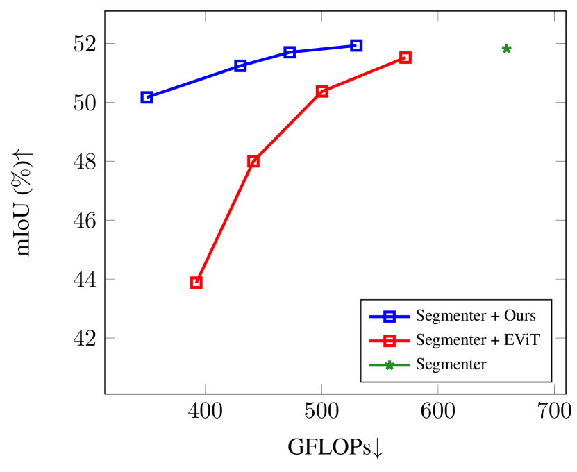
(c) mIoU vs. GFLOPs on ADE$20$K

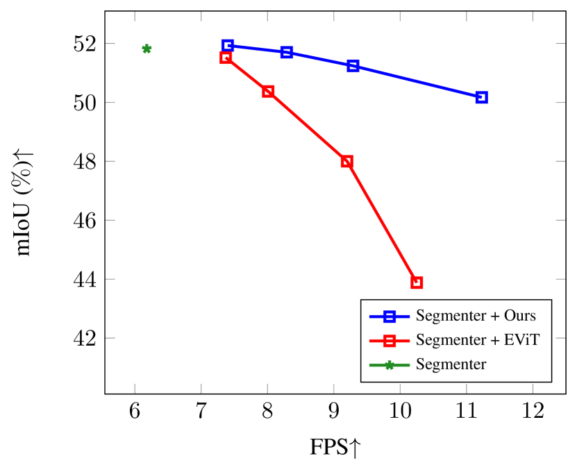
(d) mIoU vs. FPS on ADE$20$K

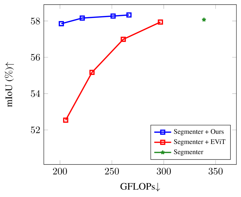
(e) mIoU vs. GFLOPs on PASCAL-Context

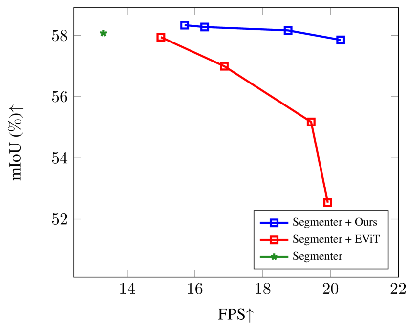
(f) mIoU vs. FPS on PASCAL-Context

Figure 12: Comparison with EViT [44] on ADE$20$K and PASCAL-Context semantic segmentation task based on Segmenter with ViT-L/$16$. $\uparrow$ and $\downarrow$ represent higher is better and lower is better respectively.

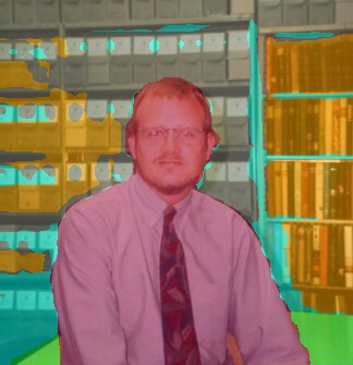
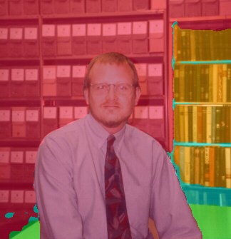
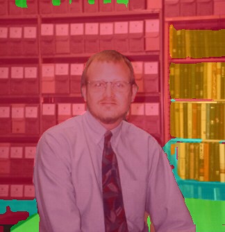
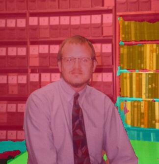
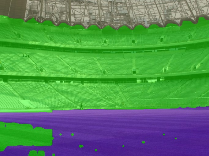
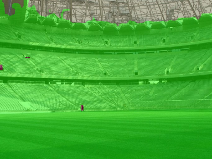
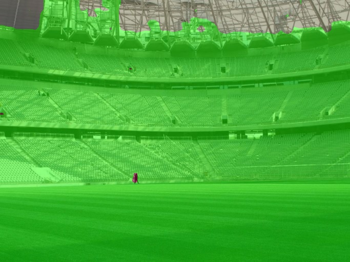
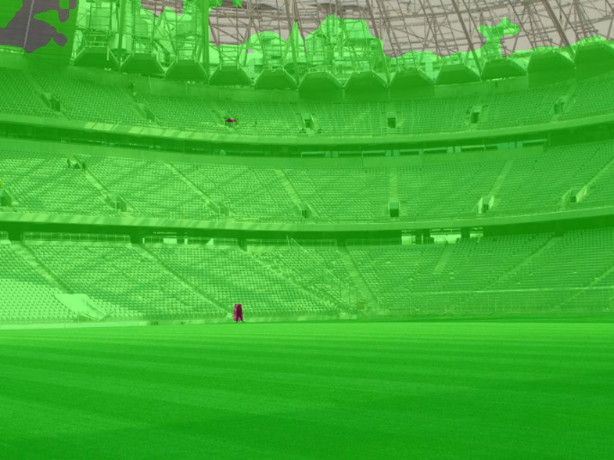
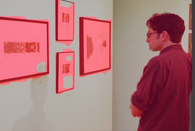
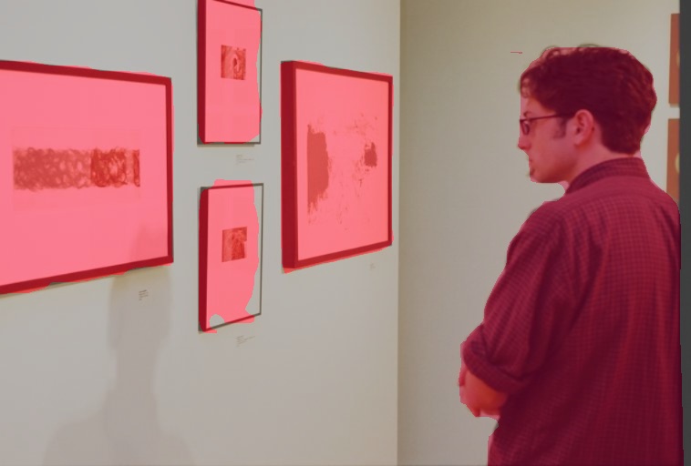
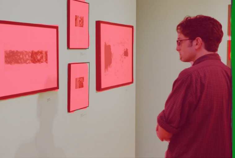
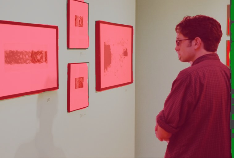
(a) ADE$20$K example segmentation results of our approach with $\rm{h}\times\rm{w}$ as $8\times 8$, $16\times 16$, $24\times 24$ on the left three columns, respectively. The right-most column shows the results of the original Segmenter+ViT-L/$16$. We can see that our approach achieves consistently better segmentation results with increasing clustered output resolutions from left to right.

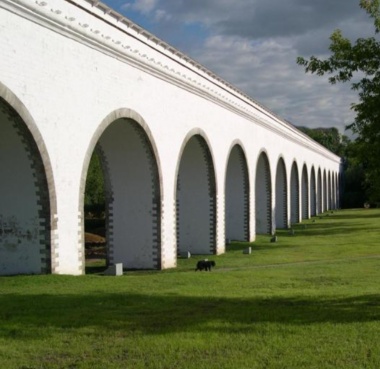
(b) ADE$20$K example visualization of the original feature maps ($2$-ed row) and the clustering feature maps ($3$-rd row). We can see that the clustering feature maps still maintain the structure information presented in the original high-resolution feature maps, thus showing the potential benefits of our token clustering scheme.

Figure 13: Visualizations of segmentation results in (a) and feature maps in (b). We choose Segmenter+ViT-L/$16$ on ADE$20$K to generate the above segmentation results and the feature map visualizations.

Figure 14: Visualizations of the attention maps of neighboring sampled positions. We mark the sampled positions with red point markers. We can see that the neighboring positions share highly similar attention maps, which matches the redundancy observation in the Adaptive Clustering Transformer (ACT) [89].

⬇

1def token_clustering_layer(features, cluster_features_shape, num_iters, tau):

2 # args:

3 # features: shape [B, C, H, W]

4 # cluster_features_shape: [h, w]

5 # num_iters: num of iterations of updating cluster features

6 # teu: the temperture of distance matrix

7 # output:

8 # cluster_features: shape [B, hw, C]

9

10 B, C, H, W = features.shape

11

12 # initialize the cluster features

13 cluster_features = interpolate(features, cluster_features_shape)

14

15 # construct mask to constrain the interactions within local range

16 mask = calculate_mask(features.shape, cluster_features_shape)

17 mask = (~mask) * 1e16

18

19 features = features.reshape(B, C, -1).permute(0, 2, 1) # (B, HW, C)

20 cluster_features = cluster_features.reshape(B, C, -1).permute(0, 2, 1) # (B, hw, C)

21

22 for _ in range(num_iters):

23 # calculate L2 distance of features and cluster features, the shape distance_matrix is (B, hw, HW)

24 distance_matrix = L2_distance(features, cluster_features)

25 # mask remote distance through softmax

26 distance_matrix += mask

27 weights = (-distance_matrix / teu).softmax(dim=1)

28 # let the sum of weight of each cluster feature be 1

29 weights = weights / weights.sum(dim=2, keepdim=True).clamp_(min=1e-16)

30 cluster_features = matrix_product(weights, features)

31

32 return cluster_features

Listing 1: PyTorch example of token clustering layer.

⬇

1def token_reconstruction_layer(cluster_features, features_before_clustering, features_after_clustering, k, teu):

2 # args:

3 # cluster_features: shape [B, hw, C]

4 # features_before_clustering: features of alpha-th layer before clustering, shape [B, hw, C]

5 # features_after_clustering: features of alpha-th layer before clustering, shape [B, HW, C]

6 # k: topk parameter

7 # teu: the temperture of weight matrix

8 # output:

9 # features: reconstruction features, shape [B, HW, C]

10

11 # calculate L2 distance between features and cluster_features

12 distance = L2_distance(features_before_clustering, features_after_clustering)

13 weight = exp(-teu * distance)

14 # only remain the k weight of the most simliar features, calculating mask

15 topk, indices = topk(weight, k=k, dim=2)

16 mink = min(topk, dim=-1).values

17 mink = mink.unsqueeze(-1).repeat(1, 1, weight.shape[-1])

18 mask = greater_or_equal(weight, mink)

19 weight = weight * mask

20

21 weight = weight / weight.sum(dim=2, keepdim=True).clamp_(min=1e-16)

22 features = matrix_product(weight, cluster_features)

23

24 return features

Listing 2: PyTorch example of token reconstruction layer.

References

- [1] Hangbo Bao, Li Dong, and Furu Wei. Beit: Bert pre-training of image transformers. arXiv preprint arXiv:2106.08254, 2021.
- [2] Davis Blalock, Jose Javier Gonzalez Ortiz, Jonathan Frankle, and John Guttag. What is the state of neural network pruning? Proceedings of machine learning and systems, 2:129–146, 2020.
- [3] Walid Bousselham, Guillaume Thibault, Lucas Pagano, Archana Machireddy, Joe Gray, Young Hwan Chang, and Xubo Song. Efficient self-ensemble framework for semantic segmentation. arXiv preprint arXiv:2111.13280, 2021.
- [4] Nicolas Carion, Francisco Massa, Gabriel Synnaeve, Nicolas Usunier, Alexander Kirillov, and Sergey Zagoruyko. End-to-end object detection with Transformers. In ECCV, 2020.
- [5] Arnav Chavan, Zhiqiang Shen, Zhuang Liu, Zechun Liu, Kwang-Ting Cheng, and Eric Xing. Vision transformer slimming: Multi-dimension searching in continuous optimization space. arXiv preprint arXiv:2201.00814, 2022.
- [6] Minghao Chen, Houwen Peng, Jianlong Fu, and Haibin Ling. Autoformer: Searching transformers for visual recognition. In ICCV, pages 12270–12280, 2021.
- [7] Tianlong Chen, Yu Cheng, Zhe Gan, Lu Yuan, Lei Zhang, and Zhangyang Wang. Chasing sparsity in vision transformers: An end-to-end exploration. NeurIPS, 34, 2021.
- [8] Wuyang Chen, Xianzhi Du, Fan Yang, Lucas Beyer, Xiaohua Zhai, Tsung-Yi Lin, Huizhong Chen, Jing Li, Xiaodan Song, Zhangyang Wang, et al. A simple single-scale vision transformer for object localization and instance segmentation. arXiv preprint arXiv:2112.09747, 2021.
- [9] Wuyang Chen, Wei Huang, Xianzhi Du, Xiaodan Song, Zhangyang Wang, and Denny Zhou. Auto-scaling vision transformers without training. In International Conference on Learning Representations, 2021.
- [10] Yinpeng Chen, Xiyang Dai, Dongdong Chen, Mengchen Liu, Xiaoyi Dong, Lu Yuan, and Zicheng Liu. Mobile-former: Bridging mobilenet and transformer. arXiv preprint arXiv:2108.05895, 2021.
- [11] Bowen Cheng, Ishan Misra, Alexander G. Schwing, Alexander Kirillov, and Rohit Girdhar. Masked-attention mask transformer for universal image segmentation. 2022.
- [12] Krzysztof Choromanski, Valerii Likhosherstov, David Dohan, Xingyou Song, Andreea Gane, Tamas Sarlos, Peter Hawkins, Jared Davis, Afroz Mohiuddin, Lukasz Kaiser, et al. Rethinking attention with performers. arXiv preprint arXiv:2009.14794, 2020.
- [13] Marius Cordts, Mohamed Omran, Sebastian Ramos, Timo Rehfeld, Markus Enzweiler, Rodrigo Benenson, Uwe Franke, Stefan Roth, and Bernt Schiele. The Cityscapes dataset for semantic urban scene understanding. In CVPR, 2016.
- [14] Zihang Dai, Hanxiao Liu, Quoc V Le, and Mingxing Tan. Coatnet: Marrying convolution and attention for all data sizes. NeurIPS, 34:3965–3977, 2021.
- [15] Giannis Daras, Nikita Kitaev, Augustus Odena, and Alexandros G Dimakis. Smyrf-efficient attention using asymmetric clustering. NeurIPS, 33:6476–6489, 2020.
- [16] Henghui Ding, Chang Liu, Suchen Wang, and Xudong Jiang. Vision-language transformer and query generation for referring segmentation. In ICCV, pages 16321–16330, 2021.
- [17] Mingyu Ding, Bin Xiao, Noel Codella, Ping Luo, Jingdong Wang, and Lu Yuan. Davit: Dual attention vision transformer. arXiv preprint arXiv:2204.03645, 2022.
- [18] Alexey Dosovitskiy, Lucas Beyer, Alexander Kolesnikov, Dirk Weissenborn, Xiaohua Zhai, Thomas Unterthiner, Mostafa Dehghani, Matthias Minderer, Georg Heigold, Sylvain Gelly, et al. An image is worth 16x16 words: Transformers for image recognition at scale. arXiv preprint arXiv:2010.11929, 2020.
- [19] Stéphane d’Ascoli, Hugo Touvron, Matthew L Leavitt, Ari S Morcos, Giulio Biroli, and Levent Sagun. Convit: Improving vision transformers with soft convolutional inductive biases. In ICML, pages 2286–2296. PMLR, 2021.
- [20] Alaaeldin El-Nouby, Hugo Touvron, Mathilde Caron, Piotr Bojanowski, Matthijs Douze, Armand Joulin, Ivan Laptev, Natalia Neverova, Gabriel Synnaeve, Jakob Verbeek, et al. Xcit: Cross-covariance image transformers. arXiv preprint arXiv:2106.09681, 2021.
- [21] Haoqi Fan, Bo Xiong, Karttikeya Mangalam, Yanghao Li, Zhicheng Yan, Jitendra Malik, and Christoph Feichtenhofer. Multiscale vision transformers. In ICCV, pages 6824–6835, 2021.
- [22] Andreas Geiger, Philip Lenz, and Raquel Urtasun. Are we ready for autonomous driving? the kitti vision benchmark suite. In 2012 IEEE conference on computer vision and pattern recognition, pages 3354–3361. IEEE, 2012.
- [23] Jiaqi Gu, Hyoukjun Kwon, Dilin Wang, Wei Ye, Meng Li, Yu-Hsin Chen, Liangzhen Lai, Vikas Chandra, and David Z Pan. Hrvit: Multi-scale high-resolution vision transformer. arXiv preprint arXiv:2111.01236, 2021.
- [24] John Guibas, Morteza Mardani, Zongyi Li, Andrew Tao, Anima Anandkumar, and Bryan Catanzaro. Efficient token mixing for transformers via adaptive fourier neural operators. In International Conference on Learning Representations, 2021.
- [25] Kai Han, Yunhe Wang, Qiulin Zhang, Wei Zhang, Chunjing Xu, and Tong Zhang. Model rubik’s cube: Twisting resolution, depth and width for tinynets. NeurIPS, 33:19353–19364, 2020.
- [26] Haodi He, Yuhui Yuan, Xiangyu Yue, and Han Hu. Mlseg: Image and video segmentation as multi-label classification and selected-label pixel classification. arXiv preprint arXiv:2203.04187, 2022.
- [27] Kaiming He, Xinlei Chen, Saining Xie, Yanghao Li, Piotr Dollár, and Ross Girshick. Masked autoencoders are scalable vision learners. arXiv preprint arXiv:2111.06377, 2021.
- [28] Kaiming He, Xiangyu Zhang, Shaoqing Ren, and Jian Sun. Deep Residual Learning for Image Recognition. In CVPR, 2016.
- [29] Byeongho Heo, Sangdoo Yun, Dongyoon Han, Sanghyuk Chun, Junsuk Choe, and Seong Joon Oh. Rethinking spatial dimensions of vision transformers. In ICCV, pages 11936–11945, 2021.
- [30] Torsten Hoefler, Dan Alistarh, Tal Ben-Nun, Nikoli Dryden, and Alexandra Peste. Sparsity in deep learning: Pruning and growth for efficient inference and training in neural networks. JMLR, 22(241):1–124, 2021.
- [31] Zejiang Hou and Sun-Yuan Kung. Multi-dimensional model compression of vision transformer. arXiv preprint arXiv:2201.00043, 2021.
- [32] Jitesh Jain, Anukriti Singh, Nikita Orlov, Zilong Huang, Jiachen Li, Steven Walton, and Humphrey Shi. Semask: Semantically masked transformers for semantic segmentation. arXiv preprint arXiv:2112.12782, 2021.
- [33] Varun Jampani, Deqing Sun, Ming-Yu Liu, Ming-Hsuan Yang, and Jan Kautz. Superpixel sampling networks. In ECCV, pages 352–368, 2018.
- [34] Chao Jia, Yinfei Yang, Ye Xia, Yi-Ting Chen, Zarana Parekh, Hieu Pham, Quoc Le, Yun-Hsuan Sung, Zhen Li, and Tom Duerig. Scaling up visual and vision-language representation learning with noisy text supervision. In ICML, pages 4904–4916. PMLR, 2021.
- [35] Kumara Kahatapitiya and Michael S Ryoo. Swat: Spatial structure within and among tokens. arXiv preprint arXiv:2111.13677, 2021.
- [36] Nikita Kitaev, Łukasz Kaiser, and Anselm Levskaya. Reformer: The efficient transformer. arXiv preprint arXiv:2001.04451, 2020.
- [37] Zhenglun Kong, Peiyan Dong, Xiaolong Ma, Xin Meng, Wei Niu, Mengshu Sun, Bin Ren, Minghai Qin, Hao Tang, and Yanzhi Wang. Spvit: Enabling faster vision transformers via soft token pruning. arXiv preprint arXiv:2112.13890, 2021.
- [38] Liunian Harold Li*, Pengchuan Zhang*, Haotian Zhang*, Jianwei Yang, Chunyuan Li, Yiwu Zhong, Lijuan Wang, Lu Yuan, Lei Zhang, Jenq-Neng Hwang, Kai-Wei Chang, and Jianfeng Gao. Grounded language-image pre-training. In CVPR, 2022.
- [39] Yanghao Li, Hanzi Mao, Ross Girshick, and Kaiming He. Exploring plain vision transformer backbones for object detection. arXiv preprint arXiv:2203.16527, 2022.
- [40] Yanghao Li, Chao-Yuan Wu, Haoqi Fan, Karttikeya Mangalam, Bo Xiong, Jitendra Malik, and Christoph Feichtenhofer. Improved multiscale vision transformers for classification and detection. arXiv preprint arXiv:2112.01526, 2021.
- [41] Yanghao Li, Saining Xie, Xinlei Chen, Piotr Dollar, Kaiming He, and Ross Girshick. Benchmarking detection transfer learning with vision transformers. arXiv preprint arXiv:2111.11429, 2021.
- [42] Zhenyu Li, Zehui Chen, Xianming Liu, and Junjun Jiang. Depthformer: Depthformer: Exploiting long-range correlation and local information for accurate monocular depth estimation. arXiv preprint arXiv:2203.14211, 2022.
- [43] Jingyun Liang, Jiezhang Cao, Guolei Sun, Kai Zhang, Luc Van Gool, and Radu Timofte. Swinir: Image restoration using swin transformer. arXiv preprint arXiv:2108.10257, 2021.
- [44] Youwei Liang, GE Chongjian, Zhan Tong, Yibing Song, Jue Wang, and Pengtao Xie. Evit: Expediting vision transformers via token reorganizations. In International Conference on Learning Representations, 2022.
- [45] Tsung-Yi Lin, Michael Maire, Serge Belongie, James Hays, Pietro Perona, Deva Ramanan, Piotr Dollár, and C Lawrence Zitnick. Microsoft coco: Common objects in context. In ECCV, pages 740–755. Springer, 2014.
- [46] Ze Liu, Han Hu, Yutong Lin, Zhuliang Yao, Zhenda Xie, Yixuan Wei, Jia Ning, Yue Cao, Zheng Zhang, Li Dong, et al. Swin transformer v2: Scaling up capacity and resolution. arXiv preprint arXiv:2111.09883, 2021.
- [47] Ze Liu, Yutong Lin, Yue Cao, Han Hu, Yixuan Wei, Zheng Zhang, Stephen Lin, and Baining Guo. Swin transformer: Hierarchical vision transformer using shifted windows. In ICCV, pages 10012–10022, 2021.
- [48] Zhuang Liu, Jianguo Li, Zhiqiang Shen, Gao Huang, Shoumeng Yan, and Changshui Zhang. Learning efficient convolutional networks through network slimming. In Proceedings of the IEEE international conference on computer vision, pages 2736–2744, 2017.
- [49] Zhuang Liu, Mingjie Sun, Tinghui Zhou, Gao Huang, and Trevor Darrell. Rethinking the value of network pruning. arXiv preprint arXiv:1810.05270, 2018.
- [50] Dmitrii Marin, Jen-Hao Rick Chang, Anurag Ranjan, Anish Prabhu, Mohammad Rastegari, and Oncel Tuzel. Token pooling in vision transformers. arXiv preprint arXiv:2110.03860, 2021.
- [51] Sachin Mehta and Mohammad Rastegari. Mobilevit: light-weight, general-purpose, and mobile-friendly vision transformer. arXiv preprint arXiv:2110.02178, 2021.
- [52] Roozbeh Mottaghi, Xianjie Chen, Xiaobai Liu, Nam-Gyu Cho, Seong-Whan Lee, Sanja Fidler, Raquel Urtasun, and Alan L. Yuille. The role of context for object detection and semantic segmentation in the wild. In CVPR, 2014.
- [53] Alec Radford, Jong Wook Kim, Chris Hallacy, Aditya Ramesh, Gabriel Goh, Sandhini Agarwal, Girish Sastry, Amanda Askell, Pamela Mishkin, Jack Clark, et al. Learning transferable visual models from natural language supervision. In ICML, pages 8748–8763. PMLR, 2021.
- [54] René Ranftl, Alexey Bochkovskiy, and Vladlen Koltun. Vision transformers for dense prediction. In ICCV, pages 12179–12188, 2021.
- [55] Yongming Rao, Wenliang Zhao, Benlin Liu, Jiwen Lu, Jie Zhou, and Cho-Jui Hsieh. Dynamicvit: Efficient vision transformers with dynamic token sparsification. arXiv preprint arXiv:2106.02034, 2021.
- [56] Cedric Renggli, André Susano Pinto, Neil Houlsby, Basil Mustafa, Joan Puigcerver, and Carlos Riquelme. Learning to merge tokens in vision transformers. arXiv preprint arXiv:2202.12015, 2022.
- [57] Aurko Roy, Mohammad Saffar, Ashish Vaswani, and David Grangier. Efficient content-based sparse attention with routing transformers. ACL, 9:53–68, 2021.
- [58] Michael Ryoo, AJ Piergiovanni, Anurag Arnab, Mostafa Dehghani, and Anelia Angelova. Tokenlearner: Adaptive space-time tokenization for videos. NeurIPS, 34, 2021.
- [59] Nathan Silberman, Derek Hoiem, Pushmeet Kohli, and Rob Fergus. Indoor segmentation and support inference from rgbd images. In ECCV, pages 746–760. Springer, 2012.
- [60] Karen Simonyan and Andrew Zisserman. Very deep convolutional networks for large-scale image recognition. arXiv preprint arXiv:1409.1556, 2014.
- [61] Mannat Singh, Laura Gustafson, Aaron Adcock, Vinicius de Freitas Reis, Bugra Gedik, Raj Prateek Kosaraju, Dhruv Mahajan, Ross Girshick, Piotr Dollár, and Laurens van der Maaten. Revisiting weakly supervised pre-training of visual perception models, 2022.
- [62] Lin Song, Songyang Zhang, Songtao Liu, Zeming Li, Xuming He, Hongbin Sun, Jian Sun, and Nanning Zheng. Dynamic grained encoder for vision transformers. NeurIPS, 34, 2021.
- [63] Robin Strudel, Ricardo Garcia, Ivan Laptev, and Cordelia Schmid. Segmenter: Transformer for semantic segmentation. arXiv preprint arXiv:2105.05633, 2021.
- [64] Christian Szegedy, Wei Liu, Yangqing Jia, Pierre Sermanet, Scott Reed, Dragomir Anguelov, Dumitru Erhan, Vincent Vanhoucke, and Andrew Rabinovich. Going deeper with convolutions. In CVPR, pages 1–9, 2015.
- [65] Mingxing Tan and Quoc Le. Efficientnet: Rethinking model scaling for convolutional neural networks. In ICML, pages 6105–6114. PMLR, 2019.
- [66] Yi Tay, Mostafa Dehghani, Dara Bahri, and Donald Metzler. Efficient transformers: A survey. arXiv preprint arXiv:2009.06732, 2020.
- [67] Ashish Vaswani, Noam Shazeer, Niki Parmar, Jakob Uszkoreit, Llion Jones, Aidan N Gomez, Łukasz Kaiser, and Illia Polosukhin. Attention is all you need. NeurIPS, 30, 2017.
- [68] Apoorv Vyas, Angelos Katharopoulos, and François Fleuret. Fast transformers with clustered attention. NeurIPS, 33, 2020.
- [69] Tao Wang, Li Yuan, Yunpeng Chen, Jiashi Feng, and Shuicheng Yan. Pnp-detr: towards efficient visual analysis with transformers. In ICCV, pages 4661–4670, 2021.
- [70] Wenhai Wang, Enze Xie, Xiang Li, Deng-Ping Fan, Kaitao Song, Ding Liang, Tong Lu, Ping Luo, and Ling Shao. Pyramid vision transformer: A versatile backbone for dense prediction without convolutions. In ICCV, pages 568–578, 2021.
- [71] Wenxiao Wang, Minghao Chen, Shuai Zhao, Long Chen, Jinming Hu, Haifeng Liu, Deng Cai, Xiaofei He, and Wei Liu. Accelerate cnns from three dimensions: A comprehensive pruning framework. In ICML, pages 10717–10726. PMLR, 2021.
- [72] Wenxiao Wang, Shuai Zhao, Minghao Chen, Jinming Hu, Deng Cai, and Haifeng Liu. Dbp: discrimination based block-level pruning for deep model acceleration. arXiv preprint arXiv:1912.10178, 2019.
- [73] Yulin Wang, Rui Huang, Shiji Song, Zeyi Huang, and Gao Huang. Not all images are worth 16x16 words: Dynamic transformers for efficient image recognition. NeurIPS, 34, 2021.
- [74] Mitchell Wortsman, Gabriel Ilharco, Samir Yitzhak Gadre, Rebecca Roelofs, Raphael Gontijo-Lopes, Ari S Morcos, Hongseok Namkoong, Ali Farhadi, Yair Carmon, Simon Kornblith, et al. Model soups: averaging weights of multiple fine-tuned models improves accuracy without increasing inference time. arXiv preprint arXiv:2203.05482, 2022.
- [75] Enze Xie, Wenhai Wang, Zhiding Yu, Anima Anandkumar, Jose M Alvarez, and Ping Luo. Segformer: Simple and efficient design for semantic segmentation with transformers. NeurIPS, 34, 2021.
- [76] Zhenda Xie, Zheng Zhang, Yue Cao, Yutong Lin, Jianmin Bao, Zhuliang Yao, Qi Dai, and Han Hu. Simmim: A simple framework for masked image modeling. arXiv preprint arXiv:2111.09886, 2021.
- [77] Yufei Xu, Jing Zhang, Qiming Zhang, and Dacheng Tao. Vitpose: Simple vision transformer baselines for human pose estimation. arXiv preprint arXiv:2204.12484, 2022.
- [78] Jianwei Yang, Chunyuan Li, Pengchuan Zhang, Xiyang Dai, Bin Xiao, Lu Yuan, and Jianfeng Gao. Focal self-attention for local-global interactions in vision transformers. arXiv preprint arXiv:2107.00641, 2021.
- [79] Jiahui Yu, Linjie Yang, Ning Xu, Jianchao Yang, and Thomas Huang. Slimmable neural networks. arXiv preprint arXiv:1812.08928, 2018.
- [80] Yuhui Yuan, Xilin Chen, and Jingdong Wang. Object-contextual representations for semantic segmentation. In ECCV, pages 173–190. Springer, 2020.
- [81] Yuhui Yuan, Rao Fu, Lang Huang, Weihong Lin, Chao Zhang, Xilin Chen, and Jingdong Wang. Hrformer: High-resolution transformer for dense prediction. arXiv preprint arXiv:2110.09408, 2021.
- [82] Yuhui Yuan, Lang Huang, Jianyuan Guo, Chao Zhang, Xilin Chen, and Jingdong Wang. Ocnet: Object context network for scene parsing. arXiv preprint arXiv:1809.00916, 2018.
- [83] Yuhui Yuan, Jingyi Xie, Xilin Chen, and Jingdong Wang. Segfix: Model-agnostic boundary refinement for segmentation. In ECCV. Springer, 2020.
- [84] Xiaohua Zhai, Alexander Kolesnikov, Neil Houlsby, and Lucas Beyer. Scaling vision transformers. CVPR, 2022.
- [85] Bowen Zhang, Shuyang Gu, Bo Zhang, Jianmin Bao, Dong Chen, Fang Wen, Yong Wang, and Baining Guo. Styleswin: Transformer-based gan for high-resolution image generation. arXiv preprint arXiv:2112.10762, 2021.
- [86] Hao Zhang, Feng Li, Shilong Liu, Lei Zhang, Hang Su, Jun Zhu, Lionel M Ni, and Heung-Yeung Shum. Dino: Detr with improved denoising anchor boxes for end-to-end object detection. arXiv preprint arXiv:2203.03605, 2022.
- [87] Haokui Zhang, Wenze Hu, and Xiaoyu Wang. Edgeformer: Improving light-weight convnets by learning from vision transformers. arXiv preprint arXiv:2203.03952, 2022.
- [88] Pengchuan Zhang, Xiyang Dai, Jianwei Yang, Bin Xiao, Lu Yuan, Lei Zhang, and Jianfeng Gao. Multi-scale vision longformer: A new vision transformer for high-resolution image encoding. In ICCV, pages 2998–3008, 2021.
- [89] Minghang Zheng, Peng Gao, Renrui Zhang, Kunchang Li, Xiaogang Wang, Hongsheng Li, and Hao Dong. End-to-end object detection with adaptive clustering transformer. arXiv preprint arXiv:2011.09315, 2020.
- [90] Bolei Zhou, Hang Zhao, Xavier Puig, Tete Xiao, Sanja Fidler, Adela Barriuso, and Antonio Torralba. Semantic understanding of scenes through the ADE20K dataset. IJCV, 2019.