Belief propagation generalizes backpropagation

Abstract

The two most important algorithms in artificial intelligence are backpropagation and belief propagation. In spite of their importance, the connection between them is poorly characterized. We show that when an input to backpropagation is converted into an input to belief propagation so that (loopy) belief propagation can be run on it, then the result of belief propagation encodes the result of backpropagation; thus backpropagation is recovered as a special case of belief propagation. In other words, we prove for apparently the first time that belief propagation generalizes backpropagation. Our analysis is a theoretical contribution, which we motivate with the expectation that it might reconcile our understandings of each of these algorithms, and serve as a guide to engineering researchers seeking to improve the behavior of systems that use one or the other.

1 Introduction

In this paper we consider a connection between two algorithms which could be said to have the status of being the two most fundamental algorithms in the various fields of computer science concerned with the numerical modeling of real world systems, these fields being sometimes known as artificial intelligence or machine learning, sometimes called control theory or statistical modeling or approximate inference. The two algorithms that form our subject matter are usually referred to as backpropagation and belief propagation, respectively, although these are modern terms for concepts that go back several hundred years in Western thought [1, 2, 3].

Back-propagation is another name for the chain rule of differential calculus [4], applied iteratively to a network of functions, or in other words to a function of functions of multiple independent variables and other such functions; the input to backpropagation may also be known in the field as a “deep network” or a “neural network” [5].

Belief propagation, by contrast, takes as its input a network of probability distributions, also called a probabilistic network. Belief propagation is equivalent to an iterative application of Bayes’ rule, which is the rule for inferring the posterior distribution $P(X|Y)$ of a random variable $X$ from its prior $P(X)$ and some table of conditional probabilities $P(Y|X)$ describing the possible observations of some related variable $Y$: $P(X|Y)$ = ${1\over Z(Y)}P(X)P(Y|X)$, often stated as $P(X|Y)={P(X)P(Y|X)\over P(Y)}$ [6, 7]. Belief propagation forbids the sharing of variables among multiple tables of conditionals in its input, implying that there must be no loops in the network, but the symmetry between the posteriors $P(X|Y)$ and the possible observations $P(Y|X)$ allows this dynamic programming algorithm to be recast as a sequence of “message updates” which apply equally well to networks with variable sharing and therefore loops, as was observed by Pearl in the 1980s [8]. The generalized, message-based form of belief propagation is called “loopy belief propagation” [9] (it is also called the “sum-product algorithm” [10]), and while this generalization can no longer be said to compute exact posteriors for its variables, its numerical behavior and its usefulness in approximation have been the object of much study, and it enjoys widespread application in certain specialized domains such as error correcting codes [11, 12]. Loopy belief propagation, to restate the above definition, is “exact on trees”, a tree being a network with no loops, in which case loopy belief propagation reduces to belief propagation. Its theoretical properties are otherwise difficult to characterize [13], and much research has been directed towards improving the accuracy of belief propagation by accounting for the presence of loops in the input model [14, 15, 16, 17, 18].

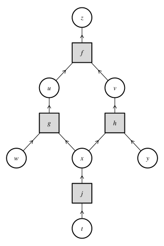
Figure 1: Example network

This paper considers another class of inputs for which loopy belief propagation computes exact quantities, namely probabilistic networks that arise through a straightforward “lifting” of function networks. It is simple to show that the “delta function” posteriors computed by loopy belief propagation on these networks are exact, as they are just a probabilistic representation of the deterministic computation embodied in the original function network. Moreover, we show for the first time that when the output node of the lifted network is attached to a Boltzmann distribution [25, 26] prior, the messages that propagate backwards through the network encode a representation of the exact derivatives of the output variable with respect to each other variable, making loopy belief propagation on the lifted network an extended or lifted form of backpropagation on the original function network. This second result is the main contribution of the paper, establishing that belief propagation is a generalization of backpropagation.

2 Example model

We find it useful to introduce the concepts of this paper through a small example function network. We define a network containing a single loop, and a single shared variable $x$, from the following equations:

$$z=f(u,v)\quad u=g(w,x)\quad v=h(x,y)\quad x=j(t)$$ (1)

The network is illustrated in figure 1.

3 Backpropagation

Running backpropagation on this function network means calculating the derivative of $z$ with respect to the six other variables recursively using the chain rule of differential calculus, starting with the variable $u$

$$\frac{\mathrm{d}z}{\mathrm{d}u}={\partial z\over\partial u}\equiv{\partial f\over\partial u}\equiv f^{(u)}(u,v)$$ (2)

where we have used “$\equiv$” to show the equivalence of alternate notations for partial derivatives. Then for $v$ we have

$$\frac{\mathrm{d}z}{\mathrm{d}v}=f^{(v)}(u,v)$$ (3)

and for $w$

$$\frac{\mathrm{d}z}{\mathrm{d}w}=\frac{\mathrm{d}z}{\mathrm{d}u}{\partial u\over\partial w}\equiv\frac{\mathrm{d}z}{\mathrm{d}u}g^{(w)}(w,x)$$ (4)

and so on. The term “adjoint” is used as a shorthand: since $\mathrm{d}z$ always appears in the numerator in backpropagation, rather than write “the derivative of $z$ with respect to $w$” we call this quantity “the adjoint of $w$ [with respect to $z$]” [27]. Calculating the adjoint of $x$ requires our first addition:

$$\frac{\mathrm{d}z}{\mathrm{d}x}=\frac{\mathrm{d}z}{\mathrm{d}u}{\partial u\over\partial x}+\frac{\mathrm{d}z}{\mathrm{d}v}{\partial v\over\partial x}\equiv\frac{\mathrm{d}z}{\mathrm{d}u}g^{(x)}(w,x)+\frac{\mathrm{d}z}{\mathrm{d}v}h^{(x)}(x,y)$$ (5)

The last adjoint to be calculated is $t$:

$$\frac{\mathrm{d}z}{\mathrm{d}t}=\frac{\mathrm{d}z}{\mathrm{d}x}j^{(t)}(x)$$ (6)

For a general function network, the chain rule would be written [4, 28]

$$\frac{\mathrm{d}z}{\mathrm{d}x_{i}}=\sum_{k\succ i}\frac{\mathrm{d}z}{\mathrm{d}x_{k}}{\partial f_{k}\over\partial x_{i}}$$ (7)

where “$k\succ i$” means iterating over the parents $k$ of $i$, and where the general network is defined as a collection of functions and variables

$$x_{k}=f_{k}(\{x_{i}|i\prec k\})$$ (8)

The adjoints of parent variables are calculated and recorded before their children in a backward pass over the network, giving rise to the term “backpropagation” [5].

4 Lifting

We are interested in knowing what happens when we try to run belief propagation on our network, but first we have to convert the function network into a probabilistic network with continuous real-valued variables. To use belief propagation in this setting, we must represent the variables in our network as probability density functions. This requires that we first define a probability distribution over the real numbers which places all of its mass on a single value:

$$P(x=0)=1,\quad P(x\neq 0)=0$$ (9)

The density for this distribution is called the “Dirac delta function” [29], written $\delta(x)$. This is not a true function since it is infinite at $x=0$, but we can think of it as a limit of functions, for example a limit of Gaussians whose standard deviation tends to zero (see figure 2):

$$\delta(x)=\lim_{\sigma\to 0}{1\over\sigma\sqrt{2\pi}}e^{-{1\over 2}({x\over\sigma})^{2}}$$ (10)

Although this limit itself is not well-defined, it tells us symbolically how to treat the delta function when it appears inside an integral, namely by doing the integral first and then taking the limit:

$$\int f(x)\delta(x)\mathrm{d}x\equiv\lim_{\sigma\to 0}\int f(x){1\over\sigma\sqrt{2\pi}}e^{-{1\over 2}({x\over\sigma})^{2}}\mathrm{d}x=f(0)$$ (11)

It may be that an algorithmic implementation of our proposed lifting would approximate delta functions with very narrow Gaussians, in which case we still expect belief propagation to be well-behaved, but we do not go into an analysis of that behavior here.

Figure 2: Gaussian distributions getting narrower

The lifting operation simply replaces each function node $z=f(u,v)$ with a positive-valued “factor” defined on all three variables:

$$F(u,v,z)=\delta(f(u,v)-z)$$ (12)

which encodes the functional relationship as a density. When working with such expressions, one must remember that the distinction between input and output variables hasn’t been entirely lost; it is not the case that $\delta(y-f(x))=\delta(f^{-1}(y)-x)$, because there is a Jacobian scaling factor:

$$\delta(f(x)) =\left|f^{(x)}(x)\right|^{-1}\delta(x),\textrm{\quad hence}$$ (13)

$$\delta(y-f(x)) =\left|f^{(x)}(x)\right|^{-1}\delta(f^{-1}(y)-x)$$ (14)

5 Belief propagation

The message updates for (loopy) belief propagation can be written concisely by defining two types of messages, messages going from variables to factors, and messages going from factors to variables [10]. Messages only go between variables and the factors to which they are immediately connected; both types of messages are represented as positive functions of the variable involved. The message from a variable to a factor is simply the product of all the messages coming from the other factors to that variable. For example, referring to figure 3, which shows the lifted form of the example network, the message from $x$ to $J$ is updated as:

$$m_{(x,J)}(x):=m_{(G,x)}(x)m_{(H,x)}(x)$$ (15)

The message from a factor to a variable is calculated by multiplying the factor by all of the messages coming into the factor from other variables, and then integrating (or summing) over the other variables. For example, the message from $H$ to $x$ is updated as follows:

$$m_{(H,x)}(x):=\int H(x,y,v)m_{(v,H)}(v)m_{(y,H)}(y)\mathrm{d}v\mathrm{d}y$$ (16)

Convergence of the message updates is usually independent of their initial values, but for simplicity we assume that they are initialized to a constant:

$$m^{0}_{(x,J)}(x):=1\quad m^{0}_{(H,x)}(x):=1\quad\textrm{etc.}$$ (17)

With ordinary (non-loopy) belief propagation, for efficiency the different messages are updated in a single forward and single backward pass over the network; any further updates would leave them unchanged, so they can be said to have converged at this point. Readers who have encountered Hidden Markov Models [30, 31], and their continuous, real-valued counterpart the Kalman filter [32], will be familiar with these forward and backward passes, which are examples of belief propagation on these specialized probabilistic networks.

With loopy belief propagation, the messages may be updated in any order. The order of message updates may affect the rate of convergence, but not the final values to which the messages converge, as long as convergence is achieved.

After the messages have converged, the posterior of each variable is estimated as the product of the messages coming into it:

$$P(x)\approx{1\over\int\mathrm{d}x}m_{(G,x)}(x)m_{(H,x)}(x)m_{(J,x)}(x)$$ (18)

where ${1\over\int\mathrm{d}x}$ represents a normalization constant.

5.1 General form of belief propagation messages

For reference, we now give the message updates of belief propagation for a general probabilistic network, consisting of a set of factors $\{F_{\alpha}\}$ and variables $\{x_{i}\}$ (see [10]). The message from a factor $F_{\alpha}$ to a variable $x_{i}$ is updated as:

$$m_{(F_{\alpha},x_{i})}(x_{i}):=\int F_{\alpha}(x_{\alpha})\prod_{j\sim\alpha\setminus i}m_{(x_{j},F_{\alpha})}(x_{j})\>\mathrm{d}x_{\alpha\setminus i}$$ (19)

where the subscripts $i$ and $j$ index variables in the network, the subscript $\alpha$ which indexes factors also represents a set of variables neighboring the respective factor, and $j\sim\alpha\setminus i$ denotes any variable $j$ neighboring $\alpha$ except $i$.

The update for a message from a variable to a factor is similarly written:

$$m_{(x_{i},F_{\alpha})}(x_{i}):=\prod_{\beta\sim i\setminus\alpha}m_{(F_{\beta},x_{i})}(x_{i})$$ (20)

6 Running the lifted model

In order to simulate evaluating the original function network on a given set of inputs, we assign priors to the input variables of the probabilistic network, which we do by attaching single-variable factors to them. These factors are just delta functions encoding the input values to the original function network. For example, if the input values are

$$w=w^{*},\quad t=t^{*},\quad y=y^{*}$$ (21)

then we introduce factors

$$W^{*}(w)=\delta(w-w^{*}),\quad T^{*}(t)=\delta(t-t^{*}),$$

$$Y^{*}(y)=\delta(y-y^{*})$$ (22)

These factors will cause messages to propagate upwards through the network which consist of delta functions that encode the computation of the original function network.

Finally, we introduce a factor $B$ assigning a Boltzmann prior to the output node. We omit the arbitrary temperature constant, which can be recovered by replacing $e$ with $\exp({1/kT})$ in our notation.

$$B(z)=e^{z}$$ (23)

The use of this prior could be seen as representing our desire to maximize the output of the function network. We will show that it causes messages to be propagated downward through the network that make it possible for derivatives to be calculated locally at each node. The Boltzmann prior is not a true probability distribution, since it is not normalizable, but this is not a concern for messages.

The lifted example network is shown in figure 3. The upward delta function messages have been omitted, but example downward messages are illustrated with plots next to each edge.

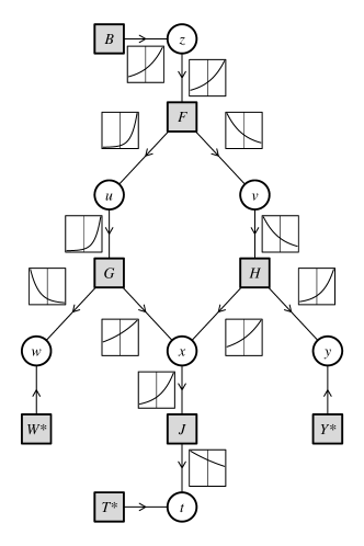
Figure 3: Lifted example network, with messages

7 Behavior of the lifted model

We are now interested in understanding the behavior of belief propagation on the lifted model. This behavior is specified to a great extent by the topological structure of the probabilistic network, which inherits certain properties from the fact that it derives from a function network. Each factor was originally a function with one or more input variables and only one output, and with each variable occurring as the output of at most one function. Therefore although there is a loop in the network, the network’s structure is not entirely general, and interactions between messages are channeled in such a way that certain invariants are maintained by the message updates. In addition to the distinction defined earlier between variable-factor and factor-variable messages, it is possible to assign an “upwards” or “downwards” direction to each message. We find that when running loopy belief propagation on a network that was produced by our lifting transformation, messages propagating upwards through the network are delta functions, but the downward messages can take an arbitrary form and are not converted into delta functions by any of the upward messages. When the algorithm converges, the posteriors at each variable node are delta functions centered at the value of the variable in the original function network computation, but the downward messages are nevertheless able to encode additional information from which the values of derivatives may be obtained.

To see why the upward messages are allowed to take a separate form from the downward messages, note that each variable has only one downward message leaving it, towards the factor that it represents the output of, and that this message is calculated only as the product of other downward messages coming from factors for which it had served as an input. Thus, although the product of any function with a delta function is another delta function, no delta functions enter into the product when downward messages are updated according to the variable$\to$factor message updates (equation 20).

The first downward message in the example network comes from the Boltzmann prior $B$:

$$m_{(B,z)}(z)=e^{z}$$ (24)

This is propagated unchanged from $z$ to $F$:

$$m_{(z,F)}(z)=e^{z}$$ (25)

We next calculate the message from $F$ to $U$:

$$m_{(F,u)}(u)=\int F(u,v,z)m_{(z,F)}(z)m_{(v,F)}(v)\mathrm{d}z\mathrm{d}v$$ (26)

Now $m_{(v,F)}(v)$ is an upward message and therefore a delta function, $\delta(v-v^{*})$. Substituting $F$ according to our lifting, we have

$$m_{(F,u)}(u)$$ (27)

$$=\int\delta(z-f(u,v))m_{(z,F)}(z)\delta(v-v^{*})\mathrm{d}v\mathrm{d}z$$ (28)

$$=m_{(z,F)}(f(u,v^{*}))$$ (29)

$$=\exp(f(u,v^{*}))$$ (30)

This is propagated without change to $G$, the only other neighbor of $u$:

$$m_{(u,G)}(u)=\exp(f(u,v^{*}))$$ (31)

Similarly we have

$$m_{(v,H)}(v)=m_{(F,v)}(v)=\exp(f(u^{*},v))$$ (32)

Similarly to the message from $F$ to $u$, the message from $G$ to $x$ must incorporate the upward message $m_{(w,G)}(w)$, which is a delta function $\delta(w-w^{*})$:

$$m_{(G,x)}(x)$$ (33)

$$=\int\delta(u-g(w,x))m_{(u,G)}(u)\delta(w-w^{*})\mathrm{d}u\mathrm{d}w$$ (34)

$$=m_{(u,G)}(g(w^{*},x))$$ (35)

$$=\exp\Bigl{(}f(g(w^{*},x),v^{*})\Bigr{)}$$ (36)

And we see that, correspondingly for $H$,

$$m_{(H,x)}(x)=\exp\Bigr{(}f(u^{*},h(x,y^{*}))\Bigl{)}$$ (37)

The message from $x$ to $J$ is simply the product of these two messages:

$$m_{(x,J)}(x)=\exp\Bigl{(}f(g(w^{*},x),v^{*})+f(u^{*},h(x,y^{*}))\Bigr{)}$$ (38)

Notice that

$$\frac{\mathrm{d}}{\mathrm{d}x}\log m_{(x,J)}(x)={\partial f\over\partial u}\frac{\mathrm{d}u}{\mathrm{d}x}+{\partial f\over\partial v}\frac{\mathrm{d}v}{\mathrm{d}x}=\frac{\mathrm{d}f}{\mathrm{d}x}$$ (39)

when evaluated at $x=x^{*}$ (and with $w=w^{*}$ and so on) which gives $\frac{\mathrm{d}f}{\mathrm{d}x}$ according to the chain rule. The relationship only holds when the derivative is evaluated at $x=x^{*}$, because $u^{*}$ and $v^{*}$ depend on $x^{*}$, and they appear as constants in the two terms.

It remains to show that the relationship of equation 39 holds more generally. Setting aside the example network, let us assume we are given an arbitrary function network and its lifted counterpart, a probabilistic network on which we have executed belief propagation. We want to establish two invariants which hold for the messages in the network. These invariants apply to downward messages of both types and relate them to the variable adjoints, which is to say the derivatives of an objective variable, $z$, with respect to each variable.

Theorem 1.

The following invariant holds for the downward message from any variable $x$ to the factor $F$ adjacently below it:

$$\left.\frac{\mathrm{d}}{\mathrm{d}x}\right|_{x=x^{*}}\log m_{(x,F)}(x)=\frac{\mathrm{d}z}{\mathrm{d}x}$$ (a)

And the following invariant holds for the downward message from a factor $F$ with output $y$ to one of its neighboring (input) variables, $x$:

$$\left.\frac{\mathrm{d}}{\mathrm{d}x}\right|_{x=x^{*}}\log m_{(F,x)}(x)=\frac{\mathrm{d}z}{\mathrm{d}y}\left({\partial y\over\partial x}\equiv{\partial f\over\partial x}\right)$$ (b)

We prove invariants (a) and (b) using induction, by assuming that they already hold for all the downward-directed messages above the current edge in the network, and expanding the current message using the message update rules of equations 19 and 20. After substituting equation 20 into invariant (a), we get

$$\frac{\mathrm{d}}{\mathrm{d}x}\log\left(m_{(x,F)}(x)=\prod_{G\succ x}m_{(G,x)}(x)\right)$$ (40)

where $G\succ x$ represents any factor $G$ above the variable $x$ in the network. Since $x$ must be the output node of $F$, this product iterates over all the neighbors of $x$ not equal to $F$, as specified by the message update rule. This becomes

$$\frac{\mathrm{d}}{\mathrm{d}x}\log\prod_{G\succ x}m_{(G,x)}(x) =\sum_{G\succ x}\left(\frac{\mathrm{d}}{\mathrm{d}x}\log m_{(G,x)}(x)\right)$$ (41)

$$=\sum_{G\succ x}\frac{\mathrm{d}z}{\mathrm{d}g}{\partial g\over\partial x}=\frac{\mathrm{d}z}{\mathrm{d}x}$$ (42)

the second equality following from the induction hypothesis and invariant (b). The lower-case $g$ stands for the function encoded by the factor $G$ and its output node. This summation is $\frac{\mathrm{d}z}{\mathrm{d}x}$ by the chain rule, which establishes invariant (a) for the message from $x$ to its child $F$.

To prove the second invariant, we substitute equation 19 into (b), which is to say

$$m_{(F,x)}(x)=\int \delta\left(\hat{f}-f(x,\{y\})\right)$$ (43)

$$m_{(\hat{f},F)}(\hat{f})\prod_{y}m_{(y,F)}(y)\mathrm{d}\hat{f}\mathrm{d}\{y\}$$ (44)

where $\hat{f}$ signifies the output variable associated with the function $f$, and $y$ represents all the inputs of $f$ except $x$. As with equation 28 above (in our analysis of the example model), the messages $m_{(y,F)}(y)$ are all delta functions, so the substitution becomes

$$\frac{\mathrm{d}}{\mathrm{d}x}\log \ m_{(F,x)}(x)=\frac{\mathrm{d}}{\mathrm{d}x}\log m_{(\hat{f},F)}(f(x,\{y^{*}\}))$$ (45)

$$=\left(\frac{\mathrm{d}}{\mathrm{d}\hat{f}}\log m_{(\hat{f},F)}(\hat{f})\right){\partial f\over\partial x}=\frac{\mathrm{d}z}{\mathrm{d}f}{\partial f\over\partial x}$$ (46)

where the last equality follows from the induction hypothesis and invariant (a).

We must finally prove the “base case” of the induction, namely that invariant (a) holds for the message from $z$ to the function node $F$ directly below it. Since the only other neighbor of $z$ is the Boltzmann factor $B$, this message is equal to the message from $B$ to $z$:

$$m_{(z,F)}(z)=m_{(B,z)}(z)=e^{z}$$ (47)

Invariant (a) then becomes

$$\left.\frac{\mathrm{d}}{\mathrm{d}z}\right|_{z=z^{*}}\log\left(m_{(z,F)}(z)=e^{z}\right)=\frac{\mathrm{d}}{\mathrm{d}z}\log e^{z}=1=\frac{\mathrm{d}z}{\mathrm{d}z}$$ (48)

and so it is satisfied for the base case. This completes the proof by induction.

We have described running belief propagation on a network where the independent variables are assigned delta function priors:

$$X^{*}(x)=\delta(x-x^{*})$$ (49)

In the case where these delta functions are approximated using a more general distribution such as a narrow Gaussian, it may be more useful to estimate the adjoints of our variables using a form of invariant (a) that does not depend on choosing a specific value $x^{*}$ at which to evaluate the derivative.

Corollary 1.

$$\frac{\mathrm{d}z}{\mathrm{d}x}=-\int\left({\partial\over\partial x}X^{*}(x)\right)\log m_{(x,X^{*})}(x)\mathrm{d}x$$ (50)

For the case of delta functions, this is equivalent to invariant (a) by analogy to the following integration by parts identity:

$$\int\left({\partial\over\partial x}\delta(x)\right)f(x)\mathrm{d}x=-{\partial f\over\partial x}(0)$$ (51)

But when $X^{*}$ is a Gaussian, for example, the above expression 50 for $\frac{\mathrm{d}z}{\mathrm{d}x}$ is equivalent to a kind of smoothed numerical differentiation.

Our proof by induction makes it clear that as with backpropagation, the converged belief propagation messages in our model can be calculated in a single forward and single backward pass over the network.

8 Conclusions

8.1 Motivation

Most papers in machine learning seek to introduce a new computer algorithm to the field. The purpose of this paper is rather to shed light on a connection between two well-established algorithms, to provide groundwork for a better theoretical understanding of both algorithms, and to eliminate some of the mystery surrounding them for students.

Belief propagation and backpropagation apply to different classes of input model. Belief propagation applies to probabilistic models and is used in domains where there is a need to model uncertainty directly, and backpropagation applies to deterministic models, where it is used to provide gradients to support the fitting of such models to data. Because all real-world data contains some measure of uncertainty, there is considerable overlap between these two domains, and it could be said that any essential difference between them is only a matter of engineering philosophy; based on the engineer’s decision about whether to model uncertainty directly or indirectly, and at which level of the system to do so [33, 34].

There has been recent interest in extensions of backpropagation that incorporate uncertainty more directly into the algorithm; some of these, such as stochastic gradient descent [35] or drop-out [36], apply backpropagation to inputs which change at random; others, such as probabilistic backpropagation [37], extend backpropagation by replacing deterministic quantities with probabilistic representations of the same quantities, somewhat related to the “lifting” we refer to in this paper. We hope that it would be possible to assist these investigations by clarifying the mathematical relationship between backpropagation and belief propagation.

The problem of characterizing the behavior of belief propagation on a lifted function network whose inputs have been initialized with distributions other than delta functions remains an open question. In this case, we can expect in general that the converged messages will not produce exact posteriors and will not lead to exact adjoints being calculated, because the downward messages will have the effect of slightly changing the variable locations specified in the upward messages (figure 4) and these effects will be compounded as the messages propagate around loops. We do not know whether a loop-corrected form of belief propagation would be necessary to make this more general scenario useful.

Figure 4: A Gaussian message being shifted to the right after multiplication by an exponential

However, before learning the inputs to a function network using gradient descent, the precise value of the input variables is in general unknown. Being able to make this uncertainty explicit at a more basic level, by running some form of backpropagation on a “lifted” probabilistic version of the network, with inputs that are not delta functions, could be desirable for a number of reasons, for example because it allows the convergence rate of the input variables to be reflected in their posterior distributions, or because it allows some of the input variables to be specified with less certainty than others, which could provide an evolving indicator of where the training algorithm should focus its attention.

Readers who are interested in probabilistic approaches to the problem of training “neural networks” could start with David MacKay’s thesis [38] which proposes approximations that could be used to model uncertainty at the level of variables in the network. Extensions to this idea are explored in for example [39] and [40]; more recently, [41] points out that by replacing backpropagation with message passing, it becomes easier to train networks that have discrete weights, which can be useful for hardware-based network implementations with limited numerical precision. “Probabilistic backpropagation” [37] is the name given to an approach that combines a forward pass that approximates the distribution at each network node as a Gaussian, with a backwards pass that backpropagates adjoints of these distribution parameters. Experiments show that the method compares favorably with plain backpropagation and with Hamiltonian Monte-Carlo, a probabilistic training method based on sampling [42], although there appear to be many details in the implementation. Our paper is less concerned with experimental results, and more concerned with making a sea of different ideas more navigable by pointing out some overlooked connections that exist within it.

Belief propagation and backpropagation are both useful for analyzing large models because they have the same time complexity as running the model itself. Like strict (non-loopy) belief propagation, backpropagation is a dynamic programming algorithm that requires only two passes over the input network, the first pass serving to compute the value of the objective or output variable, and the second pass serving to compute the derivatives. Loopy belief propagation, on the other hand, exchanges numerical messages locally on the network for some usually small number of iterations, typically until the messages converge; for error-correcting codes and certain other applications, convergence is fast enough that the algorithm does not add significant time complexity [12, 11, 43, 44]. While belief propagation and backpropagation both distinguish between input and output variables, loopy belief propagation requires no such distinction to be made.

Framing an algorithm in terms of locally-exchanged messages can be useful for distributing it across multiple computers, and there may be some value derived from being able to rethink backpropagation in terms of iterative local message-passing. Another contribution of this paper is to show that by placing backpropagation in the framework of loopy belief propagation, the input-output relationships of backpropagation become part of the messages rather than being hard-coded through the functions of the network, and the original function network can be inverted with respect to one of the input variables, simply by moving the Boltzmann prior onto this variable while leaving the rest of the network unchanged.

8.2 Generality

It is desirable to point out that the form of the “lifting” of a function network to a probabilistic network which we describe here is a straightforward requirement of the problem of converting from one class of inputs to the other. The “Dirac delta function” is a well-understood formalism for specifying a probability distribution that takes only a single value, and it is used to lift both variables and functions into the domain of probabilities.

The use of the Boltzmann distribution is motivated as follows: backpropagation is most commonly used to solve optimization problems; the most natural way of converting an optimization problem to a probabilistic inference problem is to place a Boltzmann distribution over the objective: $p(E)\propto\exp{E\over kT}$, where $E$ is the objective or output variable of the function network, and $kT$ is a constant specifying the tightness of the distribution around the optimum. This distribution has its origins in thermodynamics, where it describes the distribution over the states of a system with energy $E$ and temperature $T$ [45]. Also called the Gibbs measure in mathematical contexts, the Boltzmann distribution has widespread use in machine learning, for example in stochastic neural networks, see for example the “Boltzmann machine” [46, 47]; and arises almost universally in probability theory in a less recognizable form, the exponential family model, which appears whenever data consist of exchangeable observations [48].

There are a few hurdles to overcome in attempting to unify belief propagation and backpropagation. The first is that the domains of each algorithm are different, one being probabilistic and the other being deterministic. This is addressed by our “lifting” transformation, but the transformation produces models that are considered less tractable than a typical input to belief propagation: first of all, a typical lifted function network will contain many loops; and secondly, a function network operates on real-valued rather than discrete variables. Computing the message updates of belief propagation on the lifted network requires some difficult modeling decisions: how to represent distributions over real variables, whether to represent delta functions specially or as a limit of narrow Gaussians, how to perform the numerical integration required by the message updates, and how to represent the Boltzmann distribution and other messages which may be unnormalizable. All of these hurdles can be surmounted in various ways. There is a relatively long history of the successful use of belief propagation and related message-passing algorithms to perform efficient probabilistic inference in real-valued probability networks, see for example “assumed density filtering” and “expectation propagation” [49].

Finally, this work has relevance to researchers seeking to invent novel ways to improve the training phase of models based on function networks, which are seeing increasingly widespread application in computer science. Rather than changing the structure or mathematical relationships of the network to make it behave more tractably under a backpropagation-based training method, one could instead consider tuning its independent variables by applying belief propagation (or one of its many extensions) to a lifted, probabilistic, version of the network where it is possible to reason about uncertainty more directly.

To this end, it would seem helpful to observe that the original backpropagation algorithm is recovered exactly by loopy belief propagation in the case where the network is initialized with delta functions, just as it has often been helpful in the analysis of loopy belief propagation on general probabilistic networks to observe that the algorithm is exact in the case where the input network is a tree.

References

- [1] Isaac Newton. Philosophiæ Naturalis Principia Mathematica. Royal Society Press, 1687.
- [2] G.W. Leibniz. The Early Mathematical Manuscripts of Leibniz. The Open Court Publishing Company, 1920.
- [3] H.A. Bethe. Statistical Theory of Superlattices. Proceedings of the Royal Society of London. Series A, Mathematical and Physical Sciences, 150(871):552–575, 1935.
- [4] J.L. Lagrange. Théorie des fonctions analytiques. Courcier, 1797.
- [5] David E. Rumelhart, Geoffrey E. Hinton, and Ronald J. Williams. Learning representations by back-propagating errors. Nature, 323(6088):533–536, 1986.
- [6] T. Bayes. An Essay towards Solving a Problem in the Doctrine of Chances. By the Late Rev. Mr. Bayes, F. R. S. Communicated by Mr. Price, in a Letter to John Canton, A. M. F. R. S. Philosophical Transactions of the Royal Society of London, 53:370–418, 1763.
- [7] P.S. Laplace. Théorie analytique des probabilités. Courcier, 1812.
- [8] Judea Pearl. Probabilistic Reasoning in Intelligent Systems: Networks of Plausible Inference. Morgan Kaufmann, 1988.
- [9] Brendan J. Frey, Ralf Koetter, and Nemanja Petrovic. Very loopy belief propagation for unwrapping phase images. Advances in Neural Information Processing Systems, 14, 2001.
- [10] F.R. Kschischang, B.J. Frey, and H.A. Loeliger. Factor graphs and the sum-product algorithm. IEEE Transactions on information theory, 47(2):498–519, 2001.
- [11] N. Wiberg, H.A. Loeliger, and R. Kotter. Codes and iterative decoding on general graphs. European Transactions on telecommunications, 6(5):513–525, 1995.
- [12] David J.C. MacKay and Radford M. Neal. Good codes based on very sparse matrices. In IMA International Conference on Cryptography and Coding, pages 100–111. Springer, 1995.
- [13] Alexander T. Ihler, John W. Fisher III, Alan S. Willsky, and David Maxwell Chickering. Loopy belief propagation: convergence and effects of message errors. Journal of Machine Learning Research, 6(5), 2005.
- [14] Kyomin Jung and Devavrat Shah. Inference in binary pair-wise markov random fields through self-avoiding walks. Preprint on http://arxiv. org/abs/cs. AI/0610111v2, 2006.
- [15] M. Chertkov and V.Y. Chernyak. Loop series for discrete statistical models on graphs. Journal of Statistical Mechanics: Theory and Experiment, 2006, 2006.
- [16] Yusuke Watanabe and Kenji Fukumizu. Loop series expansion with propagation diagrams. Journal of Physics A: Mathematical and Theoretical, 42(4):045001, 2008.
- [17] M.J. Wainwright, T.S. Jaakkola, and A.S. Willsky. Tree-reweighted belief propagation algorithms and approximate ML estimation by pseudomoment matching. In Workshop on Artificial Intelligence and Statistics, volume 21, 2003.
- [18] J.M. Mooij, B. Wemmenhove, H.J. Kappen, and T. Rizzo. Loop corrected belief propagation. In Proceedings of the Eleventh International Conference on Artificial Intelligence and Statistics, 2007.
- [19] Oleg Kiselyov and Chung-chieh Shan. Embedded probabilistic programming. In IFIP Working Conference on Domain-Specific Languages, pages 360–384. Springer, 2009.
- [20] Ralf Hinze. Lifting operators and laws, 2010.
- [21] David Poole. First-order probabilistic inference. In IJCAI, volume 3, pages 985–991, 2003.
- [22] Rodrigo de Salvo Braz, Eyal Amir, and Dan Roth. Lifted first-order probabilistic inference. Statistical relational learning, page 433, 2007.
- [23] Bratin Saha and Zhong Shao. Optimal type lifting. In International workshop on types in compilation, pages 156–177. Springer, 1998.
- [24] Alexandra Ionescu Tulcea and Cassius Ionescu Tulcea. On the lifting property. Technical report, Yale Univ Dept of Mathematics, 1961.
- [25] Ludwig Boltzmann. Über die mechanische Bedeutung des zweiten Hauptsatzes der Wärmetheorie. Staatsdruckerei, 1866.
- [26] Ludwig Boltzmann. Weitere studien über das wärmegleichgewicht unter gasmolekülen (1872). In Kinetische Theorie II, pages 115–225. Springer, 1970.
- [27] Atilim Gunes Baydin, Barak A. Pearlmutter, Alexey Andreyevich Radul, and Jeffrey Mark Siskind. Automatic differentiation in machine learning: a survey. Journal of Marchine Learning Research, 18:1–43, 2018.
- [28] Jerrold E. Marsden, Anthony J. Tromba, and Alan Weinstein. Basic multivariable calculus. Springer, 1993.
- [29] Paul Adrien Maurice Dirac. The principles of quantum mechanics. Oxford university press, 1981.
- [30] Leonard E. Baum and Ted Petrie. Statistical inference for probabilistic functions of finite state markov chains. The annals of mathematical statistics, 37(6):1554–1563, 1966.
- [31] X.D. Huang, Y. Ariki, and M.A. Jack. Hidden Markov Models for Speech Recognition. Edinburgh University Press, 1991.
- [32] R. E. Kalman. A New Approach to Linear Filtering and Prediction Problems. Journal of Basic Engineering, 82(1):35–45, 03 1960.
- [33] Edwin T. Jaynes. Probability theory: The logic of science. Cambridge university press, 2003.
- [34] Kevin P. Murphy. Machine learning: a probabilistic perspective. MIT press, 2012.
- [35] Jack Kiefer and Jacob Wolfowitz. Stochastic estimation of the maximum of a regression function. The Annals of Mathematical Statistics, pages 462–466, 1952.
- [36] Nitish Srivastava, Geoffrey Hinton, Alex Krizhevsky, Ilya Sutskever, and Ruslan Salakhutdinov. Dropout: A simple way to prevent neural networks from overfitting. Journal of Machine Learning Research, 15(56):1929–1958, 2014.
- [37] Jose Miguel Hernandez-Lobato and Ryan Adams. Probabilistic backpropagation for scalable learning of bayesian neural networks. In Francis Bach and David Blei, editors, Proceedings of the 32nd International Conference on Machine Learning, volume 37, pages 1861–1869, 07–09 Jul 2015.
- [38] David John Cameron Mackay. Bayesian methods for adaptive models. PhD thesis, California Institute of Technology, 1992.
- [39] Sara A Solla and Ole Winther. Optimal perceptron learning: an online bayesian approach. On-Line Learning in Neural Networks. Cambridge University Press, Cambridge, 1998.
- [40] Alfredo Braunstein and Riccardo Zecchina. Learning by message passing in networks of discrete synapses. Physical review letters, 96(3):030201, 2006.
- [41] Daniel Soudry, Itay Hubara, and Ron Meir. Expectation backpropagation: Parameter-free training of multilayer neural networks with continuous or discrete weights. Advances in neural information processing systems, 27, 2014.
- [42] Radford M Neal. Bayesian Learning for Neural Networks. PhD thesis, University of Toronto, 1995.
- [43] Tom Richardson. The geometry of turbo-decoding dynamics. IEEE Transactions on Information Theory, 46(1):9–23, 2000.
- [44] Kevin Murphy, Yair Weiss, and Michael I. Jordan. Loopy belief propagation for approximate inference: An empirical study. arXiv preprint arXiv:1301.6725, 2013.
- [45] Enrico Fermi. Thermodynamics. Blackie, 1936.
- [46] David Sherrington and Scott Kirkpatrick. Solvable model of a spin-glass. Physical Review Letters, 35:1792–1796, Dec 1975.
- [47] David Ackley, Geoffrey Hinton, and Terrence Sejnowsky. A learning algorithm for boltzmann machines. Cognitive Science, 1985.
- [48] M.J. Wainwright and M.I. Jordan. Graphical models, exponential families, and variational methods. New Directions in Statistical Signal Processing, 2003.
- [49] Tom Minka. A family of algorithms for approximate Bayesian inference. PhD thesis, MIT, 2001.