Short-range forces due to Lorentz-symmetry violation

Abstract

Complementing previous theoretical and experimental work, we explore new types of short-range modifications to Newtonian gravity arising from spacetime-symmetry breaking. The first non-perturbative, i.e., to all orders in coefficients for Lorentz-symmetry breaking, are constructed in the Newtonian limit. We make use of the generic symmetry-breaking terms modifying the gravity sector and examine the isotropic coefficient limit. The results show new kinds of force law corrections, going beyond the standard Yukawa parameterization. Further, there are ranges of the values of the coefficients that could make the resulting forces large compared to the Newtonian prediction at short distances. Experimental signals are discussed for typical test mass arrangements.

1 Introduction

Presently, the nature of gravity is still largely unknown on length scales less than micrometers. In fact, new types of forces many times stronger than the Newtonian gravitational force could exist on short length scales and still be consistent with current experimental limits [1]. Suggestions for hypothetical new forces that could modify gravity at short ranges abound in the literature [2, 3, 4, 5, 6, 7, 8]. In particular, miniscule but potentially detectable violations of fundamental symmetries underlying General Relativity (GR) can arise in a plethora of ways [9, 10, 11, 12, 13, 14, 15]. The breaking of local Lorentz symmetry, for instance, can modify gravity on short ranges while being consistent with longer range measurements [16, 17].

To categorize the phenomenology of spacetime symmetry breaking one needs a comprehensive test framework. Effective field theory (EFT) is a widely used tool for describing potentially detectable new physics [18]. EFT descriptions of spacetime-symmetry breaking, including local Lorentz symmetry breaking, are based on including the action of GR and a standard matter sector action [19]. To these basic pieces, are added a series of symmetry breaking terms that can be organized by number of derivatives, curvature, mass dimensions, and so on [20, 21, 22]. This approach has the advantage that one can in principle calculate the effect on some observable due to some symmetry breaking terms, which can then be compared with entirely different observables in different scenarios, for measurements of the same coefficients controlling the size of the effects. Other formalisms for testing symmetries in gravity are parametrized directly from the form of a GR observable [23, 24, 25], or are based on specific models of alternatives to GR [26, 27, 28, 29].

We will consider in this work modifications to the gravity sector that, contrary to standard GR, break local Lorentz symmetry and diffeomorphism symmetry explicitly or spontaneously. These spacetime symmetries can be thought of as gauge symmetries for gravity, and thus GR is a gauge theory of gravity with local Lorentz and diffeomorphism symmetries as the gauge symmetries, analogous to Standard Model physics based on gauge groups [30]. The subtle issue of the role of broken spacetime symmetries in the context of curved spacetime, particularly when assuming asymptotically flat scenarios or not, has been discussed at length elsewhere [22, 31, 32]. While we do not fully discuss these concepts and subtleties here, we shall refer to conventions and categories of transformations in these references as needed.

In the EFT approach taken here, we highlight comparison of short-range (SR) gravity tests with gravitational wave (GW) observations, thus comparing two tests “across the universe” for measuring the same quantities describing spacetime-symmetry breaking for gravity. In fact, we show certain rotational scalar coefficients that can be measured in GW tests can also be probed in SR tests. Further, there are some coefficients that cannot be completely disentangled with GW tests alone, but using also SR gravity tests could accomplish this.

In references [16] and [17] solutions for short-range gravity tests were found, but these used an approximation of leading order in the coefficients. We show here that exact, non-perturbative, solutions can reveal where other combinations of coefficients, not yet disentangled, can show up in experiment. As we are concerned in this paper with modifications to gravity that do not break the Weak-Equivalence Principle, we do not discuss WEP violations here. The connection between Lorentz violation and WEP has been discussed at length elsewhere [33, 34, 35, 36].

Since we examine non-perturbative solutions, the results in this work also touch on the nature of higher than second order derivatives in the action and how that might affect gravity. For this latter topic, we do not attempt a comprehensive investigation of these issues but simply note where results exhibit behavior expected of such models [37, 38, 39], and how they might be consistent with perturbative approaches.

The paper is organized as follows. In section 2, we review two commonly used EFT schemes for the description of spacetime symmetry breaking in gravity and we discuss prior results in short-range gravity signals for Lorentz violation. In section 3, we explore non-perturbative solutions with a special case model to identify key features. Following this, we go on to solve the general EFT framework in the static, isotropic coefficient limit. Features of the solutions are discussed and explained with several plots. We discuss attempting exact solutions with anistropic coefficients in section 4, and compare to perturbative methods. For Section 5, we apply the theoretical results to simulate the signal of the gravitational field above a flat plate of mass, and comment on the experimental signatures. A summary and outlook is provided in section 6. Finally, in the appendix we include a review of relevant differential equations, the details of the tensor analysis for isotropic coefficients used, and special cases of the SR gravity solutions. In this work, we assume 4 dimensional spacetime with metric signature $-+++$ and units where $\hbar=c=1$. Latin letters are used for 3 dimensional space, and Greek letters for spacetime indices.

2 Background theory

2.1 Action and field equations

One can work with an observer covariant EFT expansion or an action designed for weak-field applications, the latter formulated in a quadratic action expansion. The two approaches are overlapping descriptions of physics beyond GR and the SM when spacetime symmetries are broken. We display both approaches here, to emphasize recent points of view in the literature, and because we use them in this work.

It is a basic premise that in the EFT context, a breaking of spacetime symmetries is indicated by the presence of a background tensor field of some kind that couples to matter or gravity or both [9, 19, 20]. The details and subtleties of this premise have been discussed at length elsewhere [22, 31, 32]. Suffice it to say here that the EFT maintains coordinate invariance of physics (observer invariance) while the action may not be invariant under symmetry transformations of localized field configurations (particle transformations). The latter violation is due to the presence of the background tensor fields, which remain fixed under such transformations.

The observer covariant expansion has a Lagrange density that takes the form of a series of terms:

$${\cal L} = {\textstyle{{\sqrt{-g}}\over{2\kappa}}}\big{(}R+k^{(4)}_{\alpha\beta\gamma\delta}R^{\alpha\beta\gamma\delta}+k^{(5)}_{\alpha\beta\gamma\delta\kappa}\nabla^{\kappa}R^{{\alpha\beta\gamma\delta}}$$ (1)

$$\phantom{space}+k^{(6)}_{\kappa\lambda\mu\nu{\alpha\beta\gamma\delta}}R^{\kappa\lambda\mu\nu}R^{{\alpha\beta\gamma\delta}}+...\big{)}+{\cal L}^{\prime}.$$

In this expression, the determinant of the metric is $\sqrt{-g}$, $R^{\alpha\beta\gamma\delta}$ is the Riemann curvature tensor, $R$ is the Ricci scalar, and $k^{(4)}_{\alpha\beta\gamma\delta}$, $k^{(5)}_{\alpha\beta\gamma\delta\kappa}$, and $k^{(6)}_{\kappa\lambda\mu\nu{\alpha\beta\gamma\delta}}$ are the coefficients controlling the degree of symmetry breaking [22, 16]. The coupling is $\kappa=8\pi G_{N}$, where $G_{N}$ is the gravitational constant. The first term is the Einstein-Hilbert lagrange density, while the remaining terms are the symmetry-breaking terms. Note that additional terms for the coefficients can be included in ${\cal L}^{\prime}$. For instance, a general expansion for such terms exists, for the case of a two-tensor $s_{\mu\nu}\propto k^{(4)\alpha}_{\phantom{(4)\alpha}\mu\alpha\nu}$, and takes the form

$${\cal L}^{\prime} = {{\sqrt{-g}}\over{2\kappa}}\Big{[}a_{3}{\textstyle{{1}\over{2}}}(\nabla_{\mu}s_{\nu\lambda})(\nabla^{\mu}s^{\nu\lambda})+a_{4}{\textstyle{{1}\over{2}}}(\nabla_{\mu}s^{\mu\lambda})(\nabla_{\lambda}s^{\beta}_{\phantom{\beta}\beta})$$ (2)

$$\phantom{space}+...+a_{7}s_{\mu\nu}s_{\kappa\lambda}R^{\mu\kappa\nu\lambda}+a_{8}s_{\mu\nu}s^{\mu}_{\phantom{\mu}\lambda}R^{\nu\lambda}+...\Big{]},$$

which can be viewed as terms of second order in the coefficients or as dynamical terms [40, 32]. Alternatives to (2) can adopt the explicit symmetry breaking scenario, where the coefficients in (1) are given a priori, this latter possibility given emphasis more recently [41, 42, 43, 44].

An alternative overlapping approach, the quadratic action approach, assumes an expansion around flat spacetime $\eta_{\mu\nu}$, of the standard form

$$g_{\mu\nu}=\eta_{\mu\nu}+h_{\mu\nu}.$$ (3)

We examine the quadratic action [45, 46] in the limit that maintains the usual linearized gauge invariance of GR: $h_{\mu\nu}\rightarrow h_{\mu\nu}-\partial_{\mu}\xi_{\nu}-\partial_{\nu}\xi_{\mu}$. The Lagrange density for this approach takes the form

$${\cal L}=-{\textstyle{{1}\over{4\kappa}}}h^{\alpha\beta}G_{\alpha\beta}+{\textstyle{{1}\over{8\kappa}}}h_{\mu\nu}(\hat{s}^{\mu\rho\nu\sigma}+\hat{q}^{\mu\rho\nu\sigma}+\hat{k}^{\mu\rho\nu\sigma})h_{\rho\sigma},$$ (4)

where $G_{\alpha\beta}$ is the linearized Einstein tensor. The “hat” operators are built from background coefficients for spacetime-symmetry breaking and partial derivatives. The three types appearing in (4) are given by,

$$\hat{s}^{\mu\rho\nu\sigma} = s^{(d)\mu\rho\epsilon_{1}\nu\sigma\epsilon_{2}...\epsilon_{d-2}}\partial_{\epsilon_{1}}...\partial_{\epsilon_{d-2}},$$

$$\hat{q}^{\mu\rho\nu\sigma} = q^{(d)\mu\rho\epsilon_{1}\nu\epsilon_{2}\sigma\epsilon_{3}...\epsilon_{d-2}}\partial_{\epsilon_{1}}...\partial_{\epsilon_{d-2}},$$

$$\hat{k}^{\mu\nu\rho\sigma} = k^{(d)\mu\epsilon_{1}\nu\epsilon_{2}\rho\epsilon_{3}\sigma\epsilon_{4}...\epsilon_{d-2}}\partial_{\epsilon_{1}}...\partial_{\epsilon_{d-2}}.$$ (5)

While the expansions in (5) appear similar for the three types of coefficients, the $s$, $q$, and $k$ in fact differ by symmetry and tensor properties. The detailed tensor properties of these terms are described in the Young Tableau of Table 1 of Ref. [45], (some samples are included in appendix (75)). In particular, $\hat{s}^{\mu\rho\nu\sigma}$ is anti-symmetric in the pairs of indices $\mu\rho$ and $\nu\sigma$, while $\hat{q}^{\mu\rho\nu\sigma}$ is anti-symmetric in $\mu\rho$ and symmetric in $\nu\sigma$, and finally $\hat{k}^{\mu\nu\rho\sigma}$ is symmetric in the pairs of indices $\mu\rho$ and $\nu\sigma$. In terms of discrete spacetime symmetries, The $\hat{s}$ operators have even CPT symmetry and mass dimension $d\geq 4$; $\hat{q}$ operators have odd CPT and mass dimension $d\geq 5$; $\hat{k}$ operators have even CPT and mass dimension $d\geq 6$.

The phenomenology of the terms in (1) and (4) has been studied in a number of works. Observable effects in weak-field gravity tests have been established for a subset of the possible terms [47, 48, 16] and some work has been done on strong-field gravity regimes like cosmology [49, 42, 50, 51]. Effects on gravitational waves have been studied, showing that dispersion and birefringence occur generically as a result of CPT and Lorentz violation [45]. Analysis has been performed in tests such as lunar laser ranging [52], gravimetry [53], pulsars [54], and using the catalog of GW events [55, 56, 57, 58, 59]. An exhaustive list of up to date experimental limits and papers on gravity sector coefficients can be found in [60].

On the theory side, explicit local Lorentz and diffeomorphism symmetry cases have been explored various contexts. A “3+1” formulation of the EFT framework has been explored in Refs. [42, 43, 61]. Extensive work has been completed mapping out the approach to explicit symmetry breaking with Finsler geometry [62, 63, 64, 65]. Other work includes much attention to vector and tensor models of spontaneous symmetry breaking [26, 66, 67, 68, 27, 69, 70] and how these models can be matched to the EFT expansion above [71, 72, 42, 44]. More recently, black hole solutions have been studied [73, 74, 75]. Also, the systematic construction of dynamical terms for the spontaneous symmetry breaking scenario, like in (2), has been undertaken in the gravity sector [40]. Finally we note some recent theoretical work has identified general properties of backgrounds in effective field theory [32], and new types of tests are possible that search for non-Riemann geometry [76].

Of the two approaches identified above, the latter, equation (4), is appropriate for short-range gravity tests. Such tests involve weak gravitational fields in the Earth laboratory setting, thus the typical size of components of $h_{\mu\nu}$ are much less than unity, in cartesian coordinates. Furthermore, to keep a reasonable scope we will truncate the series (5) to mass dimensions $4$, $5$, and $6$.

Any study of actions with higher than second order derivatives is subject to well-known results, such as Ostragradsky instabilities [39]. In the present paper, while the test framework (4) is viewed perturbatively, with the higher derivative terms as small corrections [77], our discussion of solutions beyond leading order in coefficients will overlap with features in higher derivative models. Some features are discussed in our results in Section 3 and Section 4.

2.2 Prior short-range gravity results

In references [16] and [17], Lorentz-symmetry breaking solutions for short-range gravity tests were found using an approximation of first order in the coefficients. We summarize these results briefly here for comparison. Assuming a static matter source and using the framework of (4), one solves the field equations perturbatively assuming any modifications to the field equations from symmetry-breaking terms are small [47, 16, 17]. The leading order modified Newtonian potential from a point mass $m$ at the origin can be written in terms of Newton spherical coefficients $k_{jm}^{N(d)lab}$ as a series

$$U={{G_{N}m}\over{r}}+\sum_{djm}{{G_{N}m}\over{r^{d-3}}}\,Y_{jm}(\theta,\phi)k_{jm}^{N(d)lab},$$ (6)

where the angular dependence $\theta,\phi$ in the spherical harmomics $Y_{jm}(\theta,\phi)$ pertains to the vector from the origin to the field point $\vec{r}=r(\sin\theta\cos\phi,\sin\theta\sin\phi,\cos\theta)$ and $r=|\vec{r}|$. The spherical coefficients $k_{jm}^{N(d)lab}$ are related to the coefficients in Eq. (5) as linear combinations, but the expressions are lengthy and omitted here, and relations between the dimension label $(d)$ and the allowed values of $j$ can be found in [17]. The superscript “lab” means that the coefficients are written in the laboratory coordinate system. Typically, the lab frame coefficients are re-expressed in terms of the Sun-centered Celestial Equatorial Frame coefficients using an observer Lorentz transformation, revealing harmonic time dependence [78, 79, 80].

The result in equation (6) has already been used for analysis in experiments [81, 82, 83, 84]. In fact, new experiments can be designed to maximize the type of anisotropic signal in (6) [83, 85, 86]. Recent result place limits on $14$ $k_{jm}^{N(6)}$ coefficients and $22$ $k_{jm}^{N(8)}$ coefficients at the $10^{-9}\,m^{2}$ and $10^{-12}\,m^{4}$ levels, respectively. However, the leading order approximation used for (6) makes searches in some short-range tests challenging, as some tests are designed to probe very small length scales at the cost of sensitivity to the Newtonian force from the test masses [87]. Such tests often lie outside the range of applicability of the result (6), which assumes the extra correction term to the Newtonian potential is smaller than the first term.

One other observation is that, with the exception of mass dimension $4$ coefficients, no rotational scalar coefficients, or isotropic coefficients show up in the result (6). In fact, it has been shown that one combination of isotropic coefficients does show up in the perturbative analysis, but only as contact term that vanishes outside of the matter distribution [16]. As we show below, a non-perturbative treatment reveals in more detail the role played by these coefficients.

3 Isotropic coefficients, Newtonian limit, nonperturbative

3.1 Special case model

We begin with a special case to illustrate the features of the solutions studied in this work. One particular model that contains the interesting features of exact short-range solutions is the following Lagrange density:

$${\cal L}={\textstyle{{1}\over{2\kappa}}}\sqrt{-g}\left(R+k_{\alpha\beta}R^{\alpha\beta}R\right),$$ (7)

which is a special case of (1). The second term is the non-standard one with the coefficients for Lorentz violation denoted $k_{\alpha\beta}$. These $10$ quantities have units of length squared or inverse mass squared in natural units.

The action in (7), yields the field equations in appendix (69), upon variation with respect to the full metric $g_{\mu\nu}$. In the linearized gravity limit, and assuming the coefficients $k_{\alpha\beta}$ have vanishing partials $\partial_{\alpha}k_{\beta\gamma}=0$, the field equations (69) become,

$$(G_{L})^{\mu\nu} = -{\textstyle{{1}\over{2}}}\eta^{\mu\nu}k_{\alpha\beta}\partial^{\alpha}\partial^{\beta}R_{L}-\eta^{\mu\nu}k_{\alpha\beta}\partial^{\gamma}\partial_{\gamma}(R_{L})^{\alpha\beta}+{\textstyle{{1}\over{2}}}k^{\nu\alpha}\partial_{\alpha}\partial^{\mu}R_{L}$$ (8)

$$+{\textstyle{{1}\over{2}}}k^{\mu\alpha}\partial_{\alpha}\partial^{\nu}R_{L}+k_{\alpha\beta}\partial^{\mu}\partial^{\nu}(R_{L})^{\alpha\beta}-{\textstyle{{1}\over{2}}}k^{\mu\nu}\partial^{\alpha}\partial_{\alpha}R_{L}+\kappa T^{\mu\nu},$$

where $T^{\mu\nu}$ is the matter stress-energy tensor. Note that in the linearized gravity case, indices are raised and lowered with $\eta_{\mu\nu}$, the linearized Ricci tensor is $(R_{L})_{\mu\nu}=(1/2)(\partial_{\mu}\partial^{\alpha}h_{\alpha\nu}+\partial_{\nu}\partial^{\alpha}h_{\alpha\mu}-\partial_{\alpha}\partial^{\alpha}h_{\mu\nu}-\partial_{\mu}\partial_{\nu}h^{\alpha}_{\phantom{\alpha}\alpha})$, $R_{L}=\partial^{\alpha}\partial^{\beta}h_{\alpha\beta}-\partial_{\alpha}\partial^{\alpha}h^{\beta}_{\phantom{\beta}\beta}$, and $(G_{L})^{\mu\nu}=(R_{L})^{\mu\nu}-(1/2)\eta^{\mu\nu}R_{L}$. The task is next to obtain a space and time component decomposition of these field equations (8).

If we further restrict attention to the static limit and only isotropic coefficients $k_{00}$ and $k_{jj}$, in a special coordinate system, we obtain the following coupled equations for the metric components $h_{00}$ and $h_{jj}$ (in harmonic gauge):

$$\nabla^{2}(h_{00}+h_{jj})-3({k_{00}}-{\textstyle{{1}\over{9}}}{k_{ll}})\nabla^{4}h_{00}+({k_{00}}-k_{ll})\nabla^{4}h_{jj} = -32\pi G_{N}\rho,$$

$$\nabla^{2}(3h_{00}+h_{jj})+4({k_{00}}-{\textstyle{{1}\over{3}}}k_{ll})\nabla^{4}h_{00}+{\textstyle{{8}\over{3}}}k_{ll}\nabla^{4}h_{jj} = 0.$$ (9)

Note that ${k_{ll}}-{k_{00}}=k_{\mu\nu}\eta^{\mu\nu}$ is a Lorentz invariant scalar combination. We have assumed a static pressure-less matter distribution so that only $T^{00}=\rho$ is nonzero in $T^{\mu\nu}$. We also find in this limit that the equation for $h_{0i}$ is simply Laplace’s equation:

$$\nabla^{2}h_{0i}=0.$$ (10)

For the remaining components of $h_{ij}$ it is advantageous to express the solution in terms of a traceless piece. By this we mean that if the equations for $h_{ij}$ are denoted ${\cal E}_{ij}=0$, the relevant projection is ${\cal E}_{ij}-(1/3)\delta_{ij}{\cal E}_{kk}$. This yields

$$\nabla^{2}(h_{ij}-{\textstyle{{1}\over{3}}}\delta_{ij}h_{kk})-2({k_{00}}-{\textstyle{{1}\over{3}}}{k_{ll}}){\cal D}_{ij}\nabla^{2}h_{00}-{\textstyle{{4}\over{3}}}{k_{ll}}{\cal D}_{ij}\nabla^{2}h_{kk}=0,$$ (11)

where ${\cal D}_{ij}=\partial_{i}\partial_{j}-{\textstyle{{1}\over{3}}}\delta_{ij}\nabla^{2}$ is a traceless operator. Evidently, if one can solve independently for $h_{00}$ and $h_{ll}$, then equation (11) can be viewed as an inhomogeneous equation for the traceless piece of $h_{ij}$ with source terms involving projections of $h_{00}$ and $h_{ll}$.

Our main focus is to solve the equations (9) for $h_{00}$ and $h_{jj}$, since $h_{00}$ is the metric component directly related to the Newtonian potential $U_{N}$ via $h_{00}=2U_{N}$. The solution can be found using standard methods of solving PDEs. We first discuss the construction of a Green function solution where we assume a point source $4\pi G_{N}\rho=\delta^{(3)}(\vec{r}-\vec{r}^{\prime})$. The point source solutions for $h_{00}$ and $h_{jj}$ are denoted ${\cal G}_{1}$ and ${\cal G}_{2}$.

Given the form of the solution to the equation with $\nabla^{2}$ and $\nabla^{4}$ in appendix (73), we propose the ansatz that the general solutions will take the form of the following functions of $R=|\vec{r}-\vec{r}^{\prime}|$:

$${\cal G}_{1}={1\over R}\left(A_{1}e^{-q_{1}R}+A_{2}e^{-q_{2}R}+A_{3}\right),$$

$${\cal G}_{2}={1\over R}\left(B_{1}e^{-q_{1}R}+B_{2}e^{-q_{2}R}+B_{3}\right),$$ (12)

Here the $A_{n}$’s and $B_{n}$’s are constants to be solved for as well as the $q_{1}$ and $q_{2}$. In constructing this solution we are assuming the boundary conditions such that the metric components go to zero far from the source, and we neglect any homogeneous solutions to (9). Insertion of (12) into the point source version of (9), followed by using the properties of functions of $R=|\vec{r}-\vec{r}^{\prime}|$, allows one to solve for the $8$ parameters $A_{1}$, $A_{2}$, $A_{3}$, $B_{1}$, $B_{2}$, $B_{3}$, $q_{1}$, and $q_{2}$ from $8$ resulting algebraic equations.

First, we find that for nontrivial solutions, both $q_{1}^{2}$ and $q_{2}^{2}$ must satisfy the quartic equation:

$$1+({k_{00}}-{\textstyle{{5}\over{3}}}{k_{ll}})q^{2}+({k_{00}}+{\textstyle{{1}\over{3}}}{k_{ll}})^{2}q^{4}=0.$$ (13)

The solutions to (13) can be obtained from the quadratic result,

$$q^{2}=u\pm v,$$ (14)

where $u$ and $v$ are given by:

$$u = {-({k_{00}}-{\textstyle{{5}\over{3}}}{k_{ll}})\over 2({k_{00}}+{\textstyle{{1}\over{3}}}{k_{ll}})^{2}},$$

$$v = {\sqrt{({k_{00}}-{\textstyle{{5}\over{3}}}{k_{ll}})^{2}-4({k_{00}}+{\textstyle{{1}\over{3}}}{k_{ll}})^{2}}\over 2({k_{00}}+{\textstyle{{1}\over{3}}}{k_{ll}})^{2}}$$ (15)

The four possible roots of the equation (13) can be obtained generally by taking the complex square roots of (14). The position of $z=q^{2}$ in the complex plane depends on the values of the coefficients ${k_{00}}$ and ${k_{ll}}$. Note that $u$ is real and $v$ can be real or complex. The values of the coefficients determine the properties of the $4$ possible roots $\{q=z^{1/2}=\pm(u\pm v)^{1/2}\}$. If $q$ is entirely real and positive, then the solutions in (12) will exhibit exponential damping in $R$ or short-range Yukawa-like behavior. The case where $q$ is negative and real will result in runaway exponential increase and is not physically viable. When $q$ has an imaginary piece or is entirely imaginary, the solution will have oscillations in $R$.

In what follows we assume the condition $q_{1}^{2}\neq q_{2}^{2}$. This condition ensures that the coefficients ${k_{00}}$ and ${k_{ll}}$ are treated a priori independent. This condition implies that in (14), $q_{1}^{2}$ takes one sign in the $\pm$, and $q_{2}^{2}$ takes the other sign. For this case we obtain the solutions for the Green function ${\cal G}_{1}$ as follows.

$${\cal G}_{1} = {1\over 2\pi R}-{1\over 4\pi}\left(1+{{k_{00}}+{\textstyle{{11}\over{3}}}{k_{ll}}\over\sqrt{({k_{00}}-{\textstyle{{5}\over{3}}}{k_{ll}})^{2}-4({k_{00}}+{\textstyle{{1}\over{3}}}{k_{ll}})^{2}}}\right){e^{-R/\lambda_{+}}\over R}$$ (16)

$$-{1\over 4\pi}\left(1-{{k_{00}}+{\textstyle{{11}\over{3}}}{k_{ll}}\over\sqrt{({k_{00}}-{\textstyle{{5}\over{3}}}{k_{ll}})^{2}-4({k_{00}}+{\textstyle{{1}\over{3}}}{k_{ll}})^{2}}}\right){e^{-R/\lambda_{-}}\over R},$$

where the $\lambda_{\pm}$ constants are defined by

$${1\over(\lambda_{\pm})^{2}}=u\pm v,$$ (17)

and they act like two distinct length scales.

We note the contrast of this result with previous results. First, unlike the Yukawa potential,

$$U_{Y}={{Gm}\over{r}}\left(1+\alpha e^{-r/\lambda}\right),$$ (18)

we have $2$ length scales in (17). Second, the amplitudes of the two terms vary depending on the values of the coefficients. In particular, we find that these amplitudes could take on large values for a narrow range of coefficient ratios ${k_{ll}}/{k_{00}}$, even if the coefficients themselves are small compared to the length scales probed. This is in contrast to standard assumptions of the smallness of Lorentz-violating effects. Note that the length scales would also be small, so such large Lorentz-breaking forces could escape detection in long-range tests, and this philosophy is along the lines of proposals for new short-range forces more generally.

To get an idea of the behavior of these solutions as the values of the coefficients change, in figure 1, we plot the potential $U=2{\cal G}_{1}$ for a point mass of unit strength as a function of ${k_{ll}}/{k_{00}}$ for several values of the distance $R$ (more specifically, the ratio of the distance $R$ to $\sqrt{k_{00}}$). This can be compared to the standard Newtonian potential which would be a horizontal line in the same graph. We clearly see a singular point in the ${k_{ll}}$, ${k_{00}}$ parameter space as the ${k_{ll}}/{k_{00}}$ approaches $-3/7$.

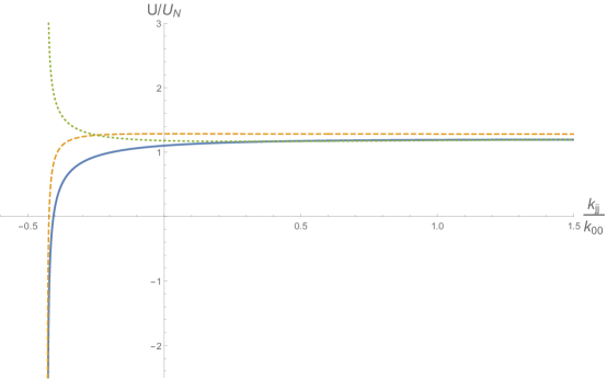
Figure 1: A plot of the ratio of the modified potential of equation (16) divided by the Newtonian potential for a unit mass at the origin. The horizontal axis is the coefficient ratio $k_{jj}/{k_{00}}$ while the solid curve, dashed curve, and dotted curves are the cases of different positions away from the point mass, $R=\sqrt{k_{00}}$, $R=3\sqrt{k_{00}}$, and $R=5\sqrt{k_{00}}$, respectively.

The solution obtained in (16) above agrees precisely with an alternative method, where one uses Fourier decomposition in momentum space, followed by contour integration. For practical evaluation over distributions of matter, such as those used in experiment, one would take the integral of the Green functions over the smooth matter distributions $\rho(\vec{r}^{\prime})$ as usual. Thus, since $h_{00}=2U$, the Newtonian potential is

$$U=2\pi G_{N}\int d^{3}r^{\prime}\rho(\vec{r}^{\prime}){\cal G}_{1}(\vec{r},\vec{r}^{\prime}).$$ (19)

3.2 General effective field theory case

Here we consider generalizing the solution of section 3.1. A more general treatment includes the quadratic Lagrange density of (4). First we examine the field equations for this approach, which are obtained from (4) by variation with respect to $h_{\mu\nu}$:

$$(G_{L})^{\mu\nu}+\delta M^{\mu\nu\rho\sigma}h_{\rho\sigma}=8\pi G_{N}T^{\mu\nu},$$ (20)

where we have adopted the notation of Ref. [17] with

$$\delta M^{\mu\nu\rho\sigma}h_{\rho\sigma} = -\Big{[}{\textstyle{{1}\over{4}}}(\hat{s}^{\mu\rho\nu\sigma}+\hat{s}^{\mu\sigma\nu\rho})+{\textstyle{{1}\over{2}}}\hat{k}^{\mu\nu\rho\sigma}$$ (21)

$$\phantom{+}+{\textstyle{{1}\over{8}}}(\hat{q}^{\mu\rho\nu\sigma}+\hat{q}^{\nu\rho\mu\sigma}+\hat{q}^{\mu\sigma\nu\rho}+\hat{q}^{\nu\sigma\mu\rho})\Big{]}h_{\rho\sigma}.$$

3.2.1 Determining the field equations

Next we will focus attention on mass dimension $d=6$ or less to keep the scope reasonable. Furthermore, as we are taking the static limit, as the prior section, only spatial derivatives appear. We will again choose to look at only isotropic coefficients, as these we expect to result in field equations we can solve exactly in analytic form, and to reveal the role of these coefficients in short-range gravity tests.

It is not exactly trivial to extract the isotropic coefficients in the expansions (5) but we outline the process here and leave most of the details for the appendix. Consider the $\mu=0,\nu=0$ component of (21), including terms up to mass dimension $6$. Tensor symmetry properties of the coefficients in (21) can be used to eliminate some contributions outright (see the Young Tableau in Table 1 of Ref. [45] and the appendix of this paper (75) ). For instance, antisymmetry of the indices yields ${\hat{s}}^{0000}=0={\hat{s}}^{000i}$ and ${\hat{q}}^{000i}=0$. The surviving contributions to the $00$ component of (21) are initially collected as

$$\delta M^{00\rho\sigma}h_{\rho\sigma} = -{\textstyle{{1}\over{2}}}k^{(6)0i0j0k0l}\partial_{ijkl}h_{00}$$ (22)

$$-\{{\textstyle{{1}\over{2}}}k^{(6)0j0k0lim}\partial_{jklm}+{\textstyle{{1}\over{4}}}q^{(5)0ij0k0l}\partial_{jkl}\}h_{0i}$$

$$-\{{\textstyle{{1}\over{2}}}[s^{(4)0ik0jl}\partial_{kl}+s^{(6)0ik0jlmn}\partial_{klmn}+k^{(6)0k0limjn}\partial_{klmn}]$$

$$\phantom{--}+{\textstyle{{1}\over{4}}}[q^{(5)0ik0ljm}+q^{(5)0jk0lim}]\partial_{klm}\}h_{ij}$$

where we make use of a short-hand ($\partial_{ijk...}=\partial_{i}\partial_{j}\partial_{k}...$) for multiple partials. Among the coefficients occurring in (22), those that are isotropic will be invariant under observer rotations $SO(3)$, and thus expressible in terms of rotational scalar contractions, the kronecker delta $\delta^{ij}$ and the levi-civita $\epsilon^{ijk}$.

As an example of how to decompose the terms in (22), consider the first term on the first line with the coefficients $k^{(6)0i0j0k0l}$, which has $ij$ and $kl$ index symmetry. This would lead us to the only available scalar contractions being $k^{(6)0i0i0j0j}$ and $k^{(6)0i0j0i0j}$. However, because the underlying tensor satisfies the cyclic identity $k^{(6)\mu\epsilon_{1}\nu\epsilon_{2}\rho\epsilon_{3}\sigma\epsilon_{4}}+k^{(6)\mu\epsilon_{1}\nu\epsilon_{3}\epsilon_{2}\rho\sigma\epsilon_{4}}+k^{(6)\mu\epsilon_{1}\nu\rho\epsilon_{2}\epsilon_{3}\sigma\epsilon_{4}}=0$, one can show that $k^{(6)0i0j0i0j}=k^{(6)0i0i0j0j}$. Therefore the $k^{(6)0i0j0k0l}$ coefficients, in the isotropic limit, must be proportional to combinations of kronecker deltas $\delta^{ij}\delta^{kl}+...$ and the one scalar $k^{(6)0i0i0j0j}$. Symmetry considerations lead us to

$$k^{(6)0i0j0k0l}={\textstyle{{1}\over{15}}}(\delta^{ij}\delta^{kl}+\delta^{ik}\delta^{jl}+\delta^{il}\delta^{jk})k^{(6)0m0m0n0n},$$ (23)

and thus

$$-{\textstyle{{1}\over{2}}}k^{(6)0i0j0k0l}\partial_{ijkl}h_{00}=-{\textstyle{{1}\over{10}}}k^{(6)0m0m0n0n}\nabla^{4}h_{00}.$$ (24)

which simplifies the first term in (22) to the desired form.

For the second line in (22), the coefficients $k^{(6)0j0k0lim}$ and $q^{(5)0ij0k0l}$ do not appear to have any scalar contractions due to the number of indices, or the symmetry properties. Nor can they be written in terms of purely $\delta_{ij}$ and $\epsilon_{ijk}$. We conclude their isotropic limit contribution vanishes:

$$-\{{\textstyle{{1}\over{2}}}k^{(6)0j0k0lim}\partial_{jklm}+{\textstyle{{1}\over{4}}}q^{(5)0ij0k0l}\partial_{jkl}\}h_{0i}\stackrel{{\scriptstyle\mathrm{iso}}}{{=}}0.$$ (25)

One proceeds along similar lines for the remaining terms in (22). The details are relegated to the appendix.

The final simplification to the isotropic coefficient case for (22) results in

$$\delta M^{00\rho\sigma}h_{\rho\sigma} = -{\textstyle{{1}\over{10}}}k^{(6)0m0m0n0n}\nabla^{4}h_{00}$$ (26)

$$+\{{\textstyle{{1}\over{12}}}s^{(4)0kl0kl}+{\textstyle{{1}\over{30}}}s^{(6)0kl0klmm}\nabla^{2}+{\textstyle{{1}\over{30}}}k^{(6)0k0klmlm}\nabla^{2}\}$$

$$\times(\partial_{i}\partial_{j}-\delta^{ij}\nabla^{2})h_{ij}.$$

Note the absence of the $h_{0i}$ components in this case. The remaining components of (21) $\mu=0,\nu=i$ and $\mu=i,\nu=j$ are worked out in the appendix. The equation for $h_{0i}$ decouples from the remaining components of $h_{\mu\nu}$ and we display below the coupled equations for the components $h_{00}$ and $h_{jj}$. As in the special case of the previous section, the off-diagonal components of $h_{ij}$ can be obtained from a traceless version of appendix (81), of secondary interest in this work.

To obtain the relevant differential equations we make the partial choice of gauge: $\partial_{j}h_{ij}=\partial_{i}(h_{jj}-h_{00})/2$. Furthermore, it will be convenient for solving the differential equations to work with the trace-reversed components $\bar{h}_{00}=(1/2)(h_{00}+h_{jj})$ and $\bar{h}_{jj}=(1/2)(3h_{00}-h_{jj})$. Also, since they can be probed with other tests [48], we disregard the mass dimension $4$ isotropic coefficients. With these choices and the results of the appendix, the two coupled equations are given by,

$$-{\textstyle{{1}\over{2}}}[\nabla^{2}+(k_{1}+k_{2})\nabla^{4}]\bar{h}_{00}-{\textstyle{{1}\over{2}}}k_{1}\nabla^{4}\bar{h}_{jj} = 8\pi G_{N}\rho,$$ (27)

$$-{\textstyle{{1}\over{2}}}[\nabla^{2}+k_{2}\nabla^{4}]\bar{h}_{jj}-{\textstyle{{1}\over{2}}}(k_{2}+k_{3})\nabla^{4}\bar{h}_{00} = 0,$$ (28)

where the $k_{1}$, $k_{2}$, and $k_{3}$ are the combinations

$$k_{1} = {\textstyle{{1}\over{10}}}k^{(6)0i0i0j0j},$$

$$k_{2} = {\textstyle{{1}\over{15}}}[s^{(6)0kl0klmm}+k^{(6)0k0klmlm}],$$

$$k_{3} = {\textstyle{{1}\over{18}}}s^{(6)klmklmnn}+{\textstyle{{1}\over{15}}}k^{(6)klklmnmn}.$$ (29)

These equations are very similar to those in (9), except that now we have $3$ a priori independent combinations of coefficients, instead of $2$. The combinations appearing in (29) overlap with the isotropic coefficient combination appearing in GW tests, which is in appendix (83).

It is important to emphasize that the assumption of isotropy in a special coordinate system is a special case of the general coefficients in the EFT framework. The focus here is on these particular coefficients, effectively setting the others to zero. However, in principle one can use the coordinate covariance of the EFT to transform the coefficients from one frame to another. Isotropic coefficients are rotational scalars. Under $SO(3)$ rotations of the spatial coordinates $(x^{\prime})^{j}=R^{j}_{\phantom{j}k}x^{k}$ they do not change. Under observer boosts, however, the components would mix with others. Once one introduces a boost velocity $\beta$, this is typically of order $10^{-4}$, and to be consistent one needs the full post-Newtonian metric with includes the velocity of matter $v^{j}$ included. We do not consider this here but it has been done elsewhere for coefficients in the gravity sector [47, 35, 88].

3.2.2 Solving the coupled equations

With a similar approach to section 3.1, we seek Green function solutions for a unit point source $4\pi G_{N}\rho=\delta^{(3)}(\vec{R})$, and choose boundary conditions so that the fields vanish at spatial infinity. Denoting the Green functions for $\bar{h}_{00}$ and $\bar{h}_{jj}$ as $G_{1}$ and $G_{2}$, respectively, we obtain the Green function matrix equation,

$$\left(\begin{array}[]{cc}\nabla^{2}+(k_{1}+k_{2})\nabla^{4}&k_{1}\nabla^{4}\\ (k_{2}+k_{3})\nabla^{4}&\nabla^{2}+k_{2}\nabla^{4}\\ \end{array}\right)\left(\begin{array}[]{c}G_{1}\\ G_{2}\\ \end{array}\right)=\left(\begin{array}[]{c}-4\delta^{(3)}(\vec{R})\\ 0\\ \end{array}\right).$$ (36)

Next we use Fourier transforms of the Green functions via

$$G_{n}={\textstyle{{1}\over{(2\pi)^{3}}}}\int d^{3}pe^{i\vec{p}\cdot\vec{R}}{\tilde{G}}_{n},$$ (37)

where $n=\{1,2\}$. With this, the matrix equation becomes algebraic in momentum space as

$$\left(\begin{array}[]{cc}-1+(k_{1}+k_{2})p^{2}&k_{1}p^{2}\\ (k_{2}+k_{3})p^{2}&-1+k_{2}p^{2}\\ \end{array}\right)\left(\begin{array}[]{c}p^{2}{\tilde{G}}_{1}\\ p^{2}{\tilde{G}}_{2}\\ \end{array}\right)=\left(\begin{array}[]{c}-4\\ 0\\ \end{array}\right),$$ (44)

where $p=|\vec{p}|$ and $p^{2}$ is factored from the matrix to make it unitless. Since it is of crucial importance for the pole structure and the solutions, we record here the determinant of the matrix $M$ in (44):

$$\det M=1-(k_{1}+2k_{2})p^{2}+(k_{2}^{2}-k_{1}k_{3})p^{4}.$$ (45)

Inverting the matrix in (44), we obtain the momentum space solutions:

$${\tilde{G}}_{1} = {{4(1-k_{2}p^{2})}\over{p^{2}\det M}},$$

$${\tilde{G}}_{2} = {{4(k_{2}+k_{3})}\over{\det M}}.$$ (46)

Inserting the results into (37), and taking advantage of the spherically symmetric nature of the solutions in (46), we can directly integrate the angular part via $d^{3}p=p^{2}dpd\Omega_{p}$, What remains is a one-dimensional Fourier transform integral over the magnitude of the momentum $p$. For instance, for $G_{1}$ we obtain

$$G_{1}=-{{i}\over{\pi^{2}R}}\int_{-\infty}^{\infty}e^{ipR}{{1-p^{2}k_{2}}\over{p[1-(k_{1}+2k_{2})p^{2}+(k_{2}^{2}-k_{1}k_{3})p^{4}]}}dp,$$ (47)

with a similar integral for $G_{2}$. This integral may be evaluated using contour integration in complex $p$ space. Clearly the poles of (45) play a strong role.

The result of the complex integration calculation gives the Green functions $G_{1}$ and $G_{2}$ in position space. We find,

$$G_{1} = {{1}\over{\pi R}}\left[1+{\textstyle{{1}\over{2}}}\left({{\zeta_{1}\zeta_{\alpha}}\over{\sqrt{1+4\chi}}}-1\right)e^{\pm iw_{1}R}-{\textstyle{{1}\over{2}}}\left({{\zeta_{1}\zeta_{\alpha}}\over{\sqrt{1+4\chi}}}+1\right)e^{\pm iw_{2}R}\right],$$

$$G_{2} = {{\chi\zeta_{1}\zeta_{\alpha}}\over{\sqrt{1+4\chi}\pi R}}(e^{\pm iw_{1}R}-e^{\pm iw_{2}R}),$$ (48)

where we define $\chi$, the poles $w_{1}$ and $w_{2}$, and the “zetas” as

$$\chi = {{k_{2}+k_{3}}\over{k_{1}}},$$ (49)

$$w_{1} = {{1}\over{\sqrt{2|k_{2}^{2}-k_{1}k_{3}|}}}\left(\zeta_{\alpha}(k_{1}+2k_{2})+|k_{1}|\sqrt{1+4\chi}\right)^{1/2},$$ (50)

$$w_{2} = {{1}\over{\sqrt{2|k_{2}^{2}-k_{1}k_{3}|}}}\left(\zeta_{\alpha}(k_{1}+2k_{2})-|k_{1}|\sqrt{1+4\chi}\right)^{1/2},$$ (51)

$$\zeta_{1} = {\rm sign}(k_{1}),$$ (52)

$$\zeta_{\alpha} = {\rm sign}(k_{2}^{2}-k_{1}k_{3}).$$ (53)

The $\pm$ signs in the exponential functions are to be chosen to ensure an exponential decay rather than growth, and the choice depends on the sign of the complex part of $w_{1}$ and $w_{2}$.

Examination of the solutions (48) reveals that the amplitudes of the exponential terms appear to become arbitrarily large as $\chi\rightarrow-1/4$ from above or below. However, in the same limit we have $w_{1}$ appearing to coincide with $w_{2}$, and so the two terms in (48) appear as though they might cancel. So it is not immediately clear the behavior of the solution in this limit. To understand the general solution better, we explore some limiting cases.

3.2.3 Exploration of solutions

First, we will focus the attention on the combination of the Green functions related to the Newtonian potential, ${\cal G}_{1}=(1/2)(G_{1}+G_{2})$. This simplifies to

$${\cal G}_{1}={{1}\over{2\pi R}}\Bigg{[}1+{{1}\over{2}}\left({{\zeta_{1}\zeta_{\alpha}(1+2\chi)}\over{\sqrt{1+4\chi}}}-1\right)e^{\pm iw_{1}R}-{{1}\over{2}}\left({{\zeta_{1}\zeta_{\alpha}(1+2\chi)}\over{\sqrt{1+4\chi}}}+1\right)e^{\pm iw_{2}R}\Bigg{]}.$$ (54)

Note that this solution reduces to the one appearing in the prior section 3.1 with the substitutions $k_{1}={k_{ll}}/3-{k_{00}}$, $k_{2}={k_{00}}-{k_{ll}}$, and $k_{3}=8{k_{ll}}/3$. The Newtonian potential for a realistic source is obtained from the matter distribution integral (19).

Consider a sample case of the $k_{1}$, $k_{2}$, and $k_{3}$ parameter space. Let $\chi=-6/25$ so that $\sqrt{1+4\chi}=1/5$. Then we further specialize to the case $k_{3}=0$. Inserting these assumptions into (54) leaves a solution valid for a one parameter subset (chosen as $k_{2}$). Specifically we find

$${\cal G}_{1}=\left\{\begin{array}[]{cc}{{1}\over{2\pi R}}\left(1-{{9}\over{5}}e^{-R/\lambda_{1}}+{{4}\over{5}}e^{-R/\lambda_{2}}\right),&k_{2}>0\\ {{1}\over{2\pi R}}\left(1-{{9}\over{5}}e^{\mp iR/\lambda_{1}}+{{4}\over{5}}e^{\mp iR/\lambda_{2}}\right),&k_{2}<0\\ \end{array}\right.$$ (57)

where the length scales are $\lambda_{1}=\sqrt{3|k_{2}|/2}$ and $\lambda_{2}=\sqrt{2|k_{2}|/3}$. Note that in this case, with a negative sign for $k_{2}$, one obtains purely oscillatory corrections with no exponential damping. For this latter case, if desired one can obtain a real solution by superposition of the two signs.

If the length scale of the coefficients, $\lambda\sim\sqrt{|k_{2}}|$, are expected to be small compared to accessible laboratory length scales than the solution for $k_{2}>0$ is consistent with a new force that arises only on short scales. This situation is consistent with the spacetime symmetry breaking being small, and the terms added to the action being small corrections to known physics. On the other hand, if $k_{2}<0$, with small length scales $\lambda$, one finds a rapidly spatially varying Newtonian potential with a substantial (of order unity or higher) amplitude. The lack of such observed long range forces could be used to theoretically reject this region of the coefficient space of solutions as unphysical. Note that this latter case bears similarity to considerations of higher derivative models where, in some cases, one does not find a smooth limit to a perturbative approach [89, 90]. Similarly here, trying extrapolate $k_{2}\rightarrow 0$ when $k_{2}<0$ simply results in rapidly varying (unobserved) forces. In contrast, again, the former solution $k_{2}>0$ with the decaying exponential reduces to a delta function at the origin when $k_{2}\rightarrow 0$, like the contact term found by a perturbative approach in Ref. [16]. Such terms also arise in other models [91].

Next we look at what happens when we approach $\chi=-1/4$ from “below”. Consider $\chi=-13/50$ so that $\sqrt{1+4\chi}=i/5$. Again we assume $k_{3}=0$ and we obtain in this case,

$${\cal G}_{1}=\left\{\begin{array}[]{cc}{{1}\over{2\pi R}}\left(1-e^{-R/\lambda_{1}}[\cos(R/\lambda_{2})+{\textstyle{{12}\over{5}}}\sin(R/\lambda_{2})]\right),&k_{2}>0\\ {{1}\over{2\pi R}}\left(1-e^{-R/\lambda_{2}}[\cos(R/\lambda_{1})-{\textstyle{{12}\over{5}}}\sin(R/\lambda_{1})]\right),&k_{2}<0\\ \end{array}\right.$$ (60)

where now $\lambda_{1}=\sqrt{26|k_{2}|/25}$ and $\lambda_{2}=\sqrt{26|k_{2}|}$. We now have a damped exponential behavior accompanied with oscillatory behavior in $R$. Changing the sign of $k_{2}$ merely swaps the length scales involved in damping versus oscillations. We plot the cases described above in (57) and (60) in Figure 2. All of the examples exhibit behavior strikingly different from the Newtonian case. Note in particular, a resemblance of the modified Newtonian potential solutions in (60) to a Dilaton-gravity coupling proposed long ago [2].

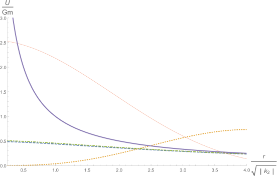
Figure 2: A plot of the modified potential of equations (57) and (60) for a unit mass at the origin ($r=0$). The vertical axis is the scaled potential and the horizontal axis is the distance from the source in terms of the length unit $\sqrt{|k_{2}|}$. The solid curve is the Newtonian potential $1/r$ falloff. The dashed and dotted curves are the solutions in equation (57), with $\chi=-6/25$ and $k_{2}>0$ and $k_{2}<0$, respectively. The dot-dashed and thin curves are the solutions from equation (60) for $\chi=-13/50$, again with $k_{2}>0$ and $k_{2}<0$, respectively.

Returning to the general case of (54), we enumerate the different functional forms of the solution for different regions of the space spanned by the coefficients $k_{1}$, $k_{2}$, $k_{3}$ in Table 1. We assume that we do not make contact with the singular point in $w$ (53), $k_{2}^{2}=k_{1}k_{3}$, as this point would correspond to the dissappearance of the $p^{4}$ term in (45), and would impose a condition on the a priori independent coefficients. Nonetheless we include this case in the appendix 8.5 since it may be of interest. Also, as in section 3.1, we can explore what happens near the apparent singularity in the solution (54), and this is discussed in appendix 8.4.

${\cal G}_{1}$	${\rm sign}(\chi+{\textstyle{{1}\over{4}}})$	$a$, $b$ cond.
${{1}\over{2\pi R}}\Big{[}1+{{1}\over{2}}\left({{\zeta_{1}\zeta_{\alpha}(1+2\chi)}\over{\sqrt{1+4\chi}}}-1\right)e^{\pm iR/\lambda_{+}}$	$+$	$|{\textstyle{{a}\over{b}}}|<1$
$\phantom{spacee}-{{1}\over{2}}\left({{\zeta_{1}\zeta_{\alpha}(1+2\chi)}\over{\sqrt{1+4\chi}}}+1\right)e^{-R/\lambda_{-}}\Big{]}$
${{1}\over{2\pi R}}\Big{[}1+{{1}\over{2}}\left({{\zeta_{1}\zeta_{\alpha}(1+2\chi)}\over{\sqrt{1+4\chi}}}-1\right)e^{\pm iR/\lambda_{+}}$	$+$	${\textstyle{{a}\over{b}}}>1$
$\phantom{spacee}-{{1}\over{2}}\left({{\zeta_{1}\zeta_{\alpha}(1+2\chi)}\over{\sqrt{1+4\chi}}}+1\right)e^{\pm iR/\lambda_{-}}\Big{]}$
${{1}\over{2\pi R}}\Big{[}1+{{1}\over{2}}\left({{\zeta_{1}\zeta_{\alpha}(1+2\chi)}\over{\sqrt{1+4\chi}}}-1\right)e^{-R/\lambda_{+}}$	$+$	${\textstyle{{a}\over{b}}}<-1$
$\phantom{spacee}-{{1}\over{2}}\left({{\zeta_{1}\zeta_{\alpha}(1+2\chi)}\over{\sqrt{1+4\chi}}}+1\right)e^{-R/\lambda_{-}}\Big{]}$
${\textstyle{{1}\over{2\pi R}}}-{\textstyle{{1}\over{2\pi R}}}\exp\left(-{{R}\over{\lambda_{1}}}\right)\Bigg{[}\cos\left({\textstyle{{R}\over{\lambda_{2}}}}\right)-{\textstyle{{\zeta_{1}(1+2\chi)}\over{\sqrt{|1+4\chi|}}}}\sin\left({\textstyle{{R}\over{\lambda_{2}}}}\right)\Bigg{]}$	$-$	N/A

Table 1: Four cases of the general solution (54) for the Newtonian potential Green function ${\cal G}_{1}$, categorized by conditions on the coefficient combinations $k_{1}$, $k_{2}$, and $k_{3}$. Here $a=\zeta_{\alpha}(k_{1}+2k_{2})$ and $b=|k_{1}|\sqrt{1+4\chi}$. The length scales are $\lambda_{\pm}=\sqrt{{{2|k_{2}^{2}-k_{1}k_{3}|}\over{|a\pm b|}}}$ and $\lambda_{1,2}=2\sqrt{{{(k_{2}^{2}-k_{1}k_{3})}\over{(2\sqrt{(k_{2}^{2}-k_{1}k_{3})}-k_{1}-2k_{2})}}}$. For the last row, the case of $\chi+{\textstyle{{1}\over{4}}}<0$ implies $k_{2}^{2}-k_{1}k_{3}>0$.

To end this subsection, we revisit the equations (28) using a perturbative method adopted in past works. This method amounts to assuming the metric components can be obtained from a series $h_{\mu\nu}=h^{(0)}_{\mu\nu}+h^{(1)}_{\mu\nu}+...$. We assume that the $0th$ order, GR solution, satisfies equations (28) for the case of vanishing $k_{1}$, $k_{2}$, and $k_{3}$. Next we solve for the first correction to this solution $h^{(1)}_{\mu\nu}$. Using this method, we find the zeroth and first correction for $h_{00}$ to be given by

$$h_{00}=2U_{0}+\kappa(k_{1}+2k_{2}+k_{3})\rho,$$ (61)

where $U_{0}$ is the usual Newtonian potential from a mass density $\rho$ and the first order correction is a contact term that is nonvanishing only within the mass distribution [16, 91]. The first order solution (61) can be contrasted with the results of Table 1. Clearly the solutions in Table 1 represent a more detailed, careful look at the effects of the isotropic coefficients in (29).

4 Anisotropic exact solutions

While not the main focus of the paper, we discuss features of exact solutions when the coefficients are anisotropic. In the special limit that the only nonzero coefficients in (21) are $k^{(6)0i0j0k0l}$, and still assuming the static matter situation, the equations for $h_{jj}$ and $h_{00}$ can be decoupled. In this case the equation satisfied by $h_{00}$ is given by

$$-\nabla^{2}h_{00}-{\textstyle{{1}\over{2}}}k^{(6)0i0j0k0l}\partial_{ijkl}h_{00}=8\pi G_{N}\rho.$$ (62)

An equation of this form was the subject of Refs. [16] and [17], where a perturbative approach to the solution was taken (with the result contained in (6)). In the perturbative approach, the second term in (62) is treated as much less than the first term, and a zeroth order solution is inserted in for $h_{00}$ in that term. As one of the goals in this paper is to examine the exact, nonperturbative solutions, we attempt here to look at anisotropic cases.

It turns out, exact analytic solutions for (62) for the $15$ independent components of an arbitrary $k^{(6)0i0j0k0l}$ are quite challenging. Instead we examine a special case to show the features of such solutions. We adopt a case where $k^{(6)0i0j0k0l}$ can be written in terms of a contraction $K^{ij}=k^{(6)0i0j0k0k}$ and its trace $K^{jj}$. This reduces (62) to the form,

$$-\nabla^{2}(1+{\textstyle{{3}\over{7}}}K^{ij}\partial_{ij}-{\textstyle{{3}\over{70}}}K^{jj}\nabla^{4})h_{00}=8\pi G_{N}\rho.$$ (63)

Next we assume only diagonal elements $K^{xx}$, $K^{yy}$, and $K^{zz}$, such that $K^{xx}=K^{yy}=K^{zz}/18$, then the equation can be written in the simpler form,

$$\nabla^{2}(1-\lambda^{2}\partial_{z}^{2})h_{00}=-8\pi G_{N}\rho,$$ (64)

where $\lambda=\sqrt{8|K_{zz}|/21}$ and $K_{zz}<0$, so one independent coefficient is left. As before, we construct the Green function solution for a point source. By writing the Green function version of equation (64) as two equations $(1-\lambda^{2}\partial_{z}^{2})\Phi=-\delta^{(3)}(\vec{r})$ and $\nabla^{2}{\cal G}=\Phi$, which can be solved separately [92, 93], and then combining the results, we reduce the answer to an integral over one variable:

$${\cal G}(\rho,z)={{1}\over{8\pi\lambda}}\int^{\infty}_{-\infty}dz^{\prime}{{e^{-|z^{\prime}|/\lambda}}\over{\sqrt{\rho^{2}+(z-z^{\prime})^{2}}}},$$ (65)

where we adopt cylindrical coordinates $\rho,\phi,z$ and $K_{zz}<0$. If instead we consider the case of $K_{zz}>0$, there is a sign change in (65) and the integral changes to

$${\cal G}(\rho,z)={{-i}\over{8\pi\lambda}}\int^{\infty}_{-\infty}dz^{\prime}{{e^{i|z^{\prime}|/\lambda}}\over{\sqrt{\rho^{2}+(z-z^{\prime})^{2}}}}.$$ (66)

We have been unable to evaluate these integrals analytically, so we take a numerical approach.

In the figures 3 and 4, we plot the results from (65) and (66). The standard Newtonian result $1/r$ is plotted along with a numerical evaluation of (65) and (66). In the case of the damped-type solution in (65), we see a narrowed or cuspy behavior of the potential along the $x$ or $y$ direction, and the amplitude is reduced. In the other case of the oscillating-type solution in (66), we see large oscillations along the $z$ direction that do not fall off rapidly.

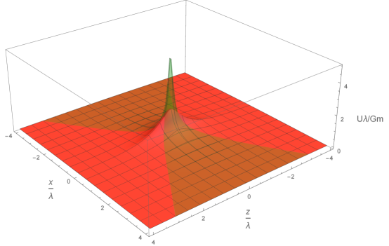
Figure 3: Plot of the scaled anisotropic potential of (65) (damped case), shown in light red versus the Newtonian potential, in transparent green. The source is a point mass at the origin. The behavior is the same in the $y$ direction by the azimuthal symmetry of (65).

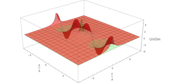
Figure 4: Plot of the scaled anisotropic potential of (66) (oscillating case), shown in light red versus the Newtonian potential, in transparent green. The source is a point mass at the origin. The behavior is the same in the $y$ direction by the aximuthal symmetry of (66).

To contrast with the numerically generated (65) and (66), we outline some features of the perturbative approach. The idea is to solve for the Green function iteratively ${\cal G}={\cal G}_{(0)}+{\cal G}_{(1)}+{\cal G}_{(2)}+...$, where the subscript indicates powers of $\lambda^{2}$. The equations for the $0th$ and subsequent orders are given by

$$\nabla^{2}{\cal G}_{(0)} = -\delta^{(3)}(\vec{r}),$$

$$\nabla^{2}{\cal G}_{(1)} = \lambda^{2}\partial_{z}^{2}\nabla^{2}{\cal G}_{(0)},$$

$$...$$

$$\nabla^{2}{\cal G}_{(n)} = \lambda^{2n}\partial_{z}^{2n}\nabla^{2}{\cal G}_{(n-1)}.$$ (67)

This type of approach is what led to the results in equation (6), where only the first order term is used but arbitrary coefficients assumed.

The $n^{th}$ term in the series (67) can be solved by using standard results for the derivatives of $1/r$ [94]. For ${\cal G}_{(n)}$ we find

$${\cal G}_{(n)}={{\lambda^{2n}}\over{4\pi}}{{(4n-1)!!}\over{r^{2n+1}}}n^{<zzz...>},$$ (68)

where $n^{j}=r^{j}/r$ is a unit vector and $n^{<jkl...>}$ is a symmetric trace free (STF) tensor formed from unit vectors and $\delta^{ij}$ (for example, $n^{<jk>}=n^{j}n^{k}-(1/3)\delta^{ij}$). The STF tensor in (68) is to be evaluated along the $z$ direction. Note that the convergence of such a series is not clear, since, for example, the size of successive terms grow with $n$.

To illustrate this, we plot the exact numerical evaluation of (65) with the successive approximations (67). Figure 5 shows the approximations up to the third term in the series. While the approximations approach the exact answer as $x/\lambda$ decreases, they vary considerably at scales of order $x\sim\lambda$. In fact, it appears successive terms added to the first $G_{(1)}$ are worse than the just the first approximation alone!

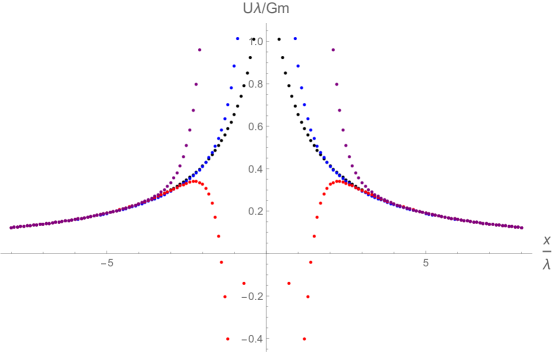
Figure 5: Plot of the potential of (65) along with successive approximations in a perturbative scheme from (67). In black is the exact solution, blue is the first approximation ${\cal G}_{0}+{\cal G}_{1}$, red is the second approximation ${\cal G}_{(0)}+{\cal G}_{(1)}+{\cal G}_{(2)}$, and purple is ${\cal G}_{(0)}+{\cal G}_{(1)}+{\cal G}_{(2)}+{\cal G}_{(3)}$.

From this brief study we can draw several conclusions and open an area for future work. We find that in the case of the damped exponential, where the equation to solve is $(1-\lambda^{2}\partial_{z}^{2})\nabla^{2}{\cal G}_{1}=-\delta^{(3)}(\vec{r})$, the first order approximation follows the exact solution until the $\rho$ and $z$ reach the scale of $\lambda$. This behavior is expected and justifies the use of the perturbative method generally. On the other hand we see from Figure 5, successive terms in a series (67) appear to fail to converge to the exact result. It would be of interest to study in detail how well these approximations could follow an exact solution in general.

Of course, without knowing the true nature of the Newtonian level potential at short ranges from an unknown fundamental theory, we can only speculate. Suppose, hypothetically, that the potential in equations (65) or (66) was indeed the potential coming from an underlying theory of physics. The question then is how well a perturbative approach could match this in the appropriate range. We see above that for some choices of constants, the perturbative approach does not capture the behavior correctly. However, there is an important caveat to include. We truncated the expansion in (3.2) to mass dimension $6$. In the perturbative approach, beyond a first order approximation to the equation $(1+\lambda^{2}\partial_{z}^{2})\nabla^{2}{\cal G}_{1}=-\delta^{(3)}(\vec{r})$, would necessitate the inclusion of mass dimension $8$ terms in the action, for consistency. Indeed, it could be that higher order terms in the action could contribute to an approximation scheme, and provide “counterterms” that result in smooth connection to the underlying potential [95]. For example, imposing requirements term by term in a series expansion, could place theoretical constraints on the coefficients themselves. It would be of interest to attempt a general study of this in gravity or other sectors like the photon sector. Furthermore, this paper studies only the static limit, so it is of interest to study these issues in the time-dependent limit.

Currently, experimental constraints on many of the anisotropic coefficients already exist using experiments that satisfy the experimental constraint of being sensitive enough to measure the Newtonian forces between test masses [96]. Thus if we assume that the perturbative approach is valid, then the coefficient space for anisotropic coefficients is well covered in SR gravity tests [81, 82, 97, 84].

5 Experimental implications

Typical short range gravity tests are designed to measure the attraction between two masses, for instance two flat plates [98, 96]. To see what implications the results of section 3 have on experimental signatures, we plot the gravitational field above a circular disk of mass (figure 6). We include the cases of the Newtonian gravity, the Yukawa potential term (18), and the 4 sample cases of spacetime-symmetry breaking of equations (57) and (60) and display the vertical component in figure 7.

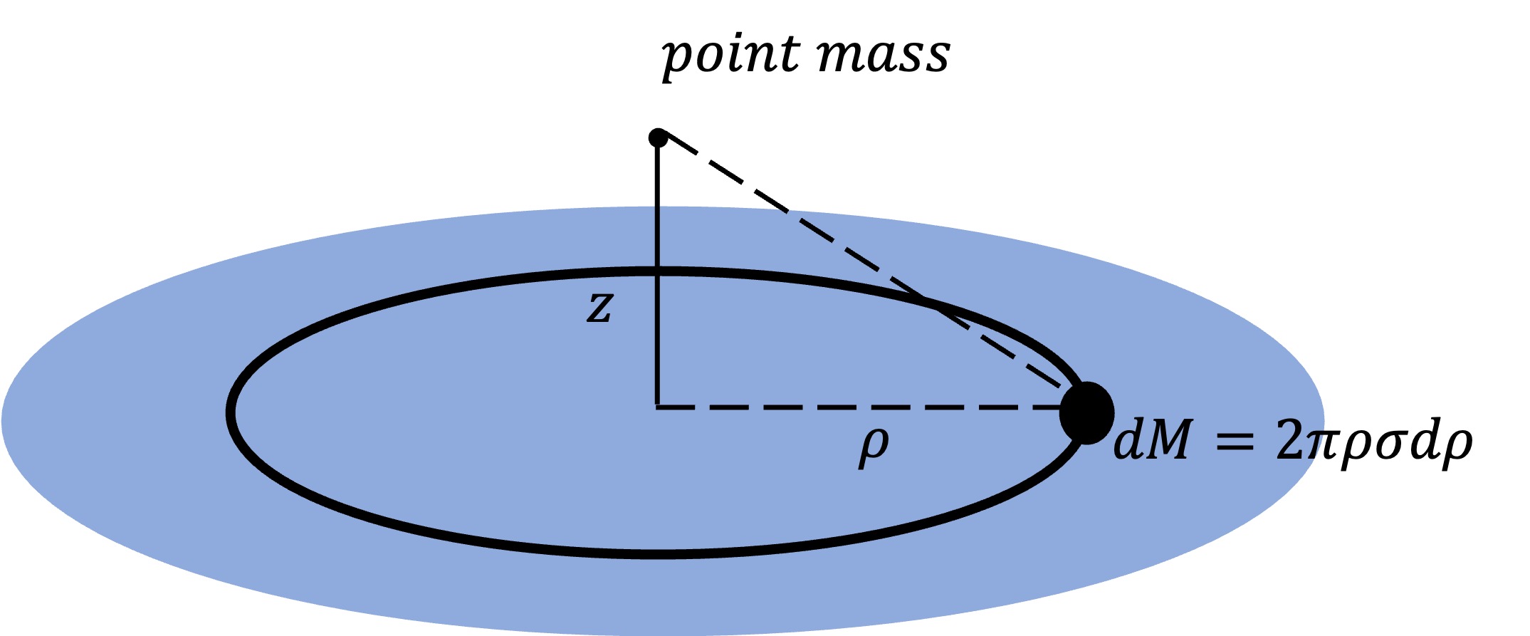
Figure 6: A point mass lies above a thin disk of mass. The gravitational field $\vec{g}=\vec{\nabla}U$ is integrated over this distribution.

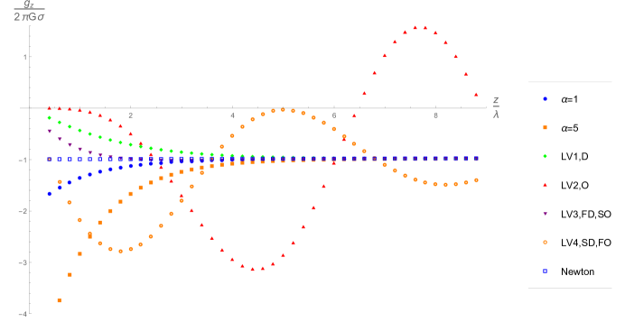
Figure 7: A plot of the gravitational field $g_{z}=\partial U/\partial z$ at a point above the center of a large flat disk of mass. We include two samples of the Yukawa force with $\alpha=1,5$ and the $4$ types of solutions in equations (57) and (60). The vertical axis is the scaled gravitational field and the horizontal axis is the height above the disk $z$ in units relative to the length scale $\lambda$. We set the scale of Lorentz violation to be $\sqrt{|k_{2}|}=\lambda$. The $4$ cases of Lorentz violation show damping only (D), oscillation only (O), and fast damping (FD) with slow oscillation (SO) and finally slow damping (SD) with fast oscillation (FO).

It is clear that the cases studied here exhibit behavior quite different from the Yukawa parametrization. The Yukawa parametrization shows a deviation from the Newtonian case with the force becoming stronger on shorter scales, as expected. The different Lorentz violation cases have oscillatory behavior with and without damping. To get an idea how analysis might proceed, we produce the same plot with one of the $4$ cases, the damped and oscillating solution, but with varying values of $|k_{2}|$, in plot 8. As $|k_{2}|$ becomes smaller, the effects deviating from the Newton case narrow to a region at smaller and smaller length scales. This shows that some of the solutions have the feature that $|k_{2}|$ could be constrained to be below a certain length scale. For example, we can make a crude estimate from Figures 7 and 8: if the Yukawa-type force has been constrained to a region of standard $\alpha-\lambda$ space where $\alpha\sim 1$ and $\lambda\sim 200\mu m$, like the experiment in reference [1], than roughly $\sqrt{k_{2}}<200\mu m$, if one used the specific case of (57).

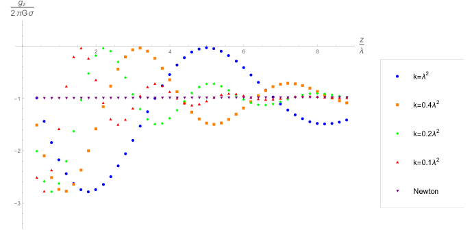
Figure 8: A plot of the gravitational field $g_{z}=\partial U/\partial z$ at a point near a large flat plate of mass. In this plot we let $k_{2}$ vary and show the effect on the damped and oscillating solution from equation (60).

However, what we plot here in Figure 8 is only a one coefficient special case, in the full model one could use each of the cases in Table 1 to fit data and rule out a region of $k_{1}-k_{2}-k_{3}$ space, similar to the way exclusion regions are mapped out in $\alpha-\lambda$ plots in the experimental literature. In general, the region of $k_{1}-k_{2}-k_{3}$ affects the amplitude of the exponential and oscillatory terms and the length scales involved, as can be seen from Table 1.

6 Summary and outlook

In this paper, we studied short-range gravity signals for Lorentz violation that go beyond the leading order approximation, by taking a non-perturbative approach. The focus was on isotropic coefficients, since they are generally harder to measure in experiments and observations. The main results are the coupled field equations for the metric components $h_{00}$ and $h_{jj}$ in the static limit, equations (28), and the general solution for the Green function ${\cal G}_{1}$ for $h_{00}=2U$, organized into four cases in Table 1.

These solutions go beyond the standard Yukawa parametrization (18) and could be studied in short-range gravity tests of all kinds. Particularly, it may be of interest for short-range tests that probe large non-Newtonian forces. One option for data analysis is to restrict attention to the solutions in the last two rows in Table 1, which do not exhibit undamped oscillations. One could then attempt to use experimental data to measure the coefficient combinations $k_{1}$, $k_{2}$, and $k_{3}$ (equation (29)) contained in these expressions. Analysis could also proceed with a simpler two coefficient special case model in section 3.1, or, in the case of tests sensitive to very large non-Newtonian forces, one could use the large amplitude, $\chi=-1/4+\epsilon$ limit, outlined in the appendix and Table 4.

The isotropic mass dimension $6$ coefficients that can be probed using the solutions in this work, in equations (29), appear to be distinct combinations from the combination appearing in gravitational wave propagation tests [99], as shown in (83). This demonstrates the usefulness of additional short-range gravity test analysis outlined in this work, providing an independent probe of isotropic coefficients from GW tests.

In this work, we also collect some useful pedagogical results with explicit examples of the construction of isotropic coefficients from Young Tableau, as discussed in appendix 8.3. In section 4 we discussed exact solutions in the case of anisotropic coefficients, and compared the results to perturbative methods used so far. It would be of interest to compute integrals like (65) and (66) analytically, if possible. In addition, a study of the convergence of the series (67) and related topics like adding time dependence would be of interest. Considerations of this paper could be applied to the photon sector [77, 100], where, analogous to gravity, new types of massive photon-like signals may be revealed.

7 Acknowledgements

The authors acknowledge support from the National Science Foundation under grants 1806871 and 2207734. We thank Embry-Riddle Aeronautical University’s Undergraduate Research Institute for support of Jennifer L. James and Janessa R. Slone. Valuable comments on the manuscript have been provided by Brett Altschul, V. Alan Kostelecký, and Rui Xu.

8 Appendix

8.1 Special Case Model

We record the exact field equations for the action in (7), ${\cal L}={\textstyle{{1}\over{2\kappa}}}\sqrt{-g}\left(R+k_{\alpha\beta}R^{\alpha\beta}R\right)$. Upon variation with respect to the full metric $g_{\mu\nu}$ we obtain:

$$G^{\mu\nu} = {\textstyle{{1}\over{2}}}g^{\mu\nu}k_{\alpha\beta}R^{\alpha\beta}R-k_{\alpha}^{\phantom{\alpha}\mu}R^{\nu\alpha}R-k_{\alpha}^{\phantom{\alpha}\nu}R^{\mu\alpha}R-k_{\alpha\beta}R^{\alpha\beta}R^{\mu\nu}$$ (69)

$$-{\textstyle{{1}\over{2}}}g^{\mu\nu}\nabla^{\alpha}\nabla^{\beta}(k_{\alpha\beta}R)-g^{\mu\nu}\nabla^{2}(k_{\alpha\beta}R^{\alpha\beta})$$

$$+{\textstyle{{1}\over{2}}}\nabla_{\alpha}\nabla^{\mu}(k^{\nu\alpha}R)+{\textstyle{{1}\over{2}}}\nabla_{\alpha}\nabla^{\nu}(k^{\mu\alpha}R)$$

$$+\nabla^{\mu}\nabla^{\nu}(k_{\alpha\beta}R^{\alpha\beta})-{\textstyle{{1}\over{2}}}\nabla^{\alpha}\nabla_{\alpha}(k^{\mu\nu}R).$$

Here we treat $k_{\alpha\beta}$ as a fixed background set of coefficients and do not consider field equations obtained with the variation $\delta k_{\alpha\beta}$, but this could be generalized.

8.2 Differential equation results

Here we record some basic results that we use in constructing the general solutions for the PDE’s in the paper. Boundary conditions are assumed where the fields vanish at spatial infinity. First we note the Helmholtz equation for a field $\psi$

$$(\nabla^{2}+\omega^{2})\psi=-\delta^{(3)}(\vec{R}).$$ (70)

This is solved with the following Green function (e.g., see Ref. [92])

$$\psi={{e^{\pm i\omega R}}\over{4\pi R}}.$$ (71)

Note that if $\omega$ is a general complex number, $\omega=a+ib$ then one obtains

$$\psi={{e^{\pm iaR}}\over{4\pi R}}e^{\mp bR},$$ (72)

which shows that oscillation and damping or growth can occur. When $a=0$ and $\mp b<0$, then the solution to the Proca or modified Helmholtz equation is recovered.

We also record here the less common nonlocal equation considered long ago in generalized electrodynamics [37, 38],

$$(\nabla^{2}-\lambda^{2}\nabla^{4})\psi=-\delta^{(3)}(\vec{R}).$$ (73)

For this equation, the Green function is (e.g., see Ref. [93]),

$$\psi={{1}\over{4\pi R}}-{{e^{-R/\lambda}}\over{4\pi R}}.$$ (74)

Here again, $\lambda$ could be complex, yielding oscillatory behavior.

8.3 Isotropic limit of coefficients

We record here the portion of the field equations in the static limit involving the $\delta M^{\mu\nu\rho\sigma}h_{\rho\sigma}$ (definition in Eq. (21)). It is useful in what follows to enumerate the specific tensor symmetries of the coefficients involved (5). For convenience, we display here the young tableau [45] for the coefficients with spacetime indices:

$$s^{(4)\mu\rho\epsilon\nu\sigma\zeta} \Leftrightarrow \young(\mu\nu,\rho\sigma,\epsilon\zeta),$$

$$q^{(5)\mu\nu\kappa\alpha\beta\gamma\delta} \Leftrightarrow \young(\mu\alpha\gamma,\nu\beta\delta,\kappa),$$

$$s^{(6)\mu\rho\epsilon\nu\sigma\zeta\alpha\beta} \Leftrightarrow \young(\mu\nu\alpha\beta,\rho\sigma,\epsilon\zeta),$$

$$k^{(6)\mu\epsilon\nu\zeta\rho\alpha\sigma\beta} \Leftrightarrow \young(\mu\nu\rho\sigma,\epsilon\zeta\alpha\beta).$$ (75)

Later below, we break down these coefficients into spatial subsets. Young tableau and the process of breaking down Tableau into representations of subgroups is described elsewhere [101, 102].

For the space and time components $\delta M^{00\rho\sigma}h_{\rho\sigma}$, $\delta M^{0i\rho\sigma}h_{\rho\sigma}$, and $\delta M^{ij\rho\sigma}h_{\rho\sigma}$, we obtain

$$\delta M^{00\rho\sigma}h_{\rho\sigma} = -{\textstyle{{1}\over{2}}}k^{(6)0i0j0k0l}\partial_{ijkl}h_{00}$$ (76)

$$-\{{\textstyle{{1}\over{2}}}k^{(6)0j0k0lim}\partial_{jklm}+{\textstyle{{1}\over{4}}}q^{(5)0ij0k0l}\partial_{jkl}\}h_{0i}$$

$$-\{{\textstyle{{1}\over{2}}}[s^{(4)0ik0jl}\partial_{kl}+s^{(6)0ik0jlmn}\partial_{klmn}+k^{(6)0k0limjn}\partial_{klmn}]$$

$$\phantom{--}+{\textstyle{{1}\over{4}}}[q^{(5)0ik0ljm}+q^{(5)0jk0lim}]\partial_{klm}\}h_{ij},$$

$$\delta M^{0i\rho\sigma}h_{\rho\sigma} = -\{{\textstyle{{1}\over{2}}}k^{(6)0kil0m0n}\partial_{klmn}-{\textstyle{{1}\over{4}}}q^{(5)0ik0l0m}\partial_{klm}\}h_{00}$$ (77)

$$+\{{\textstyle{{1}\over{4}}}[s^{(4)0ik0jl}\partial_{kl}+s^{(6)0ik0jlmn}\partial_{klmn}]-{\textstyle{{1}\over{2}}}k^{(6)0kilomjn}\partial_{klmn}$$

$$-{\textstyle{{1}\over{8}}}[-q^{(5)0ik0ljm}+q^{(5)0jk0lim}+q^{(5)ijk0l0m}]\partial_{klm}\}h_{0j}$$

$$-\{{\textstyle{{1}\over{2}}}[s^{(4)0jlikm}\partial_{lm}+s^{(6)0jlikmnp}\partial_{lmnp}]+{\textstyle{{1}\over{2}}}k^{(6)0limjnkp}\partial_{lmnp}$$

$$+{\textstyle{{1}\over{4}}}[q^{(5)0jlimkn}+q^{(5)ijl0mkn}]\partial_{lmn}\}h_{jk},$$

$$\delta M^{ij\rho\sigma}h_{\rho\sigma} = -\{{\textstyle{{1}\over{2}}}[s^{(4)0ik0jl}\partial_{kl}+s^{(6)0ik0jlmn}\partial_{klmn}]$$ (78)

$$+{\textstyle{{1}\over{2}}}k^{(6)ikjl0m0n}\partial_{klmn}+{\textstyle{{1}\over{4}}}[q^{(5)0ik0ljm}+q^{(5)0jk0lim}]\partial_{klm}\}h_{00}$$

$$-\{{\textstyle{{1}\over{4}}}[s^{(4)i0ljkm}\partial_{lm}+s^{(6)i0ljkmnp}\partial_{lmnp}]+{\textstyle{{1}\over{4}}}[i\rightleftharpoons j]$$

$$\phantom{++}+{\textstyle{{1}\over{2}}}k^{(6)0lkminjp}\partial_{lmnp}+{\textstyle{{1}\over{8}}}[q^{(5)i0ljmkn}+q^{(5)j0limkn}$$

$$\phantom{++}+q^{(5)ikljm0n}+q^{(5)jklim0n}]\partial_{lmn}\}h_{0k}$$

$$-\{{\textstyle{{1}\over{2}}}[s^{(4)ikmjln}\partial_{mn}+s^{(6)ikmjlnpq}\partial_{mnpq}]+{\textstyle{{1}\over{2}}}k^{(6)imjnkplq}\partial_{mnpq}$$

$$+{\textstyle{{1}\over{4}}}[q^{(5)ikmjnlp}+q^{(5)jkminlp}]\partial_{mnp}\}h_{kl},$$

where we have already used the tensor symmetry properties of the coefficients in (5). To simplify the terms occuring in (78), we assume only isotropic coefficients and express each set of coefficients occurring in (78) in terms of its scalar contractions. To elucidate the process, the results for each of the coefficients are recorded in Tables 2 and 3 below. Note that isotropic limits of the coefficients are of interest independently of the present paper. This is due to the challenges of their measurement with the same precision as anisotropic coefficients [103].

Coefficients	Tableau	isotropic form
$s^{(4)0ik0jl}$	$\young(ij,kl)$	${\textstyle{{1}\over{6}}}(\delta^{ij}\delta^{kl}-\delta^{kj}\delta^{il})s^{(4)0mn0mn}$
$s^{(4)0jlikm}$	$\young(ij,kl,m)$	$0$
$s^{(4)ikmjln}$	$\young(ij,kl,mn)$	${\textstyle{{1}\over{6}}}\epsilon^{ikm}\epsilon^{jln}s^{(4)pqrpqr}$
$q^{(5)0ij0k0l}$	$\young(ikl,j)$	$0$
$q^{(5)0ik0ljm}$	$\young(ijl,km)$	$0$
$q^{(5)ijk0l0m}$	$\young(ilm,j,k)$	$-{{1}\over{3}}\epsilon^{ijk}\delta^{lm}(^{*}q_{0}^{\phantom{0}0n0n})$
$q^{(5)0jlimkn}$	$\young(jik,lmn)$	$0$
$q^{(5)ijl0mkn}$	$\young(ikm,jn,l)$	$0$
$q^{(5)ikmjnlp}$	$\young(ijl,knp,m)$	$-{{1}\over{6}}\epsilon^{ikm}(\delta^{jl}\delta^{np}-\delta^{jp}\delta^{nl})(^{*}q_{0}^{\phantom{0}qrqr})$

Table 2: Mass dimension 4 and 5 coefficients expressed assuming isotropic coefficients only. The dual is defined by ${}^{*}q_{\lambda}^{\phantom{\lambda}\alpha\beta\gamma\delta}=-{\textstyle{{1}\over{3!}}}\epsilon_{\lambda\mu\nu\kappa}q^{\mu\nu\kappa\alpha\beta\gamma\delta}$ with $\epsilon_{0123}=+1$.

Coefficients	Tableau	isotropic form
$s^{(6)0ik0jlmn}$	$\young(ijmn,kl)$	${\textstyle{{1}\over{60}}}(\delta^{in}\delta^{jm}\delta^{kl}+\delta^{im}\delta^{jn}\delta^{kl}-\delta^{il}\delta^{jn}\delta^{km}-\delta^{il}\delta^{jm}\delta^{kn}$
		$-\delta^{in}\delta^{jk}\delta^{lm}+\delta^{ij}\delta^{kn}\delta^{lm}-\delta^{im}\delta^{jk}\delta^{ln}+\delta^{ij}\delta^{km}\delta^{ln}$
		$-2\delta^{il}\delta^{jk}\delta^{mn}+2\delta^{ij}\delta^{kl}\delta^{mn})s^{(6)0pq0pqrr}$
$s^{(6)0jlikmnp}$	$\young(ijnp,kl,m)$	$0$
$s^{(6)ikmjlnpq}$	$\young(ijpq,kl,mn)$	${\textstyle{{1}\over{90}}}(-\delta^{iq}\delta^{jp}\delta^{kn}\delta^{lm}-\delta^{ip}\delta^{jq}\delta^{kn}\delta^{lm}$
		$+\delta^{in}\delta^{jq}\delta^{kp}\delta^{lm}+...)s^{(6)rstrstuu}$
$k^{(6)0i0j0k0l}$	$\young(ijkl)$	${\textstyle{{1}\over{15}}}(\delta^{ij}\delta^{kl}+\delta^{ik}\delta^{jl}+\delta^{il}\delta^{jk})k^{(6)0m0m0n0n}$
$k^{(6)0j0k0lim}$	$\young(iljk,m)$	0
$k^{(6)0k0limjn}$	$\young(ijkl,mn)$	${\textstyle{{1}\over{60}}}(-2\delta^{in}\delta^{jm}\delta^{kl}-\delta^{in}\delta^{jl}\delta^{km}-\delta^{il}\delta^{jm}\delta^{kn}-\delta^{in}\delta^{jk}\delta^{lm}$
		$+\delta^{ij}\delta^{kn}\delta^{lm}-\delta^{ik}\delta^{jm}\delta^{ln}+\delta^{ij}\delta^{km}\delta^{ln}+\delta^{il}\delta^{jk}\delta^{mn}$
		$+\delta^{ik}\delta^{jl}\delta^{mn}+2\delta^{ij}\delta^{kl}\delta^{mn})k^{(6)0p0pqrqr}$
$k^{(6)0kil0mjn}$		$k^{(6)0kil0mjn}=k^{(6)0k0limjn}-k^{(6)0k0ilmjn}$
$k^{(6)0limjnkp}$	(jkil,npm)	$0$
$k^{(6)imjnkplq}$	(ijkl,mnpq)	${\textstyle{{1}\over{240}}}(2\delta^{iq}\delta^{jp}\delta^{kn}\delta^{lm}+\delta^{ip}\delta^{jq}\delta^{kn}\delta^{lm}$
		$+\delta^{in}\delta^{jp}\delta^{kq}\delta^{lm}+...)k^{(6)rsrstutu}$

Table 3: Mass dimension 6 coefficients expressed assuming isotropic coefficients only. For two of the sets of coefficients, $s^{(6)ikmjlnpq}$ and $k^{(6)imjnkplq}$, the expression in terms of Kronecker deltas is abbreviated due to its length. It can be calculated using the “YoungProject” command of the xTras package for xTensor [104].

The results from the Tables 2 and 3 are then inserted in the expressions (78) and simplified to the following:

$$\delta M^{00\rho\sigma}h_{\rho\sigma} = -{\textstyle{{1}\over{10}}}k^{(6)0m0m0n0n}\nabla^{4}h_{00}$$ (79)

$$+\{{\textstyle{{1}\over{12}}}s^{(4)0kl0kl}+{\textstyle{{1}\over{30}}}s^{(6)0kl0klmm}\nabla^{2}+{\textstyle{{1}\over{30}}}k^{(6)0k0klmlm}\nabla^{2}\}$$

$$\times(\partial_{i}\partial_{j}-\delta_{ij}\nabla^{2})h_{ij},$$

$$\delta M^{0i\rho\sigma}h_{\rho\sigma} = \{{\textstyle{{1}\over{24}}}s^{(4)0kl0kl}+{\textstyle{{1}\over{60}}}s^{(6)0kl0klmm}\nabla^{2}-{\textstyle{{1}\over{30}}}k^{(6)0k0klmlm}\nabla^{2}\}$$ (80)

$$\times(\delta_{ij}\nabla^{2}-\partial_{i}\partial_{j})h_{0j}$$

$$-{\textstyle{{1}\over{24}}}(^{*}q_{0}^{\phantom{0}0l0l})\epsilon_{ijk}\nabla^{2}\partial_{j}h_{0k},$$

$$\delta M^{ij\rho\sigma}h_{\rho\sigma} = \{-{\textstyle{{1}\over{12}}}(s^{(4)0kl0kl}+{\textstyle{{1}\over{2}}}s^{(4)klmklm})$$ (81)

$$\phantom{s}-{\textstyle{{1}\over{30}}}(s^{(6)0kl0klmm}+k^{(6)0k0klmlm})\nabla^{2}$$

$$\phantom{s}-{\textstyle{{1}\over{72}}}s^{(6)klmklmnn}\nabla^{2}-{\textstyle{{1}\over{240}}}k^{(6)klklmnmn}\nabla^{2}\}\delta^{ij}\nabla^{2}h_{00}$$

$$+\{{\textstyle{{1}\over{12}}}(s^{(4)0kl0kl}+s^{(4)klmklm})$$

$$\phantom{s}+{\textstyle{{1}\over{30}}}(s^{(6)0kl0klmm}+k^{(6)0k0klmlm})\nabla^{2}$$

$$\phantom{sm}+{\textstyle{{1}\over{36}}}s^{(6)klmklmnn}\nabla^{2}-{\textstyle{{1}\over{240}}}k^{(6)klklmnmn}\nabla^{2}\}\partial_{ij}h_{00}$$

$$-\{{\textstyle{{1}\over{24}}}s^{(4)klmklm}+{\textstyle{{1}\over{72}}}s^{(6)klmklmnn}\nabla^{2}$$

$$\phantom{sm}+{\textstyle{{1}\over{240}}}k^{(6)klklmnmn}\nabla^{2}\}\delta^{ij}\nabla^{2}h_{pp}$$

$$+\{{\textstyle{{1}\over{12}}}s^{(4)klmklm})+{\textstyle{{1}\over{36}}}s^{(6)klmklmnn}\nabla^{2}$$

$$\phantom{sm}-{\textstyle{{1}\over{60}}}k^{(6)klklmnmn}\nabla^{2}\}\nabla^{2}h_{ij}$$

$$+{\textstyle{{1}\over{80}}}k^{(6)klklmnmn}\nabla^{2}\partial_{ij}h_{pp}$$

$$-{\textstyle{{1}\over{24}}}^{*}q_{0}^{\phantom{0}lnln}(\epsilon_{mki}\partial_{m}\nabla^{2}h_{jk}+\epsilon_{mkj}\partial_{m}\nabla^{2}h_{ik}).$$

Note that for the last of equations (81), one takes the trace in $ij$ to obtain the result (28). The equations for the off-diagonal components $h_{ij}-{\textstyle{{1}\over{3}}}\delta_{ij}h_{kk}$ can be obtained from (81) by subtracting the trace appropriately. Like the sample case in Section 3.1 (see equation (11)) $h_{ij}-{\textstyle{{1}\over{3}}}\delta_{ij}h_{kk}$ is sourced by $h_{00}$ and $h_{jj}$ and since $h_{00}$ is of primary interest in this work we do not include the solution here.

To compare the results with those obtained by looking at propagation effects in gravitational waves, we record here the isotropic combination of coefficients in the gravity sector called $(k_{I}^{(6)})_{00}$. The spherical coefficients are defined by (see reference [99]),

$${\textstyle{{1}\over{2}}}({\hat{s}}^{+-+-}+{\hat{k}}^{++--})=\sum_{jm}\omega^{4}(-1)^{j}Y_{jm}(\hat{v})(k_{I}^{(6)})_{jm},$$ (82)

where the coefficients on the left hand side are to be evaluated at $d=6$ only, and from (5) with the substitution $\partial_{\mu}\rightarrow-ip_{\mu}$. The $+$, $-$, and the $\hat{v}$ refer to a helicity basis for GW’s so that $p_{\mu}=(-1,\hat{v})$. A plus or minus in an index indicates a contraction with the helicity basis vectors ${\bf e}^{+}$ and ${\bf e}^{-}$ (see Ref. [99, 77] for more details). Focusing on only the isotropic piece $(k_{I}^{(6)})_{00}$ it can be shown the following relation holds:

$$(k_{I}^{(6)})_{00} = \sqrt{4\pi}\Big{[}-{\textstyle{{1}\over{12}}}(s^{(6)0ij0ij00}+s^{(6)ijkijk00}+{\textstyle{{1}\over{5}}}s^{(6)0ij0ijkk}+{\textstyle{{1}\over{3}}}s^{(6)ijkijkll})$$ (83)

$$\phantom{space}+{\textstyle{{1}\over{60}}}(4k^{(6)0i0i0j0j}+8k^{(6)0i0ijkjk}+k^{(6)ijijklkl})\Big{]}.$$

8.4 Large amplitude limit of the solution

Given the results of the section 3.2, we record here the large amplitude limit, where $\chi\sim-1/4$. Specifically we let $\chi=-1/4+\epsilon$ and explore the solutions for small $\epsilon$. When simplifying the solution (54) in this limit, the result depends on the sign of the coefficient combination $k_{2}+2k_{3}$ and the sign of $\epsilon$. Thus the result breaks into 4 cases. Specifically, when expanding to the lowest order in $\epsilon$ we find the four solutions in the Table 4.

${\cal G}_{1}$	${\rm sgn}(k_{2}+2k_{3})$	${\rm sgn}\epsilon$
${\textstyle{{1}\over{2\pi R}}}\Bigg{[}1-{{1}\over{2}}\exp\left(-{\textstyle{{R}\over{\sqrt{|k_{2}+2k_{3}|}}}}\right)\Big{[}2+\psi{\textstyle{{R}\over{\sqrt{|k_{2}+2k_{3}|}}}}\Big{]}$	$+$	$+$
${\textstyle{{1}\over{2\pi R}}}\Bigg{[}1-{{1}\over{2}}\exp\left({\textstyle{{\pm iR}\over{\sqrt{|k_{2}+2k_{3}|}}}}\right)\Big{[}2\pm i\psi{\textstyle{{R}\over{\sqrt{|k_{2}+2k_{3}|}}}}\Big{]}$	$-$	$+$
${\textstyle{{1}\over{2\pi R}}}-{\textstyle{{1}\over{2\pi R}}}\exp\left(-{{R}\over{\sqrt{|k_{2}+2k_{3}|}}}\right)\Bigg{[}\cos\left(2\psi\sqrt{{{|\epsilon|}\over{|k_{2}+2k_{3}|}}}R\right)$	$+$	$-$
$\phantom{spacespace}+{\textstyle{{1}\over{4\sqrt{|\epsilon|}}}}\sin\left(2\psi\sqrt{{{|\epsilon|}\over{|k_{2}+2k_{3}|}}}R\right)\Bigg{]}$
${\textstyle{{1}\over{2\pi R}}}-{\textstyle{{1}\over{2\pi R}}}\exp\left(-2\psi\sqrt{{{|\epsilon|}\over{|k_{2}+2k_{3}|}}}R\right)\Bigg{[}\cos\left({{R}\over{\sqrt{|k_{2}+2k_{3}|}}}\right)$	$-$	$-$
$\phantom{spacespace}+{\textstyle{{1}\over{4\sqrt{|\epsilon|}}}}\sin\left({{R}\over{\sqrt{|k_{2}+2k_{3}|}}}\right)\Bigg{]}$

Table 4: Solutions for the Green function ${\cal G}_{1}$ from equation (54) in the (large amplitude) limit where $\chi=-1/4+\epsilon$ for small $\epsilon$. The sign choice for $\epsilon$ and the coefficient combination $k_{2}+2k_{3}$ are listed in the right two columns. Here, $\psi=|k_{2}+k_{3}|/|k_{2}+2k_{3}|$ and the coefficient combinations $k_{1}$, $k_{2}$, and $k_{3}$ are defined in equation (29). Note that $\psi$ and $R/|k_{2}+2k_{3}|$ must be of $O(1)$ or smaller for the approximation to be valid. Error terms for these approximations are of order $\sqrt{\epsilon}$.

Several features are clear in this limit. Firstly, as $\epsilon\rightarrow 0$, it can be shown that 3 of the 4 solutions in Table 4 are finite. The fourth row, with ${\rm sgn}(k_{2}+2k_{3})=-1$ and ${\rm sgn}\epsilon=-1$ diverges as $\epsilon\rightarrow 0$. Second, the solutions are oscillatory in $R$ with no damping (second row $-+$ case), a mixture of damped and oscillatory behavior in $R$ (third and fourth row $+-$ and $--$ cases), or damped with no oscillations (first row $++$ case). The nature of the solution depends critically on which part of the $k_{1}$, $k_{2}$, $k_{3}$ coefficient space one probes.

8.5 Special cases: $k_{2}^{2}-k_{1}k_{3}=0\vee k_{1}+2k_{2}=0$

We record here the solution for the Green function for the Newtonian potential when the coefficient combinations $k_{1}$, $k_{2}$, and $k_{3}$ ((29)) take on special values. When $k_{2}^{2}-k_{1}k_{3}=0$, we cannot apply the solution (54) directly. We go back to re-evaluate the Fourier transform integral (47) with the $p^{4}$ term absent. The result for $G_{1}$, and $G_{2}$, the Green functions for ${\bar{h}}_{00}$ and ${\bar{h}}_{jj}$, are given by

$$G_{1}(\vec{r},\vec{r}^{\prime}) = {{1}\over{\pi R}}\left(1-{{k_{1}+k_{2}}\over{k_{1}+2k_{2}}}e^{-i{\textstyle{{R}\over{\sqrt{k_{1}+2k_{2}}}}}}\right),$$

$$G_{2}(\vec{r},\vec{r}^{\prime}) = -{{1}\over{\pi R}}{{k_{2}+k_{3}}\over{k_{1}+2k_{2}}}e^{-i{\textstyle{{R}\over{\sqrt{k_{1}+2k_{2}}}}}}.$$ (84)

Note that when the sign of $k_{1}+2k_{2}$ is negative, the solution becomes a damped exponential of the Yukawa form. The Green function for $h_{00}$ can be obtained from ${\cal G}_{1}=(1/2)(G_{1}+G_{2})$.

Also we consider here the special case when $k_{2}^{2}-k_{1}k_{3}=0$ and $k_{1}+2k_{2}=0$. In this case the nonstandard terms in the momentum space functions in (46) are constants, yielding delta functions with the Fourier transform. The Green function ${\cal G}_{1}$ is then given by

$${\cal G}_{1}={{1}\over{2\pi R}}+2k_{3}\delta^{(3)}(\vec{R}).$$ (85)

9 References

References

- [1] J. G. Lee, E. G. Adelberger, T. S. Cook, S. M. Fleischer, and B. R. Heckel. New test of the gravitational law at separations down to . Phys. Rev. Lett., 124:101101, Mar 2020.
- [2] Yasunori Fujii. Dilaton and possible non-newtonian gravity. Nature, 234:5–7, 1971.
- [3] John F Donoghue. Introduction to the effective field theory description of gravity. Advanced school on effective theories: Almunecar, Granada, Spain, 26:217–240, 1995.
- [4] Nima Arkani-Hamed, Savas Dimopoulos, and G. R. Dvali. The Hierarchy problem and new dimensions at a millimeter. Phys. Lett. B, 429:263–272, 1998.
- [5] Ephraim Fischbach and Carrick L Talmadge. The search for non-Newtonian gravity. Springer Science & Business Media, 1998.
- [6] Dennis E. Krause and Ephraim Fischbach. Searching for extra dimensions and new string inspired forces in the Casimir regime. Lect. Notes Phys., 562:292–309, 2001.
- [7] Jiro Murata and Saki Tanaka. A review of short-range gravity experiments in the LHC era. Class. Quant. Grav., 32(3):033001, 2015.
- [8] E. G. Adelberger, Blayne R. Heckel, and A. E. Nelson. Tests of the gravitational inverse square law. Ann. Rev. Nucl. Part. Sci., 53:77–121, 2003.
- [9] V. Alan Kostelecký and Stuart Samuel. Spontaneous breaking of lorentz symmetry in string theory. Phys. Rev. D, 39:683–685, Jan 1989.
- [10] Rodolfo Gambini and Jorge Pullin. Nonstandard optics from quantum space-time. Phys. Rev. D, 59:124021, May 1999.
- [11] Sean M. Carroll, Jeffrey A. Harvey, V. Alan Kostelecký, Charles D. Lane, and Takemi Okamoto. Noncommutative field theory and lorentz violation. Phys. Rev. Lett., 87:141601, Sep 2001.
- [12] David Mattingly. Modern tests of Lorentz invariance. Living Rev. Rel., 8:5, 2005.
- [13] Jay D. Tasson. What Do We Know About Lorentz Invariance? Rept. Prog. Phys., 77:062901, 2014.
- [14] A. Addazi et al. Quantum gravity phenomenology at the dawn of the multi-messenger era—A review. Prog. Part. Nucl. Phys., 125:103948, 2022.
- [15] T Mariz, JR Nascimento, and A Yu Petrov. Lorentz symmetry breaking–classical and quantum aspects. arXiv preprint arXiv:2205.02594, 2022.
- [16] Quentin G. Bailey, Alan Kostelecký, and Rui Xu. Short-range gravity and Lorentz violation. Phys. Rev. D, 91(2):022006, 2015.
- [17] V. Alan Kostelecký and Matthew Mewes. Testing local Lorentz invariance with short-range gravity. Phys. Lett. B, 766:137–143, 2017.
- [18] Steven Weinberg. Effective Field Theory, Past and Future. PoS, CD09:001, 2009.
- [19] V. Alan Kostelecky and Robertus Potting. CPT, strings, and meson factories. Phys. Rev. D, 51:3923–3935, 1995.
- [20] Don Colladay and V. Alan Kostelecký. violation and the standard model. Phys. Rev. D, 55:6760–6774, Jun 1997.
- [21] D. Colladay and V. Alan Kostelecký. Lorentz-violating extension of the standard model. Phys. Rev. D, 58:116002, Oct 1998.
- [22] V. Alan Kostelecký. Gravity, lorentz violation, and the standard model. Phys. Rev. D, 69:105009, May 2004.
- [23] Neil Cornish, Laura Sampson, Nicolas Yunes, and Frans Pretorius. Gravitational Wave Tests of General Relativity with the Parameterized Post-Einsteinian Framework. Phys. Rev. D, 84:062003, 2011.
- [24] Saeed Mirshekari, Nicolás Yunes, and Clifford M. Will. Constraining lorentz-violating, modified dispersion relations with gravitational waves. Phys. Rev. D, 85:024041, Jan 2012.
- [25] Clifford M. Will. The Confrontation between General Relativity and Experiment. Living Rev. Rel., 17:4, 2014.
- [26] Ted Jacobson and David Mattingly. Gravity with a dynamical preferred frame. Phys. Rev. D, 64:024028, 2001.
- [27] Stephon Alexander and Nicolas Yunes. Chern-Simons Modified General Relativity. Phys. Rept., 480:1–55, 2009.
- [28] Emanuele Berti et al. Testing General Relativity with Present and Future Astrophysical Observations. Class. Quant. Grav., 32:243001, 2015.
- [29] Maria Okounkova, Will M. Farr, Maximiliano Isi, and Leo C. Stein. Constraining gravitational wave amplitude birefringence and Chern-Simons gravity with GWTC-2. Phys. Rev. D, 106(4):044067, 2022.
- [30] F. W. Hehl, P. Von Der Heyde, G. D. Kerlick, and J. M. Nester. General Relativity with Spin and Torsion: Foundations and Prospects. Rev. Mod. Phys., 48:393–416, 1976.
- [31] Robert Bluhm. Explicit versus spontaneous diffeomorphism breaking in gravity. Phys. Rev. D, 91:065034, Mar 2015.
- [32] V. Alan Kostelecký and Zonghao Li. Backgrounds in gravitational effective field theory. Phys. Rev. D, 103:024059, Jan 2021.
- [33] Ephraim Fischbach, Mark P. Haugan, Dubravko Tadic, and Hai-Yang Cheng. Lorentz Noninvariance and the Eotvos Experiments. Phys. Rev. D, 32:154, 1985.
- [34] V. Alan Kostelecky and Jay Tasson. Prospects for Large Relativity Violations in Matter-Gravity Couplings. Phys. Rev. Lett., 102:010402, 2009.
- [35] Alan V. Kostelecky and Jay D. Tasson. Matter-gravity couplings and Lorentz violation. Phys. Rev. D, 83:016013, 2011.
- [36] Hélène Pihan-Le Bars et al. New Test of Lorentz Invariance Using the MICROSCOPE Space Mission. Phys. Rev. Lett., 123(23):231102, 2019.
- [37] Boris Podolsky. A Generalized Electrodynamics Part I-Non-Quantum. Phys. Rev., 62:68–71, 1942.
- [38] A. Pais and G. E. Uhlenbeck. On Field theories with nonlocalized action. Phys. Rev., 79:145–165, 1950.
- [39] Richard P. Woodard. Ostrogradsky’s theorem on Hamiltonian instability. Scholarpedia, 10(8):32243, 2015.
- [40] Quentin G. Bailey. Construction of higher-order metric fluctuation terms in spacetime symmetry-breaking effective field theory. Symmetry, 13(5), 2021.
- [41] Yuri Bonder and Christian Peterson. Explicit Lorentz violation in a static and spherically-symmetric spacetime. Phys. Rev. D, 101(6):064056, 2020.
- [42] Kellie O’Neal-Ault, Quentin G. Bailey, and Nils A. Nilsson. 3+1 formulation of the standard-model extension gravity sector. Physical Review D, 103(4), feb 2021.
- [43] Carlos M. Reyes and Marco Schreck. Hamiltonian formulation of an effective modified gravity with nondynamical background fields. Phys. Rev. D, 104(12):124042, 2021.
- [44] Carlos M. Reyes and Marco Schreck. Modified-gravity theories with nondynamical background fields. Phys. Rev. D, 106(4):044050, 2022.
- [45] V. Alan Kostelecký and Matthew Mewes. Testing local lorentz invariance with gravitational waves. Phys. Lett. B, 757:510–514, 2016.
- [46] V. Alan Kostelecký and Matthew Mewes. Lorentz and diffeomorphism violations in linearized gravity. Phys. Lett. B, 779:136–142, 2018.
- [47] Quentin G. Bailey and V. Alan Kostelecký. Signals for lorentz violation in post-newtonian gravity. Phys. Rev. D, 74:045001, Aug 2006.
- [48] Aurélien Hees, Quentin G. Bailey, Adrien Bourgoin, Hélène Pihan-Le Bars, Christine Guerlin, and Christophe Le Poncin-Lafitte. Tests of Lorentz symmetry in the gravitational sector. Universe, 2(4):30, 2016.
- [49] Yuri Bonder and Gabriel Leon. Inflation as an amplifier: the case of Lorentz violation. Phys. Rev. D, 96(4):044036, 2017.
- [50] Carlos M. Reyes, Marco Schreck, and Alex Soto. Cosmology in the presence of diffeomorphism-violating, nondynamical background fields. Phys. Rev. D, 106(2):023524, 2022.
- [51] Nils A. Nilsson. Explicit spacetime-symmetry breaking and the dynamics of primordial fields. 5 2022.
- [52] A. Bourgoin, A. Hees, S. Bouquillon, C. Le Poncin-Lafitte, G. Francou, and M. C. Angonin. Testing Lorentz symmetry with Lunar Laser Ranging. Phys. Rev. Lett., 117(24):241301, 2016.
- [53] Holger Muller, Sheng-wey Chiow, Sven Herrmann, Steven Chu, and Keng-Yeow Chung. Atom Interferometry tests of the isotropy of post-Newtonian gravity. Phys. Rev. Lett., 100:031101, 2008.
- [54] Lijing Shao. Tests of local Lorentz invariance violation of gravity in the standard model extension with pulsars. Phys. Rev. Lett., 112:111103, 2014.
- [55] B. P. Abbott, R. Abbott, T. D. Abbott, F. Acernese, K. Ackley, C. Adams, T. Adams, P. Addesso, R. X. Adhikari, V. B. Adya, and et al. Gravitational waves and gamma-rays from a binary neutron star merger: GW170817 and GRB 170817a. The Astrophysical Journal, 848(2):L13, oct 2017.
- [56] Xiaoshu Liu, Vincent F. He, Timothy M. Mikulski, Daria Palenova, Claire E. Williams, Jolien Creighton, and Jay D. Tasson. Measuring the speed of gravitational waves from the first and second observing run of Advanced LIGO and Advanced Virgo. Phys. Rev. D, 102(2):024028, 2020.
- [57] Lijing Shao. Combined search for anisotropic birefringence in the gravitational-wave transient catalog gwtc-1. Phys. Rev. D, 101:104019, May 2020.
- [58] Ziming Wang, Lijing Shao, and Chang Liu. New limits on the lorentz/cpt symmetry through 50 gravitational-wave events. The Astrophysical Journal, 921(2):158, 2021.
- [59] Kellie O’Neal-Ault, Quentin G. Bailey, Tyann Dumerchat, Leila Haegel, and Jay Tasson. Analysis of Birefringence and Dispersion Effects from Spacetime-Symmetry Breaking in Gravitational Waves. Universe, 7(10):380, 2021.
- [60] V. Alan Kostelecký and Neil Russell. Data tables for lorentz and violation. Rev. Mod. Phys., 83:11–31, Mar 2011.
- [61] Yuri Bonder. On the Hamiltonian of gravity theories whose action is linear in spacetime curvature. In 9th Meeting on CPT and Lorentz Symmetry, 6 2022.
- [62] Alan Kostelecky. Riemann-Finsler geometry and Lorentz-violating kinematics. Phys. Lett. B, 701:137–143, 2011.
- [63] Claus Lammerzahl, Volker Perlick, and Wolfgang Hasse. Observable effects in a class of spherically symmetric static Finsler spacetimes. Phys. Rev. D, 86:104042, 2012.
- [64] V. Alan Kostelecký, N. Russell, and R. Tso. Bipartite Riemann–Finsler geometry and Lorentz violation. Phys. Lett. B, 716:470–474, 2012.
- [65] M. Schreck. Classical kinematics and Finsler structures for nonminimal Lorentz-violating fermions. Eur. Phys. J. C, 75(5):187, 2015.
- [66] Robert Bluhm and V. Alan Kostelecký. Spontaneous lorentz violation, nambu-goldstone modes, and gravity. Phys. Rev. D, 71:065008, Mar 2005.
- [67] Robert Bluhm, Shu-Hong Fung, and V. Alan Kostelecký. Spontaneous lorentz and diffeomorphism violation, massive modes, and gravity. Phys. Rev. D, 77:065020, Mar 2008.
- [68] Petr Horava. Quantum Gravity at a Lifshitz Point. Phys. Rev. D, 79:084008, 2009.
- [69] V. Alan Kostelecky and Robertus Potting. Gravity from spontaneous Lorentz violation. Phys. Rev. D, 79:065018, 2009.
- [70] Brett Altschul, Quentin G. Bailey, and V. Alan Kostelecký. Lorentz violation with an antisymmetric tensor. Phys. Rev. D, 81:065028, Mar 2010.
- [71] Michael D. Seifert. Vector models of gravitational lorentz symmetry breaking. Phys. Rev. D, 79:124012, Jun 2009.
- [72] Robert Bluhm, Hannah Bossi, and Yuewei Wen. Gravity with explicit spacetime symmetry breaking and the Standard-Model Extension. Phys. Rev. D, 100(8):084022, 2019.
- [73] Christopher Eling and Ted Jacobson. Black Holes in Einstein-Aether Theory. Class. Quant. Grav., 23:5643–5660, 2006. [Erratum: Class.Quant.Grav. 27, 049802 (2010)].
- [74] R. Casana, A. Cavalcante, F. P. Poulis, and E. B. Santos. Exact schwarzschild-like solution in a bumblebee gravity model. Phys. Rev. D, 97:104001, May 2018.
- [75] Rui Xu, Dicong Liang, and Lijing Shao. Static spherical vacuum solutions in the bumblebee gravity model. arXiv preprint arXiv:2209.02209, 2022.
- [76] V. Alan Kostelecký and Zonghao Li. Searches for beyond-Riemann gravity. Phys. Rev. D, 104(4):044054, 2021.
- [77] V. Alan Kostelecký and Matthew Mewes. Electrodynamics with lorentz-violating operators of arbitrary dimension. Phys. Rev. D, 80:015020, Jul 2009.
- [78] V. Alan Kostelecky and Charles D. Lane. Constraints on Lorentz violation from clock comparison experiments. Phys. Rev. D, 60:116010, 1999.
- [79] V. Alan Kostelecky and Matthew Mewes. Signals for Lorentz violation in electrodynamics. Phys. Rev. D, 66:056005, 2002.
- [80] V. Alan Kostelecký and Arnaldo J. Vargas. Lorentz and CPT tests with hydrogen, antihydrogen, and related systems. Phys. Rev. D, 92(5):056002, 2015.
- [81] J. C. Long and V. Alan Kostelecký. Search for Lorentz violation in short-range gravity. Phys. Rev. D, 91(9):092003, 2015.
- [82] Cheng-Gang Shao, Yu-Jie Tan, Wen-Hai Tan, Shan-Qing Yang, Jun Luo, and Michael Edmund Tobar. Search for Lorentz invariance violation through tests of the gravitational inverse square law at short-ranges. Phys. Rev. D, 91(10):102007, 2015.
- [83] Cheng-Gang Shao, Ya-Fen Chen, Yu-Jie Tan, Jun Luo, Shan-Qing Yang, and Michael Edmund Tobar. Enhanced sensitivity to Lorentz invariance violations in short-range gravity experiments. Phys. Rev. D, 94(10):104061, 2016.
- [84] Cheng-Gang Shao, Ya-Fen Chen, Yu-Jie Tan, Shan-Qing Yang, Jun Luo, Michael Edmund Tobar, J. C. Long, E. Weisman, and V. Alan Kostelecký. Combined Search for a Lorentz-Violating Force in Short-Range Gravity Varying as the Inverse Sixth Power of Distance. Phys. Rev. Lett., 122(1):011102, 2019.
- [85] Ya-Fen Chen, Yu-Jie Tan, and Cheng-Gang Shao. Experimental Design for Testing Local Lorentz Invariance Violations in Gravity. Symmetry, 9(10):219, 2017.
- [86] Jake S Bobowski, Hrishikesh Patel, and Mir Faizal. Novel setup for detecting short-range anisotropic corrections to gravity. arXiv preprint arXiv:2208.01645, 2022.
- [87] R. S. Decca, D. Lopez, H. B. Chan, E. Fischbach, D. E. Krause, and C. R. Jamell. Constraining new forces in the Casimir regime using the isoelectronic technique. Phys. Rev. Lett., 94:240401, 2005.
- [88] Quentin G. Bailey and Daniel Havert. Velocity-dependent inverse cubic force and solar system gravity tests. Phys. Rev. D, 96(6):064035, 2017.
- [89] Jonathan Z. Simon. Higher Derivative Lagrangians, Nonlocality, Problems and Solutions. Phys. Rev. D, 41:3720, 1990.
- [90] D. A. Eliezer and R. P. Woodard. The Problem of Nonlocality in String Theory. Nucl. Phys. B, 325:389, 1989.
- [91] V. Alan Kostelecký and Robertus Potting. Lorentz symmetry in ghost-free massive gravity. Phys. Rev. D, 104(10):104046, 2021.
- [92] George B Arfken and Hans J Weber. Mathematical methods for physicists 6th ed. Mathematical methods for physicists 6th ed. by George B. Arfken and Hans J. Weber. Published: Amsterdam; Boston: Elsevier, 2005.
- [93] Ismo Lindell and F. Olyslager. Polynomial operators and green functions. Progress in Electromagnetics Research-pier - PROG ELECTROMAGN RES, 30:59–84, 01 2001.
- [94] Eric Poisson and Clifford M. Will. Gravity. Cambridge University Press, 2014.
- [95] V. Alan Kostelecky and Ralf Lehnert. Stability, causality, and Lorentz and CPT violation. Phys. Rev. D, 63:065008, 2001.
- [96] Shan-Qing Yang, Bi-Fu Zhan, Qing-Lan Wang, Cheng-Gang Shao, Liang-Cheng Tu, Wen-Hai Tan, and Jun Luo. Test of the Gravitational Inverse Square Law at Millimeter Ranges. Phys. Rev. Lett., 108:081101, 2012.
- [97] Cheng-Gang Shao et al. Combined search for Lorentz violation in short-range gravity. Phys. Rev. Lett., 117(7):071102, 2016.
- [98] Joshua C. Long, Hilton W. Chan, Allison B. Churnside, Eric A. Gulbis, Michael C. M. Varney, and John C. Price. Upper limits to submillimeter-range forces from extra space-time dimensions. Nature, 421:922–925, 2003.
- [99] Matthew Mewes. Signals for Lorentz violation in gravitational waves. Phys. Rev. D, 99(10):104062, 2019.
- [100] Quentin G. Bailey and V. Alan Kostelecky. Lorentz-violating electrostatics and magnetostatics. Phys. Rev. D, 70:076006, 2004.
- [101] DB Lichtenberg. Unitary symmetry and elementary particles. 1978.
- [102] M Hamermesh. Group theory and its application to physical problems (1962). Rpt. s Mineola, NY: Dover Publications, 1989.
- [103] B. Altschul. Limits on Lorentz violation from synchrotron and inverse compton sources. Phys. Rev. Lett., 96:201101, 2006.
- [104] Teake Nutma. xTras : A field-theory inspired xAct package for mathematica. Comput. Phys. Commun., 185:1719–1738, 2014.