Deep Invertible Approximation of Topologically
Rich Maps between Manifolds

Abstract

How can we design neural networks that allow for stable universal approximation of maps between topologically interesting manifolds? The answer is with a coordinate projection. Neural networks based on topological data analysis (TDA) use tools such as persistent homology to learn topological signatures of data and stabilize training but may not be universal approximators or have stable inverses. Other architectures universally approximate data distributions on submanifolds but only when the latter are given by a single chart, making them unable to learn maps that change topology. By exploiting the topological parallels between locally bilipschitz maps, covering spaces, and local homeomorphisms, and by using universal approximation arguments from machine learning, we find that a novel network of the form $\mathcal{T}\circ p\circ\mathcal{E}$, where $\mathcal{E}$ is an injective network, $p$ a fixed coordinate projection, and $\mathcal{T}$ a bijective network, is a universal approximator of local diffeomorphisms between compact smooth submanifolds embedded in $\mathbb{R}^{n}$. We emphasize the case when the target map changes topology. Further, we find that by constraining the projection $p$, multivalued inversions of our networks can be computed without sacrificing universality. As an application, we show that learning a group invariant function with unknown group action naturally reduces to the question of learning local diffeomorphisms for finite groups. Our theory permits us to recover orbits of the group action. We also outline possible extensions of our architecture to address molecular imaging of molecules with symmetries. Finally, our analysis informs the choice of topologically expressive starting spaces in generative problems.

1 Introduction

Topology is key in machine learning applications, from generative modeling, classification and autoencoding to applications in physics such as gauge field theory and occurrence of topological excitations. Here we describe a neural network architecture which is a universal approximator of locally stable maps between topological manifolds. In contrast to classical universal architectures, like the multilayer perceptron (MLP), the architecture studied in this work is built with forward and inverse stability in mind. We emphasize that our network applies to the case when the topology of the manifolds are not known a priori.

Proving that specific deep network architectures are universal approximators of broad classes of functions have been long studied with much progress in recent years. Beginning with [21] and [42], shallow networks formed with $\operatorname{ReLU}$ or sigmoid activation functions were shown to be universal approximators of continuous functions on compact subsets in $\mathbb{R}^{n}$. Recently an effort has emerged to extend the existing work to more specialized problems where other properties, for example monotonicity [43] or stability of inversion [71], are desired in addition to universality.

In parallel with these developments, manifold learning has emerged as a vibrant subfield of machine learning. Manifold learning is guided by the manifold hypothesis, the mantra that “high dimensional data are usually clustered around a low-dimensional manifold” [84]. This in turn begat the subfield of manifold learning [6, 7, 17, 28, 51, 54, 72, 74, 76, 83, 86, 87]. The guiding principle is that a useful network needn’t (and often shouldn’t!) operate on all possible values in data space. Instead, it is better to use the ansatz that one should manipulate data that lies on or near a low-dimensional manifold in data space. The manifold hypothesis has helped guide network design in numerous applications, for example in classification (see e.g. [52, 64, 72, 80, 90]) where data belonging to a fixed label is conceived of as being on a common manifold, as well as both generative and encoding tasks, (see e.g. [12, 14, 20, 30, 49, 66, 67, 75, 78] and [19, 22, 24, 46]) where the manifold hypothesis is used as an “existence proof” of a low-dimensional parameterization of the data of interest. In the context of inverse problems, the manifold hypothesis can be interpreted as a statement that forward operators map low-dimensional space to the high-dimensional space of all possible measurements [1, 2, 3, 5, 44, 48, 50, 65, 79, 88]. The hypothesis has also been used in Variational Autoencoder (VAE) and Generative Adversarial Networks (GAN) architectures for solving inverse problems [2, 3, 4, 5, 31, 44, 50, 77, 79].

A natural question at the intersection of universality efforts and manifold learning is the following. What kinds of architecture are universal approximators of maps between manifolds? In particular, which networks are able to learn functions on manifolds if the manifolds are not known ahead of time? Some existing methods that operate on the level of manifolds use tools such as persistent homology to learn homology groups of data [15, 38, 39, 40, 41, 59]. In this work we look to learn mappings that are locally inverse stable. This condition is not generally true for homotopies between manifolds, and so we are unable to use many tools in TDA tools. Other approaches not utilizing TDA exist and are able to learn mappings between submanifolds, but only when the manifolds to be learned have simple topology. That is, they only apply to manifolds that are given by a single chart and so can’t learn mappings that change topology [12, 71, 48]. Because of this latter limitation they are only able to apply to problems where the starting and target manifold are different embeddings of the same manifold. In the context of generative models, this means that one has to get the topology of the starting space “exactly right” in order to learn a pushforward mapping that has inverse stability.

In order to combine the best of these two approaches, in this paper we look to learn mappings that are universal approximators of mappings between manifolds that are locally diffeomorphisms but globally complex. A practical gain of such an approach can be seen in the generative context. One no longer has to get the topology of the starting space ‘exactly right’ to insure that a suitable stable forward map exists. We also present a result that establishes mathematical parallels between problems in invariant network design and cryogenic electron microscopy (cryo-EM) where learning a mapping that changes topology arises naturally.

1.1 Network Description

For families of functions $\mathcal{H}$ and $\mathcal{G}$ with compatible domain and range we use a well-tuned shorthand notation and write $\mathcal{H}\circ\mathcal{G}\coloneqq\left\{h\circ g\colon h\in\mathcal{H},g\in\mathcal{G}\right\}$ to denote their pair-wise composition. We introduce extension-projection networks which are of the form

$$T\circ p\circ E,\quad\hbox{where }T\in\mathcal{T},\ E\in\mathcal{E}$$ (1)

and $\mathcal{T}\subset C(\mathbb{R}^{n_{\ell}},\mathbb{R}^{n_{\ell}})$ is a family of homeomorphism $T:\mathbb{R}^{n_{\ell}}\to\mathbb{R}^{n_{\ell}}$, $p$ is a fixed projector, and $\mathcal{E}$ is a family of networks of the form $\mathcal{E}\coloneqq\mathcal{T}^{n_{L}}_{L}\circ\mathcal{R}_{L}^{n_{L-1},n_{L}}\circ\dots\circ\mathcal{T}_{1}^{n_{1}}\circ\mathcal{R}^{n_{0},n_{1}}_{1}\circ\mathcal{T}^{n_{0}}_{0}$ where $\mathcal{R}^{n_{\ell-1},n_{\ell}}_{\ell}\subset C(\mathbb{R}^{n_{\ell-1}},\mathbb{R}^{n_{\ell}})$ are injective, $\mathcal{T}^{n_{\ell}}_{\ell}\subset C(\mathbb{R}^{n_{\ell}},\mathbb{R}^{n_{\ell}})$ are homeomorphisms, $L\in\mathbb{N}$, $n_{0}=n$, $n_{L}=m$, and $n_{\ell}\geq n_{\ell-1}$ for $\ell=1,\dots,L$.

Examples of specific choices of $\mathcal{R}$ in the definition of $\mathcal{E}$ include zero padding, multiplication by full-rank matrix, injective $\operatorname{ReLU}$ layers or injective $\operatorname{ReLU}$ networks. Choices of the networks $\mathcal{T}$ include Coupling flows [23, 24, 47] or Autoregressive flows [45, 43]. For an extended discussion of these choices, please see [71, Section 2].

1.2 Comparison to Prior Work

In this subsection, we describe how this work is related to prior work in Topological Data Analysis (TDA), simplicial flow networks and group invariant/equivariant networks.

1.2.1 Topological Data Analysis

For a general survey of topological machine learning methods we refer to [35]. Many approaches that stem from TDA use information gained directly from data, for example a persistence diagram [16], and use this data as either a regularizer (in the form of a loss function) or as a prior for architecture design [15, 38, 39, 40, 41, 59]. These works are closest to ours in terms of design, but fundamentally look to answer different questions than the ones studied in this work. TDA tools that use homology groups are sensitive enough to detect if two manifolds have the same homotopy type, but not sensitive enough to determine if they are homeomorphic.Two manifolds that are homeomorphic always have the same homotopy type, but the converse is not true. The converse direction follows by comparing the unit interval to a single point.

Replacing the need for homeomorphisms with the need for homotopies means that TDA based approaches are unable to enjoy the theoretical guarantees of our work, in particular inverse stability and universality. TDA based works generally do not prove universality of their networks nor do they guarantee that network inversion is stable.

1.2.2 Simplicial Flow Networks

There is much work designing and developing the theory for networks that learn maps between graphs and simplicial complexes [25, 69]. If two manifolds are triangulable, then functions between them can be learning a function between their triangulation with simplicial networks. The work presented here does not require access to a triangulation to be a universal approximator. Although all manifolds that we consider are triangulable, a fact which is important for our proof, the triangulation is not actually necessary for the statement of the final theorem 3. Simplicial networks have the advantage that they do not require any dimensionality restrictions, while our results do.

1.2.3 Group Invariant/Equivariant networks

Finally, we describe a connection between group invariant networks and the work presented here. Partially motivated by the success of convolutional networks applied to image data, there has recently been much development and analysis of group invariant and group equivariant networks [11, 89, 63, 10, 70, 58, 55]. For a group $\Sigma$ with action $g_{\sigma}\colon\mathcal{M}_{1}\to\mathcal{M}_{1}$ defined over $\mathcal{M}_{1}$ a function $f\colon\mathcal{M}_{1}\to\mathcal{M}_{2}$ is called $\Sigma$-invariant if $f(g_{\sigma}x)=f(x)$ for all $x\in\mathcal{M}_{1}$, $\sigma\in\Sigma$.

If the symmetry group $\Sigma$ is known then we can design a network that enforces and exploits this symmetry by architecture choice [10] or by averaging over the group action [70]. Conceptually, we may consider both similar in so far as they both approximate an $f$ of the form $f={\left.\kern-1.2ptf\vphantom{\big{|}}\right|_{\mathcal{M}_{1}/\Sigma}}\circ\pi_{\Sigma}\colon\mathcal{M}_{1}\to\mathcal{M}_{2}$ where $\pi_{\Sigma}\colon\mathcal{M}_{1}\to\mathcal{M}_{1}/\Sigma$ projects $\mathcal{M}_{1}$ onto the orbits of $\mathcal{M}_{1}$ under $g_{\Sigma}$.

Learning functions $f\colon\mathcal{M}_{1}\to\mathcal{M}_{2}$ that are invariant w.r.t. some group action $g_{\Sigma}$ on $\mathcal{M}_{1}$ is closely related to the idea of learning local homeomorphisms between $\mathcal{M}_{1}$ and $\mathcal{M}_{2}$. If $\Sigma$ is finite with group action $g_{\Sigma}$ that is $d$-to-one and smooth enough then, as presented in Lemma 2, $g_{\Sigma}$ is a local diffeomorphism. Thus it can be approximated using the networks studied here. Further, because our networks are built with inversion in mind we can recover orbits of $\mathcal{M}_{1}$ under the action of $\Sigma$, see Corollary 5. In this way, our network is a universal solver for the ‘finite blind invariance problem.’ To this point, we don’t intend to offer our network as a drop-in replacement to existing $\Sigma$ invariant networks. Instead it offers a different perspective on a closely related problem.

1.3 Our Contribution

In this work we show that extension-projection networks of the form 1 are universal approximators of local diffeomorphisms between smooth compact manifolds. The problem has two parts. In the first, we show that by extending the analysis of [71], we can universally approximate any embedding of a smooth, compact (topologically complex) $n$ manifold. In the second, we show that we approximate mappings that globally change topology between manifolds, but locally are diffeomorphisms. The latter part is the more difficult and novel, and so is the main focus of this work. By using topological arguments, in particular the parallels between local diffeomorphisms and covering maps, we find that local diffeomorphisms (locally one-to-one, globally many-to-one) can be lifted to diffeomorphisms (globally one-to-one) in a sufficiently high dimensional space. Further, this lifting can always be done so that the inverse lifting (a projection) is a coordinate projection. This is the main content of Theorem 2. The projection is simple enough that it may be inverted. By approximating the lifting, projection, and one final embedding with existing networks, we find that the architecture end-to-end is a universal approximator of local diffeomorphisms and maintains the novel inversion property, Theorem 3.

We also consider applications of extension-projection networks in the design of group-invariant networks, the choice of starting spaces in generative problems, and describe a promising connection between the problem of cryogenic electron microscopy (cryo-EM) when the sample to be imaged possesses an unknown symmetry.

2 Theoretical development

The manifolds that we consider here are smooth, compact $n$-dimensional and embedded in $\mathbb{R}^{m}$ for some $m>n$. In particular, we pose the question of approximating a surjection $f\colon\mathcal{M}_{1}\to\mathcal{M}_{2}$ with a network of the form 1. Before presenting our results, we point readers to Appendix A for a definition of terms used in this manuscript.

2.1 Bistable approximations and local homeomorphisms

We wish to introduce architectures that are universal approximators and have properties which are necessary or desirable in practice. In particular, we consider approximations that locally have an inverse that is stable. We call this mode of approximation a bistable approximation. To define this concept, we recall that when $\mathcal{M}\subset\mathbb{R}^{m}$ is a $C^{\infty}$-smooth submanifold, the reach of $\mathcal{M}$, denoted $\hbox{Reach}(\mathcal{M})$, is the supremum of all $r>0$ such that for all $x$ in the $r$-neighborhood $U_{r}\subset\mathbb{R}^{m}$ of $\mathcal{M}$ there is the unique nearest point $y\in\mathcal{M}$. We denote the nearest point by $y=P_{\mathcal{M}}(x)$. We note that for $0<r<\hbox{Reach}(\mathcal{M})$, the map $P_{\mathcal{M}}:U_{r}\to\mathcal{M}$ is $C^{\infty}$-smooth [27]. For a point $x\in U_{r}$ the pair $(y,v)$ of the nearest point $y=P_{\mathcal{M}}(x)$ and the normal vector $v=x-P_{\mathcal{M}}(x)\in N_{y}\mathcal{M}$ of $\mathcal{M}$ at $y$ form tubular coordinates of the point $x$.

Definition 1 (Bistable approximation).

Let $\mathcal{F}\subset\operatorname{locdif}^{1}(\mathcal{M}_{1},\mathbb{R}^{m_{2}})$, and $g\in C(\mathcal{M}_{1},\mathcal{M}_{2})$ where $g$ is surjective for $n$-dimensional submanifolds $\mathcal{M}_{1}\subset\mathbb{R}^{m_{1}}$ and $\mathcal{M}_{2}\subset\mathbb{R}^{m_{2}}$. We say that $\mathcal{F}$ has a bistable uniform approximator of $g$, if there is an $M>0$, so that for any $0<\epsilon<\hbox{Reach}(\mathcal{M}_{2})$ there is an $f\in\mathcal{F}$ so that for all $x\in\mathcal{M}_{1}$ the following hold

$$\lVert f(x)-g(x)\rVert_{\mathbb{R}^{m_{2}}}<\epsilon,\quad\lVert\nabla f(x)\rVert_{T_{x}\mathcal{M}_{1}\times{\mathbb{R}^{m_{2}}}}\leq M,\quad\lVert\left(\nabla{(P_{\mathcal{M}_{2}}\circ f)}(x)\right)^{-1}\rVert_{T_{P_{\mathcal{M}_{2}}(f(x))}\mathcal{M}_{2}\times T_{x}\mathcal{M}_{1}}\leq M.$$ (2)

For a family of functions $\mathcal{G}$, we say that $\mathcal{F}$ is a bistable uniform approximator of $\mathcal{G}$, if it has a bistable uniform approximator for each $g\in\mathcal{G}$. We call a sequence $\left(f{}_{n}\right)^{\infty}_{n=1}\subset\mathcal{F}$ a bistable uniform approximating sequence if there is an $M>0$ and $\left(\epsilon{}_{n}\right)^{\infty}_{n=1}$ such that $\lim_{n\to\infty}\epsilon_{n}=0$ and for all $x\in\mathcal{M}_{1}$ and $n\in\mathbb{Z}_{+}$ we have $\lVert\left(\nabla(P_{\mathcal{M}_{2}}\circ f_{n})\right)^{-1}\rVert_{{T_{P_{\mathcal{M}_{2}}(f_{n}(x))}\mathcal{M}_{2}}\times T_{x}\mathcal{M}_{1}}\leq M$, $\lVert\nabla f_{n}(x)\rVert_{T_{x}\mathcal{M}_{1}\times\mathbb{R}^{m_{2}}}\leq M$ and $\lVert f_{n}(x)-g(x)\rVert_{\mathbb{R}^{m_{2}}}<\epsilon_{n}$.

A neural network architecture $\mathcal{F}$ undergoing training to approximate a function $g$ can be formalized as a bistable uniform approximating sequence $\left(f{}_{n}\right)^{\infty}_{n=1}$, where $f_{n}\to g$ in the limit. In this formalization, we let $f_{1}$ be the network after being trained for one epoch, $f_{2}$ be the network trained for two epochs, etc. The three terms in Eqn. 2 have a natural interpretation in this formalism.

Requiring $\lVert f(x)-g(x)\rVert_{\mathbb{R}^{m_{2}}}<\epsilon$ forces an approximating sequence to be a uniform approximator on compact sets and justifies saying that $f$ approximates $g$.

The $\lVert\nabla f(x)\rVert_{T_{x}\mathcal{M}_{1}\times\mathbb{R}^{m_{2}}}\leq M$ term requires that good approximations to $g$ are stable, and in particular penalizes convergence to discontinuous or ‘kinked’ functions. If, for a given value of the weights, a network is Lipschitz (as is the case for deep feed-forward networks with $\operatorname{ReLU}$ or sigmoid activation functions), then uniform convergence of $f_{n}$ to a $g$ with unbounded gradient implies that $\lVert\nabla f_{n}(x)\rVert$ diverges as $n\to\infty$. If the weights of a neural network diverge as the network is trained, this is generally thought to be undesirable. Thus requiring $\lVert\nabla f_{n}(x)\rVert$ to be bounded permits only ‘good’ convergence.

The $\lVert\left(\nabla{(P_{\mathcal{M}_{2}}\circ f)}(x)\right)^{-1}\rVert_{{T_{P_{\mathcal{M}_{2}}(f(x))}\mathcal{M}_{2}}\times T_{x}\mathcal{M}_{1}}$ term enforces a locally stable inverse of an approximation and has a meaning in the context of Bayesian Uncertainty Quantification (Bayesian UQ). In Bayesian UQ, the uncertainty associated with an approximation is evaluated by computing a change of variables term. To estimate this term, it is necessary to compute, or suitably approximate, the inverse gradient. Thus, by requiring $\lVert\left(\nabla(P_{\mathcal{M}_{2}}\circ f)(x)\right)^{-1}\rVert_{T_{P_{\mathcal{M}_{2}}(f(x))\mathcal{M}_{2}}\times T_{x}\mathcal{M}_{1}}$ to be bounded, we require that this change of variables has determinant bounded away from zero, and so the model admits Bayesian UQ that doesn’t deteriorate in the limit.

For a family $\mathcal{F}\subset\operatorname{locdif}^{1}(\mathcal{M}_{1},\mathbb{R}^{m_{2}})$, the notation $\overline{\mathcal{F}}$ denotes the closure of $\mathcal{F}$ under bistable uniform approximation. That is, $\overline{\mathcal{F}}=\left\{g\in C(\mathcal{M}_{1},\mathcal{M}_{2})\colon\mathcal{F}\text{ has a bistable uniform approximator for }g\right\}$.

With the definition given above we present our first result, which describes what kinds of functions admit bistable uniform approximators by any function class.

Lemma 1 (Closure of Bistable Uniform Approximation).

If $\mathcal{M}_{1}$ is compact then limit points of bistable uniform approximating sequences are locally bilipschitz.

The proof for Lemma 1 is given in the Appendix in B.2 and implies the following

Corollary 1 (Bistable Uniform Approximations are Local Homeomorphisms).

If $\mathcal{M}_{1}$ is compact, then $\overline{\operatorname{locdif}^{1}(\mathcal{M}_{1},{\mathcal{M}_{2}})}\subset\operatorname{lochom}(\mathcal{M}_{1},\mathcal{M}_{2})\cap W^{1,2}(\mathcal{M}_{1},\mathcal{M}_{2})$. The set $W^{1,2}(\mathcal{M}_{1},\mathcal{M}_{2})$ refers to functions that are weakly differentiable with $L^{2}(\mathcal{M}_{1},\mathcal{M}_{2})$ derivative.

The proof for Corollary 1 is given in the Appendix in B.3. The fact that $\overline{\operatorname{locdif}^{1}(\mathcal{M}_{1},\mathbb{R}^{m_{2}})}\subset\operatorname{lochom}(\mathcal{M}_{1},\mathcal{M}_{2})$ is key to the subsequent developments of this paper. Before moving onto those developments, we give an example of manifolds to illustrate the difference between $\hom(\mathcal{M}_{1},\mathcal{M}_{2})$ and $\operatorname{lochom}(\mathcal{M}_{1},\mathcal{M}_{2})$, a distinction which is key to understanding the contribution of our paper.

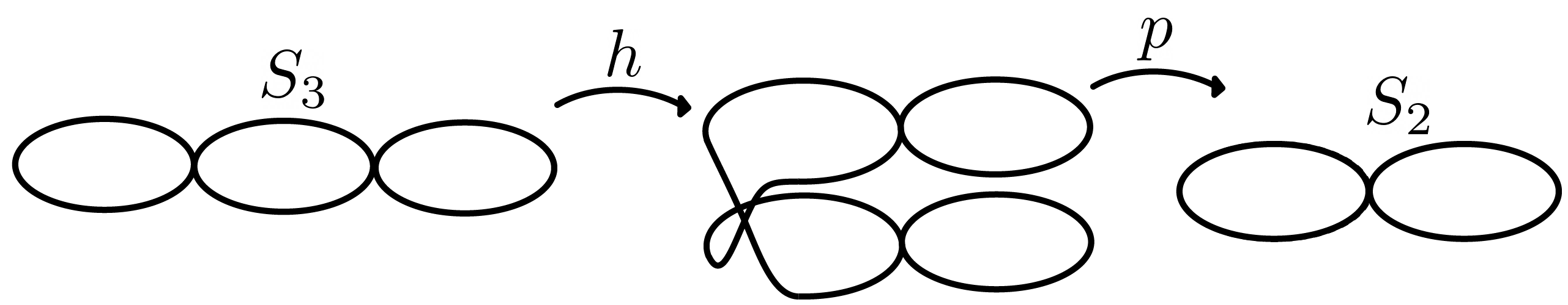
Figure 1: In the space $\mathbb{R}^{5}$ there is a genus three surface $\Sigma_{3}$ and in the space $\mathbb{R}^{3}$ there is a genus two surface $\Sigma_{2}$ such that projection $p_{3}:\mathbb{R}^{5}\to\mathbb{R}^{3}$ is a covering map (and thus a local diffeomorphism) $p_{3}:\Sigma_{3}\to\Sigma_{2}$. These surfaces can be obtained by taking curves that are deformed to surfaces by replacing all points of the curves by circles. The figure gives idea of the construction of such curves. In the figure we have a deformation $h:\mathbb{R}^{3}\to\mathbb{R}^{3}$ that maps a curve $S_{3}\subset\mathbb{R}^{3}$ to a self-intersecting curve $h(S_{3})\subset\mathbb{R}^{3}$ and projection $p:\mathbb{R}^{3}\to\mathbb{R}^{2}$ that maps $h(S_{3})$ to a curve $S_{2}\subset\mathbb{R}^{2}$. We add a forth dimension (time) in the space $\mathbb{R}^{3}$ that contains $S_{3}$, and modify $h$ in the time-variable to obtain a diffeomorphism $\tilde{h}:\mathbb{R}^{4}\to\mathbb{R}^{4}$ so that $\tilde{S}_{3}=\tilde{h}(S_{3}\times\{0\})$ is a non-self-intersecting by curve $\mathbb{R}^{4}$ which projetion to the 3-dimensional space $\mathbb{R}^{3}$ is $h(S_{3})$. We add one more dimension in all Euclidean spaces and obtain a diffeomorphism $\tilde{H}:\mathbb{R}^{4+1}\to\mathbb{R}^{4+1}$, $\tilde{H}(x,t)=(\tilde{h}(x),t)$ and the projection $p_{3}:\mathbb{R}^{4+1}\to\mathbb{R}^{2+1}$ such that $p_{3}\circ\tilde{H}:\tilde{S}_{3}\times\{0\}\to S_{2}\times\{0\}$. Finally, we replace all points of the curves by circles (analogously to the Penrose diagrams in general relativity) to deform the curves $\tilde{H}(\tilde{S}_{3})$ and $S_{2}\times\{0\}$ to surfaces $\Sigma_{2}\subset\mathbb{R}^{2+1}$ and $\Sigma_{3}\subset\mathbb{R}^{4+1}$ having the genus 2 and 3, respectively.

Example 1 (Examples of Homeomorphic and Locally Homeomorphic Manifolds).

Homeomorphisms preserve homotopy type so a surface of genus 3, $S_{3}$, and genus 2, $S_{2}$, are not homeomorphic. Nevertheless, there is e.g. a two-sheet covering of $S_{2}$ by $S_{3}$, and so there is a local homeomorphism from $S_{3}$ to $S_{2}$. A visualization of this covering is given in Figure 1. The covering is done in two steps, in the first the A local homeomorphism from $S_{3}$ to $S_{2}$ is given explicitly in Appendix B.2.

Lemma 1 and Corollary 1 show that limiting sequences of bistable uniform approximating sequences are always at least local homeomorphisms, and are in general weakly differentiable. A natural question is if they are always local diffeomorphisms. They are not. An example of a nonsmooth function that can be approximated bistably is given in Appendix B.4.

Any $C^{1}$ diffeomorphism can be uniformly approximated by $C^{\infty}$ diffeomorphisms [36, Theorem 2.7], hence uniform approximation results true of $C^{1}$ diffeomorphisms, are automatically true of $C^{\infty}$ ones as well. Further, from [61], we have that a homeomorphism can be uniformly approximated by a diffeomorphism if and only if the homeomorphism is isotopic to a diffeomorphism, as in the example given in Appendix B.4.

A limit homeomorphism $f_{\infty}$ of a sequence $(f_{i})$ is weakly differentiable in the Sobolev sense, see Corollary 4. The sign of the Jacobian determinant $\det Df_{\infty}$ carries topological information on the orientation of the mapping. Under weaker notions of converge this analytical information on the Jacobian determinant is lost. For example, by a result of Hencl and Vejnar [34], there exists a homeomorphism $f\colon\mathbb{R}^{4}\to\mathbb{R}^{4}$, which belongs to the Sobolev space $W^{1,1}$ but for which sets $\{\det Df>0\}$ and $\{\det Df<0\}$ have positive measure. This homeomorphism cannot be approximated by diffeomorphisms in the Sobolev norm of $W^{1,1}$. Indeed, if such an approximating sequence $(f_{i})$ would exist, then it would have a subsequence $(f_{i_{j}})$ having the property that $\det(Df_{i_{j}})\to\det(Df)$ almost everywhere, but this is not possible as functions $\det Df_{i_{j}}$ do not change sign.

The homeomorphism of Hencl and Vejnar is an intricate construction based on a reflection in a set containing a positive measure Cantor set and we do not discuss the construction of Hencl and Vejnar in more detail here. We merely note that homeomorphisms $f\times\rm{id}\colon\mathbb{R}^{4}\times\mathbb{R}^{k}\to\mathbb{R}^{4}\times\mathbb{R}^{k}$ for $k>0$ yield similar examples in all dimensions above four. In lower dimensions $n\leq 3$ construction of such homeomorphisms is not possible by a result of Hencl and Malý [33] which states that $W^{1,1}$-homeomorphisms in these dimensions have the property that their Jacobians do not change sign.

2.2 Measures on manifolds with nontrivial topology

The following result says that if we could get access to some manifold $\mathcal{M}_{1}$ which is homeomorphic to a target manifold $\mathcal{M}_{2}$, than we can learn to approximate measures on $\mathcal{M}_{2}$ using a network, under some dimension requirements.

Theorem 1.

Let $n_{0}=n,n_{L}=m$, $\mathcal{M}\subset\mathbb{R}^{n}$ be a compact $k$ manifold for $n\geq 3k+1$, $\mu\in\mathcal{P}(\mathcal{M}_{1})$, and be an absolutely continuous. Further let, for each $\ell=1,\dots,L$, $\mathcal{E}_{\ell}^{n_{\ell-1},n_{\ell}}\coloneqq\mathcal{T}^{n_{\ell}}_{\ell}\circ\mathcal{R}^{n_{\ell-1},n_{\ell}}_{\ell}$ for $\ell=1,\dots,L$, where $n_{\ell}\geq 3n_{\ell-1}+1$, $\mathcal{R}^{n_{\ell-1},n_{\ell}}_{\ell}\subset C^{1}(\mathbb{R}^{n_{\ell-1}},\mathbb{R}^{n_{\ell}})$ is a family of injective maps that contains a linear map and the families $\mathcal{T}^{n_{\ell}}_{\ell}$ are dense in $\hbox{Diff}^{2}(\mathbb{R}^{n_{\ell}})$ (e.g., $\mathcal{T}^{n_{\ell}}_{\ell}$ is a family of bijective networks [71, Section 2]). Finally let $\mathcal{T}^{n}_{0}\subset\hbox{Diff}^{2}(\mathbb{R}^{n_{0}})$ be distributionally universal family and $f\in\operatorname*{emb}^{1}(\mathcal{M}_{1},\mathbb{R}^{m})$. Then, there is a sequence of $\left\{E_{i}\right\}_{i=1,2,\dots}\subset\mathcal{E}_{L}^{n_{L-1},m}\circ\dots\circ\mathcal{E}_{1}^{n_{1},n}\circ\mathcal{T}^{n}_{0}$ such that

$$\lim_{i\to\infty}\operatorname{W}_{2}\left({f}{}_{\#}{\mu},{E_{i}}{}_{\#}{\mu}\right)=0.$$ (3)

The proof of Theorem 1 is given in the Appendix in B.5. This theorem has the following corollary that says that, morally, the generative problem of learning a $\nu$ with support $\mathcal{M}_{2}$ can be solved if we had access to a $\mathcal{M}_{1}$ diffeomorphic to $\mathcal{M}_{2}$.

Corollary 2.

Let $\nu$ be a Borel measure in $\mathbb{R}^{m_{2}}$ which support is a subset of some smooth compact $n$ submanifold $\mathcal{M}_{2}$ of $\mathbb{R}^{m_{2}}$ and let $\nu$ be absolutely continuous w.r.t. Riemannian measure of $\mathcal{M}_{2}$. If a submanifold $\mathcal{M}_{1}$ in $\mathbb{R}^{m_{2}}$ is smooth and diffeomorphic to $\mathcal{M}_{2}$ for $m_{1}\gg n$ and $m_{2}\gg n$, then the Trumpet architecture [48] pushes forward the uniform distribution on $\mathcal{M}_{1}$ arbitrarily close to $\nu$ in Wasserstein distance.

The 0proof of Corollary 2 is given in the Appendix in B.6. This corollary says that one can use existing architectures, e.g. [48], to solve generation problems, provided that we know the topology of $\mathcal{M}_{2}$, so that we can construct a suitable $\mathcal{M}_{1}$. In this sense, although the embedding of $\mathcal{M}_{2}$ doesn’t need to be known exactly, its topology must be completely understood. Furthermore, provided we can obtain universality with respect to the relevant function classes, than we can get universality in the sense of pushforward of measure.

Corollary 3 (Bistable Uniform Approximation Implies Pushforward Universality).

Let $m_{2}\geq 3n+1$, $\mathcal{M}_{1}\subset\mathbb{R}^{m_{1}},\mathcal{M}_{2}\subset\mathbb{R}^{m_{2}}$, and let $\mathcal{F}\subset\operatorname{locdif}^{1}(\mathcal{M}_{1},\mathbb{R}^{m_{2}})$ be a bistable uniform approximator for $\mathcal{G}\subset C(\mathcal{M}_{1},\mathcal{M}_{2})$. Then for any $\mu\in\mathcal{P}(\mathcal{M}_{1})$ absolutely continuous and $g\in\mathcal{G}$, there is a sequence $\left(f{}_{i}\right)^{\infty}_{i=1}\subset\mathcal{F}$ so that $\lim_{i\to\infty}\operatorname{W}_{2}\left({g}{}_{\#}{\mu},{f_{i}}{}_{\#}{\mu}\right)=0$.

The proof of Corollary 3 is given in the Appendix in B.7. The above results show that if $\mathcal{T}\circ p\circ\mathcal{E}$ is a bistable uniform approximator to $\mathcal{F}$, then questions of learning to approximate measures supported on $\operatorname*{Range}(f)$ for $f\in\mathcal{F}$ are solved. Thus, for the remainder of the section, we focus on the problem of showing that $\mathcal{T}\circ p\circ\mathcal{E}$ is a bistable uniform approximator with respect to the largest class $\mathcal{F}$ possible.

2.3 Covering maps and learning topology

Here we present a topological theorem. This result has a technical appearance, but is the major work horse for the subsequent developments in the paper.

Theorem 2 (Covering Map Decomposition).

Let $\mathcal{M}_{1}\subset\mathbb{R}^{m_{1}}$ and $\mathcal{M}_{2}\subset\mathbb{R}^{m_{2}}$ be smooth compact $n$-manifolds, where $\mathcal{M}_{2}$ is triangulable, and let $p\colon\mathbb{R}^{m_{2}}\times\mathbb{R}^{2n+1}\to\mathbb{R}^{m_{2}}$ be the projection to the first coordinate. Then each local diffeomorphism $g\colon\mathcal{M}_{1}\to\mathcal{M}_{2}$ there exists an embedding $h\colon\mathcal{M}_{1}\to\mathcal{M}_{2}\times\mathbb{R}^{2n+1}$ for which $g=p\circ h$ and so that the restriction $p|_{h(\mathcal{M}_{1})}\colon h(\mathcal{M}_{1})\to\mathcal{M}_{2}$ is a covering map. Moreover, if $\mathcal{M}_{2}$ is given a triangulation $K$ that is fine enough, then we may fix $h$ satisfying the following condition: for each vertex $v$ of the triangulation $K$, the preimage $p^{-1}(v)$ is $\{v\}\times\{0,1\ldots,d\}\times\{0\}^{2n}$, where $d$ is the degree of the map $g$.

The proof of Theorem 2 is given in the Appendix in B.8. A difficulty in proving Theorem 2 is that $p$ is not merely a map between abstract spaces, but rather a projector in the ambient space. The fact that such a projector exists is non-obvious when $\mathcal{M}_{1}$ or $\mathcal{M}_{2}$ are, for example, knotted.

Theorem 2 allows us to approximate a local diffeomorphism $g$ by approximating $h$, a diffeomorphism. We can then compose this approximation with a projection $p$ which only depends on the degree of $g$. This leads to the following theorem.

Theorem 3 (Bistable Approximations of Local Diffeomorphisms).

Let $\mathcal{M}_{1}\subset\mathbb{R}^{m_{1}}$ and $\mathcal{M}_{2}\subset\mathbb{R}^{m_{2}}$ be compact submanifolds, $m_{2}\geq 3n+1$, $\mathcal{E}\subset\operatorname*{emb}^{1}\left(\mathcal{M}_{1},\mathbb{R}^{m_{2}+2n+1}\right)$ be a uniformly bistable approximator of each smooth embedding $h\colon\mathcal{M}_{1}\to\mathbb{R}^{m_{2}+2n+1}$, and $\mathcal{T}\subset\operatorname{dif}^{1}\left(\mathbb{R}^{m_{2}},\mathbb{R}^{m_{2}}\right)$ be a uniformly bistable approximator of $\operatorname{dif}^{1}(\mathbb{R}^{m_{2}},\mathbb{R}^{m_{2}})$. Then, for any $g:\mathcal{M}_{1}\to\mathcal{M}_{2}$, and finite $Y\subset\mathcal{M}_{2}$, there is a bistable uniform approximating sequence $\left(f{}_{i}\right)^{\infty}_{i=1}\subset\mathcal{T}\circ p\circ\mathcal{E}$ for $g$. Further, if the degree of $g$ is $d$ then for $f_{i}=T_{i}\circ p\circ E_{i}$, the set

$$X_{i}\coloneqq\left\{\operatornamewithlimits{argmin}_{x\in\mathcal{M}_{1}}\lVert E_{i}(x)-(T_{i}^{-1}(y),j,\left\{0\right\}^{2n})\rVert_{2}\colon y\in Y,j\in\left\{1,\dots,d\right\}\right\}$$ (4)

satisfies

$$d_{H}(X_{i},g^{-1}(Y))\to 0$$ (5)

as $i\to\infty$ where $d_{H}$ is the Hausdorff distance.

The proof of Theorem 3 is given in the Appendix in B.9. The set $X_{i}$ defined in Eqn. 4 can be computed in closed-form provided that $E_{i}$ and $T_{i}$ admit closed-form inverses. This, combined with Eqn. 5, means that we can compute arbitrarily good approximations to the multi-values inverses of $g$ on any point in $Y$. Theorem 3 says that local diffeomorphisms can always be learned in a bistable way using expansive-projectors. What about manifolds that don’t admit local diffeomorphisms? We explore this question in the following

Corollary 4 (Approximations to Maps Between Non Locally Homeomorphic Manifolds).

Let $\mathcal{M}_{1}\subset\mathbb{R}^{m_{1}}$ and $\mathcal{M}_{2}\subset\mathbb{R}^{m_{1}}$ be smooth compact manifolds, and $\operatorname{lochom}(\mathcal{M}_{1},\mathcal{M}_{2})$ be empty. Let $g\colon\mathcal{M}_{1}\to\mathcal{M}_{2}$ be continuous and surjective. There are no bistable uniform approximating sequences of $g$.

The proof of Corollary 4 is given in the Appendix in B.10. Corollary 4 shows that the only functions between smooth compact manifolds that can be approximated bistably (by anything) but are not approximated by the network lie in $\operatorname{lochom}(\mathcal{M}_{1},\mathcal{M}_{2})\setminus\operatorname{locdif}(\mathcal{M}_{1},\mathcal{M}_{2})$.

3 Applications and Implications

In this section, we describe how the networks studied in this work are naturally connected to various other problems in machine learning, as well as an application in cryo-EM.

3.1 Group Invariant Networks

Let $\Sigma$ be a group with action $g_{\sigma}\colon\mathcal{M}_{1}\to\mathcal{M}_{1}$ for each $\sigma\in\Sigma$. When constructing a group invariant network $E\colon\mathcal{M}_{1}\to\mathcal{M}_{2}$, the task is to approximate an $f\colon\mathcal{M}_{1}\to\mathcal{M}_{2}$ by building a network (via choice of architecture or else averaged training) so that $E(g_{\sigma}x)=E(x)$ for all $\sigma\in\Sigma$ and $x\in\mathcal{M}_{1}$. If $f$ is $\Sigma$ invariant as well then enforcing $\Sigma$ invariance of $E$ does not harm approximation and improves both training and generalization error in theory [10] and in practice [18].

For each $x\in\mathcal{M}_{1}$ we call the orbit of $x$ the set $\text{orbit}(x)\coloneqq\left\{g_{\sigma}x\colon\sigma\in\Sigma\right\}$. We let $\mathcal{M}_{1}/\Sigma$ denote the quotient of $\mathcal{M}_{1}$ by the group action, that is, the orbit space of $\mathcal{M}_{1}$ by $\Sigma$. A group on $\mathcal{M}$ is called free if for any $x\in\mathcal{M}_{1}$, $g_{\sigma}x=x$ implies that $\sigma$ is the identity. It is called smooth if the map $g_{\sigma}(x)$ is smooth as a function of $x$ for each $\sigma\in\Sigma$. If a finite $\Sigma$ is smooth and free, then $\mathcal{M}_{1}/\Sigma$ is a smooth manifold [53, Theorem 21.13]. This suggests that there is a connection between learning $f\colon\mathcal{M}_{1}\to\mathcal{M}_{2}$ that is $\Sigma$ invariant, and learning a ‘symmetrized’ modification of $f$ defined between $\colon\mathcal{M}_{1}/\Sigma\to\mathcal{M}_{2}$. When the group action induces constant-sized orbits (a stronger condition than $\Sigma$ acting freely) then this is indeed the case.

Lemma 2 (Symmetrization as a Quotient Manifolds).

Let $\Sigma$ be a continuous finite group on compact $n$ manifold $\mathcal{M}_{1}$ so that the orbit of $x$ is the same size for all $x\in\mathcal{M}_{1}$, and let $f\colon\mathcal{M}_{1}\to\mathcal{M}_{2}$ be a continuous $\Sigma$ invariant smooth map. Then the quotient space $\mathcal{M}_{1}/\Sigma$ is an $n$ manifold,

1. let $\pi_{\Sigma}\colon\mathcal{M}_{1}\to\mathcal{M}_{1}/\Sigma$ take each point to its orbit and ${\left.\kern-1.2ptf\vphantom{\big{|}}\right|_{\mathcal{M}_{1}/\Sigma}}\colon\mathcal{M}_{1}/\Sigma\to\mathcal{M}_{2}$ so that ${\left.\kern-1.2ptf\vphantom{\big{|}}\right|_{\mathcal{M}_{1}/\Sigma}}(\text{orbit}(x))=f(x)$, then

   $$f={\left.\kern-1.2ptf\vphantom{\big{|}}\right|_{\mathcal{M}_{1}/\Sigma}}\circ\pi_{\Sigma},$$ (6)

2. if both $f$ and $\Sigma$ are smooth, $f$ is surjective and $d$-to-one where $\left\lvert\Sigma\right\rvert=d$, then $f\in\operatorname{locdif}(\mathcal{M}_{1},\mathcal{M}_{2})$.

The proof of Lemma 2 is given in the Appendix in B.11. The r.h.s. of Eqn. 6 can be used to construct a $\Sigma$ invariant network in general. See, e.g. the symmetrization operator studied in [11, Sec. 3.4] or group convolution [13, Sec. 4.3], both of which play a similar role to the $\pi_{\Sigma}$ here.

The final point of Lemma 2 gives conditions under which a $\Sigma$ invariant function $g$ is a local diffeomorphism and so can be approximated bistably by the networks considered here. Combining this with Theorem 3 yields a result that says that we can back out the group action of $\Sigma$ from the $g$ approximation, without knowledge of $\Sigma$. The proof of Corollary 5 is given in the Appendix in B.12.

Corollary 5 (Recovery of Group Action).

Let $h\colon\mathcal{M}_{1}\to\mathcal{M}_{2}$ be a smooth, surjective, $d$-to-one, $\Sigma$ invariant function for $n$ submanifolds $\mathcal{M}_{1}\subset\mathbb{R}^{m_{1}}$ and $\mathcal{M}_{2}\subset\mathbb{R}^{m_{2}}$, and let $Y\subset\mathcal{M}_{2}$ be finite. Then there is a sequence $\left(f{}_{i}\right)^{\infty}_{i=1}\subset\mathcal{T}\circ p\circ\mathcal{E}$ that is a bistable uniform approximator for $h$, and for each $y\in Y$, $f_{i}^{-1}(y)$ converges to a $\Sigma$ orbit in Hausdorff distance.

3.2 Choice of Starting Space

In a generation problem, the goal is to approximate a probability distribution $\nu$ over some subset $\mathcal{X}$ of $\mathbb{R}^{m}$ given samples $X$ from $\nu$. This can be solved by fixing a base distribution $q$ over some simpler subset $\mathcal{Z}$ of $\mathbb{R}^{n}$ and using a neural network to learn $f\colon\mathbb{R}^{n}\to\mathbb{R}^{m}$ so that ${f}{}_{\#}{q}\approx\nu$ [12, 14, 20, 30, 49, 66, 67, 75, 78]. This leads to the question: how should we choose $\mathcal{Z}$ to allow for maximal flexibility of $\mathcal{X}$?

The classification theorem [62, Theorem 77.5] says that each connected compact $2$ manifolds is homeomorphic to $S^{2}$, the $n$-fold torus, or the $m$-fold projective plane. Further, orientable surfaces can be classified by genus alone while a nonorientable surface is covered by its orientation covering [53, Theorem 15.41] itself an orientable surface. Moreover, by [32, Example 1.41 and Page 157], there exists some covering map from an oriented Riemannian surface $S_{m}$ of genus $m$ to an oriented Riemannian surface $S_{n}$ of genus $n$ if and only if $m=(n-1)k+1$, as the following lemma shows.

Lemma 3 (Local Diffeomorphisms Between Surfaces).

Let $m=(n-1)k+1$, where $n,m,k\in\mathbb{Z}_{+}$, $k\geq 2$ and $d\geq 5$. Moreover, let $S_{n}$ and $S_{m}$ be oriented Riemannian surface of genus $n$ and $m$, respectively. Then $S_{n}$ and $S_{m}$ can be embedded in $\mathbb{R}^{d}$ so that the restriction of the projection $p:\mathbb{R}^{3}\times\mathbb{R}^{d-3}\to\mathbb{R}^{3},$ $p(x,y)=x$ defines a $k$-to-1 covering map $p|_{S_{m}}:S_{m}\to S_{n}$. In particular, $p|_{S_{m}}:S_{m}\to S_{n}$ is a surjective local diffeomorphism.

The proof of Lemma 3 is given in the Appendix in B.13. This shows that such a covering map exists, however the existence of such a covering map does not guarantee that if $S_{n}$ and $S_{m}$ are submanifold of an Euclidean space that the covering map extends to continuous map of the Euclidean space. In the next lemma we prove when $S_{n}$ and $S_{m}$ are embedded in the Euclidean space appropriately, the covering map is realized by projection.

This lemma can be combined with the following theorem which gives a general construction for local diffeomorphisms using projectors between manifolds $\mathcal{M}_{1}$ and $\mathcal{M}_{2}$ by passing through diffeomorphisms.

Theorem 4 (Covering Maps as Projections).

Let $\mathcal{M}_{1}\subset\mathbb{R}^{m_{1}}$, $\mathcal{M}_{2}\subset\mathbb{R}^{m_{2}}$, $\tilde{\mathcal{M}}_{1}\subset\mathbb{R}^{\tilde{m}_{1}}$ and $\tilde{\mathcal{M}}_{2}\subset\mathbb{R}^{\tilde{m}_{2}}$ be compact smooth submanifolds where $\tilde{m}_{1}>m_{1}$ and $\tilde{m}_{2}>m_{2}$. Suppose further that both $\mathcal{M}_{1}$ and $\tilde{\mathcal{M}}_{1}$ as well as $\mathcal{M}_{2}$ and $\tilde{\mathcal{M}}_{2}$ are diffeomorphic and there is a projection $p\colon\mathbb{R}^{\tilde{m}_{1}}\to\mathbb{R}^{\tilde{m}_{2}}$ so that the restriction of $p|_{\tilde{\mathcal{M}}_{1}}$ is a covering map $p|_{\tilde{\mathcal{M}}_{1}}:\tilde{\mathcal{M}}_{1}\to\tilde{\mathcal{M}}_{2}$. Then there is a linear injective map $J_{1}\colon\mathbb{R}^{m_{1}}\to\mathbb{R}^{\tilde{m}_{1}}$, a diffeomorphism $T_{1}\colon\mathbb{R}^{\tilde{m}_{1}}\to\mathbb{R}^{\tilde{m}_{1}}$, an integer $k\geq\max(\tilde{m}_{2},3m_{2}+1)$, a linear injective map $J_{2}\colon\mathbb{R}^{\tilde{m}_{2}}\to\mathbb{R}^{k}$, a diffeomorphism $T_{2}\colon\mathbb{R}^{k}\to\mathbb{R}^{k}$, and a projection $p_{2}\colon\mathbb{R}^{k}\to\mathbb{R}^{m_{2}}$ such that $f=p_{2}\circ T_{2}\circ J_{2}\circ p\circ T_{1}\circ J_{1}\in\operatorname{locdif}(\mathcal{M}_{1},\mathcal{M}_{2})$ is a $k$-to-1 covering map $f:\mathcal{M}_{1}\to\mathcal{M}_{2}$.

The proof of Theorem 4 is given in the Appendix in B.14. Theorem 4 gives a recipe for extending this to the case when $S_{3}$ is a surface with two knotted handles, that is a torus that is embedded in expansive-projectors non-standard [68]. As products of covering maps are a covering map, Theorem 4 and Lemma 3 imply the following. Let $m=k!+1$, $N\subset\mathbb{R}^{d_{1}}$ be a compact connected submanifold and $S_{m}\subset\mathbb{R}^{d_{2}}$ be an oriented Riemannian surface of genus $m$. Next, we consider the model space $N\times S_{m}\subset\mathbb{R}^{m_{1}}$, $m_{1}=d_{1}+d_{2}$ and its possible images in the composition networks of the form Eq. 1. Let $\mathcal{M}_{2}\subset\mathbb{R}^{m_{2}}$ be a submanifold that that is diffeomorphic to $N\times S_{n}$, where $S_{n}$ is an oriented Riemannian surface of genus $n$ with $n\leq k+1$. Then by Theorem 4 there is a composition $f:=p_{2}\circ T_{2}\circ J_{2}\circ p\circ T_{3}\circ J_{3}:\mathbb{R}^{m_{1}}\to\mathbb{R}^{m_{2}}$ of projections, global diffeomorphisms and linear injective maps such that $f:N\times S_{m}\to N\times S_{n}$ is a surjective local diffeomophism. This means that a combination of two composition networks of the form Eq. 1 can can map the model manifold $N\times S_{m}$ to any manifold diffeomorphic to $N\times S_{n}$ with $n\leq k+1$. In particular, if we consider the first betting number $b_{1}(N)$ of the manifold $N$ (i.e. the number of handles), the composition map $f$ can map $N\times S_{n}$ to manifolds having any 1st Betti number $n\cdot b_{1}(N)$ with $n\leq k+1$.

3.3 Cryogenic Electron Microscopy

Cryogenic electron microscopy (cryo-EM) is a molecular imaging technique where samples (molecules) are suspended in vitreous ice and tomographically imaged with an electron microscope (2017 Nobel Prize in Chemistry). Like in traditional tomography one images the three-dimensional sample with two-dimensional projections (slices) but with unknown orientations. Orientations are then modeled as random samples from the rotation group $\mathrm{SO}(3)$, often from the Haar (uniform) measure [8, 29]. The task is to recover the underlying molecular density up to natural global symmetries. Mathematically, this can be modeled as the problem of recovering the orbit of samples under the rotation group, $\mathrm{SO}(3)$ [55].

In addition to the emergence of $\mathrm{SO}(3)$ as a natural group in this problem, the molecule often has its own discrete symmetries which means that the orbit to recover is topologically different from $\mathrm{SO}(3)$. The presence of a symmetry in the sample, encoded by a group $\Sigma$, means that the natural problem is to recover orbits of $\mathrm{SO}(3)/\Sigma$, where $\Sigma$ is unknown. This task is a natural setting for the analysis in this manuscript, see Lemma 2 and Theorem 5.

We remark that the results described in Section 3.1 apply only when $\Sigma$’s group action produces orbits of constant size. This is not the case for some natural settings. Indeed in the setting of imaging a bacteriophage, rotation out the axis of symmetry fixes the points at the poles, and so is not free. Thus, quotients of manifolds by $\Sigma$ do not yield manifolds, but so-called orbifolds [85, Chapter 13]. Extending the analysis of the manuscript to apply to the case when the target space is an orbifold will be the subject of future work.

4 Conclusion

In this work we showed that extension-projection networks are universal approximators of local diffeomorphisms between smooth compact manifolds. In particular, we showed that we can approximate mappings that globally change topology between manifolds. We found that local diffeomorphisms can always be lifted to diffeomorphisms in a sufficiently high dimensional space. By approximating this lifting and a subsequent projection, we found that extension-projection networks are end-to-end universal approximators of local diffeomorphisms while maintaining a novel inversion property. Finally, we considered applications where our extension-projection networks can be used.

5 Acknowledgements

M.P. was supported by the CAPITAL Services. M.L. was supported by Academy of Finland, grants 284715, 312110. P.P. was supported by Academy of Finland grant 332671. I.D. was supported by the European Research Council Starting Grant 852821—SWING. M.V. dH. gratefully acknowledges support from the Department of Energy under grant DE-SC0020345, the Simons Foundation under the MATH + X program, and the corporate members of the Geo-Mathematical Imaging Group at Rice University.

Appendix A Definition of Terms

A Hausdorff space is a topological space so that distinct points are always separated by disjoint neighborhoods. Metric spaces are always Hausdorff, and so is $\mathbb{R}^{n}$ with the usual metric.

A $n$ manifold, notated $\mathcal{M}$, is a Hausdorff space with countable basis such that each point $x$ in $\mathcal{M}$ has a neighborhood that is homeomorphic with an open subset of $\mathbb{R}^{n}$.

A $n$ submanifold is a manifold that is embedded in $\mathbb{R}^{m}$ for some $m$.

Given two topological spaces $X$ and $Y$, we notate $\hom(X,Y)$ as the space of homeomorphisms between $X$ and $Y$. That is, the set of functions $X\to Y$ which are continuous and bijective with continuous inverse.

Given two topological spaces $X$ and $Y$, we notate $\operatorname{lochom}(X,Y)$ as the space of local homeomorphisms between $X$ and $Y$. That is, the set of functions $f\colon X\to Y$ so that $f$ maps open subsets of $X$ to open subsets of $Y$ and for every $x\in X$, there is an open neighborhood $U\subset X$ so that ${\left.\kern-1.2ptf\vphantom{\big{|}}\right|_{U}}\colon U\to f(U)$ is a homeomorphism. Observe that if $X$ is compact and non-empty and $Y$ is connected, then all local homeomorphism $f:X\to Y$ are surjective maps.

Given a Riemannian $n$ manifold $\mathcal{M}$ we use the notation $d_{\mathcal{M}}(\cdot,\cdot)$ to refer to the geodesic metric.

Given two $n$ manifolds with geodesic metrics $\mathcal{M}_{1}$ and $\mathcal{M}_{2}$, we notate $\operatorname{locbilip}(\mathcal{M}_{1},\mathcal{M}_{2})$ as the space of locally bilipschitz functions $f\colon\mathcal{M}_{1}\to\mathcal{M}_{2}$ which are local homeomorphisms and for which there is an $L>0$ so that for all $x\in\mathcal{M}_{1}$ there is an open $U_{x}\subset\mathcal{M}_{1}$ so that for all $x^{\prime}\in U_{x}$ $\frac{1}{L}d_{X}(x,x^{\prime})\leq d_{Y}(f(x),f(x^{\prime}))\leq Ld_{X}(x,x^{\prime})$.

Given two smooth manifolds $X$ and $Y$, a smooth map $f\colon X\to Y$ is a diffeomorphims if it is bijection and its inverse is a smooth map. We denote $\operatorname{dif}(X,Y)$ as the space of diffeomorphisms between $X$ and $Y$. Moreover, we notate $\operatorname{locdif}(X,Y)$ as the space of local diffeomorphisms between $X$ and $Y$. That is, the set of functions $f\colon X\to Y$ so that $f$ maps open subsets of $X$ to open subsets of $Y$ and for every $x\in X$, there is an open neighborhood $U\subset X$ so that ${\left.\kern-1.2ptf\vphantom{\big{|}}\right|_{U}}\colon U\to f(U)$ is a diffeomorphism. All local diffeomorphism are local homeomorphism and thus, if $X$ is compact and non-empty and $Y$ is connected, then all local diffeomorphism $f:X\to Y$ are surjective maps.

We call a function $f$ an embedding and denote it by $f\in\operatorname*{emb}(X,Y)$ if $f:X\to Y$ is continuous, injective, and $f^{-1}\colon f(X)\to X$ is continuous. Also we denote by $\operatorname*{emb}^{k}(\mathbb{R}^{n},\mathbb{R}^{m})$ the set of maps $f\in\operatorname*{emb}(\mathbb{R}^{n},\mathbb{R}^{m})\cap C^{k}(\mathbb{R}^{n},\mathbb{R}^{m})$ which differential $df|_{x}:\mathbb{R}^{n}\to\mathbb{R}^{m}$ is injective at all points $x\in\mathbb{R}^{n}$.

Given a smooth $n$ manifold and point $x\in\mathcal{M}$, $T_{x}\mathcal{M}$ denotes the tangent space of $\mathcal{M}$ at $x$. $T\mathcal{M}$ denotes the tangent space of $\mathcal{M}$.

Two homeomorphisms $\phi$ and $\psi$ are said to be isotopic if there exists a continuous $\Phi\colon[0,1]\times\mathcal{M}\to\mathcal{M}$ so that $\Phi(t,\cdot)$ is a homeomorphism for each $t$, and so that $\Phi(0,\cdot)=\phi$, and $\Phi(1,\cdot)=\psi$.

Let $X$ be a topological space. We call $X$ a polyhedron if there exists a simplicial complex $K$ and a homeomorphism $h\colon\left\lvert K\right\rvert\to X$. The pair $(K,h)$ is called a triangulation of $X$. For a well-written, high level description of triangulation of manifolds, see [57] or [73, Chapter 7]. A key result is that all smooth topological manifolds are triangulable. Further, every topological $n$ manifold is triangulable if $n<4$, but counter examples exist for $n\geq 4$.

In Definition 1, $\left(\nabla f(x)\right)^{-1}$ refers to the inverse of a gradient matrix, not the gradient of the inverse mapping. Similarly the norm $\lVert\cdot\rVert_{T_{x}\mathcal{M}_{1}\times{\mathbb{R}^{m_{2}}}}$ denotes, e.g., the operator (matrix) norm.

Appendix B Proofs

B.1 Helper Lemma

Before we proceed with the proof of our main results, we first present the following helper lemma, which allows us to compare the euclidian distance between points with the geodesic distance. It lets us compare euclidian distance (as vectors in $\mathbb{R}^{m}$) and arclength geodesic distances (as points on an $n$-manifold $\mathcal{M}$) between two points. This presentation and Lemma are not original, and are taken from [9, Section 3].

Let $\mathcal{M}$ be a smooth $n$ manifold embedded in $\mathbb{R}^{m}$. We define the minimum radius of curvature $r_{0}(\mathcal{M})$ as

$$\frac{1}{r_{0}(\mathcal{M})}=\max_{\gamma,t}\lVert\ddot{\gamma}(t)\rVert_{\mathbb{R}^{n}}$$

where $\gamma\colon D\to\mathbb{R}^{m}$ varies over all unit-sphere geodesics in $\mathcal{M}$, and $t$ varies over $D$. The minimum branch separation $s_{0}(\mathcal{M})$ is the largest positive number for which

$$\lVert x-y\rVert_{\mathbb{R}^{m}}<s_{0}(\mathcal{M})\text{ implies that }d_{\mathcal{M}}(x,y)\leq\pi r_{0}(\mathcal{M}).$$

Lemma 4 (Comparing Euclidian and Geodesic Distances).

Let $\mathcal{M}$ be a smooth compact $n$ manifold that connects points $x$ and $y$ with geodesic $\gamma$ of length $\ell$. Then $r_{0}(\mathcal{M})>0$ and $s_{0}(\mathcal{M})>0$ both exist. Further, if $\ell\leq\pi r_{0}(\mathcal{M})$, then

$$2r_{0}(\mathcal{M})\sin(\ell/2r_{0}(\mathcal{M}))\leq\lVert x-y\rVert_{\mathbb{R}^{m}}\leq\ell.$$

The Lemma above is the same as in [9, Lemma 3]. We refer the reader to that work for a proof. If we denote the geodesic distance $d_{\mathcal{M}}\colon\mathcal{M}\times\mathcal{M}\to\mathbb{R}$ as

$$d_{M}(x,y)\coloneqq\inf_{\gamma}\left\{\text{length}\left(\gamma\right)\right\}$$

where $\gamma$ varies over the smooth paths connecting $x$ and $y$, then Lemma 4 implies that when $d_{\mathcal{M}}(x,y)\leq\pi r_{0}(\mathcal{M})$,

$$(2/\pi)d_{\mathcal{M}}(x,y)\leq\lVert x-y\rVert_{\mathbb{R}^{m}}\leq d_{\mathcal{M}}(x,y).$$ (7)

When $\mathcal{M}$ is compact, this implies that there is a constant $c_{\mathcal{M}}>0$ such that for all $x,y\in\mathcal{M}$,

$$c_{\mathcal{M}}d_{\mathcal{M}}(x,y)\leq\lVert x-y\rVert_{\mathbb{R}^{m}}\leq d_{\mathcal{M}}(x,y).$$ (8)

B.2 Proof Of Lemma 1

In this subsection we present the proof of Lemma 1.

Proof.

Let $\left(f{}_{n}\right)^{\infty}_{n=1}$ be a bistable uniform approximating sequence converging to $g\colon\mathcal{M}_{1}\to\mathbb{R}^{m_{2}}$. We first show that $g$ is Lipschitz, and inverse Lipschitz when restricted to a small metric ball.

Let $x_{1},x_{2}\in\mathcal{M}_{1}$ be given, and close enough together so that Eqn. 7 applies. Then for any $n$, we have that

$$d_{\mathcal{M}_{2}}(g(x_{1}),g(x_{2})) \leq\pi/2\lVert g(x_{1})-f_{n}(x_{1})\rVert_{\mathbb{R}^{m}}+\pi/2\lVert g(x_{2})-f_{n}(x_{2})\rVert_{\mathbb{R}^{m}}+d_{Y_{n}}(f_{n}(x_{1}),f_{n}(x_{x}))$$

$$\leq\pi M/2d_{X}(x_{1},x_{2})+\pi\epsilon_{n}$$

where $Y_{n}$ denotes the manifold $f_{n}(\mathcal{M}_{1})$. If we let $n\to\infty$ then $n\to 0$, and so $\lVert g(x_{1})-g(x_{2})\rVert\leq M\lVert x_{1}-x_{2}\rVert$. Thus $g$ is Lipshitz with constant $\pi M/2$.

Now we prove that $g$ is locally inverse Lipschitz. Let $n\in\mathbb{Z}_{+}$ and $x_{0}\in\mathcal{M}_{1}$. As $\lVert\left(\nabla({P_{\mathcal{M}_{2}}\circ f_{n})}(x_{0})\right)^{-1}\rVert_{T_{{P_{\mathcal{M}_{2}}\circ f_{n}}(x_{0})}\mathcal{M}_{2}\times T_{x}\mathcal{M}_{1}}\leq M$, the inverse function theorem (see e.g. [82, Theorem 17.7.2]) implies that there is some neighborhood $V\subset\mathcal{M}_{1}$ of $x_{0}$ so that ${\left.\kern-1.2pt{P_{\mathcal{M}_{2}}\circ f_{n}}\vphantom{\big{|}}\right|_{V}}\colon V\to W={P_{\mathcal{M}_{2}}(f_{n}(V))}$ is a bijection and has a $C^{1}$-smooth inverse $h_{n,V}:({\left.\kern-1.2ptP_{\mathcal{M}_{2}}\circ f_{n}\vphantom{\big{|}}\right|_{V}})^{-1}:W\to V$ such that the norm of derivative of $h_{n,V}$ is bounded by $M$. Consider now $x_{1},x_{2}\in\mathcal{M}_{1}$. Consider the geodesic $\gamma$ of $\mathcal{M}_{2}$ that connects $y_{1}=P_{\mathcal{M}_{2}}\circ f_{n}(x_{1})$ to $y_{2}=P_{\mathcal{M}_{2}}\circ f_{n}(x_{2})$. By covering the geodesic $\gamma$ by neighborhoods $V_{j}$ where the inverse map $h_{n,V_{j}}$ are defined, we see that

$$d_{\mathcal{M}_{1}}(x_{1},x_{2})\leq Md_{\mathcal{M}_{2}}(P_{\mathcal{M}_{2}}\circ f_{n}(x_{1}),P_{\mathcal{M}_{2}}\circ f_{n}(x_{2})).$$

Next, let $x_{1},x_{2}\in\mathcal{M}_{1}$ and assume the $\epsilon_{n}$ is so small that $\epsilon_{n}<\hbox{reach}(\mathcal{M}_{2})/2$. Then,

$$\lVert{P_{\mathcal{M}_{2}}\circ f_{n}(x_{1})-P_{\mathcal{M}_{2}}\circ f_{n}(x_{2})}\rVert \geq c_{\mathcal{M}_{2}}d_{\mathcal{M}_{2}}(P_{\mathcal{M}_{2}}\circ f_{n}(x_{1}),P_{\mathcal{M}_{2}}\circ f_{n}(x_{2}))$$

$$\geq c_{\mathcal{M}_{2}}M^{-1}d_{\mathcal{M}_{1}}(x_{1},x_{2})$$

$$\geq c_{\mathcal{M}_{2}}M^{-1}\lVert x_{1}-x_{2}\rVert$$

Recall that by the definition of $P_{\mathcal{M}_{2}}$, the point $P_{\mathcal{M}_{2}}\circ f_{n}(x)$ is the nearest point of $\mathcal{M}_{2}$ to $f_{n}(x)$. Hence, as $|f_{n}(x)-g(x)|<\epsilon_{n}$ and $g(x)\in\mathcal{M}_{2}$, we have

$$|f_{n}(x)-P_{\mathcal{M}_{2}}\circ f_{n}(x)|\leq|f_{n}(x)-g(x)|<\epsilon_{n}.$$

Hence,

$$\lVert{f_{n}(x_{1})-f_{n}(x_{2})}\rVert\geq\lVert{P_{\mathcal{M}_{2}}\circ f_{n}(x_{1})-P_{\mathcal{M}_{2}}\circ f_{n}(x_{2})}\rVert-2\epsilon_{n}\geq c_{\mathcal{M}_{2}}M^{-1}\lVert x_{1}-x_{2}\rVert-2\epsilon_{n}.$$

Then we have

$$d_{\mathcal{M}_{2}}(g(x_{1}),g(x_{2})) \geq\lVert g(x_{1})-g(x_{2})\rVert_{\mathbb{R}^{m}}$$

$$\geq\lVert f_{n}(x_{1})-f_{n}(x_{2})\rVert_{\mathbb{R}^{m}}-\lVert f_{n}(x_{1})-g(x_{1})\rVert_{\mathbb{R}^{m}}-\lVert f_{n}(x_{2})-g(x_{2})\rVert_{\mathbb{R}^{m}}$$

$$>c_{\mathcal{M}_{2}}M^{-1}\lVert x_{1}-x_{2}\rVert-4\epsilon_{n}$$

The above is true for every $n$, and $\epsilon_{n}\to 0$ as $n\to\infty$, thus $\lVert g(x_{1})-g(x_{2})\rVert\geq c_{\mathcal{M}_{2}}M^{-1}\lVert x_{1}-x_{2}\rVert$. Hence $g$ has an inverse map that is Lipschitz with constant $c_{\mathcal{M}_{2}}M^{-1}$. This proves that $g\in\operatorname{locbilip}(\mathcal{M}_{1},\mathcal{M}_{2})$. ∎

B.3 Proof of Corollary 1

In this subsection we present the proof of Corollary 1.

Proof.

We prove the general fact that $\operatorname{locbilip}(X,Y)\subset\operatorname{lochom}(X,Y)$ when $X$ is a compact metric space and $Y$ is a metric space. Combining this with Lemma 1 yields the first claim. Let $f\in\operatorname{locbilip}(X,Y)$ and $x_{0}\in X$, then there is some open set $U\subset X$ so that ${\left.\kern-1.2ptf\vphantom{\big{|}}\right|_{U}}:U\to f(U)$ is bilipschitz. Then there is a metric ball $B=B(x_{0},r)$ such that $B\subset U$ and the set $K=\overline{B}$ is compact set. Observe that $K\subset U\subset X$. From this we have that ${\left.\kern-1.2ptf\vphantom{\big{|}}\right|_{K}}$ is continuous (from forward Lipschitzness on $U$) and injective (from inverse Lipschitzness on $U$). Thus ${\left.\kern-1.2ptf\vphantom{\big{|}}\right|_{K}}$ is a homeomorphism, and so for any open neighborhood $V\subset B$ of $x_{0}$, the map ${\left.\kern-1.2ptf\vphantom{\big{|}}\right|_{V}}$ is a homeomorphism as well. Therefore $f$ is a local homeomorphism, and so $\operatorname{locbilip}(X,Y)\subset\operatorname{lochom}(X,Y)$

From [26, Pages 294 - 296] we have that if $U$ is open and bounded and $g$ lipschitz on $U$ then $g$ is weakly differentiable. $g$ is known to be locally (bi)Lipschitz on $X$ and but $X$ is compact hence $g$ is Lipshitz on $X$. Therefore $g$ is weakly differentiable, and so $\overline{\operatorname*{emb}^{1}(\mathcal{M}_{1},\mathbb{R}^{m_{2}})}\subset W^{1,2}(\mathcal{M}_{1},\mathcal{M}_{2})$. ∎

B.4 Bistable Approximation of Nonsmooth Functions

Example 2 (Bistable Approximation of Nonsmooth Functions).

$$f(x) =\begin{cases}x&\text{if }x\leq 0\\ 2x&\text{if }x>0\end{cases},\quad f_{\epsilon}(x)=\begin{cases}\frac{1}{4\epsilon}(x+\epsilon)(x-\epsilon)+\frac{3}{2}x+\frac{1}{2}\epsilon&\text{if }x\in[-\epsilon,\epsilon]\\ f(x)&\text{if }x\not\in[-\epsilon,\epsilon]\end{cases}.$$

A simple calculation shows that $\lVert\nabla f_{\epsilon}(x)\rVert\leq 2$, $\lVert\nabla^{-1}f_{\epsilon}(x)\rVert\leq 1$ and $f_{\epsilon}$ $f^{\prime}_{\epsilon}(-\epsilon)=1,f^{\prime}_{\epsilon}(\epsilon)=2$, and that $f_{\epsilon}\to f$ uniformly.

B.5 Proof of Theorem 1

If $\mathcal{T}^{n}_{0}$ is a universal approximator of $C([0,1]^{n},[0,1]^{n})$, then it must also be universal on $C(\mathcal{M}_{1},\mathcal{M}_{1})$ for compact $\mathcal{M}_{1}$ as, after scaling, we can extend any $g\in C(\mathcal{M}_{1},\mathcal{M}_{1})$ to a $h\in C([0,1]^{n},[0,1]^{n})$ by the Tietze extension theorem [56, Lemma 7.4].

Proof.

The proof of this is a generalization of [71, Theorem 3.10] where we don’t have that $\mu\in\mathcal{P}(\mathbb{R}^{n})$, but rather that $\mu\in\mathcal{P}(\mathcal{M}_{1})$.

Let us consider a compact, smooth submanifold $\mathcal{M}\subset\mathbb{R}^{n}$. From [71, Theorem 3.8], we have that $\mathcal{I}^{k}(\mathcal{M}_{1},\mathbb{R}^{m})=\operatorname*{emb}^{k}(\mathcal{M}_{1},\mathbb{R}^{m})$, where $\operatorname*{emb}^{k}(\mathcal{M}_{1},\mathbb{R}^{m})$ is the set of all $C^{k}$-smooth embeddings $g:\mathcal{M}_{1}\to\mathbb{R}^{m}$ and $\mathcal{I}^{k}(\mathcal{M}_{1},\mathbb{R}^{m})$ is the set of all $C^{k}$-smooth extendable embeddings $g_{e}:\mathcal{M}_{1}\to\mathbb{R}^{m}$ that can be written as a composition $g_{e}=h\circ L|_{\mathcal{M}_{1}}$ of a linear injective map $L:\mathbb{R}^{n}\to\mathbb{R}^{m}$ and the $C^{k}$-smooth diffeomorphism $h:\mathbb{R}^{m}\to\mathbb{R}^{m}$ of the entire space $\mathbb{R}^{m}$. Moreover, by [71, Lemma 3.9], we have that $\mathcal{E}=\mathcal{E}_{L}^{n_{L-1},m}\circ\dots\circ\mathcal{E}_{1}^{n_{1},n}$ has the manifold embedding property (MEP) w.r.t. the family $\mathcal{I}^{k}(\mathbb{R}^{n},\mathbb{R}^{m})$ of extendable embeddings. Hence, just as in the proof of [71, Theorem 3.10], see that there exists of a map $\tilde{E}\in\mathcal{E}$ and an a.c. measure $\mu^{\prime\prime}\in\mathcal{P}(\mathcal{M}_{1})$ such that $\operatorname{W}_{2}\left({f}{}_{\#}{\mu},{\tilde{E}}{}_{\#}{\mu^{\prime\prime}}\right)<2\epsilon_{1}$. By the distributional universality of the family $\mathcal{T}^{n}_{0}$, that is a subset of the diffeomorphisms $T:\mathbb{R}^{n}\to\mathbb{R}^{n}$, there is a map $T\in\mathcal{T}^{n}_{0}$ so that $\operatorname{W}_{2}\left(\mu^{\prime\prime},{T}{}_{\#}{\mu}\right)<\epsilon_{2}$, and so $\operatorname{W}_{2}\left({f}{}_{\#}{\mu},{(\tilde{E}\circ T_{0})}{}_{\#}{\mu}\right)<2\epsilon_{1}+\epsilon_{2}\operatorname{lip}(\tilde{E})$. Thus by choosing $\epsilon_{1}<\frac{\epsilon}{4}$ and $\epsilon_{2}<\frac{\epsilon}{2(1+\operatorname{lip}({\tilde{E}}))}$ yields a $E\in\mathcal{E}^{n,m}$ so that $\operatorname{W}_{2}\left({f}{}_{\#}{\mu},{{E}}{}_{\#}{\mu}\right)<\epsilon$, the result. ∎

B.6 Proof of Corollary 2

In this section we present the proof of Corollary 2.

Proof.

The uniform measure $\mu\in\mathcal{P}(\mathcal{M}_{1})$ is absolutely continuous with respect to $\mathcal{M}_{1}$. From $m_{1}\gg n$, we have that the dimension condition of Theorem 1 is met. Finally, the trumpet architecture of [48] satisfies the necessary universality conditions, see [71], hence we can apply Theorem 1 and we obtain a sequence of $E_{i}$ so that $\lim_{i\to\infty}\operatorname{W}_{2}\left(\nu,{E_{i}}{}_{\#}{\mu}\right)=0$. ∎

B.7 Proof of Corollary 3

In this section we present the proof of Corollary 3.

Proof.

Because $\mathcal{E}$ is a bistable approximator, it is a uniform approximator with respect to $\mathcal{G}$. Thus, by [71], we have that $\mathcal{E}$ has the MEP w.r.t. $\mathcal{G}$. Thus, we can apply Theorem 1. This yields $\lim_{i\to\infty}\operatorname{W}_{2}\left({f}{}_{\#}{\mu},{E_{i}}{}_{\#}{\mu}\right)=0$.

∎

B.8 Proof of Theorem 2

In this section we first present a lemma relating local homeomorphisms to covering maps. We use this lemma for our subsequent proof.

Lemma 5.

Let $\mathcal{M}_{1}$ and $\mathcal{M}_{2}$ be two compact Manifolds, and $f\colon\mathcal{M}_{1}\to\mathcal{M}_{2}$ a continuous surjection. The following two are equivalent.

1. $f$ is a local homeomorphism,

2. $\mathcal{M}_{1}$ is a covering space with base space $\mathcal{M}_{2}$, and $f$ a finite covering map.

Proof.

First we prove that (a) $\implies$ (b).

Recall that a mapping is called proper if inverse images of compact sets are compact. Let $K\subset\mathcal{M}_{2}$ be compact, we wish to show that $f^{-1}(K)$ is compact as well. Note that this part does not require $f$ to be local homeomorphisms, and is true more generally for continuous surjections between compact spaces. Compact sets are closed, and so $K$ is closed. Because $f$ is a surjection, $f^{-1}(K)$ is defined. Preimages of closed sets are closed, and so $f^{-1}(K)$ is closed. Finally, closed subsets of compact sets are compact, and so $f^{-1}(K)$ is compact. This shows that $f$ is proper.

Lemma 2 of [37] proves that a surjective proper local homeomorphism between $\mathcal{M}_{1}$ and $\mathcal{M}_{2}$ is a covering map. We now prove that the degree of $f$ is finite. Here we use the local homeomorphism property. Because $f$ is proper, $f^{-1}{(y)}$ is compact for any $y\in\mathcal{M}_{2}$. By the local homeomorphism property of $f$, for each $x\in f^{-1}(y)$ there is an neighborhood of $x$, $U_{x}$ so that ${\left.\kern-1.2ptf\vphantom{\big{|}}\right|_{U_{x}}}$ is a homeomorphism and, in particular, is injective. Thus $\left\{U_{x}\colon x\in f^{-1}(y)\right\}$ is an open covering of $f^{-1}(y)$ for which there is no subcover. This covering must be finite by compactness, and so too must be $f^{-1}{(y)}$.

To prove that (b) $\implies$ (a), we prove that a covering map is a local homeomorphism. Let $x\in\mathcal{M}_{1}$ be given, and $y\coloneqq f(x)$. Since $f$ is a covering map, there is a neighborhood $U_{y}$ of $y$ so that $f^{-1}(U_{y})$ is a union of disjoint open sets. $x$ is in exactly one of these sets, denoted by $U_{x}$. Then ${\left.\kern-1.2ptf\vphantom{\big{|}}\right|_{U_{x}}}$ is a homeomorphism. This works for any $x$, hence $f$ is a local homeomorphism. ∎

Now we present the proof of Theorem 2. We remark at the outset that this proof is presented as constructively as possible. Our hope is that the steps in the proof can inform network training.

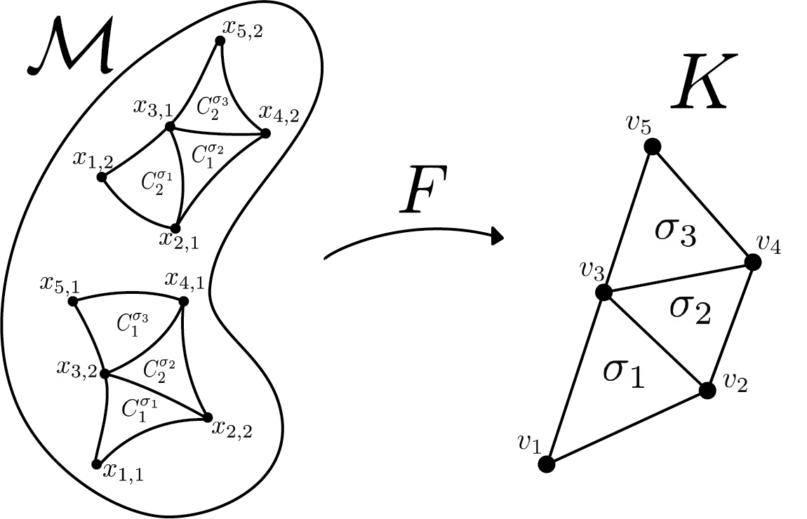
Figure 2: A sketch of the various quantities used in the proof of Theorem 2. This toy example provides a visual for the proof when $n=2$ and $d=2$. The blob on the left is $\mathcal{M}$, and the simplices on the right are a subset of $K$. As indicated by the hashing, $F(C^{\sigma_{1}}_{1})=F(C^{\sigma_{1}}_{2})=\sigma_{1}$, and likewise $F(C^{\sigma_{2}}_{1})=F(C^{\sigma_{2}}_{2})=\sigma_{2}$ and $F(C^{\sigma_{3}}_{1})=F(C^{\sigma_{3}}_{2})=\sigma_{3}$. Further, we have for each $i=1,\dots,5$ that $F(x_{i,1})=F(x_{k,2})=v_{1}$.

Proof.

The proof is quite involved and so we first provide a proof sketch highlighting the major steps of each section in the proof.

First, we show that for each $\sigma\in K$, there are $d$ disjoint compact patches $\left\{C^{\sigma}_{j}\right\}_{j=1}^{d}$ in $\mathcal{M}$ such that ${\left.\kern-1.2ptF\vphantom{\big{|}}\right|_{C^{\sigma}_{j}}}\colon C^{\sigma}_{j}\to\left\lvert\sigma\right\rvert$ is a homeomorphism for each $j$. A sketch of the patches $C^{\sigma}_{j}$ are shown in Figure 2.

Second, we construct a map $g^{\sigma}\colon\cup_{j=1}^{d}C^{\sigma}_{j}\to\left\lvert\sigma\right\rvert\times[0,d]$ where $g^{\sigma}(x)=\left(F(x),\cdot\right)$ that makes a $d$-tall ‘stack of pancakes’ over $\sigma$. Each of the $d$ pancakes is $F(C^{\sigma}_{j})$ for some $j$. We construct $g$ so that each pancake passes through $(v,i)$ for some $i\in 1,\dots,d$. We then construct a continuous map $g\colon\mathcal{M}\to\left\lvert K\right\rvert\times[0,d]$ so that ${\left.\kern-1.2ptg\vphantom{\big{|}}\right|_{\sigma}}=g^{\sigma}$.

Third we show that $g$ is a bijection between $\mathcal{M}_{1}$ and $\left\{(v,i)\right\}_{i=1}^{d}$, and that $g$ can be continuously lifted to an injective $h\colon\mathcal{M}\to C$ so that $h(x)=(g(x),\bm{0})$. Thus $h$ is a continuous and injective map between compact sets, and so is an embedding of $\mathcal{M}$ into $C$. Finally, we show that $p^{-1}(v)\cap h(\mathcal{M})=\left\{(v,i,\bm{0})\right\}_{i=1}^{d}$ for $\bm{0}\in\mathbb{R}^{2n}$. –

Let the vertices of $V$ be enumerated as $V=\left\{v_{1},\dots,v_{N}\right\}$ for some $N$, and for any $i\leq N$, let the set $X=\left\{x_{i,j}\right\}_{i=1,j=1}^{i=N,j=d}\subset\mathcal{M}$ be the $d$ points in $\mathcal{M}$ such that $F(x_{i,j})=v_{i}$.

1. Let $\sigma\in K$ be given, and $\left\{v_{1},\dots,v_{n+1}\right\}=\sigma\subset K$.

   We will construct one $C^{\sigma}_{j}$ for each $x_{1,j}$. Let $j$ be given, then defined $r_{j}=\min_{x\in F^{-1}(v_{1}),x\neq x_{1,j}}\lVert x-x_{1,j}\rVert$. Note that $r_{j}>0$, and $x_{1,j}=B_{r_{j}}(x_{1,j})\cap F^{-1}(v_{1})$. Let

   $$C^{\sigma}_{j}=B_{r_{j}}(x_{1,j})\cap F^{-1}(\left\lvert\sigma\right\rvert).$$

   We will show that ${\left.\kern-1.2ptF\vphantom{\big{|}}\right|_{C^{\sigma}_{j}}}$ is a homeomorphism.

   It is clear that ${\left.\kern-1.2ptF\vphantom{\big{|}}\right|_{C^{\sigma}_{j}}}$ is a local homeomorphism. Further, if $\sigma$ is small enough, then there is some $r^{\prime}<r_{j}$ so that $\left\lvert\sigma\right\rvert\subset F(B_{r^{\prime}}(x_{1,j}))$. Therefore, we have that ${\left.\kern-1.2ptF\vphantom{\big{|}}\right|_{C^{\sigma}_{j}}}\colon C^{\sigma}_{j}\to\left\lvert\sigma\right\rvert$. This is guaranteed from the assumption that the diameter of the largest $\sigma\in S$ is sufficiently small. From Lemma 5, we then have that ${\left.\kern-1.2ptF\vphantom{\big{|}}\right|_{C^{\sigma}_{j}}}$ is a covering map. Because $x_{1,j}=B_{r_{j}}(x_{1,j})\cap F^{-1}(v_{1})$, we can conclude that this covering map has degree one, and so ${\left.\kern-1.2ptF\vphantom{\big{|}}\right|_{C^{\sigma}_{j}}}$ is not just a local homeomorphism, but a proper homeomorphism. As an immediate consequence of this, we have that $C^{\sigma}_{j}$ is compact and connected.

2. 

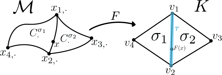
   Figure 3: Sketch of a toy example where a point $x$ is mapped to a simplex $\tau$ that is a common face of the simplices $\sigma_{1}$ and $\sigma_{2}$.

   From the previous part we have that for a choice of $\sigma$ and $j$, that $C^{\sigma}_{j}$ is compact and ${\left.\kern-1.2ptF\vphantom{\big{|}}\right|_{C^{\sigma}_{j}}}$ a homeomorphism. We also get that $C^{\sigma}_{j}$ are pairwise disjoint.

   Let us define the set of closed patches $\mathcal{C}=\left\{C^{\sigma}_{j}\colon\sigma\in S^{\max{}},j\in\left\{1,\dots,d\right\}\right\}$ where $S^{\max}\subset S$ are the maximal simplices of $S$. Now we introduce two index functions, $\operatorname{Ind}^{S}\colon\mathcal{C}\to\left\{1,\dots,d\right\}$ and $\operatorname{Ind}^{X}\colon X\to\left\{1,\dots,d\right\}$. They are defined as:

   $$\operatorname{Ind}^{S}(C) =j\text{ where }C=C^{\sigma}_{j}\in\mathcal{C}$$ (9)

   $$\operatorname{Ind}^{X}(x) =j\text{ where }x=x_{i,j}\in X.$$ (10)

   We note that the choices of $\operatorname{Ind}^{S}$ and $\operatorname{Ind}^{X}$ are not unique. The $j$ index in the definition of $\mathcal{C}$ and $X$ are both dummy indices. The key fact is that $C\mapsto(F(C),\operatorname{Ind}^{S}(C))$ and $x\mapsto(F(x),\operatorname{Ind}^{X}(x))$ are bijections.

   Let $y\in\left\lvert\sigma\right\rvert$. We can express $y$ in barycentric coordinates in terms of the vertices of $\sigma$. Let $\left(\lambda_{v}^{\sigma}(x)\right)_{v\in\sigma}$ be the unique scalars such that $F(x)=\sum_{v\in\sigma}\lambda_{v}^{\sigma}(x)v$, $\sum_{v\in\sigma}\lambda_{v}^{\sigma}(x)=1$ and $\lambda_{v}^{\sigma}(x)\geq 0$. Now define the function $g^{\sigma}_{k}\colon C^{\sigma}_{k}\to\left\lvert\sigma\right\rvert\times[0,d]$ as

   $$g^{\sigma}_{k}(x)=\left(F(x),\sum_{v\in\sigma}\operatorname{Ind}^{X}\left(F^{-1}(v)\cap C^{\sigma}_{k}\right)\lambda_{v}^{\sigma}(F(x))\right)$$ (11)

   Let us briefly prove some properties about $g^{\sigma}_{k}$. First, recall from part (a) that $F^{-1}(v)\cap C^{\sigma}_{k}\in X$, hence the $\operatorname{Ind}^{X}\left(F^{-1}(v)\cap C^{\sigma}_{k}\right)$ term is well-defined. Now we define

   $$g^{\sigma}\colon\bigcup^{d}_{k=1}C^{\sigma}_{k}\to\left\lvert\sigma\right\rvert\times[0,1],\quad g^{\sigma}(x)=g^{\sigma}_{\operatorname{Ind}^{S}(C)}(x)\text{ where }x\in C\in\mathcal{C}$$ (12)

   $$g\colon\mathcal{M}\to\left\lvert K\right\rvert\times[0,1],\quad g^{\sigma}(x)=\begin{cases}g^{\sigma_{1}}(x)&\text{if }F(x)\in\sigma_{1}\\ \vdots&\\ g^{\sigma_{N}}(x)&\text{if }F(x)\in\sigma_{N}\end{cases}$$ (13)

   Note that from part (a), we have that $\left\{C^{\sigma}_{k}\right\}_{k=1,\dots,d}$ are pairwise disjoint for any $\sigma$. Thus for any $x$, there is a unique $C\in\mathcal{C}$ so that $x\in C$. This shows that Equation 12 is well-defined. Equation 13, on the other hand, may have problems. In particular, it is possible for $F(x)\in\sigma$ and $F(x)\in\sigma^{\prime}$ for $\sigma\neq\sigma^{\prime}$. We resolve this problem by showing that if $F(x)\in\sigma\cap\sigma^{\prime}$, then $g^{\sigma}(x)=g^{\sigma^{\prime}}(x)$. This resolves the problem.

   Let $x\in\mathcal{M}$ be such that $F(x)\in\sigma\cap\sigma^{\prime}=\tau$, see Figure 3 for an illustration. Because $F(x)$ lies in the convex hull of $\tau$, we can then conclude that

   $$\lambda^{\sigma}_{v}(x)=\begin{cases}\lambda^{\tau}_{v}(x)&\text{if }v\in\tau\\ 0&\text{if }v\not\in\tau\end{cases}.$$ (14)

   and likewise for $\sigma^{\prime}$. Expanding the definition of $g^{\sigma}(x)$ we get that there is some $k$ so that

   $$g^{\sigma}(x) =\left(F(x),\sum_{v\in\sigma}\operatorname{Ind}^{X}\left(F^{-1}(v)\cap C^{\sigma}_{k}\right)\lambda_{v}^{\sigma}(F(x))\right)$$ (15)

   $$=\left(F(x),\sum_{v\in\tau}\operatorname{Ind}^{X}\left(F^{-1}(v)\cap C^{\sigma}_{k}\right)\lambda_{v}^{\sigma}(F(x))+\sum_{v\in\sigma\setminus\tau}\operatorname{Ind}^{X}\left(F^{-1}(v)\cap C^{\sigma}_{k}\right)\lambda_{v}^{\sigma}(F(x))\right)$$ (16)

   $$=\left(F(x),\sum_{v\in\tau}\operatorname{Ind}^{X}\left(F^{-1}(v)\cap C^{\sigma}_{k}\right)\lambda_{v}^{\tau}(F(x))\right).$$ (17)

   Likewise, $g^{\sigma^{\prime}}(x)=\left(F(x),\sum_{v\in\tau}\operatorname{Ind}^{X}\left(F^{-1}(v)\cap C^{\sigma^{\prime}}_{k^{\prime}}\right)\lambda_{v}^{\tau}(F(x))\right)$ for some $k^{\prime}$. Finally, we have that $F^{-1}(\left\lvert\tau\right\rvert)\cap C^{\sigma}_{k}=F^{-1}(\left\lvert\tau\right\rvert)\cap C^{\sigma^{\prime}}_{k^{\prime}}$. Thus we have $F^{-1}(v)\cap C^{\sigma}_{k}=F^{-1}(v)\cap C^{\sigma^{\prime}}_{k^{\prime}}$. This proves that $g^{\sigma}(x)=g^{\sigma^{\prime}}(x)$.

   Clearly, $g$ is continuous on the interior of every maximal simplex $\sigma\in S^{\max}$. The previous result shows that $g$ is continuous across the boundry of all simplices. Therefore, we also obtain continuity of $g$ by the gluing lemma.

3. Before we construct $h$, we will show that ${\left.\kern-1.2ptg\vphantom{\big{|}}\right|_{X}}$ is a bijection from $X$ onto $\left\{(v,i)\right\}_{i=1,\dots,d}$. Let $x\in X$, then $F(x)=v^{\prime}\in\sigma$ for some $\sigma\in S^{\max}$, and for that choice of $\sigma$, there is a unique $k$ so that $x\in C^{\sigma}_{k}$. Uniqueness follows from separation of $C^{\sigma}_{k}$. Hence

   $$g(x)=g^{\sigma}(x)=g^{\sigma}_{k}(x).$$

   Evaluating the value of $g^{\sigma}_{k}$ and using the identity

   $$\lambda^{\sigma}_{v^{\prime}}(v)=\begin{cases}1&\text{if }v^{\prime}=v\\ 0&\text{if }v^{\prime}\neq v\end{cases}$$ (18)

   we obtain

   $$g(x)=g^{\sigma}_{k}(x) =\left(v^{\prime},\sum_{v\in\sigma}\operatorname{Ind}^{X}\left(F^{-1}(v)\cap C^{\sigma}_{k}\right)\lambda_{v}^{\sigma}(v^{\prime})\right)$$ (19)

   $$=\left(v^{\prime},\operatorname{Ind}^{X}(x)\lambda_{v^{\prime}}(v^{\prime})+\sum_{v\in\sigma,v\ \neq v^{\prime}}\operatorname{Ind}^{X}\left(F^{-1}(v)\cap C^{\sigma}_{k}\right)\underbrace{\lambda_{v}^{\sigma}(v^{\prime})}_{=0\text{ as }v\neq v^{\prime}}\right)$$ (20)

   $$=\left(v^{\prime},\operatorname{Ind}^{X}(x)\right).$$ (21)

   If $x_{i,j}$ and $x_{i^{\prime},j^{\prime}}$ are such that $g(x_{i,j})=g(x_{i^{\prime},j^{\prime}})$, then equality in the $v$ component of Eqn. 21 proves that $i=i^{\prime}$ and equality in the $\operatorname{Ind}^{X}$ component of Eqn. 21 proves that $j=j^{\prime}$. This proves that $g$ is injective on $X$. Both $X$ and $\left\{(v,i)\right\}_{v\in V,i=1,\dots,d}$ have $\#(V)=d$ elements, therefore bijectivity follows from injectivity.

   Now we turn to showing that $g$ can be continuously lifted to a function $h\colon\mathcal{M}\to C$ that is injective on all of $\mathcal{M}$, and so an embedding. Before starting with that proof, we remark on the non-injectivity of $g$. Because $g_{k}^{\sigma}$ is a homeomorphism, ${\left.\kern-1.2ptg\vphantom{\big{|}}\right|_{C^{\sigma}_{k}}}$ is injective and so $g$ is locally injective, but $g$ may fail to be injective globally. Consider for example the case when $R^{\sigma}(v_{1},1)=1,R^{\sigma}(v_{2},1)=2,R^{\sigma}(v_{1},2)=2,R^{\sigma}(v_{2},2)=1$, $\tilde{x}_{1}\in C^{\sigma}_{1}$ and $\tilde{x}_{2}\in C^{\sigma}_{2}$ be such that $F(\tilde{x}_{1})=F(\tilde{x}_{2})=\frac{1}{2}\left(v_{1}+v_{2}\right)$, then

   $$g(\tilde{x}_{1})=\left(\frac{1}{2}\left(v_{1}+v_{2}\right),1\frac{1}{2}+2\frac{1}{2}\right)=\left(\frac{1}{2}\left(v_{1}+v_{2}\right),2\frac{1}{2}+1\frac{1}{2}\right)=g(\tilde{x}_{2})$$

   If there is a $\sigma\in S$ and indices $1\leq k_{1},k_{2}\leq d$ and vertices $v,v^{\prime}\in V$ such that $R^{\sigma}(v,k_{1})<R^{\sigma}(v,k_{2})$ and $R^{\sigma}(v^{\prime},k_{1})<R^{\sigma}(v^{\prime},k_{2})$ then $g$ is non-injective. This follows from Equation 21 and the intermediate value theorem. Indeed if $\mathcal{M}$ is connected then $g(\mathcal{M})$ always has self intersections. If not, otherwise the maximal (in the final coordinate) components of $g(\mathcal{M})$ would be both open and closed, which violates connectedness of $\mathcal{M}$.

   Now we construct the embedding $h$. From Whitney’s embedding theorem and compactness there is an embedding of $\mathcal{M}$ into $[0,1]^{2n}$. Let $f:\mathcal{M}\to[0,1]^{2n}$ be that embedding, Further let $\epsilon>0$ be such that ${\left.\kern-1.2ptg\vphantom{\big{|}}\right|_{\cup_{x\in X}B_{\epsilon}(x)}}$ is injective. The existence of such an $\epsilon$ follows from continuity of $g$ and that ${\left.\kern-1.2ptg\vphantom{\big{|}}\right|_{X}}$ is injective. Let $\psi_{x,\epsilon}\colon\mathcal{M}\to\mathbb{R}$ be a bump function such that $\psi(x)=1$, $\psi$ is smooth, and $\psi=0$ outside of $B_{\epsilon}(x)$. Then we define

   $$\Psi(y) =\sum_{x\in X}\psi_{x,\epsilon}(y)$$ (22)

   $$h(y) =\left(g(y),\Psi(y)f(y)\right).$$ (23)

   Let $\pi_{1}\colon\mathbb{R}^{n+1}\times\mathbb{R}^{2n}\to\mathbb{R}^{n+1}$ and $\pi_{2}\colon\mathbb{R}^{n+1}\times\mathbb{R}^{2n}\to\mathbb{R}^{2n}$ be coordinate projections. On $\cup_{x\in X}B_{\epsilon}(x)$, $\pi_{1}\circ h=g$ is injective owning to $g$’s injectivity. On $\mathcal{M}\setminus\cup_{x\in X}B_{\epsilon}(x)$, $\pi_{2}\circ h=f$ and so is injective as well. Clearly $h$ is continuous. $h$ is a continuous injection on a compact set and so is an embedding. This concludes part 3, and the entire proof overall.

∎

B.9 Proof of Theorem 3

Before we prove Theorem 3, we first prove a helper lemma. This lemma shows that given a triangulation $K$ we can always find a finer triangulation $K^{\prime}$ with vertices at an arbitrary set of points $Y\subset\left\lvert K^{\prime}\right\rvert$.

Lemma 6 (Vertexed Triangulations).

Let $K$ be a $n$ triangulation, and $Y\subset\left\lvert K\right\rvert$ a finite set of points. Then there is a triangulation $K^{\prime}=(V^{\prime},S^{\prime})$ of $K$ so that $Y\subset V^{\prime}$.

Proof.

We proceed by induction on the size of $Y$. The base case when $Y=\emptyset$ is solved by letting $K^{\prime}=K$. Now the inductive step. Let $y\in Y$, so that $Y=\left\{y\right\}\cup\left(Y\setminus\left\{y\right\}\right)$. If $y$ is already a vertex of $K^{\prime}$ then we are done. Otherwise, there is some $\sigma\in S$ so that $y\in\sigma^{o}$ where $\sigma^{o}$ denotes the relative interior of $\sigma$. Then, we can subdivide (like a barycentric subdivision but at $y$ instead of the barycenter) $\sigma$ at $y$ into $n+1$ simplices. Call these simplices $\Sigma_{y}$. We form a triangulation $K^{\prime}$ by removing $\sigma$ and replacing it with this subdivision. For each coface $\tau\in S$ of $\sigma$, replace $\sigma$ in $\tau$ with one element each of $\Sigma_{y}$. A long but straight forward calculation shows that after this coface replacement is legitimate, this yields a simplicial complex $\tilde{K}$ with vertex at $y$. Now apply the inductive hypothesis to $\tilde{K}$ and the points $Y\setminus\left\{y\right\}$. ∎

Now we prove Theorem 3.

Proof.

The manifold $\mathcal{M}_{2}$ is smooth, and so triangulable. Let $K_{2}=(V_{2},S_{2})$ be a triangulation of $\mathcal{M}_{2}$ with diffeomorphism $h_{2}\colon K_{2}\to\mathcal{M}_{2}$.

We apply Lemma 6 to the triangulation $K_{2}=(V_{2},S_{2})$ where the set of points that we want to add to the vertex of the triangulation is $h^{-1}_{2}(Y)$. Note that $Y$ is finite, and $Y\subset\mathcal{M}_{2}$, and so $h^{-1}_{2}(Y)\subset\left\lvert K_{2}\right\rvert$, and so the lemma applies. Thus, there is a triangulation $K^{\prime}=(V^{\prime},S^{\prime})$ of $\mathcal{M}_{2}$ with vertices that include $h^{-1}_{2}(Y)$. Now we apply Theorem 2, and obtain projection $p\colon C\to\left\lvert K_{2}\right\rvert$ and $h\in\operatorname*{emb}^{1}(\mathcal{M}_{1},C)$ so that for $C=\left\lvert K_{2}\right\rvert\times[0,d]\times[0,1]^{n}$ we have that $h_{2}^{-1}\circ g=p\circ h$. Moreover, we have that for each $y\in h^{-1}_{2}(Y)\subset V^{\prime}$, $p^{-1}(v)\cap h(\mathcal{M}_{1})=\left\{(v,i,\bm{0})\right\}$ for $i=1,\dots,d$.

Applying $h_{2}$ to both sides, we get that $g=h_{2}\circ p\circ h$, and for every $y\in Y$

$$g^{-1}(y)=h^{-1}\circ p^{-1}\circ h^{-1}_{2}(y)=h^{-1}\left(\left\{v,i,\bm{0}\right\}_{i=1,\dots,d}\right)$$

where $v=h_{2}^{-1}(y)$.

To form the sequence of $f_{i}$ and $X_{i}$ that satisfy Eqn.s 4 and 5, choose a sequence $\left(E{}_{1}\right)^{\infty}_{1=i}$ and $\left(T{}_{1}\right)^{\infty}_{1=i}$ so that $E_{i}$ and $T_{i}$ are, respectively, bistable uniform approximators to the embedding $h$ and diffeomorphism $h_{2}$. If we define $f_{i}\coloneqq T_{i}\circ p\circ E_{i}$ then by compactness $\left(f{}_{1}\right)^{\infty}_{1=i}$ is a bistable uniform approximator. for $g$. Further, by inverse Lipschitz-ness of $g$ and $f_{i}$, we have for all $y\in Y$ that

$$\sup_{y\in Y}\lVert h^{-1}\circ\left(h^{-1}_{2}(y),i,\bm{0}\right)-E_{i}^{-1}\left(T_{i}^{-1}(y),i,\bm{0}\right)_{\mathbb{R}^{m_{1}}}\rVert\leq\epsilon_{i}$$ (24)

where $\epsilon_{i}\to 0$ as $i\to\infty$. This proves Eqn. 5. ∎

B.10 Proof of Corollary 4

In this subsection we present the proof of Corollary 4.

Proof.

The proof of this follows from $\overline{\operatorname*{emb}^{1}(\mathcal{M}_{1},\mathbb{R}^{m_{2}})}\subset\operatorname{lochom}(\mathcal{M}_{1},\mathcal{M}_{2})$. If $\left(f{}_{n}\right)^{\infty}_{n=1}$ was a uniform approximating sequence for $g$, then $g$ would necessarily be a local homeomorphism between $\mathcal{M}_{1}$ and $\mathcal{M}_{2}$. This is a contradiction, hence no such sequence exists. ∎

B.11 Proof of Lemma 2

In this section we present the proof of Lemma 2

Proof.

First, we prove that $\mathcal{M}_{1}/\Sigma$ is a manifold. Because $\Sigma$ is finite, $\pi_{\Sigma}$ is a proper and continuous. It is free because orbits are all the same size, hence $\mathcal{M}_{1}/\Sigma$ is a manifold from [53, Theorem 21.10].

1. ${\left.\kern-1.2ptf\vphantom{\big{|}}\right|_{\mathcal{M}_{1}/\Sigma}}$ is the unique map satisfying Eqn. 6. This is shown by passing to the quotient as in [53, Theorem A.30].

2. Clearly $\pi_{\Sigma}$ is a covering space of $\mathcal{M}_{1}/\Sigma$ by $\mathcal{M}_{2}$. From $f$ and $\pi_{\Sigma}$ being $d$-to-one we obtain that $f$ is one-to-one, and so it is a diffeomorphism, so $f_{\mathcal{M}_{1}/\Sigma}\circ\pi_{\Sigma}$ is a smooth covering map, and so is a local diffeomorphism

∎

B.12 Proof of Corollary 5

In this section we present the proof of Corollary 5.

Proof.

This follows from Eqn. 5. By uniform inverse lipschitzness of $E_{i}$, we have that $X_{i}$ converges $f_{i}^{-1}(Y)$, and so Eqn. 5 becomes that $d_{H}(f_{i}^{-1}(Y),g^{-1}(Y))\to 0$. From inverse Lipschitz-ness of $g$ and $f$ we have that, for $i$ large enough, that $f_{i}^{-1}(Y)$ and $g^{-1}(Y)$ have the same number of points, hence $d_{H}(f_{i}^{-1}(y),g^{-1}(y))$ for each $y\in Y$. ∎

B.13 Proof of Lemma 3

In this section we present the proof of Lemma 3.

Proof.

Let $m=k\left(n-1\right)+1$, where $n,m$ and $k$ are positive integers, $k\geq 2$. In this section we explicitly construct a covering of a genus $n$ surface $S_{n}$ with a genus $m$ surface $S_{m}$. We consider coordinates $(x,y,s,z,t)$ in $\mathbb{R}^{5}$. Let $P_{4}:\mathbb{R}^{5}\to\mathbb{R}^{4},P_{2}:\mathbb{R}^{5}\to\mathbb{R}^{3},P_{2}:\mathbb{R}^{5}\to\mathbb{R}^{2},Q_{4}:\mathbb{R}^{5}\to\mathbb{R}^{3},R_{2}:\mathbb{R}^{4}\to\mathbb{R}^{2}$ be the projections where

$$P_{2}(x,y,s,z,t) =(x,y)$$

$$P_{3}(x,y,s,z,t) =(x,y,s)$$

$$P_{4}(x,y,s,z,t) =(x,y,s,z)$$

$$Q_{3}(x,y,s,z,t) =(x,y,z)$$

$$Q_{4}(x,y,s,z,t) =(x,y,z,t)$$

$$R_{2}(x,y,z,t) =(x,y).$$

Consider curve $\gamma:[-2(k-1)\pi,2(k-1)\pi]\to\mathbb{R}^{5}$ given by

$$\gamma(r)=(\cos(r),\sin(r),0,\phi(r),\psi(r))$$ (25)

where $\phi,\psi\in C^{\infty}(\mathbb{R})$ are such that

$$\psi(r)\geq 0,\quad\text{ for all $r$, and}$$

$$\psi(r)>0,\quad\text{ if and only if $|r-(-2j+1)\pi|<1$ for some $j=1,2,\dots,k-1$}$$

and

$$\phi(-r)=\phi(r,)$$

$$\phi(r)=1,\quad\text{for $r\in[0,\pi/2]$,}$$

$$\phi(r)=j+1,\quad\text{for $r\in[(2j-\frac{1}{2})\pi,(2j+\frac{1}{2})\pi]$, $j=1,2,3,\dots,k-2$},$$

$$\phi(r)=k,\quad\text{for $r\in[((k-1)-\frac{1}{2})\pi,2(k-1)\pi]$},$$

$$\phi((2j-1)\pi)=j-\frac{1}{2},\quad j=1,2,\dots,k-1$$

$$r\to\phi(r),\quad\text{is strictly increasing on the intervals $r\in[(2j+\frac{1}{2})\pi,(2j+\frac{3}{2})\pi]$, $j=0,1,2,\dots,k-2$}.$$

Then

$$P_{4}(\gamma(-r))=P_{4}(\gamma(-s))\hbox{ if and only if $r=s=j\pi$ for some $j=1,2,\dots,k-1$}.$$ (26)

and $\gamma([-2(k-1)\pi,2(k-1)\pi])$ is a smooth closed curve in $\mathbb{R}^{5}$ which does not intersect itself.

Let $\mu(r)=Q_{4}(\gamma(r))$ be a smooth curve in $\mathbb{R}^{4}$ that has no self-intersections. Then $\alpha(r)=R_{2}(\mu(r))$ is such that the set $\alpha([0,2\pi])=\alpha([-2(k-1)\pi,2(k-1)\pi])\subset\mathbb{R}^{2}$ is the unit circle in $\mathbb{R}^{2}$ and the projection

$$R_{2}:\mu([-2(k-1)\pi,2(k-1)\pi])\to\alpha([0,2\pi])$$ (27)

is a $k$-to-1 covering map.

We will first consider a 2-dimensional torus $\Sigma_{0}$ in $\mathbb{R}^{5}$ whose “central curve” is the path $\gamma$. In other words, a tube with central axis $\gamma$. To this end, let

$$v(r)=\frac{1}{|\partial_{r}P_{2}(\gamma(r))|}\partial_{r}P_{2}(\gamma(r))$$ (28)

be the unit tangent vector of the curve $r\to P_{2}(\gamma(r))$ in $\mathbb{R}^{2}$ and let

$$\nu(r)=v(r)^{\perp}$$ (29)

be the unit normal vector of the curve $r\to P_{2}(\gamma(r))$ in $\mathbb{R}^{2}$ which is obtained by rotating $v(r)$ $90\degree$ clockwise in $\mathbb{R}^{2}$. Let

$$\tilde{\nu}(r)=(\nu(r),0,0,0)$$ (30)

be a vector in $\mathbb{R}^{5}$ and $\hat{e}=(0,0,1,0,0)$ be a unit vector in $\mathbb{R}^{5}$ pointing to the direction of the $s$-axis.

Let $H:[-2(k-1)\pi,2(k-1)\pi]\times[-\pi,\pi]\to\mathbb{R}^{5}$ be the function

$$H(r,\theta)=\gamma(r)+\cos(\theta)\nu(r)+\sin(\theta)\hat{e}.$$ (31)

We define

$$\Sigma_{0}=H([-2(k-1)\pi,2(k-1)\pi]\times[-\pi,\pi])$$ (32)

to be a 2-dimensional surface in $\mathbb{R}^{5}$. The surface $\Sigma_{0}$ is a 2-dimensional torus in $\mathbb{R}^{5}$. It has the property that the surface $\Sigma_{1}=P_{3}(\Sigma_{0})$ is a 2-dimensional torus in $\mathbb{R}^{3}$ and the projection

$$P_{3}:\Sigma_{0}\to\Sigma_{1}$$ (33)

is a 2-to-1 covering map. Observe that the points $q_{j}=H(2j\pi,0)=(1,0,0,j+1,0)$, $j=0,1,2,\dots,k-1$ have neighborhoods $U_{j}$ in $\mathbb{R}^{5}$ such that $\Sigma_{0}\cap U_{j}$ is a subset of $\mathbb{R}^{3}\times\{(j,0)\}$ and the maps

$$\rho_{i,j}:(x,y,s,z,t)\to(x,y,s,z+(j-i),t),\quad i,j\in\{0,1,2,\dots,k-1\},\ i<j$$ (34)

are bijections

$$\rho:\Sigma_{0}\cap U_{i}\to\Sigma_{0}\cap U_{j}.$$ (35)

Now, we add $n$ handlebodies to $\Sigma_{0}$. We modify $\Sigma_{0}$ in the sets $U_{j}$ by smoothly gluing to $\Sigma_{0}\cap U_{j}$ a collection of $(n-1)$ 2-dimensional toruses $T_{j,p}\subset U_{j}\cap\mathbb{R}^{3}\times\{(j,0)\}$, $p=1,2,\dots,n-1$ so that we obtain a $C^{\infty}$-smooth surface

$$S_{m}=\Sigma_{0}\#(T_{1,1}\#T_{1,2}\#\dots\#T_{1,n-1})\#(T_{2,1}\#T_{2,2}\#\dots\#T_{2,n-1})\#\dots\#(T_{j,1}\#T_{j,2}\#\dots\#T_{j,n-1})$$ (36)

that has genus $m=k\left(n-1\right)+1$ and moreover, $S_{m}\cap U_{i}\subset\mathbb{R}^{3}\times\{(i+1,0)\}$ and the maps

$$\rho_{i,j}:S_{m}\cap U_{i}\to S_{m}\cap U_{j}$$ (37)

are bijection for all $i<j$. Then $S_{n}=P_{3}(S_{m})$ is a smooth surface in $\mathbb{R}^{3}$ that has genus $n$ and the projection

$$P_{3}:S_{m}\to S_{n}$$ (38)

is a $k$-to-1 covering map. This show that in $\mathbb{R}^{5}$ there is a surface $S_{m}$ with genus $m$ that is mapped in the projection $P_{3}$ to a surface $S_{n}$ in $\mathbb{R}^{3}$ with genus $n$ ,and for these surfaces $P_{3}$ is a $k$-to-1 covering map.

∎

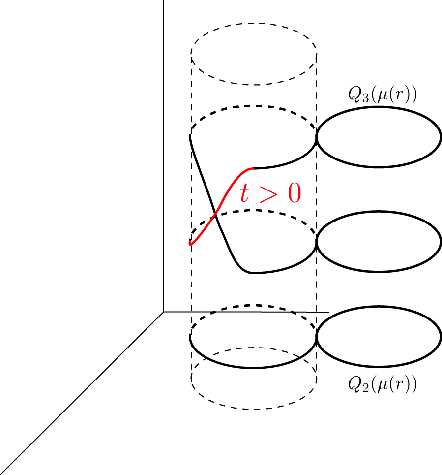
Figure 4: Explanation of the proof of Lemma 3 in the case when $m=3$, $n=2$ and $k=2$. Curve $Q_{3}(\mu(r))$ in $\mathbb{R}^{3}$. In fact, the figure can be considered also as a 4-dimensional curve $Q_{4}(\mu(r))$ when the red colour shows where $t>0$ and the black colour where $t=0$. Note that projection $R_{2}:Q_{4}(\mu([-2\pi,2\pi]))\to Q_{2}(\mu([-2\pi,2\pi]))$ is 2-to-1 covering map. With dotted lines in the figure we have also indicated the projected core curves of the toruses which we glue to $\Sigma_{0}$ to obtain a surface $S_{3}$ and the projected core curve of the torus that is glued in $\Sigma_{1}$ to obtain a surface $S_{2}$.

B.14 Proof of Theorem 4

Proof.

We can assume without loss of generality that ${\tilde{m}_{1}}\geq 3m_{1}+1$. Otherwise, we may replace $\tilde{\mathcal{M}}_{1}$ by $J_{0}(\tilde{\mathcal{M}}_{1})$ where $J_{0}\colon\mathbb{R}^{\tilde{m}_{1}}\to\mathbb{R}^{3m_{1}}$ where $J_{0}(x)\coloneqq(x,\left\{0\right\}^{3m_{1}+1-\tilde{m}_{1}})$.

Let us now return to proof assuming that ${\tilde{m}_{1}}\geq 3m_{1}+1$. Let $J_{1}\colon\mathbb{R}^{m_{1}}\to\mathbb{R}^{m_{1}}\times\{0\}^{\tilde{m}_{1}-{m_{1}}}\subset\mathbb{R}^{\tilde{m}_{1}}$ be the linear injective map $J_{1}(x)\coloneqq(x,0)$. Then $J_{1}|_{\mathcal{M}_{1}}\colon\mathcal{M}_{1}\to\widehat{\mathcal{M}}_{1}\eqqcolon J_{1}(\mathcal{M}_{1})$ is a diffeomorphism. Also, let $E_{1}:\mathbb{R}^{m_{1}}\times\mathbb{R}^{\tilde{m}_{1}-{m_{1}}}\to\mathbb{R}^{m_{1}}$ be the projection to the first coordinate.

As $\mathcal{M}_{1}$ and $\tilde{\mathcal{M}}_{1}$ are diffeomorphic, there is a diffemorphism $g_{1}\colon\mathcal{M}_{1}\to\tilde{\mathcal{M}}_{1}$. Then, $\tilde{g}_{1}=g_{1}\circ E_{1}\colon\widehat{\mathcal{M}}_{1}\to\tilde{\mathcal{M}}_{1}$ is a diffeomorphism, too. We recall that $\mathcal{M}_{1}\subset\mathbb{R}^{m_{1}}$ and $\tilde{\mathcal{M}}_{1}\subset\mathbb{R}^{\tilde{m}_{1}}$. Then, as $\tilde{m}_{1}\geq 3m_{1}+1$, we can apply [56, Lemma 7.6] and [71, Thm. 3.8] to the embedding $g_{1}\colon\mathcal{M}_{1}\to\mathbb{R}^{\tilde{m}_{1}}$ and see that there is an injective linear map $L_{1}:\mathbb{R}^{m_{1}}\to\mathbb{R}^{\widetilde{m}_{1}}$ and a diffeomorphims $D_{1}:\mathbb{R}^{\widetilde{m}_{1}}\to\mathbb{R}^{\widetilde{m}_{1}}$ such that

$$g_{1}=D_{1}\circ L_{1}|_{\widehat{\mathcal{M}}_{1}},$$

that is, the embedding $g_{1}$ is an extendable embedding (see [71, Def. 3.7]. By basic results of linear algebra, there is a linear bijection $B_{1}:\mathbb{R}^{m_{1}}\times\mathbb{R}^{\widetilde{m}_{1}-{m_{1}}}=\mathbb{R}^{\widetilde{m}_{1}}\to\mathbb{R}^{\widetilde{m}_{1}}$ such that for $x\in\mathbb{R}^{m_{1}}$ we have $B_{1}(x,0)=L_{1}(x)$. This implies that $\tilde{g}_{1}:\tilde{\mathcal{M}}_{1}\to\mathbb{R}^{\widetilde{m}_{1}}$ extends to a diffeomorphism $T_{1}=D_{1}\circ B_{1}\colon\mathbb{R}^{\widetilde{m}_{1}}\to\mathbb{R}^{\widetilde{m}_{1}}$, so that $T_{1}|_{\widehat{\mathcal{M}}_{1}}=\tilde{g}_{1}$. Observe that $T_{1}\circ J_{3}|_{\mathcal{M}_{1}}=g_{3}$ is a diffeomorphims from $\mathcal{M}_{1}$ to $\tilde{\mathcal{M}}_{1}$. We recall that by assumption, the projection $p:\tilde{\mathcal{M}}_{2}\to\tilde{\mathcal{M}}_{1}$ is a covering map. Then the restriction of the map $p\circ T_{3}\circ J_{3}\colon\mathbb{R}^{m_{1}}\to\mathbb{R}^{\widetilde{m}_{2}}$ on ${\mathcal{M}_{1}}$, that we denote by $p\circ T_{3}\circ J_{3}|_{\mathcal{M}_{1}}\colon\mathcal{M}_{1}\to\tilde{\mathcal{M}}_{2}$, is a covering map.

Next, consider the submanifold $\mathcal{M}_{2}$ in $\mathbb{R}^{m_{2}}$. Let us use the map $E_{2}\colon\mathbb{R}^{m_{2}}\to\mathbb{R}^{{m_{2}}+\widetilde{k}}$ where $\widetilde{k}=m_{2}-k$, defined by $E_{2}(x)\coloneqq(x,0)$, to embed $\mathcal{M}_{2}$ into $\mathbb{R}^{{m_{2}}+\widetilde{k}}$ to the manifold $\widehat{\mathcal{M}}_{2}\coloneqq E_{2}(\mathcal{M}_{2})\subset\mathbb{R}^{\widetilde{k}}$. We then have that $p_{2}\colon\mathbb{R}^{{m_{2}}+\widetilde{k}}\to\mathbb{R}^{m_{2}}$, $p_{2}\colon(x,y)=x$ defines a diffeomorphism $p_{2}\colon\widehat{\mathcal{M}}_{2}\to\mathcal{M}_{2}$. We assume that $\widetilde{m}_{2}+\widetilde{k}\geq 3m_{2}+1$.

Similarly to the above, let $J_{2}\colon\mathbb{R}^{\widetilde{m}_{2}}\to\mathbb{R}^{\widetilde{m}_{2}}\times\{0\}^{\widetilde{k}-\widetilde{m}_{2}}\subset\mathbb{R}^{\widetilde{k}}$ be a linear injective map $J_{2}(x)\coloneqq(x,0)$. Then $J_{2}|_{\tilde{\mathcal{M}}_{2}}:\tilde{\mathcal{M}}_{2}\to\hat{\mathcal{M}}_{2}\eqqcolon J_{2}(\tilde{\mathcal{M}}_{1})$ is a diffeomorphism.

As there is a diffeomorphism $\tilde{g}_{2}\colon\tilde{\mathcal{M}}_{2}\to\widehat{\mathcal{M}}_{2}$ and $k\geq 3m_{2}+1$, we see as above by using [56, Lemma 7.6] and [71, Thm. 3.8] that $\tilde{g}_{2}$ extends to a diffeomorphism $T_{2}\colon\mathbb{R}^{k}\to\mathbb{R}^{k}$, so that $T_{2}|_{\tilde{\mathcal{M}}_{2}}=\tilde{g}_{2}$. Then we see that the map

$$p_{2}\circ T_{2}\circ J_{2}\circ p\circ T_{3}\circ J_{3}\bigg{|}_{\mathcal{M}_{1}}\colon\mathcal{M}_{1}\to\mathcal{M}_{2}$$

is a covering map. ∎

References

• [1] Giovanni S Alberti, Ángel Arroyo, and Matteo Santacesaria. Inverse problems on low-dimensional manifolds. arXiv preprint arXiv:2009.00574, 2020.
• [2] Tomás Angles and Stéphane Mallat. Generative networks as inverse problems with scattering transforms. arXiv preprint arXiv:1805.06621, 2018.
• [3] Rushil Anirudh, Jayaraman J Thiagarajan, Bhavya Kailkhura, and Timo Bremer. An unsupervised approach to solving inverse problems using generative adversarial networks. arXiv preprint arXiv:1805.07281, 2018.
• [4] Lynton Ardizzone, Jakob Kruse, Sebastian Wirkert, Daniel Rahner, Eric W Pellegrini, Ralf S Klessen, Lena Maier-Hein, Carsten Rother, and Ullrich Köthe. Analyzing inverse problems with invertible neural networks. arXiv preprint arXiv:1808.04730, 2018.
• [5] Jens Behrmann, Will Grathwohl, Ricky TQ Chen, David Duvenaud, and Jörn-Henrik Jacobsen. Invertible residual networks. arXiv preprint arXiv:1811.00995, 2018.
• [6] Mikhail Belkin and Partha Niyogi. Semi-supervised learning on riemannian manifolds. Machine learning, 56(1):209–239, 2004.
• [7] Mikhail Belkin, Partha Niyogi, and Vikas Sindhwani. Manifold regularization: A geometric framework for learning from labeled and unlabeled examples. Journal of machine learning research, 7(11), 2006.
• [8] Tamir Bendory, Alberto Bartesaghi, and Amit Singer. Single-particle cryo-electron microscopy: Mathematical theory, computational challenges, and opportunities. IEEE signal processing magazine, 37(2):58–76, 2020.
• [9] Mira Bernstein, Vin De Silva, John C Langford, and Joshua B Tenenbaum. Graph approximations to geodesics on embedded manifolds. Technical report, Citeseer, 2000.
• [10] Alberto Bietti, Luca Venturi, and Joan Bruna. On the sample complexity of learning under geometric stability. Advances in Neural Information Processing Systems, 34:18673–18684, 2021.
• [11] Jeremiah Birrell, Markos A Katsoulakis, Luc Rey-Bellet, and Wei Zhu. Structure-preserving gans. arXiv preprint arXiv:2202.01129, 2022.
• [12] Johann Brehmer and Kyle Cranmer. Flows for simultaneous manifold learning and density estimation. Advances in Neural Information Processing Systems, 33:442–453, 2020.
• [13] Michael M Bronstein, Joan Bruna, Taco Cohen, and Petar Veličković. Geometric deep learning: Grids, groups, graphs, geodesics, and gauges. arXiv preprint arXiv:2104.13478, 2021.
• [14] Michael M Bronstein, Joan Bruna, Yann LeCun, Arthur Szlam, and Pierre Vandergheynst. Geometric deep learning: going beyond euclidean data. IEEE Signal Processing Magazine, 34(4):18–42, 2017.
• [15] Rickard Brüel-Gabrielsson, Bradley J Nelson, Anjan Dwaraknath, Primoz Skraba, Leonidas J Guibas, and Gunnar Carlsson. A topology layer for machine learning. arXiv preprint arXiv:1905.12200, 2019.
• [16] Gunnar Carlsson. Topology and data. Bulletin of the American Mathematical Society, 46(2):255–308, 2009.
• [17] Lawrence Cayton. Algorithms for manifold learning. Univ. of California at San Diego Tech. Rep, 12(1-17):1, 2005.
• [18] Anadi Chaman and Ivan Dokmanic. Truly shift-invariant convolutional neural networks. In Proceedings of the IEEE/CVF Conference on Computer Vision and Pattern Recognition, pages 3773–3783, 2021.
• [19] Rewon Child. Very deep vaes generalize autoregressive models and can outperform them on images. arXiv preprint arXiv:2011.10650, 2020.
• [20] Edmond Cunningham, Renos Zabounidis, Abhinav Agrawal, Ina Fiterau, and Daniel Sheldon. Normalizing flows across dimensions. arXiv preprint arXiv:2006.13070, 2020.
• [21] George Cybenko. Approximation by superpositions of a sigmoidal function. Mathematics of control, signals and systems, 2(4):303–314, 1989.
• [22] Bin Dai and David Wipf. Diagnosing and enhancing vae models. arXiv preprint arXiv:1903.05789, 2019.
• [23] Laurent Dinh, David Krueger, and Yoshua Bengio. Nice: Non-linear independent components estimation. arXiv preprint arXiv:1410.8516, 2014.
• [24] Laurent Dinh, Jascha Sohl-Dickstein, and Samy Bengio. Density estimation using real nvp. arXiv preprint arXiv:1605.08803, 2016.
• [25] Stefania Ebli, Michaël Defferrard, and Gard Spreemann. Simplicial neural networks. arXiv preprint arXiv:2010.03633, 2020.
• [26] Lawrence C Evans. Partial differential equations. Graduate studies in mathematics, 19(2), 1998.
• [27] Charles Fefferman, Sergei Ivanov, Yaroslav Kurylev, Matti Lassas, and Hariharan Narayanan. Reconstruction and interpolation of manifolds. I: The geometric Whitney problem. Found. Comput. Math., 20(5):1035–1133, 2020.
• [28] Charles Fefferman, Sanjoy Mitter, and Hariharan Narayanan. Testing the manifold hypothesis. Journal of the American Mathematical Society, 29(4):983–1049, 2016.
• [29] Joachim Frank. Electron tomography: methods for three-dimensional visualization of structures in the cell. Springer Science & Business Media, 2008.
• [30] Octavian Ganea, Gary Bécigneul, and Thomas Hofmann. Hyperbolic entailment cones for learning hierarchical embeddings. In International Conference on Machine Learning, pages 1646–1655. PMLR, 2018.
• [31] Paul Hand, Oscar Leong, and Vlad Voroninski. Phase retrieval under a generative prior. In Advances in Neural Information Processing Systems, pages 9136–9146, 2018.
• [32] Allen Hatcher. Algebraic topology. Cambridge University Press, 2005.
• [33] Stanislav Hencl and Jan Malý. Jacobians of Sobolev homeomorphisms. Calc. Var. Partial Differential Equations, 38(1-2):233–242, 2010.
• [34] Stanislav Hencl and Benjamin Vejnar. Sobolev homeomorphism that cannot be approximated by diffeomorphisms in $W^{1,1}$. Arch. Ration. Mech. Anal., 219(1):183–202, 2016.
• [35] Felix Hensel, Michael Moor, and Bastian Rieck. A survey of topological machine learning methods. Frontiers in Artificial Intelligence, 4:52, 2021.
• [36] Morris W Hirsch. Differential topology, volume 33. Springer Science & Business Media, 2012.
• [37] Chung Wu Ho. A note on proper maps. Proceedings of the American Mathematical Society, 51(1):237–241, 1975.
• [38] Christoph Hofer, Florian Graf, Marc Niethammer, and Roland Kwitt. Topologically densified distributions. In International Conference on Machine Learning, pages 4304–4313. PMLR, 2020.
• [39] Christoph Hofer, Florian Graf, Bastian Rieck, Marc Niethammer, and Roland Kwitt. Graph filtration learning. In International Conference on Machine Learning, pages 4314–4323. PMLR, 2020.
• [40] Christoph Hofer, Roland Kwitt, Marc Niethammer, and Mandar Dixit. Connectivity-optimized representation learning via persistent homology. In International Conference on Machine Learning, pages 2751–2760. PMLR, 2019.
• [41] Christoph Hofer, Roland Kwitt, Marc Niethammer, and Andreas Uhl. Deep learning with topological signatures. Advances in neural information processing systems, 30, 2017.
• [42] Kurt Hornik. Approximation capabilities of multilayer feedforward networks. Neural networks, 4(2):251–257, 1991.
• [43] Chin-Wei Huang, David Krueger, Alexandre Lacoste, and Aaron Courville. Neural autoregressive flows. In International Conference on Machine Learning, pages 2078–2087. PMLR, 2018.
• [44] Kyong Hwan Jin, Michael T McCann, Emmanuel Froustey, and Michael Unser. Deep convolutional neural network for inverse problems in imaging. IEEE Transactions on Image Processing, 26(9):4509–4522, 2017.
• [45] Diederik P Kingma, Tim Salimans, Rafal Jozefowicz, Xi Chen, Ilya Sutskever, and Max Welling. Improving variational inference with inverse autoregressive flow. arXiv preprint arXiv:1606.04934, 2016.
• [46] Diederik P Kingma and Max Welling. An introduction to variational autoencoders. arXiv preprint arXiv:1906.02691, 2019.
• [47] Durk P Kingma and Prafulla Dhariwal. Glow: Generative flow with invertible 1x1 convolutions. In Advances in Neural Information Processing Systems, pages 10215–10224, 2018.
• [48] Konik Kothari, AmirEhsan Khorashadizadeh, Maarten de Hoop, and Ivan Dokmanić. Trumpets: Injective flows for inference and inverse problems. arXiv preprint arXiv:2102.10461, 2021.
• [49] Dmitri Krioukov, Fragkiskos Papadopoulos, Maksim Kitsak, Amin Vahdat, and Marián Boguná. Hyperbolic geometry of complex networks. Physical Review E, 82(3):036106, 2010.
• [50] Jakob Kruse, Lynton Ardizzone, Carsten Rother, and Ullrich Köthe. Benchmarking invertible architectures on inverse problems. arXiv preprint arXiv:2101.10763, 2021.
• [51] Abhishek Kumar, Prasanna Sattigeri, and P Thomas Fletcher. Improved semi-supervised learning with gans using manifold invariances. arXiv preprint arXiv:1705.08850, 2017.
• [52] Bruno Lecouat, Chuan-Sheng Foo, Houssam Zenati, and Vijay R Chandrasekhar. Semi-supervised learning with gans: Revisiting manifold regularization. arXiv preprint arXiv:1805.08957, 2018.
• [53] John M Lee. Smooth manifolds. Springer, 2013.
• [54] Na Lei, Dongsheng An, Yang Guo, Kehua Su, Shixia Liu, Zhongxuan Luo, Shing-Tung Yau, and Xianfeng Gu. A geometric understanding of deep learning. Engineering, 6(3):361–374, 2020.
• [55] Allen Liu and Ankur Moitra. Algorithms from invariants: Smoothed analysis of orbit recovery over $so(3)$. arXiv e-prints, pages arXiv–2106, 2021.
• [56] Ib H Madsen, Jxrgen Tornehave, et al. From calculus to cohomology: de Rham cohomology and characteristic classes. Cambridge university press, 1997.
• [57] Ciprian Manolescu. Lectures on the triangulation conjecture. arXiv preprint arXiv:1607.08163, 2016.
• [58] Haggai Maron, Heli Ben-Hamu, Nadav Shamir, and Yaron Lipman. Invariant and equivariant graph networks. arXiv preprint arXiv:1812.09902, 2018.
• [59] Michael Moor, Max Horn, Bastian Rieck, and Karsten Borgwardt. Topological autoencoders. In International conference on machine learning, pages 7045–7054. PMLR, 2020.
• [60] Amiya Mukherjee et al. Differential topology. Springer, 2015.
• [61] Stefan Müller. Uniform approximation of homeomorphisms by diffeomorphisms. Topology and its Applications, 178:315–319, 2014.
• [62] James R Munkres. Topology. Prentice hall Upper Saddle River, 2000.
• [63] Ryan L Murphy, Balasubramaniam Srinivasan, Vinayak Rao, and Bruno Ribeiro. Janossy pooling: Learning deep permutation-invariant functions for variable-size inputs. arXiv preprint arXiv:1811.01900, 2018.
• [64] Gregory Naitzat, Andrey Zhitnikov, and Lek-Heng Lim. Topology of deep neural networks. J. Mach. Learn. Res., 21(184):1–40, 2020.
• [65] Dominik Narnhofer, Kerstin Hammernik, Florian Knoll, and Thomas Pock. Inverse gans for accelerated mri reconstruction. In Wavelets and Sparsity XVIII, volume 11138, page 111381A. International Society for Optics and Photonics, 2019.
• [66] Maximillian Nickel and Douwe Kiela. Poincaré embeddings for learning hierarchical representations. Advances in neural information processing systems, 30:6338–6347, 2017.
• [67] Maximillian Nickel and Douwe Kiela. Learning continuous hierarchies in the lorentz model of hyperbolic geometry. In International Conference on Machine Learning, pages 3779–3788. PMLR, 2018.
• [68] Shundai Osada. On handlebody-knot pairs which realize exteriors of knotted surfaces in $s^{3}$. arXiv preprint arXiv:1602.04894, 2016.
• [69] Eduardo Paluzo-Hidalgo, Rocio Gonzalez-Diaz, Miguel A Gutiérrez-Naranjo, and Jónathan Heras. Optimizing the simplicial-map neural network architecture. Journal of Imaging, 7(9):173, 2021.
• [70] Omri Puny, Matan Atzmon, Heli Ben-Hamu, Edward J Smith, Ishan Misra, Aditya Grover, and Yaron Lipman. Frame averaging for invariant and equivariant network design. arXiv preprint arXiv:2110.03336, 2021.
• [71] Michael Puthawala, Matti Lassas, Ivan Dokmanić, and Maarten de Hoop. Universal joint approximation of manifolds and densities by simple injective flows. arXiv preprint arXiv:2110.04227, 2022.
• [72] Salah Rifai, Yann N Dauphin, Pascal Vincent, Yoshua Bengio, and Xavier Muller. The manifold tangent classifier. Advances in neural information processing systems, 24:2294–2302, 2011.
• [73] Joseph J Rotman. An introduction to algebraic topology, volume 119. Springer Science & Business Media, 2013.
• [74] Sam T Roweis and Lawrence K Saul. Nonlinear dimensionality reduction by locally linear embedding. science, 290(5500):2323–2326, 2000.
• [75] Rik Sarkar. Low distortion delaunay embedding of trees in hyperbolic plane. In International Symposium on Graph Drawing, pages 355–366. Springer, 2011.
• [76] Lawrence K Saul and Sam T Roweis. Think globally, fit locally: unsupervised learning of low dimensional manifolds. Departmental Papers (CIS), page 12, 2003.
• [77] Viraj Shah and Chinmay Hegde. Solving linear inverse problems using gan priors: An algorithm with provable guarantees. In 2018 IEEE International Conference on Acoustics, Speech and Signal Processing (ICASSP), pages 4609–4613. IEEE, 2018.
• [78] Hang Shao, Abhishek Kumar, and P Thomas Fletcher. The riemannian geometry of deep generative models. In Proceedings of the IEEE Conference on Computer Vision and Pattern Recognition Workshops, pages 315–323, 2018.
• [79] Ali Siahkoohi, Gabrio Rizzuti, Philipp A Witte, and Felix J Herrmann. Faster uncertainty quantification for inverse problems with conditional normalizing flows. arXiv preprint arXiv:2007.07985, 2020.
• [80] Patrice Simard, Bernard Victorri, Yann LeCun, and John S Denker. Tangent prop-a formalism for specifying selected invariances in an adaptive network. In NIPS, volume 91, pages 895–903. Citeseer, 1991.
• [81] Wilson A. Sutherland. Introduction to metric and topological spaces. Oxford University Press, Oxford, 2009. Second edition [of MR0442869], Companion web site: www.oup.com/uk/companion/metric.
• [82] Terence Tao. Analysis, volume 185. Springer, 2009.
• [83] Joshua B Tenenbaum, Vin De Silva, and John C Langford. A global geometric framework for nonlinear dimensionality reduction. science, 290(5500):2319–2323, 2000.
• [84] Joshua B Tenenbaum et al. Mapping a manifold of perceptual observations. Advances in neural information processing systems, 10:682–688, 1998.
• [85] William P Thurston. Three-dimensional geometry and topology, volume 1. In Three-Dimensional Geometry and Topology, Volume 1. Princeton university press, 2014.
• [86] Pascal Vincent and Yoshua Bengio. Manifold parzen windows. Advances in neural information processing systems, pages 849–856, 2003.
• [87] Kilian Q Weinberger and Lawrence K Saul. Unsupervised learning of image manifolds by semidefinite programming. International journal of computer vision, 70(1):77–90, 2006.
• [88] Jay Whang, Erik M Lindgren, and Alexandros G Dimakis. Approximate probabilistic inference with composed flows. arXiv preprint arXiv:2002.11743, 2020.
• [89] Dmitry Yarotsky. Universal approximations of invariant maps by neural networks. Constructive Approximation, 55(1):407–474, 2022.
• [90] Bing Yu, Jingfeng Wu, Jinwen Ma, and Zhanxing Zhu. Tangent-normal adversarial regularization for semi-supervised learning. In Proceedings of the IEEE/CVF Conference on Computer Vision and Pattern Recognition, pages 10676–10684, 2019.