[subfigure]position=bottom
Tetrahedral frame fields via constrained third order symmetric tensors
Abstract.
Tetrahedral frame fields have applications to certain classes of nematic liquid crystals and frustrated media. We consider the problem of constructing a tetrahedral frame field in three dimensional domains in which the boundary normal vector is included in the frame on the boundary. To do this we identify an isomorphism between a given tetrahedral frame and a symmetric, traceless third order tensor under a particular nonlinear constraint. We then define a Ginzburg-Landau-type functional which penalizes the associated nonlinear constraint. Using gradient descent, one retrieves a globally defined limiting tensor outside of a singular set. The tetrahedral frame can then be recovered from this tensor by a determinant maximization method, developed in this work. The resulting numerically generated frame fields are smooth outside of one dimensional filaments that join together at triple junctions.
1. Introduction
In this paper we continue with our program that aims to use variational methods for tensor-valued functions in order to describe frame-valued fields in . Here a frame is a fixed set of vectors in that satisfies some symmetry conditions, while a frame-valued field assigns a rigid rotation of to every point .
Whenever for all the frame of vectors can be identified with a frame composed of lines. Here of particular interest is a set of orthogonal lines in , known as an -cross. An -cross field associates an -cross with every point in . In [29] we investigated whether it is possible to construct a smooth field of -crosses in , assuming certain behavior of that field on . This problem has received a considerable attention in computer graphics and mesh generation [63].
In two dimensions (or on surfaces in three dimensions) quad meshes can be obtained by finding proper parametrization based on a -cross field defined over a triangulated surface [45]. A similar hexahedral mesh generation approach in three dimensions is typically accomplished by constructing a -cross field on a tetrahedral mesh and then using a parametrization algorithm to produce a hexahedral mesh [44, 55]. From a mathematical perspective, the first step in this procedure requires a -cross field in that is sufficiently smooth and properly fits to , e.g., by requiring that one of the lines of the field is orthogonal to . Generally, an -cross field of this type has singularities on and/or in due to topological constraints [29].
A number of approaches have been proposed to construct a - or -cross fields [3, 5, 7, 34, 44, 45, 64] but of particular interest to us in [29] was a promising direction identified in [3, 64] for -cross fields where a connection to the harmonic map relaxation, i.e., asymptotic limits in Ginzburg-Landau theory was noticed. While this connection is transparent in two dimensions, the appropriate descriptors in three dimensions, however, were not known until very recently [18, 56]. One of our contributions in [29] was to propose a unified tensor-based approach to constructing -cross fields that takes advantage of classical PDE theory.
Our framework in [29] applies in arbitrary dimensions and associates an -cross with a symmetric -tensor that satisfies certain trace conditions and a nonlinear constraint. We relax this constraint by introducing an appropriate penalty term to obtain a global Ginzburg-Landau-type variational problem for relaxed, tensor-valued maps. The Ginzburg-Landau relaxation embeds the problem into a global steepest descent that allows for a new selection principle for the limiting -cross field that we were able to explore numerically.
In this paper we adapt this procedure to optimal generation of tetrahedral frame fields in Lipschitz domains. Here a tetrahedral frame is a set of four position vectors of the vertices of a tetrahedron in . The frame can be identified with a constrained -tensor and, using the ideas of [29], we develop a scheme for constructing tetrahedral frame fields using energetic relaxation for -tensor-valued functions. The primary novel feature of our approach is the recovery procedure that allows for extraction of the tetrahedral frame from a constrained 3-tensor (Theorem 4.2). In fact, our construction gives an isometric embedding of tetrahedral frames into the space of constrained 3-tensors (Theorem 6.5).
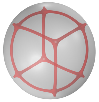
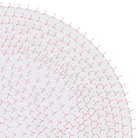
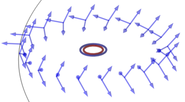
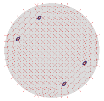
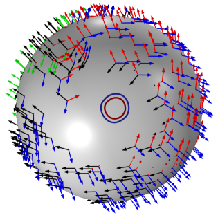
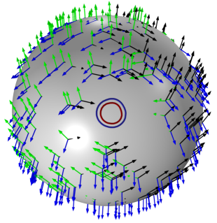
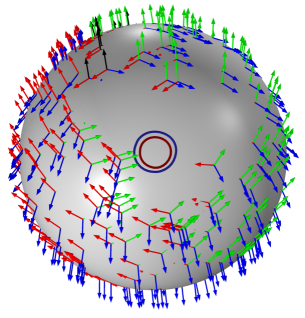
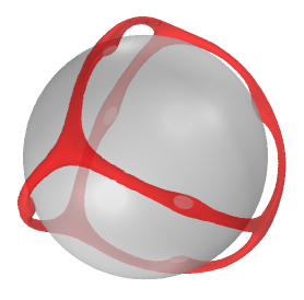
When we constrain a frame field to contain the normal on the boundary for topological reasons singularities emerge, as is in the case of 3-cross fields, [29]. Our variational relaxation approach allows us to observe formation of singularities numerically, Fig. 1, and to study their topological properties. Here unexpected features arise as consequence of noncommutativity of the fundamental group of the target manifold.

In particular, unlike the standard Ginzburg-Landau where the number of singularities is dictated by the degree of the boundary data, here we observe local minimizers with different number of vortices for the same boundary conditions. Further, local minimizers in three dimensional domains exhibit one-dimensional singular sets that meet at triple junctions (as opposed to quadruple junctions in [29]). These junctions and their structure are another novel feature of our numerical experiments. Investigation of properties of minimizers of our relaxed problem is a fascinating challenge for further analysis.
Note that tetrahedral frame fields on can be written as maps , where is the tetrahedral group and the binary tetrahedral group, its pre-image under the covering map . It is well known since the work of F. Klein [43] that the quotient of by a finite subgroup of can be realized as an algebraic variety in , using the theory of invariant polynomials. Because here we are interested in the quotient which is a closed subset of , the Klein construction would require us to impose additional polynomial constraints. Rather than use this approach, we instead embed into an algebraic variety of a Euclidean space of a large enough dimension so that the resulting polynomial equations are of order two, the lowest possible for a non-linear polynomial. As it turns out, this embedding is into a set that can be endowed with a natural matrix structure that leads to nice compactness properties in weak topologies, see [30].
Our interest in tetrahedral frame fields represented by third order symmetric traceless tensors is not purely mathematical as they have drawn significant attention from the physicists since the early 80’s [8, 17, 46, 22, 52, 53, 61]. As we will discuss in the next section, of particular relevance to this work is modeling of bent-core liquid crystals, where phases with tetrahedral symmetry can arise in certain temperature regimes.
1.1. Results and organization of the paper
We now describe the organization of this paper. Section 2 provides necessary background and motivation for our work from the modeling of nematic liquid crystals with symmetries and other physical applications.
In Section 3, we start with vectors, in that are equally spaced out on . Not only does this include tetrahedral frames, it also includes the two-dimensional analog of a tetrahedral frame. This analogous frame consists of the position vectors of vertices of an equilateral triangle with the center of mass at the origin, and we refer to such a three-pronged shape as an MB frame. MB frame fields appears naturally when we discuss traces of tetrahedral frame fields on the boundary of a three-dimensional domain. Associated with the vectors is a symmetric three tensor,
| (1.1) |
The rest of Section 3 identifies invariants of tensors (1.1): not only are the ’s symmetric and traceless, they also satisfy an SVD-type identity,
| (1.2) |
where is the identity matrix and , see Proposition 3.3. Identity (1.2) proves to be a crucial tool, as we will use it to ”push” our linear space towards . Additionally, we show that these ’s enjoy an eigenvector-eigentensor structure, see Proposition 3.6. A particularly useful consequence of the eigenvector-eigentensor pairing is a mechanism to ensure that the normal vector is contained within and MB or tetrahedral frame field,
| (1.3) |
Suppose that is the set of -th order tensors in that are symmetric and traceless, i.e. invariant with respect to permutation of indices and such that a contraction using the last two indices produces a zero -order tensor in . In Section 4 we establish two theorems that enable us to recover frames of interest in two and three dimensions. When we prove that
| (1.4) |
where is the -rotation group. When we establish that
| (1.5) |
where is the tetrahedral group. For tensors in we also provide an algorithm for computing four vectors of a tetrahedral frame from a given tensor. These theorems are proved in Section 4 and Appendix B.
In Section 5 we apply our results from Section 4 to generate a frame field in Lipschitz domains. Simple constructions in this section show that requiring the normal vector on the boundary be included in either an MB or tetrahedral frame induces nonexistence of a smooth frame field in the interior. To avoid this, we work in the linear subspace and push towards the constraint (1.2). Indeed the relaxation procedure is defined by generating a sequence,
where the space is described earlier in the section. This space includes constraints to ensure (1.3) holds, or is satisfied in the limit. In later sections, we examine the limiting via computational experiments and show that MB and tetrahedral frame fields are smooth outside of co-dimension 2 singular sets.
In Section 6 we develop a connection between tetrahedral frames and quaternions in , where are the unit quaternions and is a specific finite subgroup. We show that a natural map from quaternions to symmetric traceless tensors induces an isometric embedding of the space of tetrahedra. We also compute the fundamental group of the space of tetrahedra. As the group is non-abelian, the free homotopy classes are characterized by the conjugacy classes of the fundamental group.
In Section 7 we provide some global geometric information on tetrahedral frame fields in smooth three dimensional domains. In particular an adaptation of the classical Poincare-Hopf theorem to frame fields, see [60], provides a constraint on the total index of the tangential MB field induced by the requirement that the normal vector being contained in the tetrahedral frame field on boundary. If one defines the index of the tangential MB field on the surface as the angular change about a singular point divided by , then this results in a formula,
| (1.6) |
where is the index of the zero, is the set of singularities of the tangential MB field on the surface, and is the genus of the bounding surface, see Remark 7.4. Applying (1.6) to a ball in 3D, one finds , which corresponds to the number of boundary point singularities in simulation in Figure 1.
Section 8 describes typical examples of tetrahedron-valued critical points for both two- and three-dimensional energies obtained numerically via gradient flow. In numerical simulations, the trace of each competitor on the boundary of the domain is assumed to contain the normal to the boundary. Topological obstructions associated with these boundary conditions give rise to formation of both boundary point- and interior line singularities.
In prior sections we have looked at energy minimizing sequences in which the Dirichlet energy is appended with a particular fourth-order nonlinear potential that pushes our linear space towards a tetrahedral (or MB) frame field. In Appendix C we explore the connection between our work and a more general fourth order potential for introduced in [47] to describe bent-core nematic liquid crystals. This potential,
allows for much richer sets of minimizers. We characterize some features of energy minimizers with this more general potential in terms of the and . In fact, we find both MB and tetrahedral frames in three dimensional domains, depending on the values of the parameters.
2. Bent-core nematic liquid crystals
A liquid crystal is a state of matter intermediate between a solid and a liquid in that it retains some degree of order characteristic of a solid, yet in can flow like a liquid. For example, a nematic liquid crystal—typically composed of molecules that have highly anisotropic shapes—possesses orientational order for a certain range of temperatures or concentrations. Two other common types of liquid crystals include cholesterics formed by screw-shaped molecules that exhibit orientational order with a spontaneous twist and smectics where, in addition, to orientational order, the molecules tend to assemble into layers.
Suppose that a nematic occupies the domain . Locally, orientational order can be described by a parametrized probability density function that measures the likelihood that a liquid crystalline molecule near is oriented within a given solid angle in . For nematics, the probability of finding the head or the tail of a molecule pointing in a given direction are always the same, hence for every and .
A practically useful approach to describe a probability distribution over is to generate its moments over the sphere. In classical Landau-de Gennes theory for nematics the invariance of with respect to inversions guarantees that the first nontrivial moment of for every is the second moment
Here the second-order tensor is symmetric and traceless and
for any map defined on . The liquid crystal is in the uniaxial nematic phase if exactly two eigenvalues of e.g., are equal so that
| (2.1) |
where is the degree of orientation of the nematic, is the nematic director and is an eigenvalue-eigenvector pair for . On the other hand, when the liquid crystal has no orientational order and it is said to be in the isotropic phase. The tensor is the order parameter of the Landau-de Gennes variational theory, in which equilibrium configurations of a nematic liquid crystals are assumed to minimize the (nondimensional) energy
| (2.2) |
In this expression, is the orientational elastic energy, is the potential energy, is temperature and is the nematic coherence length. For a thermotropic nematic, there exists a critical temperature such that is minimized by the isotropic phase when while it is minimized by any of the form (2.1) in the manifold of nematic states when . We say that the liquid crystal undergoes an isotropic-to-nematic phase transition at .
The most striking feature of a liquid crystal in a nematic phase are defect patterns of points, lines and walls that can be observed optically under crossed polarizers. Mathematically nematic defects are topological singularities of minimizers of (2.2), associated with the nonlinear constraint . This constraint ensures that (2.1) holds approximately on the entire domain , except for a singular set of a small measure (determined by the size of ) where the tensor is either biaxial or isotropic. Understanding singularities of minimizers of the Landau-de Gennes energy has been a subject of extensive investigations in the last decade [1],[11]-[16], [20, 21, 27, 28, 31, 32], [35]-[38], [42, 48, 54].
A relatively recent discovery of novel liquid crystalline phases formed by bent-core, banana-shaped molecules [40, 41] prompted modifications to the Landau-de Gennes theory to account for symmetries of these phases that do not exist in standard nematics [8, 57, 47, 59]. For example, it has been shown in [47] that an appropriate continuum theory in absence of positional order should depend on the first three moments of an orientational probability distribution of V-shaped bent-core molecules. To this end, suppressing the dependence on , recall that the probability density function can be expanded in terms of powers of by using the Buckingham’s formula [10, 62] written as
| (2.3) |
where
the quantity is the symmetric traceless part of the tensor and denotes tensor contraction. By isolating the first three terms in (2.3) we obtain
| (2.4) |
In this expression, the first moment is the polarization vector, the second moment is the -tensor defined in (2.1) and the third moment describing tetrahedratic order is given by the third order tensor with components
Note that at fourth order, we retrieve a tensor that is useful in describing an ordering with cubic symmetry considered in [18, 29].
The appropriate Landau-de Gennes free energy functional can be constructed as a rotationally-invariant power series expansion around the isotropic state in the order parameters , and and their gradients. The contribution from the gradients of the order parameter fields is the elastic energy while the remaining terms that do not vanish in a spatially homogeneous material comprise the Landau-de Gennes potential. The coefficients of this potential, in general, are temperature-dependent and thus they control the structure of the minimal set of the potential, or the phase in which the material is observed at a given temperature. Given that the bent-core liquid crystals are described by three order parameters, there is a large number of possible phases that form via interactions between different material symmetries. For example, nematic order described by the standard second order tensor may induce tetrahedratic order described by the third order tensor and vice versa via appropriate coupling terms [47]. If one were to neglect the contributions from lower order moments and , the form of the Landau-de Gennes energy for bent-core liquid crystals for third order tensor fields [47] with the potential
is a more complex version of the relaxed energy functional considered in this work. Because both functionals would require identical algebraic and analytical tools to obtain rigorous mathematical results, the present work can serve as a first step toward understanding of the Landau-de Gennes models for third-order tensors in higher dimensions. As a first step in this direction, inspired by [47], in Appendix C we rigorously describe the minima of . Note that recent analysis results [2, 25, 26, 65] have not considered phases of bent-core liquid crystals with tetrahedral symmetry.
3. Symmetric, traceless 3rd order -tensors
3.1. Notation
We will define a series of sub and affine spaces based on a set of vectors . For a given vector , we can write it component-wise, . Let denote the canonical basis in . Let be the set of all -vectors with entries from a ring . We will frequently drop when the dimension of the vector is clear. In particular, .
Let be the set of all matrices with entries from a ring . In particular, . For a square matrix with entries in , we write . We denote elements with capital letters. One particularly important class of matrices for us are projections for a unit vector with . We also denote the identity matrix, .
We next define generic -th order tensors
with elements that have indices for with script letters. We finally define symmetric -order tensors as
where is the group of permutations of -length words. Finally, we define set of traceless, symmetric -order tensors
| (3.1) |
Given this notation, we now describe the specific class of third order tensors that we will study.
Remark 3.1.
We define an especially useful bijection , where for any choice ,
| (3.2) |
This bijection identifies a canonical element of with an element of , and vice versa. Given this bijection, we will frequently refer to elements in and interchangeably.
Likewise, we define the bijection by
| (3.3) |
for As with the prior definition, we will refer to elements in and interchangeably.
3.2. Elements of generated by a frame with -hedral symmetry
We say a collection of vectors has ”-hedral symmetry” if the following condition holds:
| (3.4) |
Such collections satisfy the following result.
Lemma 3.2.
Suppose we have vectors satisfying (3.4), then
| (3.5) |
In particular, the vectors span . Furthermore
| (3.6) | ||||
| (3.7) |
where denotes the projection matrix generated by .
Proof.
To prove 3.5 we consider for example , and consider scalars such that
Taking the dot product of this with , , gives
This can be written in matrix form as follows:
where we use the notation . It is easy to check that is a rank-1, orthogonal projection matrix. Hence, the matrix is invertible. It follows that , so , are linearly independent.
Next, since span then for some constants . This implies
Finally, we choose . Since the frame spans then (3.6) implies we can write for unique constants . Therefore,
∎
We associate with these vectors a third order tensor , defined as
| (3.8) |
For simplicity, throughout this section we write to denote the -th submatrix of . This tensor generated by a set of vectors such that (3.4)-(3.5) hold, satisfy the following identities:
Proposition 3.3.
Proof.
3.3. Linear algebraic results for and
Our first results provides a minimal representation for the unknowns in our space of symmetric, trace-free 3-tensors in dimensions. This will be used in later sections for numerically computing tetrahedral frame fields.
Lemma 3.4.
Let denote the number of variables then the number of unique monomials in is
| (3.13) |
Proof.
Note that the number of monomials of degree 3 of variables is . There are additionally constraints, since , so the total number of unique elements is
∎
We conclude with a few results on vector / matrix pairings that our tensors satisfy. We will discuss these identities in the context of eigentensor-eigenvector pairings in Subsection 4.2. The following result was established by Qi [58] in the case of . We generalize the result to arbitrary dimensions here.
Proposition 3.5.
Let with nonzero singular values. There are matrices , , unit vectors , , and scalars , , such that
and
Proof.
Let us first notice that , so there is such that
where is a diagonal matrix. Furthermore, is non-negative definite. Hence we can call the elements of its diagonal
due to the assumption on the singular values. Let now
and define
By construction, , and if we write , then , and
By the first claim of Proposition 8.1 of the main draft, we have
so
To finish the proof we remember that equation 8.7 of the main draft tells us that
Defining , and , we obtain the conclusion of the proposition. ∎
If we consider three tensors generated by (3.8) via vectors satisfying (3.6), then we can get explicit eigenvector-eigentensor pairs.
Proposition 3.6.
For every there exists an matrix, such that the following holds. For any set of unit vectors in , , that satisfy the inner product condition (3.4), and its associated 3-tensor generated by these ’s via (3.8). Let where the are defined by
If we denote the matrix whose columns are the vectors . Then, the matrix
is orthogonal, and . Letting , , and
where
then, the vectors along with the tensors , are eigenvector-eigentensor pairs for in the sense of Qi (see Remark 3.7). In particular,
Finally, one can recover the -tensor from the eigenvector-eigentensor pairs, in the sense that
for .
The proof of this proposition can be found in Appendix A.
Remark 3.7.
When , the vectors and tensors form eigenvector-eigentensor pairs that are identical to those of Qi:
| (3.14) |
where the eigenvalue .
3.4. Rotations and tetrahedral frames
To conclude this section, we introduce two canonical tetrahedral frames that will be utilized below: and . The first set of vectors includes a vector aligned with :
There is an additional set of canonical vectors typically associated with four vertices on a cube:
| (3.15) |
In both cases, , and so the corresponding three tensors or enjoy the results of Proposition 3.3. One can rotate the set of vectors into with the rotation matrix,
More generally, we can rotate into any tetrahedral configuration on from either canonical set of tetrahedral vectors. In particular, for a rotation matrix, , and permutation operator on four elements, . The corresponding three-tensor satisfies
where
is an element of . We will use this rotational perspective in the proof of the recovery.
4. Recovery of -hedral frame in dimensions
In this section we show the converse of results in Subsection 3.2, namely that elements in with a specific nonlinear constraint produce unique -hedral frame fields.
4.1. Tensors in and MB frames
Focusing on , we show that the identities developed in Subsection 3.2 are necessary and sufficient to uniquely describe the associated -frame. These frames are characterized by three planar vectors with equal -angles between. Given the shape, they are commonly referred to as Mercedes-Benz frames, though we will refer to them as MB frames. Given its structure, it is sufficient to provide a single angle in to fully characterize the frame. Our result in this subsection is
Theorem 4.1.
The following diffeomorphism holds:
| (4.1) |
where is the -rotation group.
Proof.
Consider three vectors that are rotations of each other. If we let
denote and rotation, and if denotes the angle off the -axis, then an MB frame can be described by three vectors
| (4.2) |
Consequently, . Recalling our definition then Proposition 3.3 and Lemma 3.4 imply is a symmetric, traceless 3-tensor with two unique elements, which implies it can be written as
| (4.3) |
where . Since is part of the frame, then (3.12) implies
As a consequence, , , and so
| (4.4) |
Tensor (4.4) recovers the expected three-fold symmetry of the MB frame in two dimensions, and it also provides an explicit representation for boundary alignment of a frame field, as will be discussed later.
We now consider the converse. Suppose with then the representation (4.3) and its nonlinear constraint implies . Consequently,
| (4.5) |
for some angle . Now, assuming that some vector is part of the MB frame, and if returns the unique angle in associated to the ordered pair off the -axis, then (4.4) implies
| (4.6) |
Therefore, our tensor is determined by a unique angle , and since that angle retrieves the other two vectors by and rotations of the vector associated to (4.6), we retrieve the full MB frame. ∎
4.2. Tensors in and tetrahedral frames
We turn to and show our the identities are necessary and sufficient to uniquely describe an tetrahedral frame. Our result is
Theorem 4.2.
We have the following diffeomorphism:
| (4.7) |
where is the tetrahedral group.
More explicitly, for every there are vectors , , such that
and such that
The four vectors are the four unique maximizers of
| (4.8) |
Proof.
Given four tetrahedral vectors, the corresponding tensor lives in due to our results in Section 3. The converse is much more involved, and its proof can be found in Appendix B. ∎
Remark 4.3.
Note that in [24] eigenvalues and eigenvectors in the sense of [58] were obtained for third order symmetric traceless tensors by maximizing the so-called octupolar potential
The potential is different from in Theorem 4.2. Both and have exactly the same maximizing set when , however the maximizing sets no longer coincide for .
5. Ginzburg-Landau relaxation to the appropriate variety in 2 and 3 dimensions
Since MB and tetrahedral frame fields can be identified by nonlinear sets in for , we propose a Ginzburg-Landau relaxation towards these constraints. This procedure leads to a direct method for generating these frame fields on Lipschitz domains.
5.1. MB Frames:
MB-frame fields are an example of an -direction field, in which each point in domain or tangent to a surface (see Section 7) is assigned evenly spaced vectors, see the review article [63] for background on this topic. We now show how our framework generates an MB-frame on a two dimensional domain, outside of small number of singular sets and reduces to methods similar to those found in [3, 64] for 2-cross fields.
By Theorem 4.1, we can uniquely represent our MB frame field by an element of . However, not all maps with boundary data in extend smoothly into the interior.
In particular from Theorem 4.1 we let
and if , then where . Therefore, our MB frame can be generated by determining angle and computing the other two vectors by and rotations of the vector associated to .
Definition 5.1.
Let be a map with with except at isolated points, and for some . For a simple closed curve not meeting any of the zeroes, we define the index of on by finding a continuous lifting via the universal cover, , with and setting
The index of an isolated zero is defined as that of on any closed, Jordan curve surrounding (in a counter clockwise manner) and no other zeroes. We denote the index about this as
It is standard that the index just defined takes values in , compare [33, p. 108] for the case . We often use the words index, degree and winding number interchangeably.
For this reason, instead of looking for smooth extensions of boundary data, we relax towards using the variety associated to this quotient. In particular we look for such that is satisfied on the boundary, and the normal is a part of an MB frame. We can, therefore, define the space
i.e. the normal, , is part of the MB frame. If the normal is smoothly defined on the boundary, it induces nontrivial topology in , due to (4.4), and this can preclude globally defined MB frame fields. In particular, by the constraint we can set with and on . Setting
then we can try to minimally extend the boundary data into the interior subject to (4.4), which entails minimizing
However, by classical arguments for any domain topologically equivalent to a disk.
To avoid such problems, we relax towards the manifold . In particular we take a sequence and penalize the distance from the variety by looking for minimizers of the associated Ginzburg-Landau functional,
| (5.1) |
We then consider a sequence
subject to the boundary conditions that have normal as a part of the MB frame which, in turn, induces the dependency.
The condition that competitors on the boundary are MB frames containing the normal to can also be enforced in a weak sense by introducing the surface energy term that penalizes deviations from this condition. With the help of (3.12), the surface energy can be taken in the form
| (5.2) |
so that the energy functional is
| (5.3) |
The interplay between the parameters and will be discussed in Section 5.4 in the case of tetrahedral frames.
5.2. Tetrahedral Frames:
We now turn our attention to foliating a Lipschitz domain with tetrahedral frame fields. Using Theorem 4.2, this is equivalent to looking for harmonic maps in . However, as in the 2D problem, this manifold typically generates singularities due to boundary conditions, and so we will use a harmonic map relaxation with prescribed boundary conditions.
Suppose that with , we define the operator via
| (5.4) |
then by (4.8) in the proof of Theorem 4.2, the four vectors which maximize (5.4) define a unique tetrahedral frame in . Therefore, we can generate a tetrahedral frame field by filling our domain with harmonic maps in and generate the tetrahedral vectors at each point in the domain using maximizers of . However, as in the MB frame field situation, if we look to fill out our Lipschitz domain with tetrahedral frame fields that adhere to the boundary, we find topological obstructions. The challenge, again, is the nonlinear constraint, and so we again relax towards the nonlinear constraint using a different nonlinearity.
We now describe this procedure in detail. From (3.13) a general has the . Letting allows us to express
and our potential
| (5.5) |
Before generating the associated Ginzburg-Landau energy, we need to provide suitable boundary conditions that ensure the normal vector is included in the tetrahedral frame.
5.3. Boundary conditions and reduction to the MB frame
In order to prescribe natural boundary conditions of the tetrahedral frame, we impose that the normal on the boundary comprises one of the four vectors of the frame. Consequently, we arrive at the following conditions on the frame at the boundary, due to (3.11) and (3.12):
Lemma 5.2.
If is a normal on the boundary and an element of the tetrahedral frame , then
Equivalently, if is the outer normal on the boundary and an element of the tetrahedral frame , then
| (5.6) |
Here, for an matrix , is the vector in that contains the columns of vertically, in order, and .
If this holds for , then we can solve for using the underdetermined system of equations
| (5.7) |
In particular, the matrix on the left has rank 5.
If we assume the boundary is locally then is an element of the frame. We can then locally parametrize the orientation by planar rotation of . The corresponding becomes:
Furthermore, condition (3.10) implies or
Given the three-fold symmetry of the remaining three vectors of the tetrahedral frame implies a direct analogue of the MB frame result:
5.4. Relaxation
We can now consider a harmonic map relaxation to the tetrahedral frame field using a Ginzburg-Landau formalism. We first set
For elements of , we define a relaxed energy,
| (5.8) |
and consider
As pointed out in Lemma 5.2, the condition that the normal to the boundary is part of the tetrahedral frame can be conveniently imposed by assuming that
This condition could also be imposed in a weak form through a boundary integral. This leads us to the alternative energy
| (5.9) |
where
For our next result, we will use the notation
for the orthogonal projection from the set of rank-3 tensors onto the our relaxation space .
Proposition 5.3.
Let . The critical points of the energy satisfy
independent of .
Proof.
First we observe that the Euler-Lagrange equation along with boundary conditions for the energy are
Here,
and
denote the gradients of the potentials with respect to , and , .
Now, since , we have . We also have , so we can estimate
| (5.10) |
Next, for , and using the facts that , , , we obtain
| (5.11) |
Now, we take the inner product of the equation satisfied by with , and use (5.10), to obtain
On the other hand, using 5.10 and 5.11, and writing , we obtain
From here we obtain
From the equation satisfied by , and Hopf Lemma, we conclude that . This is the conclusion of the Proposition.
∎
Before we use this formalism to generate tetrahedral fields for different Lipschitz domains in two and three dimensions, we first discuss the topology of and its effect on the frame field.
6. Tetrahedral frames and quaternions
In this section we discuss how tetrahedral frames can be described using quaternions as , where are the unit quaternions and is a specific finite subgroup. We show that a natural map from quaternions to symmetric traceless tensors induces an isometric embedding of the space of tetrahedra.
We compute the fundamental group of the space of tetrahedra, following [51]. As the group is non-abelian, the free homotopy classes are characterized by the conjugacy classes of the fundamental group, compare also [49], [61] for similar topological considerations in theoretical physics.
6.1. Quaternions, rotations and tetrahedra
It is a well known result that the group of unit quaternions can be used to describe rotations in . The following lemma is standard:
Lemma 6.1.
Set for , then
with is a group homomorphism with kernel .
Proof.
Note that is the matrix representation of the map for a pure quaternion identified with a vector in . It is an easy computation that is a pure quaternion and the matrix is orthogonal. ∎
We now define some useful groups: The tetrahedral group is the subgroup of that map the standard tetrahedron defined in (3.15) to itself, i.e. where is a permutation. It is well known that is isomorphic to the alternating group : rotations preserve the orientation so cannot generate any transpositions. On the other hand, any -cycle in can be generated as a rotation around the leftover vector. Finally, we have the binary tetrahedral group , given by
where each of the represents an independent choice so there are elements in total. It is generated by and , which satisfy .
Lemma 6.2.
The map induces a map that acts as follows on the standard tetrahedron:
so there is an induced map that has the following representation:
Proof.
This is a straightforward computation. ∎
We see that the tetrahedral group is composed of rotations around of the vectors of the tetrahedron (these correspond to the -cycles) and rotations around the axis going through the midpoints of two opposite edges (these correspond to the products of two transpositions). The binary tetrahedral group has twice as many elements, and we have the following characterisation of its conjugacy classes:
Lemma 6.3.
There are seven conjugacy classes of elements of :
| Elements | Geodesic distance from | description |
|---|---|---|
| identity | ||
| 1/3 rotation around one of the tetrahedral vectors | ||
| -1/3 rotation around one of the tetrahedral vectors | ||
| -1/3 rotation around one of the tetrahedral vectors | ||
| 1/3 rotation around one of the tetrahedral vectors | ||
| full rotation | ||
| rotation interchanging two pairs of vectors |
Proof.
We note that powers of are conjugate to each other if and only if they are the same, which gives that the classes corresponding to . are all separate. Conjugating each of these elements with , , yields the rest of the conjugacy class. The elements form their own conjugacy class because the geodesic distance to is invariant under conjugation and we can compute and etc. ∎
The configuration space of regular tetrahedra with vertices on the unit sphere can be understood as follows. Let
and , where acts by permuting the indices. Then contains all collections of oriented tetrahedra with indexed vertices and the corresponding collection without numbered vertices.
Proposition 6.4.
We can identify .
Proof.
We can map into by considering the action on a fixed standard tetrahedron. The image of two rotations in is clearly the same iff they differ by an element of . To see that this map is surjective, note that for any , we can choose such that for , by first rotating into and then rotating around this axis to align the other vectors.
That is almost the definition of , the preimage of under the double covering . ∎
6.2. Embedding of tetrahedra into tensor spaces
Our main result in this subsection establishes an isometry between and our tensor space .
Theorem 6.5.
Taking the vectors of a standard tetrahedron, , given in (3.15), we can generate the -rotated tetrahedron
| (6.1) |
The map given by is up to scaling a local isometry in the sense that it satisfies for all and , the tangent space, where .
The induced map is well-defined and injective, and up to scaling we find an isometry .
Proof.
The heart of the matter for proving the local (scaled) isometry character is to use that is a group, so it suffices to show this for . Writing a geodesic through as for , we have and . Let , be the four unit vector of a tetrahedron. We compute
Using and yields
For , we note that
because , and . So far then we have
However, again using the fact that , we obtain
Putting everything together, we then conclude that
This is a multiple of . The parallelogram identity then implies that is (up to scaling) a local isometry.
If then by Theorem 4.2 we have that so and , so is well-defined and injective on . It is surjective by Theorem 4.2.
∎
6.3. Homotopy of the set of tetrahedral frames
With our identification of the space of tetrahedra as , we can now determine its fundamental group:
Proposition 6.6.
The fundamental group of the space of tetrahedra is .
Proof.
The definition of means that its elements are represented by homotopy classes of (continuous) loops where the homotopy keeps the start/end point fixed. The following result considers also free homotopies where the start/end point is not fixed throughout the homotopy.
Proposition 6.7.
If are loops in starting and ending at , then and are (freely) homotopic to each other if and only if their homotopy classes are conjugate, i.e. if there exists with
Proof.
This is a standard result in elementary algebraic topology, see e.g. [9, Proposition III.2.4]. ∎
As the identity is the only elements in its conjugacy class, it follows that for simply connected , a has an extension if and only .
For boundary conditions that cannot be resolved by a globally continuous map, it is possible to find ”topological resolutions”. The following is a special case of the treatment in [51, Section 2.1].
Definition 6.8.
Let be a simply connected sufficiently smooth domain in and let . A collection of maps is called a topological resolution of if there exist distinct points and such that there is with on and on each copy of .
Proposition 6.9.
Let be a simply connected sufficiently smooth domain in and let . A collection of maps is a topological resolution of if and only if there exist such that the homotopy classes of and of satisfy
i.e. iff a conjugate of the homotopy class of the outer boundary map can be written as a product of conjugates of the homotopy classes of the inner boundary maps .
Proof.
This is a slight reformulation of the simplest case of [51, Proposition 2.4], adapted to our special case. We refer to that article for a discussion about the independence of this result from the order used in the product. ∎
Remark 6.10.
There are several possible topological resolutions of the identity with different numbers of homotopy classes at geodesic distance : We have a length zero resolution , a length resolution and a length resolution . From these we can construct arbitrary longer resolutions. Note that gives another resolution. For this reason, in numerical simulations we observe local minimizers with higher number of singularities than what is expected for a global minimizer. The same phenomenon has been observed in the Landau-de Gennes context for -tensors describing nematic liquid crystals, where local minimizers with singularities were rigorously shown to exist [39] for topologically trivial boundary data.
6.4. Generating data in free homotopy classes of tetrahedral frames
Armed with the results of the previous subsection, we can now try to interpret tensor-valued maps with target into except for a finite number of point singularities as topological resolutions of their boundary data.
To construct a map with given homotopy types, we can use the following recipe:
Definition 6.11.
For , we set and let
with and .
Proposition 6.12.
The satisfies with , . is a smooth geodesic.
For the formula reduces to the following cases:
If then
For ( and are analogous):
If then
Proof.
This is a straightforward computation. ∎
Lemma 6.13.
Let , . Then the map ,
induces after taking the quotient modulo a topological resolution of its boundary map. The homotopy class of the outer boundary map is and the homotopy class of the inner boundary is .
Proof.
We need to show that induces a continuous map. This follows after taking the quotient from the fact that , with .
∎
Proposition 6.14.
Let and distinct points. Let be a Möbius transformation mapping to . Then
induces a topological resolution of its boundary data of homotopy type .
Post-composing this with the map of Theorem 6.5 leads to a corresponding resolution in the space of tensors.
Proof.
This is a direct consequence of the preceding computations. ∎
7. Poincare-Hopf for MB frame-valued maps on generic surfaces
In this section we recall a version of the Poincare-Hopf theorem adapted to our situation. This theorem can be easily adapted from page 112 of Heinz Hopf’s book [33]. Similar results have been shown to be valid for cross-field-valued maps, [3, 4, 23, 60]. Theorem 7.3 below will be useful in interpreting our numerical simulations in Section 8.
Let be a closed, smooth, orientable surface with normal , and fix an integer , . Consider the set
For , , define the equivalence relation
Define then
In other words, we consider the unit tangent bundle of , and identify tangent vectors that are related to each other by a rotation of an integer multiple of about the normal. Let also be the projection onto the first coordinate.
Definition 7.1.
Let be a finite set. An -gon valued field on is a continuous map such that for every .
In the above definition, if and the field cannot be extended to by continuity, we say that is a singularity of . Next, if is a singular point of , we can define its index.
Definition 7.2.
Let be a singular point of . Consider a closed, continuous curve surrounding , small enough to be contained in a single coordinate patch, and such that is the only singularity surrounded by . Consider a continuous lifting of along through a unit tangent vector, in the sense that, at every point in , can be obtained rotating the unit vector by , times. Compute the angle between this unit vector and one of the coordinate tangents. The total change of this angle as we travel through once anti-clockwise, divided by , will be called the index of the singularity and denoted .
Note when , this definition agrees with Definition 5.1. In particular the index of a singularity in this case is of the form for some integer . Furthermore, as pointed out in Theorem 1.3, page 108 of [33], the degree does not depend on the curve nor on the coordinate patch used to define it. With this terminology we can now state the following theorem. Its proof can be found in page 112 of [33], for the case , or in the appendix of [60], for any . Hence, we omit it.
Theorem 7.3 ([33, 60]).
Let be a closed, smooth, orientable surface, a finite set, and an -gon-valued field in . We assume further that every is a singularity of . Then
Here is the Gauss curvature of , and denotes the index of the singularity .
Remark 7.4.
By the Gauss-Bonnet theorem,
where and are the genus and Euler characteristic of , respectively. Hence, we conclude that
| (7.1) |
8. Examples and numerical experiments
In this section we discuss nontrivial examples of tetrahedron-valued maps, either constructed analytically or obtained via numerical simulations. In the latter case, the goal is to understand behavior of local minimizers of (5.1) and (5.9), respectively by simulating gradient flow for each energy using the finite element software COMSOL [19]. Note that the two analytical examples below only provide competitors and not minimizers of the corresponding variational problems.
8.1. Example of a map from into
Here we show that, similar to what is known for -tensors, normal boundary alignment of tetrahedron-valued maps in two-dimensional domains does not require singularities. Indeed, we can construct a map that is nonsingular because it ”escapes into the third dimension” in the interior of the domain.
On the unit disk with polar coordinates define
Now set
and define
This gives
| (8.1) | ||||
It is easy to check that the map that sends a point in the unit disk to is tetrahedron-valued, nonsingular and the vector coincides with the normal on the boundary of the disk.
Note that a quaternion representation of the rotation inherent in this map (starting from the tetrahedron containing ) is given by
As this is a smooth map into , it belongs to the trivial homotopy class.
8.2. Example of a map from into
The next example is that of a tetrahedron-valued map on the unit ball in that has exactly one point singularity on the boundary of the ball (at the north pole) and no other interior point or line singularities. This map also has a finite Dirichlet integral. The example is a straightforward adaptation of a similar computation for orthonormal frame-valued map in [29].
Let , then define the vector fields
for , . Note that , and whenever . It follows that is an orthonormal frame for the tangent plane at the boundary whenever .
Next set
then for . Further, that is the map that sends to is MB-valued in . By construction, the two-dimensional MB frame is contained in the tangent plane at any .
Similar to the previous example, now let
so that
A straightforward computation shows that, for , we have
Thus the vectors give the 4 vertices of a tetrahedron and we can consider the map that sends to the tetrahedron defined by . Since and for , one of the vectors of this tetrahedron coincides with the normal on the boundary of the unit ball.
8.3. An energy-minimizing map from into
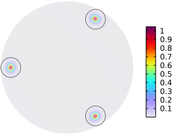
Here we examine an MB-frames-valued map generated by a gradient descent of the energy (5.1) subject to the Dirichlet condition that the normal on the boundary is aligned with the MB frame. When simulating in a domain that has a shape of an equilateral triangle, the gradient flow converges to a constant state with the three vectors of the MB frame perpendicular to the respective sides of the triangle. Clearly this state is also the global minimizer of (5.1).
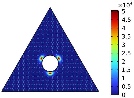
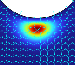
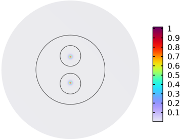
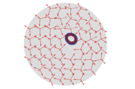
In order to observe a state with vortices, we excised a disk from the equilateral triangle. The restriction of the solution to the boundary of the triangle is still a constant MB frame, while the requirement that the normal to the boundary of the disk is aligned with the MB frame produces winding of the normal by the angle when the boundary of the disk is traversed once in the positive direction. Because the quantum of winding for the MB frame is (as the degree takes values in ), we thus expect three vortices with opposite of that winding to form in the interior of the domain. Indeed, in Figure 2a one sees that an MB frame aligns with the exterior boundary away from the excised disk, while the disk induces three vortices with winding of (Fig. 2b).
8.4. Computational examples of maps from into
We now explore critical points of (5.8) for two different choices of Dirichlet boundary conditions.
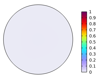
(a.) First, consider a tetrahedral frame field defined by the vectors given in (8.1) and consider critical points of the energy from (5.8), that satisfy the same Dirichlet data as . We first run the gradient flow simulation for this setup assuming the the initial condition is also given by . Because is smooth in and the energy of the gradient flow solution is bounded by its initial value, the critical points obtained starting from have energies that are uniformly bounded in so that the critical point is nonsingular (Fig. 3).
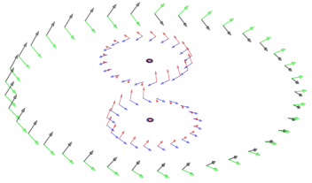
On the other hand, the gradient flow simulation that starts from the trivial initial condition results in an entirely different stable critical point shown in Fig. 4. This local minimizer has three equidistant point singularities such that the frame field over any curve surrounding one singularity is in a homotopy class conjugate to either or , i.e., one vector of the frame does not change while a curve is traversed, Fig. 4(b)-(d).
The different critical points, given the same boundary data, is an example of distinct topological resolutions for that data, see Remark 6.10.
(b.) The next example shows a critical point of (5.8) obtained via a gradient flow in a unit disk for maps satisfying Dirichlet boundary data that lies in a homotopy class conjugate to . Here both the boundary and the initial condition were obtained using the techniques described in Section 6.4. The initial condition had a singularity at the center of the disk and the tetrahedral frame map was in the same homotopy class as the boundary data for every circle surrounding the singularity. The simulation attains a local minimizer of (5.8) shown in Fig. 5. This minimizer has two singularities in the interior of the disk and examination of winding of the frame vectors indicates that the frame field over the curves surrounding each singularity has a homotopy class conjugate to . Indeed, the state with two singularities corresponds to a shorter topological resolution than that for the boundary data and thus this state has a lower energy than a state with one singularity.
The two remaining examples deal with the tetrahedron-valued maps obtained via a gradient flow for the energy (5.9) when
8.5. Computational examples of maps from into
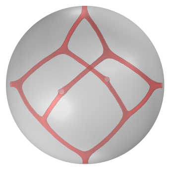
(a.) In Fig. 6c we depict the singular set of a critical point of (5.9) in the ball of radius , where the surface contribution to the energy forces the tetrahedron-valued map to contain the normal to the sphere almost everywhere on . Then the trace of this map on can be identified with an MB-valued map. From Remark 7.4, it follows that any MB-valued map must have singularities on with the degrees of these singularities adding up to . Notice that the energy of an MB-frame field in (5.1) is identical to the scaled Ginzburg-Landau energy after a short calculation. Recall that in Ginzburg-Landau theory, vortices of higher degree in equilibrium split into vortices of degree that repel each other, [6], and we expect analogous behavior from vortices of MB-valued maps. Because the degree of the MB-frame is measured in units of , the singular set of total degree on the sphere should split into six equidistant vortices of degree .
Since we assumed that , the penalty associated with the surface energy is much stronger than that for the bulk energy and therefore the surface effects should dominate bulk effects. Indeed, the singular set in Fig. 6c(a) intersects the surface of the sphere at six, approximately equidistant points, connected by line singularities in the interior of the domain. The bulk structure of the singular set is dictated by the topology of and the energy considerations. In particular, from Fig. 6c(a) it seems to be clear that the total length of the singular set can be reduced by “squeezing” it toward the center of the ball. This, in fact, is possibly what would happen as but such investigation is beyond the scope of the present paper. Rather, we are interested to understand the behavior of the singular set for finite and by exploring the topological structure of a triple junction.

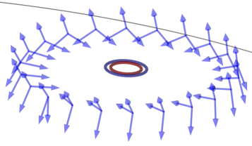
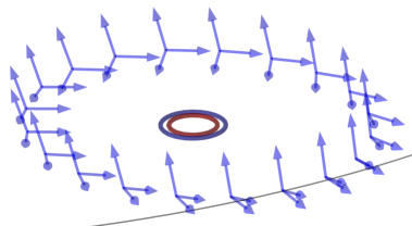
In Fig. 7(a), a small sphere surrounds the triple junction that we are interested in and in Fig. 7(c) we plotted the vectors of the trace of the tetrahedron-valued frame field on the surface of that sphere. The circles on the same plot depict the intersection between the singular set and the surface of the sphere.
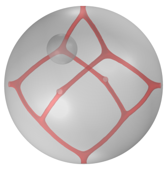
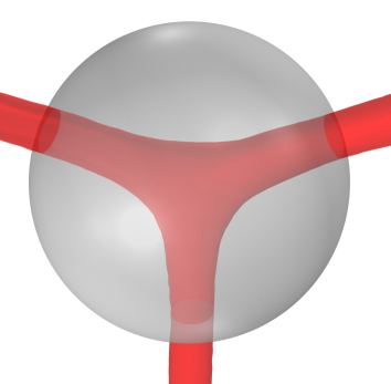
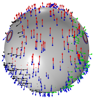
Fig. 8c shows the same small spherical cutout from the points of view of individual arms of the triple junction. Near each singularity on the sphere associated with an arm of the junction, a frame vector of one color points into the sphere toward the triple junction and is not visible, while the remaining three vectors form an MB frame field. This MB frame field rotates by counterclockwise when one travels around the singularity in the counterclockwise direction. The product of two counterclockwise rotations around any two adjacent edges of a tetrahedron indeed corresponds to an inverse of a counterclockwise rotation around a third edge and we expect that a similar structure is valid for the remaining triple junctions of the singular set in Fig. 6c(a).
(b.) Finally, in Fig. 9 we show the singular set of a critical point of (5.9) in a large domain in the exterior of the ball of radius , where the surface contribution to the energy forces the tetrahedron-valued map to contain the normal to the sphere almost everywhere on . The structure of this set is clearly similar to that in Fig. 6c in that it has six equidistant vortices on the surface of the sphere and the same number of triple junctions but, this time, the total length of the line singularities composing the singular set can be reduced by compressing these singularities towards the sphere. This is indeed what is observed in Fig. 9.
9. Discussion
Tetrahedral symmetry arises in many contexts in nature, including in liquid crystals, condensed matter physics and materials science. The framework presented here for generating such frame fields entails identifying a bijection between a tetrahedral configuration and a specific variety on traceless, symmetric three-tensors. When tetrahedral frame fields are constrained to align with the normal, singularities arise generically. To avoid this, the variety suggests a natural harmonic map (Ginzburg-Landau) relaxation that helps in computation to identify a local minimizing configuration with isolated near-singular sets. We discuss some open questions and interesting lines of inquiry related to the work presented here.
In Section 3 we showed that vectors satisfying -hedral symmetry on the unit sphere in defines a symmetric three tensor that satisfies . On the other hand, the recovery has only been shown for . In particular it would be natural to ask if for all there is a bijection between and , where represents the group of rotations leaving equipositioned points on the sphere invariant.
There are many other interesting directions to explore. Recently, it was proved that the energy density of mappings from planar domains into relaxed vacuum manifold targets converge to a sum of delta functions with masses associated to the energy minimized over all nontrivial homotopy classes (so-called systolic geodesics), see [50, 51]. One interesting direction would be to perform a stability analysis of equivariant critical points that conform to different homotopy classes either on the boundary of a disk or at infinity, along the lines of [39] for -tensor models. This should provide additional information on the selection of particular topological resolutions found in our numerical experiments. Even more more important would be to rigorously establish the expected Gamma-limit of the relaxation energy, (5.8). In particular, one should be able to identify a compact mapping, along the lines of the Jacobian in Ginzburg-Landau theory, that concentrates at singular points for two dimensional domains and co-dimension two, rectifiable sets for three dimensional domains. Results for the cross-field case are the subject of the work in [30], and we expect the Gamma-limit in the tetrahedral frame problem to behave similarly.
A more intriguing task would be to provide a rigorous rationale for the formation of triple junctions in the singular limit of tetrahedral frame fields for mappings on three dimensional domains (versus quadruple junctions in the case), see Fig 1. Systolic geodesics should play a role here.
Even more generally, one can ask how this approach can be used to connect a quotient of a Lie group with a specific choice of symmetric tensor and a variety. For example can a frame with icosahedral symmetry, , be generated by a suitable variety on the correct choice of -symmetric tensors? How these ’s and choice of varieties arise remains mysterious.
10. Appendix A: Proof of Proposition 3.6
In this section we prove Proposition 3.6. This requires the use of properties of families of vectors in that we recorded in Lemma 3.2, particularly the property stated in (3.7). For the convenience of the reader we first state the Proposition, and then proceed to its proof.
Proposition 10.1.
For every there exists an matrix, such that the following holds. For any set of unit vectors in , , that satisfy the inner product condition (3.4), and its associated 3-tensor generated by these ’s via (3.8). Let where the are defined by
If we denote the matrix whose columns are the vectors . Then, the matrix
is orthogonal, and . Letting , , and
where
then, the vectors along with the tensors , are eigenvector-eigentensor pairs for in the sense of Remark 3.7. In particular,
Finally, one can recover the -tensor from the eigenvector-eigentensor pairs, in the sense that
for .
Proof.
For the proof we first construct the matrix , and proving several of its properties. The conclusions of the Proposition will then follow from here.
Step 1. In this step we will build an matrix , , such that , that
and , where we use the notation
The construction of is inductive, starting with . Let
and let be the columns of . It is straight forward to verify that
It is also straight forward to check that .
The last two properties of that we need are the following:
The first of these comes from the fact that the rows of , thought of as vectors in , are orthogonal to each other, and have length . The second comes from the fact that the entry of is exactly .
Let us now suppose we have an matrix , , such that , that , and that
All these conditions hold for . With all this let us define the matrix
Note that the last row of , thought of as a vector in , is orthogonal to the others by the hypothesis , and its length squared is , whereas the length squared of the other rows is
Since the other rows of are orthogonal among themselves by the hypotheses on , this shows that .
It is also easy to see that each column of has length , and that the dot product of the last column with any of the others is exactly . Since the dot product between two different columns of is , we conclude that the dot product of any two different columns of , not including the last, is
This shows that
Lastly, that follows easily from the form of the last row of and the hypotheses on . This concludes the proof of Step 1.
Step 2. In this step we now consider a family of unit vectors that satisfy the inner product conditions (3.4), and its associated 3-tensor generated by these ’s via (3.8). Let where the are defined by
We will denote the the matrix whose columns are the vectors . It is easy to check that the inner product conditions (3.4) say exactly that
whereas equations 3.6 and 3.7 from Lemma 3.2 say that
Our main claim in this step is the following:
From here it follows that , and .
The proof is straight forward. Indeed, we first observe that
because and .
Next, we notice that
where again we used the fact that .
Step 3. In this last step we build our eigenvector-eigentensor pairs from what we obtained in the previous step, and prove that the -tensor we mentioned at the beginning of the previous step can be reconstructed from these pairs. Our definitions are the following:
where . We need to prove
is direct from their definition and the fact that , whereas is by definition of . To prove the other two we first observe that , which is a direct consequence of equation 3.10 from Proposition 3.3. Then we compute
Next we compute
where we again used the fact that .
Lastly we observe that
This is the statement that the -tensor can be recovered from the eigenvector-eigentensor pairs.
∎
11. Appendix B: Proof of Theorem 4.2
In this section we will prove a useful property of the tensors in our algebraic variety. Let us first recall that
and
Let also denote the identity matrix.
We define a contraction operator on symmetric tensors which is, in effect, the trace over the last two components. For we set the ”block trace” operator, , to be
| (11.1) |
for any . Consequently, if then . The block trace operator will be used extensively in the proof of Theorem 4.2, as it was used in the recovery theorem in [29].
In this section we will think of the set as the set of matrices, and as the set of symmetric ones. For we define the inner product
We then define
by the equation
where denotes the canonical basis in . Notice that
where the inner product in the left-hand side is the inner product in , while the one in the right-hand side is the standard dot product in . In other words, the map is an isometry.
In this section we will also consider an element of the set as a matrices with real entries. For this, we think of vectors , in any Euclidean space, as columns. In particular, for , , is an matrix. Then, for , we identify the tensor with the matrix
With this notation the permutation operators can be expressed as follows: for , so that , and a permutation , define by
and extend to by linearity.
Next recall the block-trace operator in (11.1). It is easy to check that this operator satisfies the condition
This operator considers a matrix as being built from blocks , and sends into a vector containing the trace of in its -th component.
With all this notation in place we can restate the definition of as follows:
| (11.2) |
We now record some properties of tensors that will be important to us. Let us recall that the canonical orthonormal basis of is denoted by .
Proposition 11.1.
Let , and write , where . It holds
| (11.3) |
Furthermore, we have
| (11.4) |
for every . Finally, we have
| (11.5) |
also for every .
Proof.
To prove identity (11.3), for , let , and observe that the rows of the tensor , as vectors in , correspond to the blocks of . Since , by definition we have . This shows (11.3).
To prove (11.4), observe that, owing to equation (11.3), we have
(11.4) follows from this last identity, and the definition of .
Finally, to prove (11.5), recall that by definition
Because of this and (11.3), we have
From here we obtain
where the last equation is because . (11.5) follows directly from here.
∎
It will be useful to have an explicit basis for the space , in terms of the canonical orthonormal basis of . For this, let us define the tensors
associated to the canonical basis . Note that the ’s are rank-, orthogonal projection matrices with orthogonal images, and . We emphasize that these ’s are different than those defined in Section 3. Define also
Observe that the together with the provide a basis for the set of symmetric, matrices with real entries. With all these we now have the following.
Proposition 11.2.
The following list provides a basis for :
Given this notation, the following list is a basis for :
Note that this implies that has dimension .
Next, we will need to work in the set , and we recall that, by Remark 3.1, we identify elements with . With this in mind, we point out that, for we can also define a permutation operator . To define it, let , , define by the condition
and extend it to by linearity. We trust that the use of the same notation for the permutation operators in , and will not be a source of confusion.
There are two families of elements in that will appear naturally in the proof of Lemma 11.8. Here we use the notation from the Appendix of [29]. For two matrices define
| (11.6) |
Observe that
When we will simply write in place of .
Next, again for , let be the matrix defined by the equation
| (11.7) |
Again, when we will write in place of . From [29], we can give an expression for , as follows: denoting , that is, is the entry of , then
| (11.8) |
The next proposition appears in [29]. We include its proof for the reader’s convenience.
Proposition 11.3.
For the permutation , the operator satisfies
| (11.9) |
for every .
Proof.
A simple way to see that the operator indeed has this property is to observe first that by definition
Calling , , and , then clearly
The result of the proposition follows by linearity, and the fact that every matrix in is a linear combination of rank-1 matrices of the form with . ∎
Remark 11.4.
For , and , the definition of reads:
Since every is a linear combination of tensors of the form
it follows from here that
for every .
Next, we again recall the block-trace operator from (11.1). Under the identification of with , this operator can be thought of as , and then it can be defined by the condition
Thinking of the elements as matrices, and we look at such an as being built from blocks, then just adds the blocks in the diagonal of . For this reason we refer to as the block-trace operator
Remark 11.5.
Next, construction a basis for in the spirit of [29]. We recall here that, by Remark 3.1, we identify with .
Proposition 11.6.
For the space
the following list provides a basis:
for . For their block-traces we have
Proof.
The proof of the basis is straightforward and follows from tensor combinations of the ’s in , along with symmetry assumptions in the indices. The block-trace identities likewise follow from the tensor constructions and the contraction of the last two indices. ∎
Remark 11.7.
It is important to notice that in general , whereas . On the other hand depends on the order of the indices ; however, .
The main use of the bases for and will be to prove Lemma 11.8. Indeed, using these bases we will compute , which satisfies for , and write it as a sum of a term that belongs to , and a second term to which we can apply Proposition 11.3. The analysis of these terms will give us the proof of the aforementioned Lemma.
11.1. Block-trace conditions on
A result for permutation invariant -tensors that have traceless blocks and satisfy a normalization condition. Our main result in this section is the following.
Lemma 11.8.
Let , and assume
for some . Then there is such that
where we are using the notation defined in equation (11.6).
Before giving the proof of this lemma we derive a corollary from it that we will need for our recovery argument.
Corollary 11.9.
Let , and assume
for some . Write , where and . Then
for .
Proof.
First observe that . A direct computation shows that . We conclude that , so satisfies the hypotheses of Lemma 11.8.
Next, recall that by Remark 11.3, we can write
Because of this, we obtain
In particular, the hypothesis tells us that
| (11.10) |
Also from Remark 11.3 we obtain the expression
| (11.11) |
By Lemma 11.8 we know that
| (11.12) |
Now recall the operator defined in (11.9). Applying this operator to (11.11) we obtain
We can also apply to (11.12) to obtain
because and (11.12).
To conclude, we observe that
by the definition of given in (11.7). However, we also have
by the definitions (11.6) and (11.7) of and respectively, the fact that , (11.10), and the expression (11.11) for . The last two equations give the claim of the Corollary.
∎
Proof of Lemma 11.8.
The proof consists in computing using structure of the bases for and provided by Lemmas 11.2 and 11.6 to conclude.
Step 1. By Proposition 11.2 we can write as
| (11.13) |
A direct computation shows that
| (11.14) |
We will expand each of these sums.
Step 2. Computation of . By Proposition 11.2 we have
Since , we obtain
From here, by adding and subtracting terms of the form we obtain
Observe that in this expression the first three terms belong to , and have Block-trace equal to zero. In contrast, the last three terms are not permutation invariant, and each has Block-trace equal to a linear combination of the ’s.
The same argument gives us
and
Finally, we also have
Step 3. Computation of , .
First we observe that
We now add and subtract terms of the form to obtain
Observe again that the two terms on right hand side of the first line are Block-traceless, permutation invariant, whereas the term in the second line is not. We also have
and
Step 3. Computation of . With the same logic we have used so far we have
and
Step 4. Consequences of . From all our previous computations we now have the following:
From we deduce that the coefficients of , , are zero, so
and
Looking carefully at all the terms we have obtained for we deduce that there is such that
| (11.15) |
Next, we observe that also implies that
and
Adding the first two of these equations and subtracting the third we obtain the identity
Adding the first and third, and subtracting the second we obtain
A similar procedure gives
Using this in (11.15) we obtain
Now recall from Proposition 11.6 that
We deduce that
Finally, by adding and subtracting terms of the form , we observe that
At this point we move every permutation invariant term in to the on the left hand side of the identity
and redefine accordingly. This gives us
where by construction.
∎
11.2. Recovery Procedure
Our main result in this section are our two recovery theorems in Subsection 4.2.
Proof of Theorem 4.2.
Let , and define by
| (11.16) |
Then define by
We will show that the maxima of in are the vectors we seek. We divide the proof in steps.
Step 1. The critical point condition for in is
where is a Lagrange multiplier for the constraint . To prove this, let us recall that if has , then Cayley-Hamilton Theorem tells us that
From here we deduce that
Since , then whenever . Hence
We then deduce that the critical point condition for among reads
where is a Lagrange multiplier for the constraint . This is the claim of the step once we recall that for we have
Step 2. If is a critical point of , then we claim that satisfies the identity
where is the Lagrange multiplier from Step 1, and is the real number in the hypothesis . To prove this, let us first recall that (11.4) tells us that
From here we obtain
We use this in the claim of Step 1 to deduce that critical points of satisfy
From here and Corollary 11.9 we obtain
| (11.17) |
Now we observe the following:
where the last identity is a consequence of (11.5). Recalling the definition of from (11.16), this last sequence of identities can be summarized as follows:
However, , so
Using this in (11.17) we obtain the claim of this step.
Step 3. We claim there is an such that has and
To prove this let us start by observing that follows from Remark 11.4.
Next, if , , and , then
Next, a direct computation shows that
Since , we conclude that . Finally, the step follows by choosing such that .
Step 4. We claim that
where with the constraints
To see this let us write , and observe that Step 3 tells us that . Since , we obtain
for some real numbers . From here we deduce the rest of by imposing the condition . The constraints , and follow from imposing the , and , respectively.
Step 5. We now analyze the possible cases for . We start with the case . From out Step 4, in this case reduces to
In this case we define
Observe that the vectors , , have . Define next
and let . Clearly , so . A straight forward computation whoes that
In other words, we have found such that has as an eigenvector with non-zero eigenvalue. This is the situation we consider in the next step.
Step 6. We consider here the case . Let us first observe that if , we can always change by . This will change by . Hence, we can actually assume . Under this assumption, from Step 4 we obtain
where . From the constraints of Step 4 we also have , and . This reduces to
Since we also have , we deduce that .
Observe now that
satisfies , and . Because of this, we can apply the 2D recovery procedure for such a tensor. This yields vectors , , such that , and
Here is the canonical basis of such that
We then define
A long straight forward computation shows that has
This completes the proof of Theorem 4.2. ∎
12. Appendix C. Potential for bent-core liquid crystals
In this section we consider the more general potential for tensors proposed in [47] to model bent-core liquid crystals. The potential appears in equation (4.4) of [47], and in view of equation (4.5b) of the same paper, it can be expressed as
| (12.1) |
Here, for , we write , where has . Our main result in this section is a rigorous version of a similar statement in [47] as described in the following proposition.
Proposition 12.1.
For the potential is unbounded from below. For , , if , the only global minimizer of is the tensor . Assume now . For the global minimizers of satisfy the condition that is a rank-2 projection and correspond to the MB frames. For the global minimizers of satisfy the condition that is a multiple of the identity matrix, and correspond to tetrahedral frames. For , if , the global only minimizer of is the tensor . For and , the set of global minimizers is the set tensors that satisfy .
As discussed in [47], this proposition indicates that there is a temperature at which phase transition occurs between two phases—one with tetrahedral and another with MB symmetry—that can be modeled using the energy of the type (5.8), but with the potential (12.1) if one were to ignore contributions from lower moments.
Proof.
For define
We know that for we have
Also, a direct computation shows that for any and any we have
Since and is non-negative definite, we can find such that
where , , and . For this , and writing , we have
Next, the fact that gives us some constraints the , , must satisfy. To see what these are we let , and write it in the form , where
Recalling the notation , a straight forward computation shows that
and
From here we obtain
| (12.2) |
The fact that implies, in summary, that the following inequalities hold:
| (12.3) |
Adding these three inequalities, and passing the cross terms all to the right hand side, we obtain
Finally, adding to both sides of this last inequality, we obtain
| (12.4) |
We first observe that implies that, as under condition (12.4), we obtain .
Assume now all the restrictions hold with strict inequalities. Differentiating with respect to we obtain
For , , implies
We deduce then that the critical points satisfy . In this case is a multiple of the identity matrix, and
If one of the , say , we have
and the critical point condition for then becomes , , and
In this case is a multiple of a rank- projection.
Next, if two of the , condition (12.4) implies that the third is also .
Next, if condition (12.4) holds with equality, depends of only one variable, which we may call . Under this restriction, the minimum value of is
Finally, from all these computations, it is easy to check that the conclusions of the Proposition hold.
∎
13. Acknowledgements
DG was supported in part by the NSF grant DMS-2106551. DS was supported in part by the NSF grant DMS-2009352. The authors would like to thank the IMA where the project was initiated.
Declarations
Availability of Data and Materials: Data will be made available on reasonable request.
Conflict of interest: The authors declare that they have no conflict of interests.
References
- [1] S. Alama, L. Bronsard, D. Golovaty, and X. Lamy. Saturn ring defect around a spherical particle immersed in a nematic liquid crystal. Calc. Var. Partial Differential Equations, 60(6):Paper No. 225, 50, 2021.
- [2] P. Bauman and D. Phillips. Analysis and stability of bent-core liquid crystal fibers. Discrete Contin. Dyn. Syst. Ser. B, 17(6):1707–1728, 2012.
- [3] P.-A. Beaufort, J. Lambrechts, F. Henrotte, C. Geuzaine, and J.-F. Remacle. Computing cross fields a PDE approach based on the Ginzburg-Landau theory. Procedia Engineering, 203:219–231, 2017. 26th International Meshing Roundtable, IMR26, 18-21 September 2017, Barcelona, Spain.
- [4] P. Beben. Topology of frame field design for hex meshing. arXiv preprint arXiv:2011.05276, 2020.
- [5] P.-E. Bernard, J.-F. Remacle, N. Kowalski, and C. Geuzaine. Hex-dominant meshing approach based on frame field smoothness. Procedia Engineering, 82:175 – 186, 2014. 23rd International Meshing Roundtable (IMR23).
- [6] F. Bethuel, H. Brezis, F. Hélein, et al. Ginzburg-landau vortices, volume 13. Springer, 1994.
- [7] D. Bommes, H. Zimmer, and L. Kobbelt. Mixed-integer quadrangulation. ACM Trans. Graph., 28(3):77:1–77:10, July 2009.
- [8] H. R. Brand, H. Pleiner, and P. Cladis. Tetrahedratic cross-couplings: Novel physics for banana liquid crystals. Physica A: Statistical Mechanics and its Applications, 351(2-4):189–197, 2005.
- [9] G. E. Bredon. Topology and geometry, volume 139 of Graduate Texts in Mathematics. Springer-Verlag, New York, 1993.
- [10] A. D. Buckingham. Angular Correlation in Liquids. Discussions of the Faraday Society, 43:205–211, 1967.
- [11] G. Canevari. Biaxiality in the asymptotic analysis of a -d Landau-de Gennes model for liquid crystals. ESIAM-COCV, 21:101–137, 2015.
- [12] G. Canevari. Line defects in the small elastic constant limit of a three-dimensional Landau–de Gennes model. Arch. Ration. Mech. Anal., 223(2):591–676, 2017.
- [13] G. Canevari, M. Ramaswamy, and A. Majumdar. Radial symmetry on three-dimensional shells in the Landau–de Gennes theory. Phys. D, 314:18–34, 2016.
- [14] G. Canevari and A. Zarnescu. Design of effective bulk potentials for nematic liquid crystals via colloidal homogenisation. Math. Models Methods Appl. Sci., 30(2):309–342, 2020.
- [15] G. Canevari and A. Zarnescu. Polydispersity and surface energy strength in nematic colloids. Math. Eng., 2(2):290–312, 2020.
- [16] R.-D. Ceuca, J. M. Taylor, and A. Zarnescu. Effective surface energies in nematic liquid crystals as homogenised rugosity effects, 2021.
- [17] P. Chaudhari and D. Turnbull. Structure and properties of metallic glasses. Science, 199(4324):11–21, 1978.
- [18] A. Chemin, F. Henrotte, J.-F. Remacle, and J. V. Schaftingen. Representing Three-Dimensional Cross Fields Using Fourth Order Tensors, pages 89–108. Springer International Publishing, Cham, 2019.
- [19] COMSOL Multiphysics® v. 5.3. http://www.comsol.com/. COMSOL AB, Stockholm, Sweden.
- [20] G. Di Fratta, J. M. Robbins, V. Slastikov, and A. Zarnescu. Half-integer point defects in the -tensor theory of nematic liquid crystals. J. Nonlinear Sci., 26(1):121–140, 2016.
- [21] G. Di Fratta, J. M. Robbins, V. Slastikov, and A. Zarnescu. Landau–de Gennes corrections to the Oseen-Frank theory of nematic liquid crystals. Arch. Ration. Mech. Anal., 236(2):1089–1125, 2020.
- [22] L. G. Fel. Tetrahedral symmetry in nematic liquid crystals. Phys. Rev. E, 52:702–717, Jul 1995.
- [23] H. J. Fogg, L. Sun, J. E. Makem, C. G. Armstrong, and T. T. Robinson. A simple formula for quad mesh singularities. Procedia Engineering, 203:14–26, 2017. 26th International Meshing Roundtable, IMR26, 18-21 September 2017, Barcelona, Spain.
- [24] G. Gaeta and E. G. Virga. The symmetries of octupolar tensors. Journal of Elasticity, 135(1):295–350, 2019.
- [25] C. J. García-Cervera, T. Giorgi, S. Joo, and X. Y. Lu. Switching mechanism in the phase of bent-core liquid crystals. SIAM J. Math. Anal., 50(5):4889–4913, 2018.
- [26] T. Giorgi and F. Yousef. Analysis of a model for bent-core liquid crystals columnar phases. Discrete Contin. Dyn. Syst. Ser. B, 20(7):2001–2026, 2015.
- [27] D. Golovaty and J. A. Montero. On minimizers of a Landau–de Gennes energy functional on planar domains. Arch. Ration. Mech. Anal., 213(2):447–490, 2014.
- [28] D. Golovaty and J. A. Montero. Refined asymptotics for Landau-de Gennes minimizers on planar domains. Calc. Var. Partial Differential Equations, 61(6):Paper No. 199, 2022.
- [29] D. Golovaty, J. A. Montero, and D. Spirn. A variational method for generating -cross fields using higher-order -tensors. SIAM J. Sci. Comput., 43(5):A3269–A3304, 2021.
- [30] D. Golovaty, J. A. Montero, and D. Spirn. Gamma-limit for cross fields, in preparation.
- [31] D. Henao and A. Majumdar. Symmetry of uniaxial global Landau-de Gennes minimizers in the theory of nematic liquid crystals. SIAM J. Math. Anal., 44(5):3217–3241, 2012.
- [32] D. Henao, A. Majumdar, and A. Pisante. Uniaxial versus biaxial character of nematic equilibria in three dimensions. Calc. Var. Partial Differential Equations, 56(2):Paper No. 55, 22, 2017.
- [33] H. Hopf. Differential Geometry in the Large. Lecture Notes in Mathematics. Springer-Verlag, 1983.
- [34] J. Huang, Y. Tong, H. Wei, and H. Bao. Boundary aligned smooth 3d cross-frame field. ACM Trans. Graph., 30(6):143:1–143:8, Dec. 2011.
- [35] R. Ignat, L. Nguyen, V. Slastikov, and A. Zarnescu. Stability of the melting hedgehog in the Landau–de Gennes theory of nematic liquid crystals. Arch. Ration. Mech. Anal., 215(2):633–673, 2015.
- [36] R. Ignat, L. Nguyen, V. Slastikov, and A. Zarnescu. Instability of point defects in a two-dimensional nematic liquid crystal model. Ann. Inst. H. Poincaré Anal. Non Linéaire, 33(4):1131–1152, 2016.
- [37] R. Ignat, L. Nguyen, V. Slastikov, and A. Zarnescu. Stability of point defects of degree in a two-dimensional nematic liquid crystal model. Calc. Var. Partial Differential Equations, 55(5):Art. 119, 33, 2016.
- [38] R. Ignat, L. Nguyen, V. Slastikov, and A. Zarnescu. Symmetry and multiplicity of solutions in a two-dimensional Landau–de Gennes model for liquid crystals. Arch. Ration. Mech. Anal., 237(3):1421–1473, 2020.
- [39] R. Ignat, L. Nguyen, V. Slastikov, and A. Zarnescu. Symmetry and multiplicity of solutions in a two-dimensional landau–de gennes model for liquid crystals. Archive for Rational Mechanics and Analysis, 237(3):1421–1473, 2020.
- [40] A. Jákli, O. D. Lavrentovich, and J. V. Selinger. Physics of liquid crystals of bent-shaped molecules. Rev. Mod. Phys., 90:045004, Nov 2018.
- [41] A. Jákli. Liquid crystals of the twenty-first century – nematic phase of bent-core molecules. Liquid Crystals Reviews, 1(1):65–82, 2013.
- [42] G. Kitavtsev, J. M. Robbins, V. Slastikov, and A. Zarnescu. Liquid crystal defects in the Landau–de Gennes theory in two dimensions—beyond the one-constant approximation. Math. Models Methods Appl. Sci., 26(14):2769–2808, 2016.
- [43] F. Klein. Vorlesungen über das Ikosaeder und die Auflösung der Gleichungen vom fünften Grade. B. G. Teubner, Leipzig, 1884.
- [44] N. Kowalski, F. Ledoux, and P. Frey. Block-structured hexahedral meshes for cad models using 3d frame fields. Procedia Engineering, 82:59 – 71, 2014. 23rd International Meshing Roundtable (IMR23).
- [45] Y. Li, Y. Liu, W. Xu, W. Wang, and B. Guo. All-hex meshing using singularity-restricted field. ACM Trans. Graph., 31(6):177:1–177:11, Nov. 2012.
- [46] K. Liu, J. Nissinen, R.-J. Slager, K. Wu, and J. Zaanen. Generalized liquid crystals: Giant fluctuations and the vestigial chiral order of , , and matter. Phys. Rev. X, 6:041025, Oct 2016.
- [47] T. Lubensky and L. Radzihovsky. Theory of bent-core liquid-crystal phases and phase transitions. Physical Review E, 66(3, 1), SEP 2002.
- [48] A. Majumdar and A. Zarnescu. Landau-de Gennes theory of nematic liquid crystals: the Oseen-Frank limit and beyond. Arch. Ration. Mech. Anal., 196(1):227–280, 2010.
- [49] N. D. Mermin. The topological theory of defects in ordered media. Rev. Mod. Phys., 51:591–648, Jul 1979.
- [50] A. Monteil, R. Rodiac, and J. Van Schaftingen. Ginzburg–Landau relaxation for harmonic maps on planar domains into a general compact vacuum manifold. Archive for Rational Mechanics and Analysis, 242(2):875–935, 2021.
- [51] A. Monteil, R. Rodiac, and J. Van Schaftingen. Renormalised energies and renormalisable singular harmonic maps into a compact manifold on planar domains. Mathematische Annalen, pages 1–65, 2021.
- [52] D. Nelson. Order, Frustration, and Defects in Liquids and Glasses. Physical Review B, 28(10):5515–5535, 1983.
- [53] D. Nelson and J. Toner. Bond-Orientation Order, Dislocation Loops, and Melting of Solids and Smectic-A Liquid-Crystals. Physical Review B, 24(1):363–387, 1981.
- [54] L. Nguyen and A. Zarnescu. Refined approximation for minimizers of a Landau-de Gennes energy functional. Calc. Var. Partial Differential Equations, 47(1-2):383–432, 2013.
- [55] M. Nieser, U. Reitebuch, and K. Polthier. Cubecover– parameterization of 3d volumes. Computer Graphics Forum, 30(5):1397–1406, 2011.
- [56] D. Palmer, D. Bommes, and J. Solomon. Algebraic representations for volumetric frame fields. arXiv preprint arXiv:1908.05411, 2019.
- [57] H. Pleiner and H. R Brand. Low symmetry tetrahedral nematic liquid crystal phases: Ambidextrous chirality and ambidextrous helicity. The European Physical Journal E, 37(2):1–11, 2014.
- [58] L. Qi. Transposes, L-eigenvalues and invariants of third order tensors. arXiv preprint arXiv:1704.01327, 2017.
- [59] L. Radzihovsky and T. C. Lubensky. Fluctuation-driven 1st-order isotropic-to-tetrahedratic phase transition. Europhysics Letters (EPL), 54(2):206–212, apr 2001.
- [60] N. Ray, B. Vallet, W.-C. Li, and B. Lévy. N-symmetry direction fields on surfaces of arbitrary genus. Technical report, INRIA - ALICE, 2006.
- [61] H. Trebin. Defects in Frustrated Media - Classification by Homology Groups. Physical Review B, 30(8):4338–4342, 1984.
- [62] S. S. Turzi. On the cartesian definition of orientational order parameters. Journal of Mathematical Physics, 52(5):053517, 2011.
- [63] A. Vaxman, M. Campen, O. Diamanti, D. Panozzo, D. Bommes, K. Hildebrandt, and M. Ben-Chen. Directional Field Synthesis, Design, and Processing. COMPUTER GRAPHICS FORUM, 35(2):545–572, MAY 2016.
- [64] R. Viertel and B. Osting. An approach to quad meshing based on harmonic cross-valued maps and the ginzburg–landau theory. SIAM Journal on Scientific Computing, 41(1):A452–A479, 2019.
- [65] J. Xu, F. Ye, and P. Zhang. A tensor model for nematic phases of bent-core molecules based on molecular theory. Multiscale Modeling & Simulation, 16(4):1581–1602, 2018.