A global view on star formation: The GLOSTAR Galactic plane survey. VI. Radio Source Catalog II: $28\degr<\ell<36\degr$ and $|b|<1$°, VLA B-configuration.

As part of the Global View on Star Formation (GLOSTAR) survey we have used the Karl G. Jansky Very Large Array (VLA) in its B-configuration to observe the part of the Galactic plane between longitudes of $28^{\circ}$ and $36^{\circ}$ and latitudes from $-1^{\circ}$ to $+1^{\circ}$ at the C-band (4–8 GHz). To reduce the contamination of extended sources that are not well recovered by our coverage of the ($u,\,v$)-plane we discarded short baselines that are sensitive to emission on angular scales $<4^{\prime\prime}$. The resulting radio continuum images have an angular resolution of ${1\hbox to0.0pt{.\hss}^{\prime\prime}0}$, and a sensitivity of ${\sim 60\,\mu}$Jy beam^-1; making it the most sensitive radio survey covering a large area of the Galactic plane with this angular resolution. An automatic source extraction algorithm was used in combination with visual inspection to identify a total of 3325 radio sources. A total of 1457 radio sources are $\geq 7\sigma$ and comprise our highly reliable catalog; 72 of these are grouped as 22 fragmented sources, e.g., multiple components of an extended and resolved source. To explore the nature of the catalogued radio sources we searched for counterparts at millimeter and infrared wavelengths. Our classification attempts resulted in 93 H ii region candidates, 104 radio stars, 64 planetary nebulae, while most of the remaining radio sources are suggested to be extragalactic sources. We investigated the spectral indices ($\alpha$, $S_{\nu}\propto\nu^{\alpha}$) of radio sources classified as H ii region candidates and found that many have negative values. This may imply that these radio sources represent young stellar objects that are members of the star clusters around the high mass stars that excite the H ii regions, but not these H ii regions themselves. By comparing the peak flux densities from the GLOSTAR and CORNISH surveys we have identified 49 variable radio sources, most of them with an unknown nature. Additionally, we provide the list of 1866 radio sources detected within 5 to 7$\sigma$ levels.

1 Introduction

The Global view on star formation (GLOSTAR) survey is presently the most sensitive radio survey ($\sim 60\,\mu$Jy beam^-1) of the northern hemisphere of the Galactic plane at the C-band (4 to 8 GHz) (Brunthaler et al., 2021; Medina et al., 2019). Taking full use of the capabilities of the Karl G. Jansky Very Large Array (VLA), a distinction of GLOSTAR compared to previous surveys is that it simultaneously observes radio continuum and spectral line emission. GLOSTAR is indeed complementary to the wealth of Galactic plane surveys at infrared and sub-millimeter wavelengths that address star formation in the Galaxy, some of which are described in subsection 3.7.

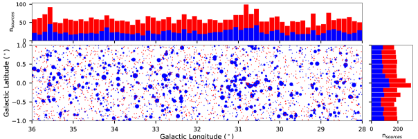
Figure 1: Spatial distribution of sources extracted from the VLA B-configuration images. Blue circles indicate the positions of highly reliable sources, their sizes are scaled (non-linear) with the flux intensity. Red points indicate the position of sources with 5 to 7$\sigma$ levels. Top and right panel are the histogram of the source distributions in the Galactic longitude and Galactic latitude, respectively.

The primary goal of the GLOSTAR survey is to localize signposts of massive star formation (MSF) activity (see Brunthaler et al., 2021, for a detailed overview of the survey). Towards this goal, in the continuum mode, the survey mainly observes compact, ultra- and hyper-compact HII regions, that trace different early phases of MSF activity (e.g., Medina et al., 2019; Nguyen et al., 2021). Thus, the GLOSTAR survey complements previous radio surveys by providing a powerful and comprehensive radio-wavelength survey of the ionized gas in the Galactic Plane with an unprecedented sensitivity. However, the survey area is also populated with radio sources related to post-main sequence stars (e.g. Wolf-Rayet stars, pulsars, etc.), planetary nebulae, supernova remnants and extragalactic radio sources (Medina et al., 2019; Chakraborty et al., 2020; Dokara et al., 2021). In spectral line mode, it traces the radio recombination lines from regions ionized by massive stars and the methanol maser line at 6.7 GHz (Ortiz-León et al., 2021; Nguyen et al., 2022), both of which are related to massive star formation. The formaldehyde absorption line at 4.8 GHz is also observed. It traces neutral molecular gas and its radial velocity information with respect to the local standard of rest (LSR) radial can help to solve distance ambiguities. The final GLOSTAR images will cover the Galactic plane between Galactic longitudes, $\ell$, of $-2^{\circ}$ and $60^{\circ}$ and latitudes, $b$, from $-1^{\circ}$ to $+1^{\circ}$ and the Cygnus X region. The final dataset will consist of low resolution images ($\sim 20^{\prime\prime}$), using the VLA in the D configuration, and high resolution images ($\sim 1\hbox to0.0pt{.\hss}^{\prime\prime}0$), using the B configuration. These VLA data sets could also be combined for optimal sensitivity of the intermediate spatial ranges, such images will be presented in future works. The VLA observations will be complemented with very low resolution ($\sim 150^{\prime\prime}$) images of single dish observations from the Effelsberg radio telescope, to recover the most extended emission and solve the “missing short spacing” issue affecting interferometer-only images. The overview of the full GLOSTAR capabilities are described in detail by Brunthaler et al. (2021).

Previously, we have reported the radio source catalog of the low resolution VLA images covering the area $28^{\circ}<\ell<36^{\circ}$ and $-1^{\circ}<b<+1^{\circ}$ (Medina et al., 2019). Complementary infrared- and sub-millimeter-wavelength data were examined towards the radio source positions with the goal to elucidate the nature of the radio sources. In this paper we report the compact ($\sim 1\hbox to0.0pt{.\hss}^{\prime\prime}0$) radio sources from the same region using the high resolution observations obtained with the VLA in B-configuration. The interesting part of this new catalog is that we can identify the most compact, and probably youngest, (hypercompact) HII regions.

2 Observations

The Karl G. Jansky Very Large Array (VLA) of the National Radio Astronomy Observatory was used in its B-configuration to observe the (4–8 GHz) continuum emission. We follow the same instrumental setups and calibration as for the D-configuration data. We refer the reader to the overview paper (Brunthaler et al., 2021) for a detailed description of the data management that we summarize in the following subsections.

2.1 Observation Strategy

The correlator setup consisted of two 1 GHz wide sub-bands, centered at 4.7 and 6.9 GHz. Each sub-band was divided into eight spectral windows of 128 MHz, and each spectral window comprising of 64 channels with a channel width of 2 MHz. The chosen setup avoids strong persistent radio frequency interference (RFI) seen (most prominently) at 6.3 and 4.1 GHz and allows estimation of source spectral indices.

For each epoch the total observing time was five hours. At the beginning of the observations, the amplitude/bandpass calibrator 3C 286 is observed for ten minutes. Then, the phase calibrator, J1804+0101, is observed for one minute, followed by pointings on target fields for eight minutes, after which the phase calibrator is observed for another minute. The observation cycle, consisting of phase calibrator–targets scans, is repeated over the full five hours. During this time, an area of $2^{\circ}\times 1^{\circ}$ is covered with phase centers for 676 target fields in a semi-mosaic mode (see Brunthaler et al., 2021, for a detailed overview of the observation strategy). Each pointing was observed twice for 11 seconds which, after considering the slewing time, yields a total integration time of 15 seconds per field. The theoretical noise level in brightness (or peak flux density) from these observations is 90 $\mu$Jy beam^-1 per field and per sub-band. The noise is improved after combining the fields and both sub-bands by a factor of $\sim 2$. We observed a total of eight epochs, or a total of 40 hours of telescope time, under project ID VLA/13A-334. The total covered area is 16 square degrees. The observations were taken during the period from 2013 September to 2014 January.

Table 1: GLOSTAR B-configuration catalog for $28\degr<\ell<36\degr$ and $|b|<1$°.

GLOSTAR B-conf.	$\ell$	$b$	SNR	$S_{\rm peak}$	$\bm{\sigma}_{\mathbf{S_{\rm peak}}}$	$S_{\rm int}$	$\mathbf{\bm{\sigma}_{S_{\rm int}}}$	$Y$	$R_{\rm eff}$	$\alpha$	GLOSTAR D-conf.	Infrared counterpart			Sub-mm	Classification
name	(°)	(°)		(mJy beam-1)		(mJy)			(″)		name	NIR	MIR	FIR	counterpart
(1)	(2)	(3)	(4)	(5)	(6)	(7)	(8)	(9)	(10)	(11)	(12)	(13)	(14)	(15)	(16)	(17)
G028.0014+00.0567	28.00144	+0.05670	15.6	0.90	0.08	0.86	0.07	0.95	0.8	$+0.28\pm 0.24$	G028.002+00.057					EgC
G028.0050+00.1497	28.00503	+0.14967	10.2	0.60	0.07	0.66	0.07	1.09	0.7	$-0.50\pm 0.60$	G028.005+00.150					EgC
G028.0065-00.9904	28.00648	-0.99038	35.6	2.49	0.15	2.48	0.14	1.00	0.9	$-0.24\pm 0.06$	G028.007-00.990	✓				EgC
G028.0101-00.3032	28.01014	-0.30323	12.6	0.69	0.07	0.72	0.07	1.04	0.8	$-0.11\pm 0.36$	G028.010-00.303					EgC
G028.0239+00.5132	28.02391	+0.51318	13.8	0.92	0.08	0.97	0.08	1.05	0.8	$+0.34\pm 0.35$	G028.024+00.514					EgC
G028.0309+00.6677	28.03085	+0.66769	08.2	0.54	0.07	0.62	0.07	1.13	0.7	…	G028.031+00.669		✓			EgC
G028.0314-00.0726	28.03136	-0.07260	31.9	2.03	0.13	2.44	0.14	1.20	1.0	$-0.79\pm 0.14$	…					EgC
G028.0350+00.3898	28.03495	+0.38978	10.2	0.69	0.08	0.70	0.08	1.01	0.7	$-0.59\pm 0.37$	…					EgC
G028.0403-00.2452	28.04027	-0.24519	09.2	0.56	0.07	0.52	0.07	0.94	0.7	…	…					EgC
G028.0474-00.9892	28.04741	-0.98918	23.2	1.86	0.13	2.10	0.13	1.13	0.9	$-0.33\pm 0.25$	G028.048-00.989					EgC
G028.0489-00.8699	28.04894	-0.86986	16.2	1.03	0.08	1.05	0.08	1.02	0.8	$+0.45\pm 0.25$	G028.049-00.869					EgC
G028.0594+00.1197	28.05937	+0.11975	11.5	0.84	0.09	0.84	0.08	1.00	0.7	$+0.36\pm 0.46$	G028.065+00.119					EgC
G028.0654+00.1184	28.06544	+0.11842	25.1	1.77	0.12	2.01	0.12	1.14	1.0	$-0.71\pm 0.26$	…					EgC
G028.0749-00.2953	28.07494	-0.29530	19.1	1.28	0.10	1.42	0.10	1.11	0.9	$-0.88\pm 0.27$	G028.075-00.296	✓				EgC
G028.0850-00.5583	28.08501	-0.55826	28.4	1.69	0.11	1.76	0.11	1.04	0.9	$-0.34\pm 0.16$	G028.085-00.558	✓				EgC

Notes: Only a small portion of the data is provided here, the full table is available in electronic form at the CDS via anonymous ftp to cdsarc.u-strasbg.fr (130.79.125.5) or via http://cdsweb.u-strasbg.fr/cgi-bin/qcat?J/A&A/.

Classification (17) see also section 3.8: EgC = Extragalctic radio source candidate, HII = HII region candidate, Radio-star, PN = planetary nebula, WR = Wolf-Rayet star, PDR = Photodissociation region, Cataclysmic variable, Pulsar, and Unclear = source with no clear classification.

Table 2: GLOSTAR D-configuration sources that are detected as fragmented sources (e.g., multiple components of an extended and resolved source) in the B-configuration images.

GLOSTAR B-conf.	GLOSTAR D-conf.	#	$S_{\rm int}$	Class
name	name	frag.	(mJy)
(1)	(2)	(3)	(4)	(5)
G028.2440+000.0143	G028.245+00.013	2	01.73	HII
G028.4518+000.0029	G028.451+00.003	3	12.98	HII
G028.6520+000.0278	G028.652+00.027	3	12.23	HII
G028.6871+000.1771	G028.688+00.177	2	10.48	HII
G029.9558-000.0167	W43 south-center	5	375.51	HII
G030.2529+000.0538	G030.253+00.053	3	06.31	HII
G030.9582+000.0868	G030.955+00.081	3	06.61	HII
G031.0695+000.0506	G031.069+00.050	2	09.11	HII
G031.2435-000.1103	G031.243-00.110	4	184.42	HII
G031.2797+000.0623	G031.279+00.063	4	10.15	HII
G031.4118+000.3064	G031.412+00.307	3	84.14	HII
G032.1501+000.1335	G032.151+00.133	5	27.41	HII
G032.2726-000.2257	G032.272-00.226	3	12.81	HII
G032.7965+000.1909	G032.798+00.191	2	574.36	HII
G032.9272+000.6060	G032.928+00.606	2	71.99	HII
G033.9145+000.1104	G033.914+00.110	3	106.65	HII
G034.1321+000.4720	G034.133+00.471	8	23.45	HII
G034.2571+000.1533	G034.260+00.125	3	733.11	HII
G034.8624-000.0630	G034.862-00.063	2	34.16	PN
G035.0521-000.5178	G035.052-00.518	2	08.62	HII
G035.4666+000.1393	G035.467+00.139	2	35.17	HII
G035.5641-000.4909	G035.564-00.492	4	07.93	PN

Notes: Column (1) gives the name of the brightest fragment.

2.2 Calibration, Data Reduction and Imaging

The data were calibrated, edited and imaged using the Obit software environment (Cotton, 2008), which inter-operates with the classic Astronomical Image Processing Software package (AIPS) (Greisen, 2003). We have written calibration scripts that handle the GLOSTAR data edition and calibration (Brunthaler et al., 2021). The calibration follows the standard procedures of editing and calibrating interferometric data. These include bandpass, amplitude and phase calibration.

The calibrated data were imaged using the Obit task MFImage. The CLEANing process from MFImage divides the observed band into nine frequency bins, that are narrow enough to perform a spectral deconvolution, addressing the effects of variable spectral index and antenna pattern variations. In the end, we obtained an image representing the data for the full frequency band and images of each individual frequency bin. The images were obtained from the data that had projected baselines with distances in the ${(u,\,v)}$-plane larger than 50 k$\lambda$; i.e., discarding all radio emission on angular scales larger than $\approx 4\hbox to0.0pt{.\hss}^{\prime\prime}13$ at all observed frequencies. This choice rejects emission from poorly mapped extended structures that introduced artifacts in the images, with a minor impact in the overall sensitivity. The images were convolved with a circular beam ${1\hbox to0.0pt{.\hss}^{\prime\prime}0}$ of size, and with pixel size of $0\hbox to0.0pt{.\hss}^{\prime\prime}25$. The mosaics are constructed to obtain images of ${35000\times 30000}$ pixels, containing the ${1^{\circ}\times 2^{\circ}}$ angular area surveyed by epoch, following the schemes described by Brunthaler et al. (2021). The mean measured noise in the resulting images is ${60\,\mu}$Jy beam^-1; though it can be significantly higher in some areas in which extended emission was not properly recovered or around very bright radio sources that produce imperfectly cleaned sidelobe emission.

3 Catalog construction

In this section we discuss the procedure used for constructing the catalogues presented in this work. First, we have extracted the sources from the images, selected the sources that are real, identified candidate radio sources, and discarded image artifacts. We have investigated the astrometry, flux density ($S_{\nu}$), spectral indices ($\alpha$; $S_{\nu}\propto\nu^{\alpha}$), and have searched for counterparts at other wavelengths. Based on the counterpart information, we attempted a classification of the radio sources. The final catalog is presented in Table 1, with the reliable radio sources, their properties and the source classification.

3.1 Source extraction

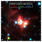
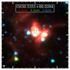
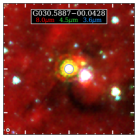
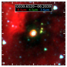
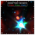
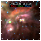
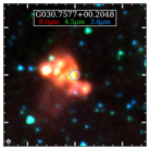
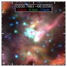
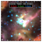
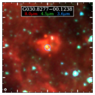
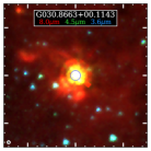
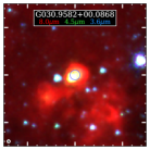
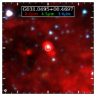
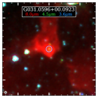
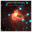
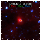
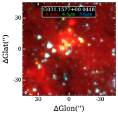
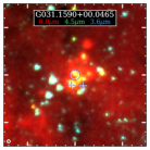
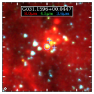
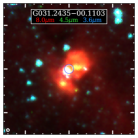
Figure 1: Continuation.

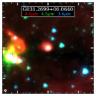
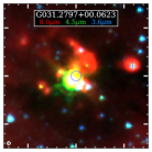
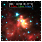
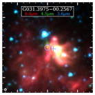
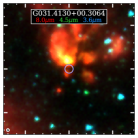
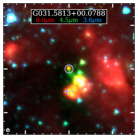
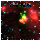
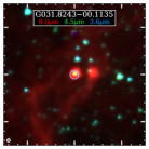
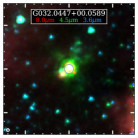
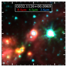
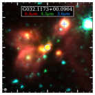
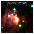
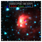
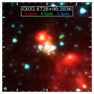
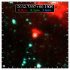
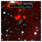
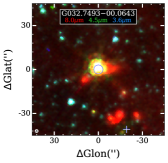
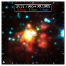
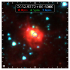
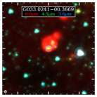
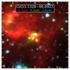
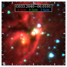
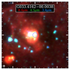
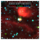
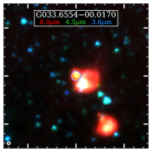
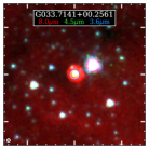
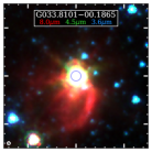
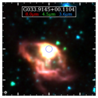
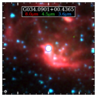
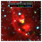
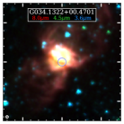
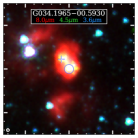
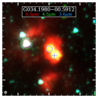
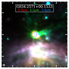
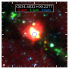
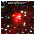
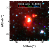
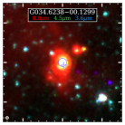
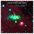
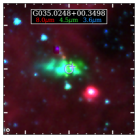
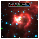
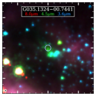
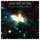
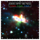
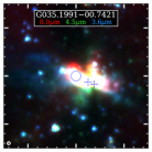
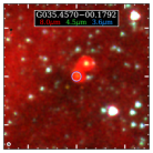
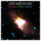
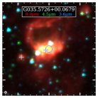
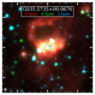
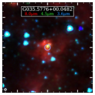
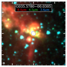
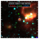
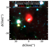
Figure 1: Continuation.

The source extraction was performed following the procedures described by Medina et al. (2019), and we refer the reader to that work for the details, while here we will give a brief summary. Using the SExtractor (Bertin & Arnouts, 1996) tool from the Graphical Astronomy and Image Analysis Tool package (GAIA), we first create a noise image. Then, we have used the BLOBCAT package (Hales et al., 2012) to extract the sources from each of the final images. Both the intensity map and the noise map are used as inputs by BLOBCAT. This package recognizes islands of pixels (blobs) representing sources with a minimum peak flux above $N$ times the noise level in the area. Purcell et al. (2013) noted that with $N<4.5$, large radio images will be dominated by spurious sources. Thus, to diminish the number of spurious detections in our catalog, for our extraction we have initially defined $N=5$ and require blobs to consist of a minimum of 12 contiguous pixels. The minimum number of pixels was chosen to be the number of expected pixels in 50% of the beam area. The final number of extracted blobs is 3880 . After this first extraction we performed a visual inspection of all the blobs to identify clear image artifacts, such as sidelobes from very bright radio sources, and discarded 555 blobs. The spatial distribution of all the blobs, excluding the artifacts, is shown in Figure 1. We detected a total of 1457blobs with a signal-to-noise ratio (S/N) $\geq 7.0$ and 1866  blobs with $5.0\leq{\rm S/N}<7.0$.

It has been determined that in large radio surveys such as GLOSTAR the most reliable sources are those with peak flux values above $7\sigma_{\rm noise}$ as no spurious sources are expected at these levels (e.g., Purcell et al., 2013; Bihr et al., 2016; Wang et al., 2018; Medina et al., 2019). However, as some blobs with a brightness between 5–7$\sigma_{\rm noise}$ could represent real sources, we have searched for counterparts inside a radius of $2^{\prime\prime}$ in the SIMBAD astronomical database for all sources (see details below). This comprehensive database is the best option to look for counterparts at any wavelength in large areas of the sky but, admittedly, it can miss recent catalogs. We have also considered weak blobs (peak flux values $<7\sigma_{\rm noise}$) as real radio sources whose positions are consistent with the radio sources from our D-configuration catalog by Medina et al. (2019). The full number of weak blobs with a known counterpart in the SIMBAD database and our D-configuration catalog is 142. The remaining 1724 radio blobs having a S/N between 5 and 7 and have no known counterpart are referred to as candidate radio source detections. We give the list of these 1866 sources with S/N$<7$ in Appendix A (Table 6) labeling those with SIMBAD or D-configuration counterparts, and we do not analyze them further.

We consider the remaining 1457 blobs as highly reliable radio sources. They are represented by the blue circles in Figure 1 and are listed in Table 1. The position, the SNR, the peak and the integrated flux density values (columns (2) to (8) in Table 1) are taken from the values determined by the BLOBCAT software (Hales et al., 2012). From now on, this paper will focus on the analysis of these sources. Considering the ratio between the integrated flux density (in units of Jy) and the peak flux density (in units of Jy beam^-1 (here named as the Y-factor; $Y=S_{\nu,{\rm Int}}/S_{\nu,{\rm Peak}}$) we can divide these sources into extended ($Y>2.0$), compact ($1.1<Y\leq 2.0$) and point-like ($Y\leq$1.1) sources. The $Y$ factor of each source is listed in column (9) of Table 1. Using this classification we obtain 100 extended, 455 compact, and 904 point-like sources. As expected for these images, the sources are dominated by compact and point-like sources as we have rejected extended structures in our imaging process.

3.2 Astrometry

For our previous catalog based on the VLA D-configuration observations we have estimated that the accuracy of the astrometry is of the order of $1^{\prime\prime}$. The position errors of the extracted sources with BLOBCAT in the VLA B-configuration images have a mean value of ${0\hbox to0.0pt{.\hss}^{\prime\prime}06}$ in both Galactic longitude and latitude. The ${0\hbox to0.0pt{.\hss}^{\prime\prime}06}$ is a formal statistical error estimate from BLOBCAT and does not reflect position errors resulting from imperfect phase calibration. As most of the observed radio sources are expected to be background extragalactic objects, the proper motion of these sources is expected to be zero. The only other recent Galactic plane survey that observed the same region at a similar radio frequency is the Co-Ordinated Radio ’N’ Infrared Survey for High-mass star formation (CORNISH; Hoare et al. 2012; Purcell et al. 2013). The observations of CORNISH were obtained at 5 GHz using the VLA in its B-configuration. Because of the similarity of the frequency and the use of the same VLA array configuration the angular resolution of CORNISH is ${1\hbox to0.0pt{.\hss}^{\prime\prime}5}$, similar as that of the GLOSTAR  survey B array data discussed here ($1\hbox to0.0pt{.\hss}^{\prime\prime}0$).

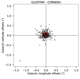
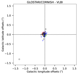
Figure 2: Upper panel: Position offsets between GLOSTAR compact and point-like sources ($Y\leq\,2$) and CORNISH sources. Filled red ellipse is centered in the mean values of the offsets and the size of the semi-axes are equal to the standard deviations. Lower panel: Similar as the top panel, but for position offsets of GLOSTAR (black crosses, red filled ellipse) and CORNISH (blue crosses, green filled ellipse) sources between the measured positions and the VLBI positions. Open black circles in the bottom-left of both panels indicate the mean of position errors of GLOSTAR-B sources.

A total of 257 compact and point-like sources are listed in both the GLOSTAR-B and CORNISH catalogs (Purcell et al., 2013) with a maximum angular separation of $1\hbox to0.0pt{.\hss}^{\prime\prime}5$, the CORNISH angular resolution. In the upper panel of Figure 2 the measured offsets of these sources are plotted. We obtain mean and standard deviation for the position offsets of ${-0\hbox to0.0pt{.\hss}^{\prime\prime}04\pm 0\hbox to0.0pt{.\hss}^{\prime\prime}01}$ and $0\hbox to0.0pt{.\hss}^{\prime\prime}17$ in Galactic longitude direction, and ${0\hbox to0.0pt{.\hss}^{\prime\prime}03\pm 0\hbox to0.0pt{.\hss}^{\prime\prime}01}$ and ${0\hbox to0.0pt{.\hss}^{\prime\prime}15}$ in Galactic latitude direction. The mean offsets in both directions are smaller than the mean position error of GLOSTAR radio sources, suggesting a good astrometry.

The most accurate positions of radio sources are obtained with the Very Long Baseline Interferometry (VLBI) technique. The Radio Fundamental catalog of extragalactic radio sources compiles the positions of $\sim 19,000$ sources that have been measured with VLBI. We found in this catalog 15 sources detected both by GLOSTAR and CORNISH. In the lower panel of Figure 2 we show the offsets between the GLOSTAR and the VLBI positions as black crosses, and the offsets between the CORNISH and VLBI positions as blue crosses. The mean GLOSTAR$-$VLBI position offset and its standard deviation is ${-0\hbox to0.0pt{.\hss}^{\prime\prime}05\pm 0\hbox to0.0pt{.\hss}^{\prime\prime}02}$ and $0\hbox to0.0pt{.\hss}^{\prime\prime}06$, respectively, in Galactic longitude direction, and $0\hbox to0.0pt{.\hss}^{\prime\prime}03\pm 0\hbox to0.0pt{.\hss}^{\prime\prime}03$ and $0\hbox to0.0pt{.\hss}^{\prime\prime}11$, respectively, in Galactic latitude direction. On the other hand, the mean CORNISH$-$VLBI position offset and its standard deviation is $-0\hbox to0.0pt{.\hss}^{\prime\prime}02\pm 0\hbox to0.0pt{.\hss}^{\prime\prime}02$ and $0\hbox to0.0pt{.\hss}^{\prime\prime}07$, respectively, in the Galactic longitude direction, and $-0\hbox to0.0pt{.\hss}^{\prime\prime}02\pm 0\hbox to0.0pt{.\hss}^{\prime\prime}03$ and $0\hbox to0.0pt{.\hss}^{\prime\prime}10$, respectively, in the Galactic latitude direction. The conclusion from this analysis is that the astrometry of the B-configuration GLOSTAR images presented in this paper is accurate to better than $0\hbox to0.0pt{.\hss}^{\prime\prime}1$.

3.3 Comparison with the D-configuration catalog

In the first GLOSTAR catalog, we have reported a total of 1575 discrete sources detected in the same region presented in this paper, but based on data obtained with the VLA in its most compact (D) configuration. The GLOSTAR images from the VLA D-configuration observations have an angular resolution of $18^{\prime\prime}$, i.e., 18 times larger than the VLA B-configuration images presented in this paper, which also excluded the shortest baselines to further filter out extended emission, resulting in some expected differences. First, given the higher angular resolution observations of the B-configuration, the extended radio sources reported by Medina et al. (2019) are resolved out and, in some cases, only the brightest peaks of extended sources are detected. It is worth noting that some compact sources detected in the B-configuration images can be seen projected on the area of the extended sources, although they do not represent their direct counterpart. Their possible relation must be studied further in future (e.g., upper-panel of Figure 3). Second, some multiple component radio sources that are unresolved or slightly resolved in the D-configuration images will be resolved in the B-configuration images (middle-panel of Figure 3) and the integrated flux densities of the individual components can be estimated. Third, some individual radio sources detected in the D-configuration images can be resolved and appear as fragmented radio sources in the B-configuration images (lower-panel of Figure 3). In total, we have found that 95 sources in the D-configuration images are resolved into 224 B-configuration sources (see column (12) of Table 1).

The components of fragmented radio sources are grouped and treated as a single source. However, the information of each single component is given in Table 1 and the fragmented sources are listed in Table 2. The integrated flux density reported in Table 2 is obtained by adding the integrated flux densities of the individual fragments. In total, 72 sources recovered from BLOBCAT are grouped into 22 fragmented sources.

Other sources were detected as single compact sources in both D- and B-configuration images and can be considered as direct counterparts. The mean position error of D-configuration sources is $1\hbox to0.0pt{.\hss}^{\prime\prime}2$ (Medina et al., 2019) and the beam size of the B-configuration images is ${1\hbox to0.0pt{.\hss}^{\prime\prime}0}$. Thus, by adding these values in quadrature we used a maximum angular separation of $2^{\prime\prime}$ between sources in both catalogs to consider them as direct counterparts. The number of matching sources between both catalogs with this criterion is 372. A further 312 matching sources are found using an angular separation of $9^{\prime\prime}$, half of the angular resolution of the D-configuration images, for which the association must be investigated further. Given the differences described above, the matching of sources between both catalogs is not expected to be one-to-one.

In column (12) of Table 1 we list the GLOSTAR D-configuration name to which the B-configuration source is related. With the D-configuration name we have also labeled those sources that are related to two or more B-configuration sources and if they are considered as individual (I) or fragmented (F) sources. In total, 908 B-configuration sources were related to 780 D-configuration sources. The remaining 551 B-configuration sources have no counterpart in the D-configuration catalog. Most of these sources are located in the inner parts of the Galactic plane (see Figure 4) where the noise level is higher in the D-configuration images because of the bright and extended radio sources (see the lower panel of Figure 1 in Medina et al., 2019). As the noise levels could be as high as $500\leavevmode\nobreak\ \mu$Jy beam^-1, it explains why most of the sources were not detected in the D-configuration images, but are detected in the B-configuration images where the noise level is about 10 times lower.

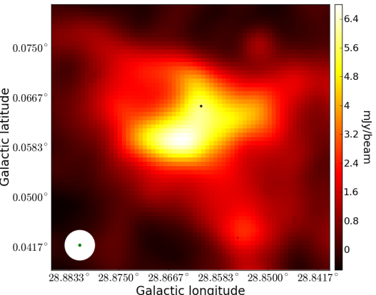
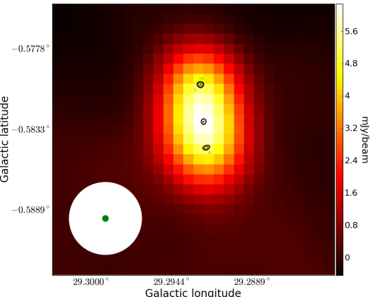
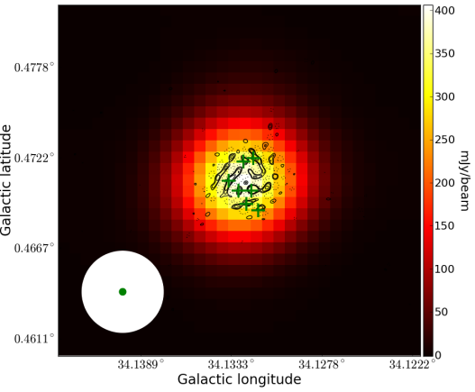
Figure 3: Source examples of the differences between the two sets of VLA images, D-configuration (background) and B-configuration (contours). Contour levels are $-5$, 5, 7, 10 and 15 times 60 $\mu$Jy beam^-1, the mean noise level of the images. Circles at the bottom-left side indicate the beam sizes of D-configuration ($18^{\prime\prime}$, white) and B-configuration ($1\hbox to0.0pt{.\hss}^{\prime\prime}5$, green) images. Top: B-configuration compact radio source seen in projection in the area of a D-configuration extended radio source. Middle: D-configuration compact source that is resolved in three individual compact radio sources in the B-configuration images. Bottom: D-configuration compact source that is resolved as a fragmented radio source. The position of fragments considered in the final catalog are indicated with green crosses.

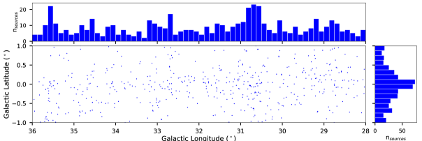
Figure 4: Spatial distribution of radio sources detected in the B-configuration images that have no counterparts in the D-configuration images.

3.4 Source sizes

The source sizes are obtained following Medina et al. (2019), who determined the source effective radius. BLOBCAT  determined the number of pixels comprising each source, which can be used to estimate the area ($A$) covered by the source using the pixel size of $0\hbox to0.0pt{.\hss}^{\prime\prime}25\times 0\hbox to0.0pt{.\hss}^{\prime\prime}25$. Then the effective radius can be determined using

$$R_{\rm eff}=\sqrt{\frac{A}{\pi}}.$$

The effective radius distribution is shown in Figure 5, and the value for each source is listed in column (10) of Table 1.

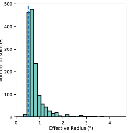
Figure 5: Distribution of the source effective radius. The dashed-dotted line indicates the resolution of the observations (half beam width). Note that the images are only sensitive to angular scales ${\leq 4\hbox to0.0pt{.\hss}^{\prime\prime}1}$. The bin size used is $0\hbox to0.0pt{.\hss}^{\prime\prime}15$.

3.5 Flux densities

To estimate the reliability of the radio source flux densities determined from the GLOSTAR images, we compare the results from the BLOBCAT extraction with those in the CORNISH catalog. As most of the sources are expected to be extragalactic sources whose variability is expected to be low (typically only of a few percent over timescales of several years) these provide a good point of comparison. We compare sources that are point like, and thus used the peak flux density. Moreover, we have only compared sources whose peak flux densities are above 2.7 mJy in both catalogs, as this is the 7$\sigma$ base point in the high reliability source catalog of CORNISH (Purcell et al., 2013). We found 207 sources that meet these criteria. A difference between both catalogs is the mean observed frequency. CORNISH observed at 5 GHz, and GLOSTAR observed a wider bandwidth centered at 5.8 GHz. The measured flux density thus is expected to differ slightly for this observational mismatch due to the spectral index. Assuming that the extragalactic objects have a mean spectral index of $-0.7$ (Condon, 1984), the CORNISH flux values will be on average 10% higher than in GLOSTAR.

In the upper panel of Figure 6 we plot the peak flux densities measured by the CORNISH survey as a function of the peak flux densities measured in this work. The dashed line indicates the equality line, and most of the sources are around this line. The lower panel of this figure shows the distribution of the peak flux density ratio between the results from both catalogs. A Gaussian fit to the distribution indicates that the mean value is ${1.11\pm 0.03}$ with a standard deviation of 1.28. Considering the expected higher values in the CORNISH catalog, we conclude that the integrated and peak flux densities of the GLOSTAR-B radio sources are accurate to within 10%.

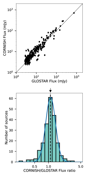
Figure 6: Upper panel: Comparison of the peak flux densities of radio sources detected in GLOSTAR-B and CORNISH. Lower panel: Histogram of the ratio between the peak flux densities of CORNISH and GLOSTAR. The width of the bars is 0.08 dex. The blue line indicates the model from the Gaussian fit to the histogram. The dashed line indicates the mean value of the distribution. The small arrow at the top of the plot show the expected CORNISH/GLOSTAR flux density ratio for the different observed mean frequency.

3.6 Spectral indices

The spectral index of a radio source gives us information on the dominant emission mechanism. Using the wide frequency coverage of our observations we can estimate the spectral index within the observed band. We measure the peak flux density in each of the imaged frequency bins for compact and point like sources that have S/N$>10$ in our main source extraction, a total of 988 sources. The constraint of the S/N was chosen to consider that the noise level in each of the imaged frequency bins will be $\sim 3\times$ higher, and may thus not be detected in the individual frequency bin images or their determined values will be affected by noise. On the other hand, over the area covered by an extended source, flux density variations that will depend on its structure may be observed at each frequency, and are hence not considered for this analysis. To obtain the spectral index we assume that in the observed frequency range the flux density is described by the linear equation:

$${\log{S_{\nu}}=\alpha\cdot\log{\nu}+C}.$$

A weighted least-square fitting is made to the measured flux densities. Independent spectral index values for each source are listed in column (11) in Table 1. The distribution of the determined spectral indices is shown in Figure 7. The distribution of spectral indices has a mean value of $-0.66\pm 0.02$.

Spectral indices at radio frequencies in the same area of the presented images have been measured previously from the GLOSTAR D-configuration (Medina et al., 2019) and in the THOR survey (Bihr et al., 2016, ; described in the next section). To compare the different results, we have selected the sources that have spectral indices determined and have point like structure ($Y\leq 1.1$) in all three sets of results. The last constraint is imposed to diminish effects of possible scale structure differences as GLOSTAR D-configuration and THOR have angular resolutions of $18^{\prime\prime}$. Figure 8 shows the histogram distributions of the spectral index differences of the three sets. We found that the measured spectral indices are consistent among the three data sets, given that the mean of the differences is consistent with zero. We thus conclude that the spectral indices measured on GLOSTAR B-configuration images are reliable.

In star forming regions, three main mechanisms are known to produce compact radio continuum emission, and are related to different astrophysical phenomena (Rodríguez et al., 2012). The majority of radio sources show thermal free-free radio from ionized gas (e.g., HII regions, externally ionized globules, proplyds, jets) that has a spectral index ranging from $2.0$ (optically thick) at low frequencies to $-0.1$ (optically thin) at high frequencies. Magnetically active low-mass stars, may show nonthermal gyrosynchrotron with spectral indices ranging from $-2.0$ to $+2.0$. Nonthermal synchrotron emission arising from colliding winds in high mass binaries as well from jets ejected by high mass stars interacting with the ambient interstellar medium (ISM) have a typical spectral index of $-0.7$. However, other phenomena not related to star formation also can produce thermal radio emission, namely gas ionized in planetary nebulae (PNe), while synchrotron emission is observed from extragalactic sources. Background active galactic nuclei (AGN) will mostly emit optically thin synchrotron emission with spectral indices $\sim-0.7$. On the other hand, a fraction (up to 20%) of extragalactic background radio sources show a flat or positive spectral indices (e.g., Callingham et al., 2017). These represent a population of star forming galaxies, and progenitors of AGNs (i.e., high frequency peakers Dallacasa et al., 2000; Dallacasa, 2003). Given the diversity of the radio sources, to better understand their nature, information at other wavelengths is required. This will be discussed in the following subsection.

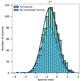
Figure 7: Distribution of the in-band determined spectral indices. Blue dotted bars show the spectral index distribution of sources with no counterparts at any other wavelength.

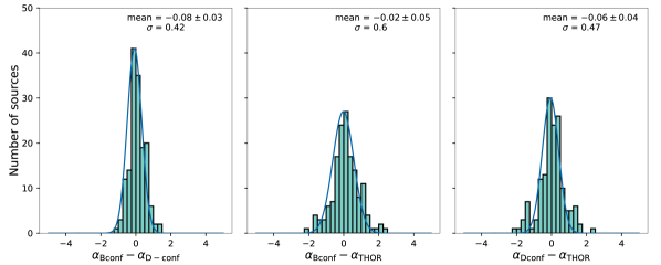
Figure 8: Spectral index difference distributions. From left to right: GLOSTAR B-configuration and GLOSTAR D-configuration, GLOSTAR B-configuration and THOR, and GLOSTAR D-configuration and THOR.

3.7 Counterparts at other wavelengths

To gain more insight on the nature of the radio sources, we have searched for counterparts at shorter wavelengths. The search was focused on catalogs that could give us evidence for ionized gas, dense cold gas and dust, which are indicators of massive young stars and the regions they form in. We now briefly describe the catalogs used in our search.

The APEX Telescope Large Area Survey of the Galaxy (ATLASGAL) observed the galactic plane at a wavelength of 870 $\mu$m (345 GHz), and angular resolution $\sim 20^{\prime\prime}$ (Schuller et al., 2009). The emission at this wavelength is dominated by dense cool gas and dust. Several ATLASGAL source catalogs have been released by Contreras et al. (2013), Csengeri et al. (2014), and Urquhart et al. (2014), who list $>10,000$ dense clumps. We will compare our results with the compact source catalog presented by Urquhart et al. (2014). The differences between the angular resolution of ATLASGAL and the observations presented here have to be taken into account. Thus, we have used an offset of $18^{\prime\prime}$ (roughly the beam size of ATLASGAL images) to consider an ATLASGAL source to be a potential counterpart for the compact radio source. We found 143 radio sources matching the position of 83 submillimeter sources.

The Herschel infrared Galactic plane survey (Hi-GAL) observed the inner Galaxy in 5 bands distributed in the wavelength range between 70 $\mu$m and 500 $\mu$m (Molinari et al., 2010, 2016). Notably, data taken at these wavelengths allow determinations of the peak of the spectral energy distribution of cold dust and thus the source temperatures. The Hi-GAL observations have angular resolutions from $10^{\prime\prime}$ down to $35^{\prime\prime}$ from the shortest to the longest wavelength. The median uncertainty of Hi-GAL sources is $\sim 1\hbox to0.0pt{.\hss}^{\prime\prime}2$. We have used a $2^{\prime\prime}$ offset between a Hi-GAL source and a GLOSTAR source to consider them as counterparts, and found 98 sources that matched this criterion.

The Wide-field Infrared Survey Explorer (WISE) mapped the entire sky in four infrared bands centered at 3.4, 4.6, 12.0, and 22.0 $\mu$m. The WISE ALL-sky Release Source Catalog contains astrometry and photometry for over half a billion objects (Wright et al., 2010). The angular resolution of the observations is $6^{\prime\prime}$ at the shortest wavelength and the position errors are around $0\hbox to0.0pt{.\hss}^{\prime\prime}2$. To consider a WISE source as the counterpart to a GLOSTAR radio source we have used a maximum offset of $2^{\prime\prime}$. A total of 125 sources match this criterion.

The Galactic Legacy Infrared Mid-Plane Survey Extraordinaire (GLIMPSE; Benjamin et al., 2003; Churchwell et al., 2009) mapped a large fraction of the Galactic plane with the Spitzer space telescope. It observed in four near-infrared sub-bands covering the range from 3.6 to 8.0 $\mu$m, and with angular resolutions $\sim 2^{\prime\prime}$. While the filter widths of the 3.6 and 4.5 $\mu$m bands are similar to those of WISE, the GLIMPSE survey has focused on Galactic plane observations and is more sensitive than the former. The interstellar medium emission at these wavelengths comes mainly from warm and dusty embedded sources. Considering the angular resolution of our observations and the position uncertainties in the GLIMPSE survey we have used an offset of $2^{\prime\prime}$ for the counterpart searching, leading to 251 matching sources.

The United Kingdom Infrared Deep Sky Survey (UKIDSS) is a suite of five public surveys at near infrared wavelengths (NIR) of varying depth and area coverage (Lucas et al., 2008). Particularly, the UKIDSS Galactic plane survey (UKIDS-GPS) covered a total of 1878 deg² of the northern hemisphere Galactic plane. The main observed bands are the so called J (1.25$\,\mu$m), H (1.65$\,\mu$m) and K (2.20$\,\mu$m) bands. The spatial resolution of UKIDSS-GPS observation is typically better than $0\hbox to0.0pt{.\hss}^{\prime\prime}8$. For the counterpart search of GLOSTAR radio sources in the UKIDSS-GPS catalog we have used this value of $0\hbox to0.0pt{.\hss}^{\prime\prime}8$, finding 389 matches.

After our careful search of counterparts at other wavelengths, it is noticeable that 640 radio sources have no counterparts at any other wavelength. The spectral index distribution of the sources in this category shows that they have preferably negative spectral indices (see Fig 7). We will further discuss these sources in the next section.

3.8 Classification of radio sources

Using the counterparts of the radio sources in the catalogues described in the previous section, a robust classification can be carried out. A single classification was performed for fragmented sources listed in Table 2 instead of separate classifications of their fragments, and thus the classification was done to 1409 sources. The classification criteria are based on our findings of the emission properties and/or counterparts of near-infrared (NIR; UKIDSS), mid-infrared (MIR; GLIMPSE and WISE), far-infrared (FIR; Hi-Gal), and submillimeter (SMM; ATLASGAL).

Images from the above mentioned infrared surveys are plotted at the position of the radio sources, some examples can be seen in Appendix B. For SMM and FIR, we show the emission properties of each GLOSTAR source. For NIR and MIR, we did a visual inspection of the three-color images for the UKIDSS (red K-band, green H-band and blue J-band), the GLIMPSE (red 8.0 $\mu$m, green 4.5 $\mu$m, and blue 3.6 $\mu$m), and the WISE (red 22.0 $\mu$m, green 12.0 $\mu$m and blue 4.6 $\mu$m) surveys. The sources have been classified into 5 groups, using the following criteria:

• HII region candidates: Radio sources with emission at SMM and FIR wavelengths and with weak or no emission at MIR and NIR (Hoare et al., 2012; Anderson et al., 2012; Urquhart et al., 2013; Yang et al., 2021).

• Radio star: Compact radio sources showing blue compact emission in the three color images of NIR and MIR wavelengths. Weak or no emission at FIR wavelenghts and no-emission at SMM wavelengths (Hoare et al., 2012; Lucas et al., 2008).

• Planetary nebula (PN): Show red emission in the three color images of NIR and MIR wavelengths where it is also seen as an isolated point source. Weak or no emission at far infrared (FIR) and submillimeter (SMM) wavelengths (Hoare et al., 2012; Anderson et al., 2012; Phillips & Marquez-Lugo, 2011).

• Photo dissociated region (PDR): Ionized gas seen as extended emission at MIR, and showing only weak or no compact emission at FIR and SMM wavelengths (Hoare et al., 2012).

• Extragalactic candidate (EgC): Radio sources that have no-counterpart at any other wavelength, or are only seen as a point source at NIR wavelengths (Hoare et al., 2012; Lucas et al., 2008; Marleau et al., 2008).

• Other sources. Sources that could not be classified in any of the previous categories.

The number of radio sources in these groups are 93 HII region candidates, 4 PDRs, 83 radio stars, 65 PNs, 1163 EgCs, and 2 other sources. Examples of sources in these classes are shown in Figures 11, 12, 13, and 14. The individual source classification is given in column (17) in Table 1 and in column (5) of Table 2 for fragmented sources.

3.9 Sources previously classified

Classification of the radio sources is a main part of the catalog construction. However, some of the sources could have been previously classified. A search for previous classifications of the radio sources has been performed using the SIMBAD astronomical database (Wenger et al., 2000), within a radius of $2^{\prime\prime}$. We found that 269 radio sources have counterparts in the SIMBAD database. Most of these sources, 138, are only classified as radio sources, and are thus of an unknown nature. The classification of the remaining 107 sources suggests that these are Galactic sources. In Table 3 we have separated these sources in seven types of sources, and have listed the source class in SIMBAD considered for these types and the number of sources of each type.

Table 3: Source classification from SIMBAD database.

Type	SIMBAD classa	#
Evolved stars	WR*, PN, PN?, AB?, CV*	38
Pulsars	Psr	3
Stars	*, Cl*	7
Young stellar objects	Y*O, Y*?	30
HII regions	HII	28
Gamma-Ray source	gam	1
Extragalactic objects	QSO	1
Other objects	Mas, mm, smm, IR, NIR, MIR, MoC, EmO, PoC, cor	23

^a The SIMBAD object classification is described in
http://simbad.u-strasbg.fr/simbad/sim-display?data=otypes.

4 Discussion

4.1 Overview of the final classification

The final radio source classification is a combination of the method described in Section 3.8, and the use of known information of individual sources recovered from the SIMBAD database. For our final catalog we additionally consider the SIMBAD classification for sources for which we find no counterpart in the searched IR and sub-mm catalogs. This was, for example, the case for pulsars that are usually not detected at infrared wavelength and are non-thermal radio emitters. Based on the criteria described in the previous section they were first classified as EgCs and after consulting the SIMBAD database they were finally classified as pulsars. A similar situation occurred with a Wolf-Rayet star and a cataclysmic variable star, wherein they were initially classified as a PN and as a Radio-star, respectively. We use the classification recovered from SIMBAD in these cases.

In Table 4 we give the number of sources found in each of the classifications. Interesting sources are the HII region candidates, as they are related to massive star formation, that we will discuss later.

Table 4: Final source classification of radio sources.

Classification	#
HII region candidates	93
WR	2
Pulsar	3
Radio stars	81
PNe	64
Cataclysmic Variable	1
PDRs	4
Other	2
EgCs	1157

4.2 Comparison of classifications

Classifications of some of the detected radio sources have been performed in previous radio surveys and here we will compare the results of these classifications. We will focus on a comparison based on the low resolution GLOSTAR D-configuration image presented by Medina et al. (2019), and with the classification based on the CORNISH survey which has a similar angular resolution observation as our B-configuration data (Purcell et al., 2013).

4.2.1 GLOSTAR D-configuration

Some differences between the present catalog and that derived from the D-configuration data are expected, since for the latter, the search for counterparts was done using larger angular separations than in this work on account of the lower resolution. 54 of the HII region candidates identified by us were also detected in D-configuration images, and were also identified as HII regions. Four other HII region candidates had a D-configuration counterpart, but were unclassified. The remaining 32 HII region candidates were not detected in the D-configuration images. Additionally, six sources classified as HII region candidates in the D-configuration catalog have been classified as PNe in the present work as their positions are no longer coincident with ATLASGAL sources.

We have detected 32 radio sources that were classified as PNe in the D-configuration catalog, of which 30 are classified as PNe in this work, one is classified as a WR star and another as an EgC because it is no longer positionally coincident with IR emission. We also detect 13 sources identified as radio stars in the D-configuration, of which 10 were related to a radio source also classified as radio stars. The remaining source, G028.098–00.781, was resolved into three different sources, two of them were classified as extragalactic sources and the other as PN. A further 749 sources detected in D-configuration images were also detected in the B-configuration images. Among these, 688 were classified as EgCs, consistent with the suggestion by Medina et al. (2019) that most of their unclassified radio sources are background extragalactic radio sources. The remaining 61 unclassified sources in D-configuration have now been classified, 43 as radio-stars, 14 as PNe, and 4 as HII region candidates. A comparison between the method used in the D-configuration data and in the B-configuration data shows a consistency better than 90% in the resulting classes.

4.2.2 CORNISH Survey

The CORNISH survey has a similar angular resolution, and it also used IR information to classify detected radio sources. In their classification effort, they consider UCHII regions and dark HII regions; we detected radio emission from 40 CORNISH sources classified as UCHII and from one dark HII region, which are classified as HII region candidates by us. We also have detected 25 CORNISH radio sources classified as PNe, that are also classified as PNe in our work. Seventeen radio-stars in the CORNISH survey have counterparts in our catalog; we classified fifteen of them also as radio-stars and two of them as EgCs because we did not find IR counterparts. We have detected 171 CORNISH radio sources classified as IR-Quiet (not detected at IR wavelengths); we classify 167 of them as EgCs, 4 as radio-stars as IR emission is now reported in the position of these sources, and one as a pulsar based on the SIMBAD database. Finally, out of the 29 radio-Galaxy sources in CORNISH, 28 are classified as EgCs in our work, and the remaining source is classified as radio-star given its IR properties. The consistency in classification between CORNISH and GLOSTAR B-configuration is high, especially for HII regions and PNe where we found a 100% agreement.

4.2.3 THOR survey

The HI/OH/Recombination line survey of the Milky Way (THOR; Bihr et al., 2015; Beuther et al., 2016; Wang et al., 2020) observed the northern hemisphere of the Galactic plane with the VLA in C-configuration and using its L-band receivers (1 to 2 GHz). It covers Galactic longitudes from 14.^∘5 to 67.^∘4 and Galactic latitudes from $-1\hbox to0.0pt{.\hss}^{\circ}$25 to 1.^∘25, i.e., including the area of the maps presented in this paper. The angular resolution of the THOR radio continuum images is $25^{\prime\prime}$ and they have noise levels from 0.3 to 1.0 mJy beam^-1 (Wang et al., 2018). While a detailed comparison of the source classification by THOR and GLOSTAR B-configuration is limited given the different image angular scales, it is still, however, useful.

To compare GLOSTAR B-configuration sources with THOR sources, we used a maximum separation of $2\hbox to0.0pt{.\hss}^{\prime\prime}5$, which is the position accuracy of the THOR survey (Wang et al., 2018). We found 554 sources matching in position between these surveys. From these sources, the THOR survey identified 34 HII regions (26 of which are identified as HII region candidates) and 9 as PNe (also identified as PNe with our classification criteria). Our classification for the remaining eight sources identified as HII regions by the THOR survey is four EgCs and four PNe. Differences between the classification of these sources can be caused by the different angular scales used for comparison with IR surveys. In fact, the median match radius of IR HII regions (identified with the WISE survey; Anderson et al., 2014) with the THOR survey is $\sim 60^{\prime\prime}$ (Wang et al., 2018), almost two orders of magnitude larger than our angular resolution.

4.3 HII region candidates

We have identified 93 HII region candidates. Out of these sources, 71 were previously related to HII regions from our analysis of the D-configuration images or from CORNISH or from THOR or from the SIMBAD database and 22 are new detections from this work. A characteristic of the radio emission from HII regions is that the spectral index values ranges from $-0.1$ (optically thin free-free radio emission) to 2.0 (optically thick free-free radio emission). Observationally, the spectral index distribution of hundreds of young HII regions at similar frequencies show a mean value of 0.6 (Yang et al., 2019, 2021). We have determined the in-band spectral index (see Section 3.6) for 57 HII region candidates, 13 of which are new. In Figure 9, we plot the spectral index of these HII regions as a function of the $R_{\rm eff.}$ the Y-factor and the S/N. Surprisingly, some of the determined spectral indices are negative and well below the lowest value expected for free-free radio emission of $\alpha=-0.1$, indicating that the radio emission nature is non-thermal. The results are not affected by the size of the source, as most of them are slightly resolved sources ($R_{\rm eff}\simeq\theta_{resolution}/2={0\hbox to0.0pt{.\hss}^{\prime\prime}50}$).

Kalcheva et al. (2018) obtained the spectral index to known ultra-compact HII regions and found that about 18% of their sample were consistent with negative spectral indices. They discuss their results and conclude that different interferometer array configurations and time variability could explain these negative values. These effects, however, are not present in the GLOSTAR observations presented here. Hence, these radio sources with negative spectral indices could be related to HII regions but they are not the HII regions themselves (e.g. Purser et al., 2016).

Compact radio sources have been found related to HII regions. The most known and nearby case is the Orion Nebula Cluster (ONC) where around 600 compact radio sources are found in the HII region ionized by the Trapezium (Forbrich et al., 2016; Vargas-González et al., 2021). As first suggested by Garay et al. (1987); Garay (1987), most of these fall into two broad categories: first, sources with thermal radio emission from circumstellar matter, often protoplanetary disks (“Proplyds”), that are photo-evaporated in the intense UV field of the brightest Trapezium star $\theta^{1}$ Ori C (O7Vp). Second, nonthermal sources associated with the coronal activity of magnetically active low mass members of the ONC many of which also show X-ray emission and are (highly) variable (Forbrich et al., 2021; Dzib et al., 2021). Other example regions are NGC 6334 (Medina et al., 2018) and the M17 (Rodríguez et al., 2012) star forming regions (SFRs) where several radio sources are found close to prominent HII regions. Also, in these SFRs a significant fraction of the compact radio sources have been found to produce non-thermal emission. That high number of such radio sources can be detected on the ONC is a result of the cluster’s close distance, $D$, of just $\approx 400$ pc (Menten et al., 2007; Kounkel et al., 2017). Extrapolating the Orion case to a distance of a few kilo-parsecs, most of these magnetically active stars would not be detected, except for the two strongest sources with measured integrated flux densities of a few tens of mJy. We note that, NGC 6334 and M17, mentioned above, are also relatively nearby, at $D$ = 1.34${}^{+0.15}_{-0.12}$ and $1.98_{-0.12}^{+0.14}$ kpc, respectively (Reid et al., 2014; Wu et al., 2014). Time variable weak radio sources around the well-studied ultracompact HII region W3(OH) ($D=2.0$ kpc) are other examples (Wilner et al., 1999).

For more distant SFRs, thermal radio emission is only detected from the HII region itself that is excited by the central high mass star(s) of a cluster.

It should be noted that other phenomena can produce compact non-thermal radio emission in massive star forming regions that are at work in Orion and can be observed in regions at distances of a few kpc, such as non-thermal radio jets (e.g. Carrasco-González et al., 2010; Purser et al., 2016) and wind collision regions in massive binary stars (e.g. Dzib et al., 2013). Non-thermal radio jets from YSOs, however, are rare and only a handful of cases are known. Similarly, non-thermal radio emission from wind collision regions are not common and are usually associated with evolved massive stars that have powerful winds.

On the other hand, the radio sources with positive spectral index could be true HII regions. More extensive multi-wavelength radio analysis is needed to characterize their emission and determine their turnover frequency, emission measure, etc. In general, all the radio sources that are associated with HII regions discussed in this work deserve further attention and more detailed studies.

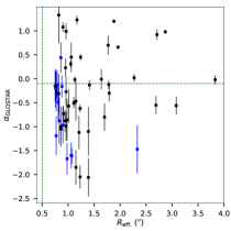
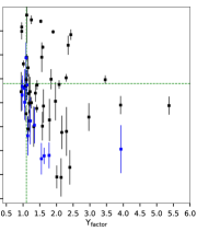
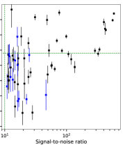
Figure 9: Spectral index of identified HII region candidates as a function of the effective radius (left), Y-factor (center) and S/N (right). Black symbols are sources that are related to previously identified HII regions, and blue symbols are the new identified HII region candidates.

4.4 Variable radio sources

By comparing the peak flux densities measured in the GLOSTAR images with those reported in CORNISH (Purcell et al., 2013), we have looked for sources with variable radio emission. The search was restricted to sources with $Y<2.0$, i.e., with compact radio emission. Variability is identified when the source is detected in both catalogs, GLOSTAR and CORNISH, but the flux ratio is larger than 2.0. We also identify variability when we detect a source in the GLOSTAR catalog with a peak flux density level $>2.7$ mJy beam^-1 (the CORNISH detection limit) and it is not reported in the CORNISH catalog. Finally, a source detected as unresolved in the CORNISH catalog that is not in the GLOSTAR high reliability catalog or in the catalog of sources with 5 to 7$\sigma$, is also considered as a variable radio source.

Table 5: Variable radio sources.

	GLOSTAR			CORNISH
Source	$S_{\rm peak}$	$\bm{\sigma}_{\mathbf{S_{\rm peak}}}$		$S_{\rm peak}$	$\bm{\sigma}_{\mathbf{S_{\rm peak}}}$
name	(mJy beam-1)		Classification	(mJy beam-1)		Classification
(1)	(2)	(3)	(4)	(5)	(6)	(7)
G028.1875+00.5047	…	…	…	2.61	0.39	IR-Quiet
G028.3660–00.9640	…	…	…	2.92	0.48	IR-Quiet
G028.4012+00.4776	…	…	…	5.25	0.60	Radio-Galaxy
G028.6043–00.6530	2.79	0.17	EgC	…	…	…
G028.9064+00.2548	…	…	…	3.47	0.53	IR-Quiet
G028.9224–00.6589	5.07	0.29	EgC	…	…	…
G029.1640–00.7922	3.05	0.18	EgC	…	…	…
G029.2620+00.2916	…	…	…	2.76	0.45	IR-Quiet
G029.3096+00.5124	…	…	…	2.84	0.43	IR-Quiet
G029.4302–00.9967	…	…	…	2.83	0.48	IR-Quiet
G029.4404–00.3199	…	…	…	2.81	0.47	IR-Quiet
G029.4959–00.3000	5.43	0.30	EgC	…	…	…
G029.5184+00.9478	…	…	…	2.43	0.40	IR-Quiet
G029.5780–00.2686	12.31	0.69	PN	6.22	0.72	PN
G029.5893+00.5789	1.73	0.12	EgC	4.17	0.50	IR-Quiet
G030.2193+00.6501	…	…	…	2.80	0.42	IR-Quiet
G030.3704+00.4824	2.83	0.16	HII	…	…	…
G030.6328–00.7232	…	…	…	2.57	0.40	IR-Quiet
G030.6517–00.0605	3.08	0.21	PN	…	…	…
G030.7859–00.0298	3.72	0.35	Other	…	…	…
G030.9704–00.7436	…	…	…	2.47	0.38	IR-Quiet
G031.0025–00.6330	2.78	0.17	EgC	…	…	…
G031.0450–00.0949	…	…	…	2.63	0.40	IR-Quiet
G031.0777+00.1703	13.37	0.74	EgC	6.75	0.72	IR-Quiet
G031.2989–00.4929	3.43	0.21	Radio-star	…	…	…
G031.3444–00.4625	…	…	…	2.78	0.37	IR-Quiet
G031.3917+01.0265	…	…	…	2.39	0.38	Radio-Star
G031.3993–00.0813	5.31	0.30	EgC	…	…	…
G031.5694+00.6870	26.11	1.44	EgC	6.79	0.71	IR-Quiet
G031.9943+00.5156	3.14	0.18	EgC	…	…	…
G032.2739–00.0358	2.91	0.17	EgC	…	…	…
G032.3843–00.3397	3.95	0.23	EgC	…	…	…
G032.4536+00.3679	1.42	0.10	EgC	2.74	0.46	IR-Quiet
G032.5898–00.4469	3.14	0.18	EgC	…	…	…
G032.5996+00.8265	2.87	0.17	EgC	5.92	0.62	IR-Quiet
G032.7396+00.8344	2.78	0.16	EgC	…	…	…
G032.7568+00.0959	2.76	0.18	EgC	…	…	…
G033.1860+00.9528	2.86	0.17	EgC	…	…	…
G033.3513+00.4056	…	…	…	2.62	0.40	IR-Quiet
G033.4100–00.4775	3.05	0.18	EgC	…	…	…
G033.4584+00.0163	3.82	0.22	EgC	…	…	…
G033.8964+00.3251	2.87	0.17	Radio-star	…	…	…
G033.9622–00.4966	…	…	…	2.81	0.42	IR-Quiet
G034.2171–00.6886	…	…	…	2.16	0.34	IR-Quiet
G034.4794–00.1683	2.78	0.16	EgC	…	…	…
G034.7242+00.6660	2.8	0.17	EgC	…	…	…
G035.0605+00.6208	…	…	…	2.76	0.43	IR-Quiet
G035.2618+00.1079	…	…	…	2.36	0.39	IR-Quiet
G035.9038–00.4810	2.26	0.14	EgC	4.94	0.55	IR-Quiet

Notes: Names for sources not detected in GLOSTAR images come from the CORNISH catalog (Purcell et al., 2013).

With the above criteria we have identified 49 variable sources. They are listed in Table 5 together with the peak flux densities in the compared catalogs. The GLOSTAR and CORNISH classification are listed when available. Most of the identified variable radio sources are EgC or IR-quiet sources, and have only been detected at radio wavelengths. Since extragalactic background sources are not expected in general to show pronounced variability, thus some of these sources could be interesting Galactic radio sources whose nature has to be explored.

4.5 Extragalactic Objects

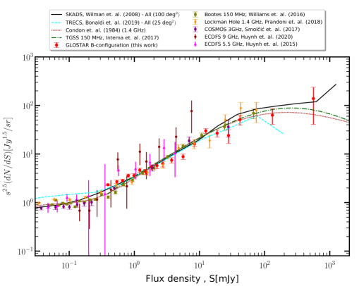
Figure 10: The Euclidean-normalized differential source counts of the point sources classified as of extragalatic origin in the GLOSTAR survey. We have compared the source counts with the simulated radio sky and previously observed source populations. For details of simulated catalogues and different observed source populations see text.

As has been shown in our previous works, most of the detected radio sources are expected to be background extragalactic objects (Medina et al., 2019; Chakraborty et al., 2020). Following the formulation by Fomalont et al. (1991), and using an observed area of 57,600 arcmin², assuming a nominal noise level of $\sigma=\,$65 $\mu$Jy beam^-1 and a threshold 7$\times$ the noise level, we estimate that the number of expected background extragalactic sources in our image is $1138\pm 664$. This number suggests that most of the detected radio sources above $455\,\mu$Jy beam^-1 (7$\sigma$) are of extragalactic origin.

From our classification criteria we have compiled a list of 1159 sources that have most probably an extragalactic origin. They are labeled as EgC in Table 1. Their extragalactic nature is also supported with the negative spectral index of most of them. The spectral index is determined for 777 of these sources and 157 (20%) have a flat or positive spectral index, consistent with the expected number of extragalactic radio objects that are expected to have positive spectral indices at our frequencies.

Similar to our previous work (Chakraborty et al., 2020), we have also studied the Euclidean-normalized differential source counts of the point sources characterized as being extragalactic in origin. We have binned the source integrated flux densities in logarithmic space and divided the raw counts in each bin by the fraction of image area over which a source with a given integrated flux density value can be detected, known as the visibility area (Windhorst et al., 1985). The differential source counts have been calculated by dividing the visibility area weighted source counts in each bin, by the total image area ($\Omega$ in steradians) and bin width ($\Delta S$ in Jy). These differential source counts have been normalized by multiplying with $S^{2.5}$, where $S$ is the mean integrated flux density of sources in each bin (Windhorst et al., 1985). The normalized differential source counts is shown in Figure 10, where the error bars are Poissonian. We have compared our findings with two simulated catalogues, the SKA Design Study simulations (SKADS, Wilman et al. 2008) and the Tiered Radio Extragalactic Continuum Simulations (T-RECS, Bonaldi et al. 2019). We have also compared our findings with the observed extragalactic source populations at low-frequency as well as high-frequency, which include: the TIFR GMRT Sky Survey at 150 MHz (TGSS-ADR1; Intema et al. (2017)), BOOTES field at 150 MHz using LOFAR (Williams et al., 2016), Lockman Hole field at 1.4 GHz with the LOFAR (Prandoni et al., 2018), COSMOS field at 3 GHz with VLA (Smolčić et al., 2017), ECDFS field at 5 GHz (Huynh et al., 2015) and 9 GHz (Huynh et al., 2020) with ATCA and the 1.4 GHz source counts based on observations with VLA by Condon (1984). In all cases we have scaled the source counts to 5.8 GHz using a spectral index, $\alpha=-0.7$. We have found that the source count of these sources classified as extragalactic in the GLOSTAR survey is statistically similar and consistent with the previously observed extragalactic source population as well as with the simulated catalogs. This shows that the majority of these sources are indeed of extragalactic origin.

4.6 Perspective on the search of non-thermal galactic sources

Figure 7 shows that the peak of the spectral index distribution is ${-0.66\pm 0.02}$. As discussed in the previous subsection most of the unidentified radio sources will be of extragalactic origin, however some of these will be interesting Galactic non-thermal radio sources. These sources are only detected at radio frequencies and it will be hard to distinguish them.

Very Long Baseline Interferometry (VLBI) observations to all unidentified compact radio sources could help to distinguish the Galactic from the extragalactic radio sources. Position measurements on the scale of several months to years could measure the proper motions and trigonometric parallaxes of these sources. As the extragalactic background sources are not expected to exhibit proper motions or trigonometric parallaxes, these observations can help to distinguish between the two classes of radio sources. A wide field VLBI survey of the Galactic Plane is now feasible thanks to the DiFX software correlator (Deller et al., 2011) which allows multiple-phase center correlation inside primary beam of the interferometer.

Radio continuum observations can be used to search for pulsar candidates (e.g. Maan et al., 2018). The advantage of these observations compared to conventional pulsar searches is that they require less computational power. The observed frequency by the GLOSTAR survey also has the advantage that the radio emission is less affected by scattering than the lower frequencies used for conventional pulsar searches. As an interesting example, the radio emission from PSR J1813–1749, one of the most energetic known pulsars, was first detected in radio continuum images at 5 GHz (Dzib et al., 2010, 2018) while searches for the pulsed radio emission at lower frequencies failed (Helfand et al., 2007; Halpern et al., 2012; Dzib et al., 2018). It turns out that interstellar scattering in the direction of this pulsar is very high, and PSR J1813–1749 is the most heavily scattered known pulsar (Camilo et al., 2021). Pulsar radio continuum emission is characterized by point-like structure and steep radio spectrum ($\alpha=-1.4\pm 1.0$; Bates et al., 2013). These are criteria that are shared with EgCs in our classification scheme, making them hard to differentiate. Dedicated observations to search for pulsed emission can distinguish them, with the advantage that the observations will be target intended instead of a blind survey.

5 Conclusions

As part of the GLOSTAR survey, the VLA in its B- and D-configuration was used to observe a large portion of the Galactic plane in the C-band. In this paper we present the B-array observations covering the area within $28^{\circ}\leq\ell<36^{\circ}$ and $|b|<1^{\circ}$, which we previously investigated using data obtained in the D-configuration (Medina et al., 2019). Using a combination of automatic source extraction with BLOBCAT (Hales et al., 2012) and visual inspection we have identified 3325 radio sources.

The catalog of these radio sources is divided in two parts. The catalog of highly reliable radio sources contains 1457 entries. Detailed properties of these sources are given, such as the positions, the signal-to-noise-ratio, integrated and peak fluxes, the ratio between these two values (also known as the Y-factor), the effective radii, and the spectral indices. The weak source catalog lists 1866 sources with a signal-to-noise ratio between 5 to 7. Only their basic properties such as positions, the signal-to-noise-ratio, integrated and peak fluxes are given.

The highly reliable radio sources were further investigated. The positions of these sources were compared with the positions from the CORNISH catalog (Purcell et al., 2013) and radio sources detected with the VLBI from the Radio Fundamental catalog. We found that the positions of GLOSTAR sources are in agreement with those in these catalogs to better than $0\hbox to0.0pt{.\hss}^{\prime\prime}1$. We have also compared our integrated flux densities with those in the CORNISH catalog and conclude that the GLOSTAR integrated flux densities are accurate to within 10%, apart from clearly variable sources. From a comparison with the GLOSTAR D-configuration catalog, we find that 908 of them are related to 780 sources detected in the D-configuration images. In particular, 22 D-configuration sources are partially resolved and appear as fragmented sources in the new high resolution images. A total of 72 highly reliable B-configuration sources comprise these 22 fragmented sources.

To further investigate the nature of the highly reliable radio sources, we have used information from surveys at infrared and sub-millimeter wavelengths as well as consulting the SIMBAD database. The classification of the radio sources resulted in 93 HII region candidates, 64 PNe, 81 radio stars, and most of the remaining sources as EgCs. We compared our classification with the classification done to the D-configuration radio sources, and to the sources from the CORNISH survey. We find that the classification from the catalogs agree in more than 90% of the sources. An interesting result is that many sources classified as HII region candidates, however, have a negative in-band spectral indices suggesting that the radio emission is predominantly non-thermal and, thus, they are not the HII regions themselves, but likely related to nearby YSOs. These sources could be other radio emitter objects related to star formation. They deserve a further study using deeper and radio multi-wavelength observations to better characterize their radio emission nature, and the nature of the objects themselves. Finally, by comparing the integrated flux densities from GLOSTAR and CORNISH, whose observations are separated by 7 years, we have identified 49 variable sources, whose nature has to be explored for most of these sources.

Appendix A Low signal-to-noise ratio radio sources

We have identified 1578 radio sources that have signal-to-noise ratio between 5 and 7$\sigma$. In Tab. 6 we list these sources with the measured basic properties observed in the radio maps.

Table 6: Catalog of sources with signal-to-noise ratio in the range between 5 to 7$\sigma.$

GLOSTAR name	$\ell$	$b$	SNR	$S_{\rm peak}$	$\bm{\sigma}_{\mathbf{S_{\rm peak}}}$	$S_{\rm int}$	$\bm{\sigma}_{\mathbf{S_{\rm int}}}$	SIMBAD	D-conf.
	(°)	(°)		(mJy beam-1)		(mJy)		class	name
(1)	(2)	(3)	(4)	(5)	(6)	(7)	(8)	(9)	(10)
G028.0142$+00.5778$	28.01418	$+0.57782$	5.2	0.20	0.07	0.34	0.07	…	…
G028.0181$+01.0039$	28.01809	$+1.00390$	5.1	0.34	0.11	0.54	0.11	…	…
G028.0210$+00.8308$	28.02103	$+0.83082$	5.3	0.18	0.07	0.37	0.07	…	…
G028.0217$+00.3191$	28.02170	$+0.31913$	5.1	0.18	0.07	0.35	0.07	…	…
G028.0252$-00.1458$	28.02525	$-0.14580$	5.4	0.20	0.07	0.35	0.07	…	…
G028.0288$+00.7505$	28.02882	$+0.75047$	5.0	0.20	0.07	0.33	0.07	…	…
G028.0295$+00.1057$	28.02948	$+0.10573$	5.3	0.20	0.07	0.39	0.08	…	…
G028.0431$+00.5314$	28.04308	$+0.53136$	5.8	0.32	0.07	0.39	0.07	…	…
G028.0514$-00.7841$	28.05139	$-0.78409$	5.1	0.18	0.06	0.32	0.07	…	…
G028.0573$+00.2387$	28.05733	$+0.23871$	5.8	0.21	0.07	0.40	0.07	…	…
G028.0576$+00.8389$	28.05756	$+0.83895$	5.1	0.16	0.07	0.33	0.07	…	…
G028.0790$-00.7437$	28.07896	$-0.74374$	5.0	0.18	0.06	0.32	0.07	…	…
G028.0894$+00.5602$	28.08940	$+0.56018$	5.3	0.20	0.07	0.36	0.07	…	…
G028.0980$-00.7435$	28.09799	$-0.74353$	6.7	0.25	0.06	0.42	0.07	…	…
G028.1029$+00.8823$	28.10291	$+0.88229$	5.2	0.19	0.07	0.33	0.07	…	…
G028.1052$+00.3603$	28.10524	$+0.36031$	5.3	0.18	0.07	0.35	0.07	…	…

Notes: Only a small portion of the data is provided here, the full table is available in electronic form at the CDS via anonymous ftp to cdsarc.u-strasbg.fr (130.79.125.5) or via http://cdsweb.u-strasbg.fr/cgi-bin/qcat?J/A&A/.

Appendix B Sample of the multi-wavelength classification

We have searched the prominent IR surveys to do a visual inspection in the position of the highly reliable radio sources. Using this visual inspection we have done the classification described in section 3.8. In Figures 11, 12, 13, and 14, we show examples of the images used for the classification as H ii region candidates, radio stars, PNe, and EgCs, respectively. In addition to the images of the surveys described in Section 3.8, we have included the images of the 24 $\mu$m emission from the Multiband Imaging Photometer Spitzer Galactic Plane Survey (MIPSGAL Carey et al. 2009).

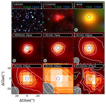
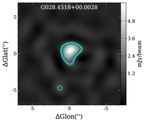
Figure 11: Radio source classified as HII region. Left: Panels are from top-left to bottom right: RGB image of UKIDSS three observed bands, RGB image of GLIMPSE three observed bands, WISE 12 $\mu$m, Hi-GAL 70 $\mu$m, Hi-GAL 160 $\mu$m, Hi-GAL 250 $\mu$m, Hi-GAL 500 $\mu$m, and ATLASGAL 870 $\mu$m. Right: Radio source detected in the GLOSTAR B-configuration image.

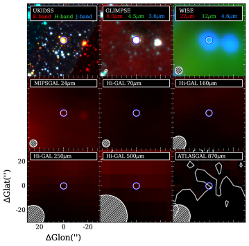
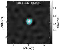
Figure 12: Same as Figure 11, but for radio source classified as radio star.

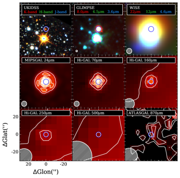
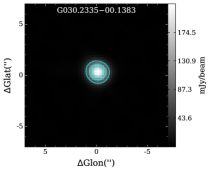
Figure 13: Same as Figure 11, but for radio source classified as PN.

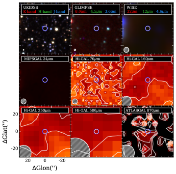
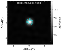
Figure 14: Same as Figure 11, but for radio source classified as EgC.

Appendix C MIR emission around identified HII region candidates

In this appendix, we present a series of images to show the MIR emission as seen by the GLIMPSE survey centered at the position of the identified HII region candidates. The images are boxes with size of $90^{\prime\prime}\times 90^{\prime\prime}$, and the false colors are defined to be red, green and blue for 8.0, 4.5 and 3.6$\,\mu$m.

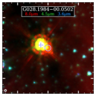
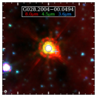
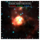
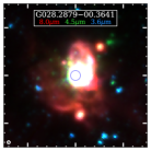
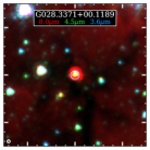
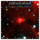
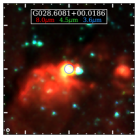
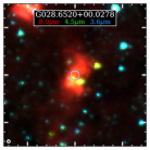
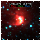
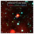
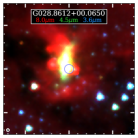
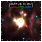
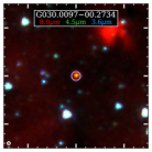
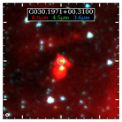
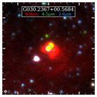
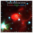
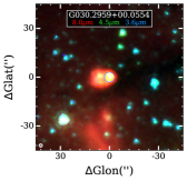
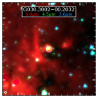
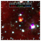
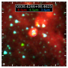
Figure 15: Three color GLIMPSE images at the position of the HII region candidates identified in the GLOSTAR B-configuration images. In the case of the fragmented HII regions, listed in Table 2, the position of additional fragment sources are shown with lime-white crosses.

Figure 1: Continuation.

Figure 1: Continuation.

References

- Anderson et al. (2014) Anderson, L. D., Bania, T. M., Balser, D. S., et al. 2014, ApJS, 212, 1
- Anderson et al. (2012) Anderson, L. D., Zavagno, A., Barlow, M. J., García-Lario, P., & Noriega-Crespo, A. 2012, A&A, 537, A1
- Bates et al. (2013) Bates, S. D., Lorimer, D. R., & Verbiest, J. P. W. 2013, MNRAS, 431, 1352
- Benjamin et al. (2003) Benjamin, R. A., Churchwell, E., Babler, B. L., et al. 2003, PASP, 115, 953
- Bertin & Arnouts (1996) Bertin, E. & Arnouts, S. 1996, A&AS, 117, 393
- Beuther et al. (2016) Beuther, H., Bihr, S., Rugel, M., et al. 2016, A&A, 595, A32
- Bihr et al. (2015) Bihr, S., Beuther, H., Ott, J., et al. 2015, A&A, 580, A112
- Bihr et al. (2016) Bihr, S., Johnston, K. G., Beuther, H., et al. 2016, A&A, 588, A97
- Bonaldi et al. (2019) Bonaldi, A., Bonato, M., Galluzzi, V., et al. 2019, MNRAS, 482, 2
- Brunthaler et al. (2021) Brunthaler, A., Menten, K. M., Dzib, S. A., et al. 2021, A&A, 651, A85
- Callingham et al. (2017) Callingham, J. R., Ekers, R. D., Gaensler, B. M., et al. 2017, ApJ, 836, 174
- Camilo et al. (2021) Camilo, F., Ransom, S. M., Halpern, J. P., & Roshi, D. A. 2021, arXiv e-prints, arXiv:2106.00386
- Carey et al. (2009) Carey, S. J., Noriega-Crespo, A., Mizuno, D. R., et al. 2009, PASP, 121, 76
- Carrasco-González et al. (2010) Carrasco-González, C., Rodríguez, L. F., Anglada, G., et al. 2010, Science, 330, 1209
- Casali et al. (2007) Casali, M., Adamson, A., Alves de Oliveira, C., et al. 2007, A&A, 467, 777
- Chakraborty et al. (2020) Chakraborty, A., Roy, N., Wang, Y., et al. 2020, MNRAS, 492, 2236
- Churchwell et al. (2009) Churchwell, E., Babler, B. L., Meade, M. R., et al. 2009, PASP, 121, 213
- Condon (1984) Condon, J. J. 1984, ApJ, 287, 461
- Contreras et al. (2013) Contreras, Y., Schuller, F., Urquhart, J. S., et al. 2013, A&A, 549, A45
- Cotton (2008) Cotton, W. D. 2008, PASP, 120, 439
- Csengeri et al. (2014) Csengeri, T., Urquhart, J. S., Schuller, F., et al. 2014, A&A, 565, A75
- Dallacasa (2003) Dallacasa, D. 2003, PASA, 20, 79
- Dallacasa et al. (2000) Dallacasa, D., Stanghellini, C., Centonza, M., & Fanti, R. 2000, A&A, 363, 887
- Deller et al. (2011) Deller, A. T., Brisken, W. F., Phillips, C. J., et al. 2011, PASP, 123, 275
- Dokara et al. (2021) Dokara, R., Brunthaler, A., Menten, K. M., et al. 2021, A&A, 651, A86
- Dzib et al. (2010) Dzib, S., Loinard, L., & Rodríguez, L. F. 2010, Rev. Mexicana Astron. Astrofis., 46, 153
- Dzib et al. (2021) Dzib, S. A., Forbrich, J., Reid, M. J., & Menten, K. M. 2021, ApJ, 906, 24
- Dzib et al. (2018) Dzib, S. A., Rodríguez, L. F., Karuppusamy, R., Loinard, L., & Medina, S.-N. X. 2018, ApJ, 866, 100
- Dzib et al. (2013) Dzib, S. A., Rodríguez, L. F., Loinard, L., et al. 2013, ApJ, 763, 139
- Fomalont et al. (1991) Fomalont, E. B., Windhorst, R. A., Kristian, J. A., & Kellerman, K. I. 1991, AJ, 102, 1258
- Forbrich et al. (2021) Forbrich, J., Dzib, S. A., Reid, M. J., & Menten, K. M. 2021, ApJ, 906, 23
- Forbrich et al. (2016) Forbrich, J., Rivilla, V. M., Menten, K. M., et al. 2016, ApJ, 822, 93
- Garay (1987) Garay, G. 1987, Rev. Mexicana Astron. Astrofis., 14, 489
- Garay et al. (1987) Garay, G., Moran, J. M., & Reid, M. J. 1987, ApJ, 314, 535
- Greisen (2003) Greisen, E. W. 2003, in Astrophysics and Space Science Library, Vol. 285, Information Handling in Astronomy - Historical Vistas, ed. A. Heck, 109
- Hales et al. (2012) Hales, C. A., Murphy, T., Curran, J. R., et al. 2012, MNRAS, 425, 979
- Halpern et al. (2012) Halpern, J. P., Gotthelf, E. V., & Camilo, F. 2012, ApJ, 753, L14
- Hambly et al. (2008) Hambly, N. C., Collins, R. S., Cross, N. J. G., et al. 2008, MNRAS, 384, 637
- Helfand et al. (2007) Helfand, D. J., Gotthelf, E. V., Halpern, J. P., et al. 2007, ApJ, 665, 1297
- Hewett et al. (2006) Hewett, P. C., Warren, S. J., Leggett, S. K., & Hodgkin, S. T. 2006, MNRAS, 367, 454
- Hoare et al. (2012) Hoare, M. G., Purcell, C. R., Churchwell, E. B., et al. 2012, PASP, 124, 939
- Hodgkin et al. (2009) Hodgkin, S. T., Irwin, M. J., Hewett, P. C., & Warren, S. J. 2009, MNRAS, 394, 675
- Huynh et al. (2015) Huynh, M. T., Bell, M. E., Hopkins, A. M., Norris, R. P., & Seymour, N. 2015, MNRAS, 454, 952
- Huynh et al. (2020) Huynh, M. T., Seymour, N., Norris, R. P., & Galvin, T. 2020, MNRAS, 491, 3395
- Intema et al. (2017) Intema, H. T., Jagannathan, P., Mooley, K. P., & Frail, D. A. 2017, A&A, 598, A78
- Kalcheva et al. (2018) Kalcheva, I. E., Hoare, M. G., Urquhart, J. S., et al. 2018, A&A, 615, A103
- Kounkel et al. (2017) Kounkel, M., Hartmann, L., Loinard, L., et al. 2017, ApJ, 834, 142
- Lawrence et al. (2007) Lawrence, A., Warren, S. J., Almaini, O., et al. 2007, MNRAS, 379, 1599
- Lucas et al. (2008) Lucas, P. W., Hoare, M. G., Longmore, A., et al. 2008, MNRAS, 391, 136
- Maan et al. (2018) Maan, Y., Bassa, C., van Leeuwen, J., Krishnakumar, M. A., & Joshi, B. C. 2018, ApJ, 864, 16
- Marleau et al. (2008) Marleau, F. R., Noriega-Crespo, A., Paladini, R., et al. 2008, AJ, 136, 662
- Medina et al. (2018) Medina, S. N. X., Dzib, S. A., Tapia, M., Rodríguez, L. F., & Loinard, L. 2018, A&A, 610, A27
- Medina et al. (2019) Medina, S. N. X., Urquhart, J. S., Dzib, S. A., et al. 2019, A&A, 627, A175
- Menten et al. (2007) Menten, K. M., Reid, M. J., Forbrich, J., & Brunthaler, A. 2007, A&A, 474, 515
- Molinari et al. (2016) Molinari, S., Schisano, E., Elia, D., et al. 2016, A&A, 591, A149
- Molinari et al. (2010) Molinari, S., Swinyard, B., Bally, J., et al. 2010, PASP, 122, 314
- Nguyen et al. (2021) Nguyen, H., Rugel, M. R., Menten, K. M., et al. 2021, A&A, 651, A88
- Nguyen et al. (2022) Nguyen, H., Rugel, M. R., Murugeshan, C., et al. 2022, arXiv e-prints, arXiv:2207.10548
- Ortiz-León et al. (2021) Ortiz-León, G. N., Menten, K. M., Brunthaler, A., et al. 2021, A&A, 651, A87
- Phillips & Marquez-Lugo (2011) Phillips, J. P. & Marquez-Lugo, R. A. 2011, MNRAS, 410, 2257
- Prandoni et al. (2018) Prandoni, I., Guglielmino, G., Morganti, R., et al. 2018, MNRAS, 481, 4548
- Purcell et al. (2013) Purcell, C. R., Hoare, M. G., Cotton, W. D., et al. 2013, ApJS, 205, 1
- Purser et al. (2016) Purser, S. J. D., Lumsden, S. L., Hoare, M. G., et al. 2016, MNRAS, 460, 1039
- Reid et al. (2014) Reid, M. J., Menten, K. M., Brunthaler, A., et al. 2014, ApJ, 783, 130
- Rodríguez et al. (2012) Rodríguez, L. F., González, R. F., Montes, G., et al. 2012, ApJ, 755, 152
- Schuller et al. (2009) Schuller, F., Menten, K. M., Contreras, Y., et al. 2009, A&A, 504, 415
- Smolčić et al. (2017) Smolčić, V., Delvecchio, I., Zamorani, G., et al. 2017, A&A, 602, A2
- Urquhart et al. (2014) Urquhart, J. S., Csengeri, T., Wyrowski, F., et al. 2014, A&A, 568, A41
- Urquhart et al. (2013) Urquhart, J. S., Thompson, M. A., Moore, T. J. T., et al. 2013, MNRAS, 435, 400
- Vargas-González et al. (2021) Vargas-González, J., Forbrich, J., Dzib, S. A., & Bally, J. 2021, MNRAS, 506, 3169
- Wang et al. (2020) Wang, Y., Beuther, H., Rugel, M. R., et al. 2020, A&A, 634, A83
- Wang et al. (2018) Wang, Y., Bihr, S., Rugel, M., et al. 2018, A&A, 619, A124
- Wenger et al. (2000) Wenger, M., Ochsenbein, F., Egret, D., et al. 2000, A&AS, 143, 9
- Williams et al. (2016) Williams, W. L., van Weeren, R. J., Röttgering, H. J. A., et al. 2016, MNRAS, 460, 2385
- Wilman et al. (2008) Wilman, R. J., Miller, L., Jarvis, M. J., et al. 2008, MNRAS, 388, 1335
- Wilner et al. (1999) Wilner, D. J., Reid, M. J., & Menten, K. M. 1999, ApJ, 513, 775
- Windhorst et al. (1985) Windhorst, R. A., Miley, G. K., Owen, F. N., Kron, R. G., & Koo, D. C. 1985, ApJ, 289, 494
- Wright et al. (2010) Wright, E. L., Eisenhardt, P. R. M., Mainzer, A. K., et al. 2010, AJ, 140, 1868
- Wu et al. (2014) Wu, Y. W., Sato, M., Reid, M. J., et al. 2014, A&A, 566, A17
- Yang et al. (2019) Yang, A. Y., Thompson, M. A., Tian, W. W., et al. 2019, MNRAS, 482, 2681
- Yang et al. (2021) Yang, A. Y., Urquhart, J. S., Thompson, M. A., et al. 2021, A&A, 645, A110