Adaptive Smoothness-weighted Adversarial Training for Multiple Perturbations with Its Stability Analysis

Abstract

Adversarial Training (AT) has been demonstrated as one of the most effective methods against adversarial examples. While most existing works focus on AT with a single type of perturbation (e.g., the $\ell_{\infty}$ attacks), DNNs are facing threats from different types of adversarial examples. Therefore, adversarial training for multiple perturbations (ATMP) is proposed to generalize the adversarial robustness over different perturbation types (in $\ell_{1}$, $\ell_{2}$, and $\ell_{\infty}$ norm-bounded perturbations). However, the resulting model exhibits trade-off between different attacks. Meanwhile, there is no theoretical analysis of ATMP, limiting its further development. In this paper, we first provide the smoothness analysis of ATMP and show that $\ell_{1}$, $\ell_{2}$, and $\ell_{\infty}$ adversaries give different contributions to the smoothness of the loss function of ATMP. Based on this, we develop the stability-based excess risk bounds and propose adaptive smoothness-weighted adversarial training for multiple perturbations. Theoretically, our algorithm yields better bounds. Empirically, our experiments on CIFAR10 and CIFAR100 achieve the state-of-the-art performance against the mixture of multiple perturbations attacks.

1 Introduction

Deep neural networks (DNNs) are shown to be vulnerable to adversarial examples (Goodfellow et al.,, 2014; Szegedy et al.,, 2013), where a small and malicious perturbation can cause incorrect predictions. Adversarial training (AT) (Madry et al.,, 2017), which augments training data with $\ell_{p}$ norm-bounded adversarial examples, is one of the most effective methods to increase the robustness of DNNs against adversarial attacks. Currently, most existing works focus on adversarial training with a single type of attack, e.g., the $\ell_{\infty}$ attack (Raghunathan et al.,, 2019; Gowal et al.,, 2020). However, some recent works (Tramèr and Boneh,, 2019) have experimentally demonstrated that the DNNs trained with a single type of adversarial attack cannot provide well defense against other types of adversarial examples. Fig. 1 (a) provides an example on CIFAR-10. The plot shows that the $\ell_{1}$ adversarial training cannot defend the $\ell_{2}$ and $\ell_{\infty}$ attacks (its robust accuracy are 0%). The $\ell_{\infty}$ adversarial training can provide some extent of defense against $\ell_{1}$ and $\ell_{2}$ attacks (with accuracy being 17.19% and 53.91%). But it is not comparable to the performance of $\ell_{1}$ and $\ell_{2}$ adversarial training, 89.84%, and 61.72%, respectively.

For better robustness against different types of attacks, Tramer et al., (Tramèr and Boneh,, 2019) extends adversarial training against multiple perturbations (ATMP) (typically the $\ell_{1}$, $\ell_{2}$, and $\ell_{\infty}$ attacks). Specifically, they consider two types of objective functions. The first one is the average of all perturbations (AVG), where the inner maximization problem of adversarial training finds adversarial examples for all types of attacks. The second one is worst-case perturbation (WST), where the inner maximization problem finds the adversarial examples with the largest loss within the union of the $\ell_{p}$ norm balls. Following these settings, researchers have proposed different algorithms to solve these two problems. Representative works are multi-steepest descent (MSD) (Maini et al.,, 2020), and stochastic adversarial training (SAT) (Madaan et al.,, 2020), which use different strategies to find adversarial examples in the $\ell_{p}$-norm balls and obtain some improvements comparing to the MAX and AVG.

However, there exist several crucial issues that are unsolved w.r.t. ATMP. Firstly, the optimization process of ATMP is highly unstable compared to that of AT or standard training. Fig. 1 (c) and (d) give an example. The test robust accuracy fluctuates between different training epochs. Secondly, it is quite difficult to achieve a satisfying trade-off between different attacks. None of them achieves the best performance against all of the three attacks, as shown in Fig. 1 (b). Different algorithms tend to find sub-optimal around different local minima, resulting in a model perform well in one perturbation while worse defend against others. Last but most important, there is no theoretical study of ATMP currently. The exploration of ATMP methods is usually experimentally designed, without any theoretical guidelines.

Figure 1: Crucial issues of adversarial training for multiple perturbations. (a) Performance of adversarial training with a single type perturbation against other type attacks. (b) Trade-off between different types of adversaries of four algorithms for ATMP. (c) Robust test accuracy fluctuate between different epochs using MAX. (d) Robust test accuracy fluctuate between different epochs using MSD.

In this work, we first study the smoothness and the loss landscape of ATMP. We show that the smoothness of $\ell_{1}$, $\ell_{2}$, and $\ell_{\infty}$ adversaries give different contributions to the smoothness of ATMP. It motivates us to study a question:

How to use the smoothness properties of different $\ell_{p}$ adversaries to design algorithms for ATMP?

We study this question using the notion of uniform stability. In uniform stability analysis, excess risk, which is the sum of optimization error and generalization error, is highly related to the smoothness of the loss function. The formal and stability analysis and excess risk upper bound of ATMP are provided in Thm. 5.1. Inspired by the analysis, we propose adaptive smoothness-weighted adversarial training for multiple perturbations to improve the excess risk bound. Theoretically, our algorithms yields better bound (See our main results in Thm. 5.2 and Thm. 5.3). Experimental results on CIFAR-10 and CIFAR-100 show that this technique mitigates the above issues and improves the performance of ATMP. Our solution achieves the state-of-the-art performance against the mixture of multiple perturbations attacks.

Our contributions are listed as follow:

1. We provide a comprehensive smoothness analysis of adversarial training for single and multiple perturbations.

2. We provide a uniform stability analysis on ATMP. Based on the analysis, we propose our stability-inspired algorithm: adaptive smoothness-weighted adversarial training for multiple perturbations.

3. Theoretically, our algorithms yields better excess risk bound. Experimentally, we obtain an improvement on robust accuracy, achieving the state-of-the-art performance on CIFAR-10 and CIFAR-100.

2 Related Work

In this section, we first introduce the standard adversarial training with a single type of perturbation, as well as its theoretical analysis. We then introduce the adversarial training against multiple perturbations.

Adversarial training

Adversarial training (AT) has been demonstrated to be one of the most effective ways to increase the adversarial robustness (Szegedy et al.,, 2013). The key idea of AT is to augment the training set with adversarial examples during training. Currently, most AT-based methods are trained with a single type of adversarial examples, and the $\ell_{p}$ (p=1, 2, or $\infty$) is commonly used to generate adversarial examples during training (Madry et al.,, 2017). It is shown that AT overfits the adversarial examples on the training set and generalizes badly on the test sets. Many approaches have been proposed to increase the adversarial generalization (Raghunathan et al.,, 2019; Schmidt et al.,, 2018). Meanwhile, there have been some attempts for the theoretical understanding of adversarial training, mainly focusing on the convergence properties and generalization bound. For example, the work of (Gao et al.,, 2019) studies the convergence of adversarial training in the neural tangent kernel (NTK) regime. Liu et al. study the smoothness of the loss function of adversarial training (Liu et al., 2020b, ). In terms of generalization bound, the work of (Yin et al.,, 2019; Awasthi et al.,, 2020) study the generalization bound in terms of Rademacher complexity. The work of (Gao et al.,, 2019) considers the VC-dimension bound of adversarial training. Xing et al. (Xing et al.,, 2021) study the generalization of adversarial linear regression.

Adversarial robustness against multiple perturbations models

Recently, some works have demonstrated that adversarial training with a single type of perturbation cannot provide well defense against other types of adversarial attacks (Tramèr and Boneh,, 2019) and several ATMP algorithms have been proposed accordingly (Maini et al.,, 2020; Madaan et al.,, 2020; Zhang et al.,, 2021; Stutz et al.,, 2020). The work of (Tramèr and Boneh,, 2019) proposed to augment different types of adversarial examples into adversarial training and developed two augmentation strategies, i.e., MAX and AVG. The MAX adopts the worst-case adversarial example among different attacks, while the AVG takes all types of adversarial examples into training. Following the above pipeline, some later works developed different aggregation strategies (e.g., the MSD (Maini et al.,, 2020), and SAT (Madaan et al.,, 2020)) for better robustness or training efficiency. While these works can boost the adversarial robustness against multiple perturbations to some extent, the training process of ATMP is highly unstable, and there is no theoretical analysis about this. The theoretical understanding of the training difficulty of ATMP is important for the further development of adversarial robustness for multiple perturbations. Besides, there have also been some other works for adversarial robustness against multiple perturbations, such as Ensemble models (Maini et al.,, 2021; Cheng et al.,, 2021), Prepossessing (Nandy et al.,, 2020) and Neural architectures search (NAS) (Liu et al., 2020a, ). The weakness of ensemble models or prepossess methods is that the performance is highly related to the classification quality or detection of different types of adversarial examples. These methods either have lower performance or consider different tasks from the work we considered. Therefore, we mainly compare the algorithms MAX, AVG, MSD, and SAT in this work.

3 Preliminaries of Adversarial Training for Multiple Perturbations

Adversarial training is an approach to train a classifier that minimizes the worst-case loss within a norm-bounded constraint. Let $g(\theta,z)$ be the loss function of the standard counterpart. Given training dataset ${\mathcal{S}}=\{z_{i}\}_{i=1\cdots n}$, the optimization problem of adversarial training is

$$\min_{\theta}\frac{1}{n}\sum_{i=1}^{n}\max_{\|z_{i}-z_{i}^{\prime}\|_{p}\leq\epsilon_{p}}g(\theta,z_{i}^{\prime}),$$ (3.1)

where $\epsilon_{p}$ is the perturbation threshold, $p=1,2$ or $\infty$ for different types of attacks. Usually, $g$ can also be written in the form of $\ell(f_{\theta}({\bm{x}}),y)$, where $f_{\theta}$ is the neural network to be trained and $({\bm{x}},y)$ is the input-label pair. Adversarial training aims to train a model against a single type of $\ell_{p}$ attack. As AT with a single type of attacks may not be effecting under other types of attacks, adversarial training for multiple perturbations are proposed (Tramèr and Boneh,, 2019). Following the aforementioned literature, we consider the case that $p=1,2,\infty$. Two formulations can be use to tackle this problem.

Worst-case perturbation (WST)

The optimization problem of WST is formulated as follow,

$$\min_{\theta}\frac{1}{n}\sum_{i=1}^{n}\max_{p\in\{1,2,\infty\}}\max_{\|z_{i}-z_{i}^{\prime}\|_{p}\leq\epsilon_{p}}g(\theta,z_{i}^{\prime}).$$ (3.2)

WST aims to find the worst adversarial examples within the union of the three norm constraints for the inner maximization problem. The outer minimization problem updates model parameters $\theta$ to fit these adversarial examples. The MAX strategy (Tramèr and Boneh,, 2019) are proposed for the optimization problem in Eq. (3.2). In each inner iteration, MAX takes the maximum loss on these three adversarial examples. Another algorithm for the optimization problem in Eq. (3.2) is multi-steepest descent (MSD) (Maini et al.,, 2020). In each PGD step in the inner iteration, MSD selects the worst among $\ell_{1}$, $\ell_{2}$, and $\ell_{\infty}$ attacks.

Average of all perturbations (AVG)

The optimization problem of AVG is formulated as follow

$$\min_{\theta}\frac{1}{n}\sum_{i=1}^{n}\mathbb{E}_{p\sim\{1,2,\infty\}}\max_{\|z_{i}-z_{i}^{\prime}\|_{p}\leq\epsilon_{p}}g(\theta,z_{i}^{\prime}),$$ (3.3)

where $p\sim\{1,2,\infty\}$ uniformly at random. The goal of the minimax problem in Eq. (3.3) is to train the neural networks using data augmented with all three types of adversarial examples. The AVG strategy (Tramèr and Boneh,, 2019) and the stochastic adversarial training (SAT) (Madaan et al.,, 2020) are two algorithms to solve the problem in Eq. (3.3). In each inner iteration, AVG takes the average loss on these three adversarial examples and SAT randomly chooses one type of adversarial example among $\ell_{1}$, $\ell_{2}$, and $\ell_{\infty}$ attacks.

Problem WST and AVG are similar but slightly different problems. WST aims to defend union attacks, i.e., the optimal attack within the union of multiple perturbations. AVG aims to defend mixture attacks, i.e., the attacker randomly pick one $\ell_{p}$ attack. In this paper, we mainly focus on problem AVG, we also discuss some solutions for problem WST.

4 Smoothness Analysis

We first study the smoothness of the minimax problems in Eq. (3.2) and (3.3). To simplify the notation, let

$$h^{p}(\theta,z) = \max_{\|z-z^{\prime}\|_{p}\leq\epsilon_{p}}g(\theta,z^{\prime}),$$

$$h^{avg}(\theta,z) = \mathbb{E}_{p\sim\{1,2,\infty\}}\max_{\|z-z^{\prime}\|_{p}\leq\epsilon_{p}}g(\theta,z^{\prime}),$$

$$h^{wst}(\theta,z) = \max_{p\in\{1,2,\infty\}}\max_{\|z-z^{\prime}\|_{p}\leq\epsilon_{p}}g(\theta,z^{\prime})$$

be the loss function of standard adversarial training, worst-case multiple perturbation adversarial training, and average of all perturbations adversarial training, respectively. The population and empirical risks are the expectation and average of $h^{st}(\cdot)$, respectively. We use $R_{\mathcal{D}}^{st}(\theta)$ and $R_{S}^{st}(\theta)$ to denote the population and empirical risk for adversarial training with different strategy, i.e. $\text{st}\in\{1,2,\infty,\text{wst},\text{avg}\}$.

Case study: Linear regression

We use a simple case, adversarial linear regression, to illustrate the smoothness of the optimization problem of (3.2) and (3.3). Let $f_{\theta}({\bm{x}})=\theta^{T}{\bm{x}}$ and $\ell(\theta^{T}x,y)=|\theta^{T}{\bm{x}}-y|^{2}$, we have the following proposition.

Proposition 4.1.

Let ${\bm{X}}=[{\bm{x}}_{1},\cdots,{\bm{x}}_{n}]^{T}$, $y=[y_{1},\cdots,y_{n}]^{T}$, and $\delta=[\delta_{1},\cdots,\\ \delta_{n}]^{T}$, we have

$$R_{S}^{p}(\theta) = [\|{\bm{X}}\theta-y\|_{2}+\sqrt{n}\epsilon_{p}\|\theta\|_{p^{*}}]^{2},$$

$$R_{S}^{wst}(\theta) = \max_{p\in\{1,2,\infty\}}[\|{\bm{X}}\theta-y\|_{2}+\sqrt{n}\epsilon_{p}\|\theta\|_{p^{*}}]^{2},$$

$$R_{S}^{avg}(\theta) = \mathbb{E}_{p\in\{1,2,\infty\}}[\|{\bm{X}}\theta-y\|_{2}+\sqrt{n}\epsilon_{p}\|\theta\|_{p^{*}}]^{2}.$$

The proof is deferred to A. From Proposition 4.1, the loss landscape of adversarial training is non-smooth because of the term $\|\theta\|_{p^{*}}$. Specifically, the loss function of $\ell_{2}$ adversarial training is non-smooth at $\theta=0$. For $\ell_{1}$ adversarial training, the loss function is non-smooth at $|\theta_{i}|=|\theta_{j}|,\forall i,j$. For $\ell_{\infty}$ adversarial training, the loss function is non-smooth at $\theta_{i}=0,\forall i$. For adversarial training for multiple perturbations, the loss function is non-smooth at both $\theta_{i}=0,\forall i$ and $|\theta_{i}|=|\theta_{j}|,\forall i,j$. The non-smooth region of the loss function of ATMP is the union of that of the single perturbation cases. Different $\ell_{p}$ adversaries give different contribution to the smoothness of the loss function of ATMP.

In Fig. 2, we give a numerical simulation and demonstrate the loss landscape in a two-dimensional case. In $\ell_{2}$ adversarial training, the loss landscape is smooth almost everywhere, except the original point. In $\ell_{1}$ and $\ell_{\infty}$ cases, the non-smooth region is a ‘cross’. In the cases of WST and AVG, the non-smooth region is the union of two ‘crosses’.

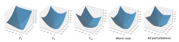
Figure 2: Loss landscape of adversarial linear regression for single and multiple perturbations.

General nonlinear model

Now let us consider general nonlinear models. Following the work of (Sinha et al.,, 2017), without loss of generality, let us assume

Assumption 4.1.

The function $g$ satisfies the following Lipschitzian smoothness conditions:

$$\|g(\theta_{1},z)-g(\theta_{2},z)\|\leq L\|\theta_{1}-\theta_{2}\|,$$

$$\|\nabla_{\theta}g(\theta_{1},z)-\nabla_{\theta}g(\theta_{2},z)\|\leq L_{\theta}\|\theta_{1}-\theta_{2}\|,$$

$$\|\nabla_{\theta}g(\theta,z_{1})-\nabla_{\theta}g(\theta,z_{2})\|\leq L_{\theta z}\|z_{1}-z_{2}\|,$$

$$\|\nabla_{z}g(\theta_{1},z)-\nabla_{\theta}g(\theta_{2},z)\|\leq L_{z\theta}\|\theta_{1}-\theta_{2}\|.$$

Assumption 4.1 assumes that the loss function is smooth (in zeroth-order and first-order). While ReLU activation function is non-smooth, recent works (Allen-Zhu et al.,, 2019; Du et al.,, 2019) showed that the loss function of overparamterized DNNs is semi-smooth. It helps justify Assumption 4.1. Under Assumption 4.1, the following Lemma Provide the smoothness of ATMP.

Lemma 4.1.

Under Assumption 4.1, assuming in addtion that $g(\theta,z)$ is locally $\mu_{p}$-strongly concave for all $z\in\mathcal{Z}$ in $\ell_{p}$-norm. $\forall\theta_{1},\theta_{2}$ and $\forall z\in\mathcal{Z}$, the following properties hold.

1. (Lipschitz function.) $\|h^{st}(\theta_{1},z)-h^{st}(\theta_{2},z)\|\leq L\|\theta_{1}-\theta_{2}\|$.

2. (Gradient Lipschitz.) If we Then, $\|\nabla_{\theta}h^{st}(\theta_{1},z)-\nabla_{\theta}h^{st}(\theta_{2},z)\|\leq\beta_{st}\|\theta_{1}-\theta_{2}\|$, where

   $$\beta_{st}=\begin{cases}L_{\theta z}L_{z\theta}/\mu_{st}+L_{\theta}&\text{st}\in\{1,2,\infty\},\\ L_{\theta z}L_{z\theta}/\min_{p}\mu_{p}+L_{\theta}&\text{st}=\text{wst},\\ \mathbb{E}_{p\sim\{1,2,\infty\}}\beta_{p}&\text{st}=\text{avg}.\end{cases}$$

Proof: see A.2. Lemma 4.1 shows that adversarial surrogate loss in different $\ell_{p}$ adversaries have different smoothness in strongly-concave case. This property is not specific for strongly-concave case. The analysis of non-strongly-concavity case is provided in A.3. Lemma 4.1 motivates us to study a question:

How to achieve better performance on adversarial robustness against different $\ell_{p}$ adversarial attacks utilizing the smoothness properties?

In the next section, we first discuss the stability analysis of ATMP. Then, we discuss how to utilize the smoothness-properties of different $\ell_{p}$ adversaries to obtain smaller generalization bound.

5 Stability-based Excess Risk Analysis

In this section, we focus on the problem AVG. Assuming that the target model are facing $P$ potential attacks. In the above setting, $P=3$ and the three attacks are $\ell_{1}$, $\ell_{2}$, and $\ell_{\infty}$ attacks. The test and training performance against mixture attacks is

$$R_{\cal D}(\theta)=\frac{1}{P}\sum_{p=1}^{P}R_{\cal D}^{p}(\theta)\ \ \text{and}\ \ R_{S}(\theta)=\frac{1}{P}\sum_{p=1}^{P}R_{S}^{p}(\theta),$$

respectively.

Risk Decomposition

Let $\theta^{*}$ and $\bar{\theta}$ be the optimal solution of $R_{\cal D}(\theta)$ and $R_{S}(\theta)$, respectively. Then for the algorithm output $\hat{\theta}=A(S)$, the excess risk can be decomposed as

$$R_{\cal D}(\hat{\theta})-R_{\cal D}(\theta^{*})$$ (5.1)

$$= \underbrace{R_{\cal D}(\hat{\theta})-R_{S}(\hat{\theta})}_{\mathcal{E}_{gen}}+\underbrace{R_{S}(\hat{\theta})-R_{S}(\bar{\theta})}_{\mathcal{E}_{opt}}+ \underbrace{R_{S}(\bar{\theta})-R_{S}(\theta^{*})}_{\leq 0}+\underbrace{R_{S}(\theta^{*})-R_{\cal D}(\theta^{*})}_{\mathbb{E}=0}.$$

To control the excess risk, we need to control the generalization gap $\mathcal{E}_{gen}$ and the optimization gap $\mathcal{E}_{opt}$. In the rest of the paper, we use $\mathcal{E}_{gen}$ and $\mathcal{E}_{opt}$ to denote the expectation of the generalization and optimization gap. The smoothness of the loss function is highly related to the generalization gap $\mathcal{E}_{gen}$ and the optimization gap $\mathcal{E}_{opt}$, we first provide the the optimization error bound (Nemirovski et al.,, 2009) and stability-based generalization bound (Hardt et al.,, 2016) for running SGD on Eq. (3.3).

Theorem 5.1.

Under Assumption 4.1, assuming in addition that $g(\theta,z)$ is convex in $\theta$ for all given $z\in\mathcal{Z}$. Let $D=\|\theta^{0}-\theta^{*}\|$, where $\theta^{0}$ is the initialization of SGD. Suppose that we run SGD with step sizes $\alpha\leq 1/\beta_{avg}$ for $T$ steps. Then, adversarial training satisfies

$$\mathcal{E}_{opt}\leq\frac{D^{2}+L^{2}T\alpha^{2}}{2T\alpha},\ \ \mathcal{E}_{gen}\leq\frac{2L^{2}T\alpha}{n}.$$ (5.2)

Therefore, the $\beta$-gradient Lipschitz constant of the loss function is related to the choice of stepsize, the optimization and generalization bound. In the loss function of AVG, each of the $\ell_{p}$ adversarial loss have different Lipschitz constant $\beta_{p}$. It motivates us to study whether we can assign different stepsize to different $\ell_{p}$ adversarial loss to improve the excess risk.

5.1 Smoothness-weighted Adversarial Training for Multiple Perturbations

Considering the algorithm

$$\theta^{t+1}=\theta^{t}-\frac{1}{P}\bigg{[}\alpha_{1}^{t}\nabla R_{S}^{1}(\theta^{t})+\cdots+\alpha_{P}^{t}\nabla R_{S}^{P}(\theta^{t})\bigg{]},$$ (5.3)

In each of the iterations $t$, we assign stepsize $\alpha_{p}^{t}$ to the $p^{th}$-tasks.

Properties of Update Rules

We define $G_{z}(\theta)=\theta-\frac{1}{P}\sum_{p=1}^{P}\alpha_{p}\nabla h^{p}(\theta,z)$ be the update rule. The following lemma holds.

Lemma 5.1 (Non-expansive).

Assuming that the function $h^{p}(\theta,z)$ is $\beta_{p}$-gradient Lipschitz, convex for all $z\in\mathcal{Z}$. Then, $\forall\theta_{1},\theta_{2}$ and $\forall z\in\mathcal{Z}$, for $\alpha_{p}\leq 1/\beta_{p}$, we have $\|G_{z}(\theta_{1})-G_{z}(\theta_{2})\|\leq\|\theta_{1}-\theta_{2}\|.$

Proof of Lemma 5.1 is deferred to A.4. Based on Lemma 5.1, we have the following generalization guarantee for problem AVG.

Theorem 5.2 (Generalization bounds of smoothness-weighted learning rate).

Under Assumption 4.1, assume in addition that $h^{p}(\theta,z)$ is convex in $\theta$ for all given $z\in\mathcal{Z}$. Suppose that we run Algorithm 1 with step sizes $\alpha_{p}\leq 1/\beta_{p}$ for $T$ steps. Then, adversarial training satisfies uniform stability with

$$\mathcal{E}_{gen}\leq\frac{2L^{2}T\sum_{p=1}^{P}\alpha_{p}/P}{n}.$$

Proof: The proof is based on Lemma 5.1 and defer to A.5.

Let $\alpha_{sw}^{t}=(\alpha_{1}^{t}+\cdots+\alpha_{P}^{t})/P$, we have $\mathcal{E}_{gen}\leq 2L^{2}T\alpha_{sw}/n$.

Theorem 5.3 (Optimization bounds of smoothness-weighted learning rate).

Under Assumption 4.1, assume in addition that $h^{p}(\theta,z)$ is convex in $\theta$ for all given $z\in\mathcal{Z}$. Suppose that we run SGD with step sizes $\alpha_{p}^{t}\leq 1/\beta_{p}$ for $T$ steps. Then, adversarial training satisfies

$$\mathcal{E}_{opt}\leq\frac{D^{2}+L^{2}T\alpha_{sw}^{2}}{2T\alpha_{sw}}+B\frac{\sum_{p=1}^{P}|\alpha_{sw}-\alpha_{p}|}{\alpha_{sw}}.$$

The proof is deferred to A.6. The first term has the same form as Theorem 5.1, the second term is an additional bias term introduced by the smoothness-weighted learning rate. Combining the $\mathcal{E}_{opt}$ and $\mathcal{E}_{gen}$, we have

$$\mathcal{E}_{gen}+\mathcal{E}_{opt}\leq\underbrace{\frac{2L^{2}T\alpha_{sw}}{n}+\frac{D^{2}+L^{2}T\alpha_{sw}^{2}}{2T\alpha_{sw}}}_{\text{The same as Thm. \ref{thm:stdbound} with different $\alpha$}}+\underbrace{B\frac{\sum_{p=1}^{P}|\alpha_{sw}-\alpha_{p}|}{\alpha_{sw}}}_{\text{bias term}}.$$

Optimizing the first two terms with respective to $\alpha$, we have

$$\alpha^{*}=\frac{D\sqrt{n}}{L\sqrt{T(n+2T)}}.$$

In adversarial training, $T$ cannot be too large because of robust overfitting. Then, The right-hand-side may be too large and we may not choose $\alpha^{*}$ as the learning rate. We need a larger $\alpha$ to reduce the first two term. From the previous dicussion, we have

$$\alpha_{avg}\leq\frac{P}{\beta_{1}+\cdots+\beta_{P}}\ and\ \alpha_{sw}\leq\frac{\frac{1}{\beta_{1}}+\cdots+\frac{1}{\beta_{P}}}{P}.$$

Therefore, $\alpha_{sw}$ can be view as the inverse of the harmonic mean of $\beta_{p}$ and $\alpha_{avg}$ can be view as the inverse of the arithmetic mean of $\beta_{p}$. $\alpha_{sw}$ is larger and reduce the first two terms when $T$ is small.

Overall, we need smaller $T$ and carefully chosen learning rates to speed up adversarial training to avoid robust overfitting. Smoothness-weighted learning rate gives us a way to increase the learning rate. As a side-effect, it introduce an additional bias term. In experiments, we will show that $\alpha_{sw}$ can improve the test performance.

5.2 Proposed Method

In practice, $\beta_{p}$ is unknown. We adaptively estimate $\beta_{p}$ in each iterations. By descent Lemma, we have

$$h^{p}(\theta_{t})-h^{p}(\theta^{*})\leq\nabla h^{p}(\theta^{*})\langle\theta_{t}-\theta^{*}\rangle+\frac{\beta_{p}}{2}\|\theta_{t}-\theta^{*}\|^{2}=\frac{\beta_{p}}{2}\|\theta_{t}-\theta^{*}\|^{2}.$$

It suggests us to use the following rules

$$\alpha_{p}^{t}\propto\frac{1}{\beta_{p}}\propto\frac{\|\theta_{t}-\theta^{*}\|^{2}}{h^{p}(\theta_{t})-h^{p}(\theta^{*})}\propto\frac{1}{h^{p}(\theta_{t})-h^{p}(\theta^{*})}$$

to approximate $\beta_{p}$ and to choice $\alpha_{p}^{t}$. Assuming that $h^{p}(\theta^{*})=0$, we can use $\sum_{p}h^{p}(\theta_{t})/(Ph^{p}(\theta_{t}))$ as the weight of $\alpha_{p}^{t}$. Given the initial learning rate schedule $\alpha^{1},\cdot,\alpha^{T}$, the following Algorithm 1 is the proposed adaptive smoothness-weighted ATMP.

Algorithm 1 Adaptive Smoothness-Weighted ATMP

  Inputs: classifier $f_{\theta}({\bm{x}},y)$, dataset $\{{\bm{x}}_{i},y_{i}\}_{i=1,\cdots,n}$.

  Initialize learning rate schedule $\alpha^{1},\cdot,\alpha^{T}$.

  for $t=1$ to $T$ do

     for $p=1$ to $P$ do

        

$$\mathcal{L}_{p}=\frac{1}{n}\sum_{i=1}^{n}\max_{\|\delta_{i}\|_{p}\leq\epsilon_{p}}\ell(f_{\theta_{t}}({\bm{x}}_{i}+\delta_{i},y_{i}).$$

     end for

     Define $\mathcal{L}=\mathcal{L}_{1}+\cdots+\mathcal{L}_{P}$.

     Update $\alpha_{p}^{t}=\alpha^{t}\times\mathcal{L}/P\mathcal{L}_{P}$, $p=1,2,\cdots,P$.

     Update

$$\theta^{t+1}=\theta^{t}-\frac{1}{P}\bigg{[}\alpha_{1}^{t}\nabla R_{S}^{1}(\theta^{t})+\cdots+\alpha_{P}^{t}\nabla R_{S}^{P}(\theta^{t})\bigg{]},$$

  end for

6 Experiments

Table 1: Test accuracy (%) of different algorithms (MAX, AVG, MSD, SAT, and ADT) against $\ell_{1}$, $\ell_{2}$, and $\ell_{\infty}$ attacks on CIFAR-10.

Dataset		CIFAR-10
Attack methods		clean	$\ell_{1}$	$\ell_{2}$	$\ell_{\infty}$	Union	Mix
AT	$\ell_{1}$	93.22	89.81	0.00	0.00	0.00	29.98
	$\ell_{2}$	88.66	41.41	61.72	39.84	18.41	47.66
	$\ell_{\infty}$	84.94	17.19	53.91	46.88	40.11	39.32
WST (Eq. 3.2)	MAX	84.96	52.63	64.74	46.93	46.08$\pm$0.43	54.77$\pm$0.22
	MSD	83.51	54.92	67.68	49.88	46.99$\pm$0.23	57.49$\pm$0.11
AVG (Eq. 3.3)	AVG	85.28	58.78	68.08	43.87	43.28$\pm$0.55	56.91$\pm$0.34
	SAT	85.23	58.68	67.77	43.59	43.12$\pm$1.89	56.68$\pm$1.01
	ADT	85.87	61.81	69.61	46.64	46.05$\pm$0.31	59.16$\pm$0.09

6.1 Performance of ADT

Datasets and Classification Models

We conduct experiments on two widely used benchmark datasets: CIFAR-10 and CIFAR-100 (Krizhevsky et al.,, 2009). CIFAR-10 includes 50k training images and 10k test images with 10 classes. CIFAR-100 includes 50k training images and 10k test images with 100 classes. For classification models, we use the pre-activation version of the ResNet18 architecture (Pre-Res18) (He et al.,, 2016).

Evaluation Protocol

We consider two formulations, WST in Eq. (3.2) and AVG in Eq. (3.3). We use ADT to stand for our proposed algorithm. Since ADT is designed for defending mixture attacks, we mainly use Mix to evaluate the performance. We also provide the performance against union attacks.

Training settings

We adopt popular training techniques and three widely considered types of adversarial examples mentioned above: $\ell_{1}$, $\ell_{2}$, and $\ell_{\infty}$ attacks in the inner maximization. For $\ell_{1}$ attack, we adopt the attack method used in (Maini et al.,, 2020). For $\ell_{2}$ and $\ell_{\infty}$, we utilize the multi-step PGD attack methods (Madry et al.,, 2017). The perturbation budgets are set as 12, 0.5, 0.03. For better convergence performance of the inner maximization problem (Tramer et al.,, 2020), we set the number of steps as 50 and further increase it to 100 in the testing phase. For the stepsize in the inner maximization, we set it as 1, 0.05, and 0.003. respectively. Cyclic Learning Rates: in the outer minimization, we use the SGD optimizer with momentum 0.9 and weight decay $5\times 10^{-4}$, along with a variation of learning rate schedule from (Smith,, 2018), which is piece-wise linear from 0 to 0.1 over the first 40 epochs, down to 0.005 over the next 40 epochs, and finally back down to 0 in the last 20 epochs. Stochastic Weight Averaging and Early Stopping: following the state-of-the-art training techniques for adversarial training, we incorporate stochastic weight averaging (SWA) (Izmailov et al.,, 2018) and early stopping in ATMP. It is shown that SWA could find flat local minima and yields performance (Stutz et al.,, 2021). The update of SWA is $\theta_{swa}^{t}=\gamma\theta_{swa}^{t-1}+(1-\gamma)\theta^{t-1}$, where $\gamma$ is a hyper-parameter and the final $\theta_{swa}^{T}$ is used for evaluation. We follow the setting of (Izmailov et al.,, 2018) and start SWA from the 60-th epoch for all the methods we compare. For all the methods, we repeat five runs.

Comparison of AVG, SAT, and ADT

We mainly compare the three methods for the problem in Eq. (3.3). The highest numbers are in bold. Mixture attack (average of all attacks) is the main index to evaluate the performance. On CIFAR-10, we can see that ADT achieve the highest robust accuracy in 59.16%. On CIFAR-100, ADT achieves 35.39% robust accuracy. The performance proves that ADT can automatically be adaptive to the ones that have not been optimized well. Furthermore, ADT has a smaller deviation than SAT and AVG.

6.2 Discussion: different goals of WST and AVG

Comparison of ADT and MSD

The formulations of Eq. (3.3) and (3.2) have similar but slightly different goals. WST tries to fit the adversarial examples who have the largest loss within the union of the three norms. AVG is designed to defend the mixture attacks. The difference in ADT and MSD is the difference in the optimization problems AVG and WST. In Table B.2, ADT achieves comparable performance, 46%, on union of all the attacks. In terms of mixture attack, ADT achieves 59% robust accuracy, while the robust accuracy of MSD is 57%.

Table 2: Test accuracy (%) of different algorithms (MAX, AVG, MSD, SAT, and ADT) against $\ell_{1}$, $\ell_{2}$, and $\ell_{\infty}$ attacks on CIFAR-100.

Dataset		CIFAR-100
Attack methods		clean	$\ell_{1}$	$\ell_{2}$	$\ell_{\infty}$	Union	Mix
AT	$\ell_{1}$	70.98	73.44	00.82	00.51	0.04	24.92
	$\ell_{2}$	63.76	21.88	43.75	20.31	12.07	28.64
	$\ell_{\infty}$	58.86	11.02	39.22	28.01	9.41	26.08
WST (Eq. 3.2)	MAX	57.82	30.36	40.71	26.08	25.03$\pm$0.39	32.38$\pm$0.18
	MSD	57.33	32.08	41.90	27.06	26.21$\pm$0.22	34.02$\pm$0.08
AVG (Eq. 3.3)	AVG	59.75	35.55	41.03	24.61	24.31$\pm$0.68	33.73$\pm$0.41
	SAT	59.25	35.60	42.33	25.01	24.78 $\pm$1.41	34.31$\pm$0.88
	ADT	59.41	37.64	42.82	25.70	25.29$\pm$0.15	35.39$\pm$0.07

Overall, $\ell_{\infty}$ adversarial examples induce larger norm within the union of the three norms, and MSD tends to find and fit them. ADT pays more attention to $\ell_{1}$ adversarial examples. Comparing the overall performance, ADT achieves better robustness trade-off against mixture adversarial attacks.

Solutions for WST

Our paper mainly focus on problem AVG. We also discuss some solutions to improve the performance of WST. In Fig. 3, we plot the robust accuracy against $\ell_{1}$, $\ell_{2}$, and $\ell_{\infty}$ adversarial attacks of four different strategies (MAX, AVG, MSD and SAT) on CIFAR-10. It shows that SWA is an effective methods to improve the performance of ATMP. For instance, in subplot (a), the l1 / l2 / linf denotes the robust accuracy of ATMP trained with AVG strategy against the $\ell_{1}$ / $\ell_{2}$ / $\ell_{\inf}$ adversarial attacks. While the SWA_l1 / SWA_l2 / SWA_linf relates to the ATMP model that trained by AVG strategy coupled with SWA. From the plots, we observe that the test accuracy is highly unstable among different training epochs without SWA. When coupling with SWA, the tendency curves of all four ATMP strategies are largely stabilized. Using early stopping, we could find the checkpoint for the best performance. On CIFAR-10, the improvement of SWA is 1.82%, 3.39%, 1.56%, and 2.67% using MSD, SAT, AVG, and MAX, respectively. Other training techniques are discussed in B.3.

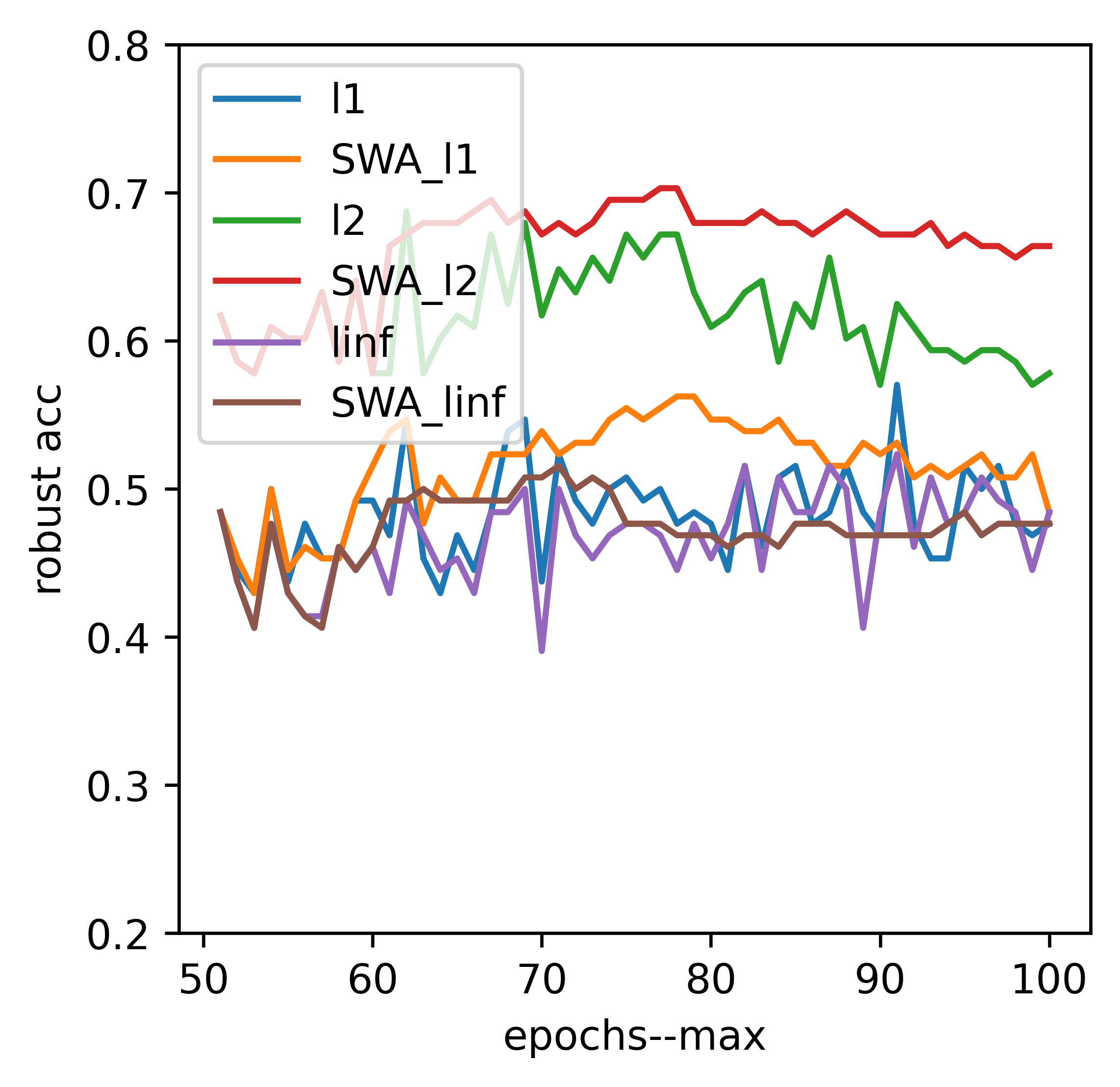
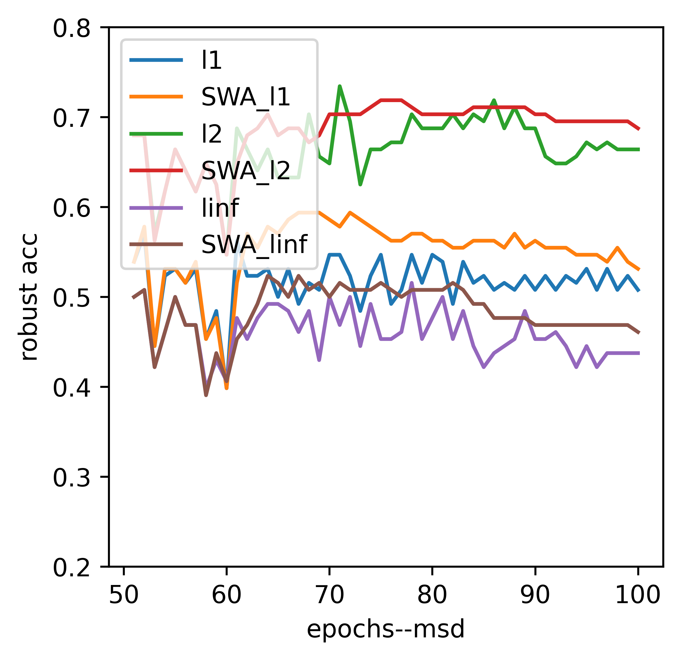
Figure 3: Tendency curves of robust accuracy against different types of adversarial attacks. The models are trained by ATMP using four different strategies, with and without SWA.

7 Conclusion

In this paper, we try to find out the difficulty of adversarial training for multiple perturbations from the perspective of optimization. Specifically, we study the smoothness of the loss function of ATMP and provide a stability analysis. Based on the analysis, we propose adaptive smoothness-weighted adversarial training for multiple perturbations, which achieve better generalization bound and achieve state-of-the-art performance against multiple perturbations.

Appendix A Proof of Theorem

In this section, we provide the detailed proof.

A.1 Proof of Proposition 4.1

Since

$$\|({\bm{X}}+\delta)\theta-y\|^{2}$$

$$\leq [\|{\bm{X}}\theta-y\|+\|\delta\theta\|]^{2}$$

$$= [\|{\bm{X}}\theta-y\|+\sqrt{\sum|\delta_{i}\theta|^{2}}]^{2}$$

$$\leq [\|{\bm{X}}\theta-y\|+\sqrt{\sum[\|\delta_{i}\|_{p}\|\theta\|_{p*}]^{2}}]^{2}$$

$$\leq [\|{\bm{X}}\theta-y\|+\sqrt{n\epsilon_{p}^{2}\|\theta\|_{p*}^{2}}]^{2}$$

$$= [\|{\bm{X}}\theta-y\|_{2}+\sqrt{n}\epsilon_{p}\|\theta\|_{p^{*}}]^{2},$$

where the first inequality is due to triangle inequality, the second inequality is due to Cauchy-Schwarz inequality, and the last inequality is due to the constraint $\|\delta\|_{p,\infty}\leq\epsilon_{p}$. Choosing $\delta_{i}$ to satisfy the aforementioned three inequalities, we obtain

$$R_{S}^{p}(\theta)=\max_{\|\delta\|_{p,\infty}\leq\epsilon_{p}}\|({\bm{X}}+\delta)\theta-y\|^{2}=[\|{\bm{X}}\theta-y\|_{2}+\sqrt{n}\epsilon_{p}\|\theta\|_{p^{*}}]^{2}.$$

Based on this, we directly have

$$R_{S}^{wst}(\theta) = \max_{p\in\{1,2,\infty\}}\max_{\|\delta\|_{p,\infty}\leq\epsilon_{p}}\|({\bm{X}}+\delta)\theta-y\|^{2}$$

$$= \max_{p\in\{1,2,\infty\}}[\|{\bm{X}}\theta-y\|_{2}+\sqrt{n}\epsilon_{p}\|\theta\|_{p^{*}}]^{2},$$

$$R_{S}^{avg}(\theta) = \mathbb{E}_{p\in\{1,2,\infty\}}\max_{\|\delta\|_{p,\infty}\leq\epsilon_{p}}\|({\bm{X}}+\delta)\theta-y\|^{2}$$

$$= \mathbb{E}_{p\in\{1,2,\infty\}}[\|{\bm{X}}\theta-y\|_{2}+\sqrt{n}\epsilon_{p}\|\theta\|_{p^{*}}]^{2}.$$

∎

A.2 Proof of Lemma 4.1

Proof:
Case 1: $\text{st}\in\{1,2,\infty\}$. The proof can be found in (Sinha et al.,, 2017; Wang et al.,, 2019).
Case 2: $\text{st}=wst$. Since $g(\theta,z)$ is locally $\mu_{p}$-strongly concave for all $z\in\mathcal{Z}$ in $\ell_{p}$-norm, $g(\theta,z)$ is locally $\min\mu_{p}$-strongly concave within the union of $\ell_{p}$ norm ball for all $z\in\mathcal{Z}$.
Case 3: $\text{st}=avg$. Since $h^{avg}(\theta,z)=\mathcal{E}h^{p}(\theta,z)$, we have

$$\|\nabla_{\theta}h^{avg}(\theta_{1},z)-\nabla_{\theta}h^{avg}(\theta_{2},z)\|=\|\mathbb{E}(\nabla_{\theta}h^{p}(\theta_{1},z)-\nabla_{\theta}h^{p}(\theta_{2},z))\|\leq\mathbb{E}\beta_{p}\|\theta_{1}-\theta_{2}\|.$$

∎

A.3 Discussion on Non-Strongly-Convex Cases

Assumption A.1.

The function $g$ satisfies the following Lipschitzian smoothness conditions:

$$\|g(\theta_{1},z)-g(\theta_{2},z)\|\leq L\|\theta_{1}-\theta_{2}\|,$$

$$\|\nabla_{\theta}g(\theta_{1},z)-\nabla_{\theta}g(\theta_{2},z)\|\leq L_{\theta}\|\theta_{1}-\theta_{2}\|,$$

$$\|\nabla_{\theta}g(\theta,z_{1})-\nabla_{\theta}g(\theta,z_{2})\|\leq L_{\theta z}^{p}\|z_{1}-z_{2}\|_{p},$$

$$\|\nabla_{z}g(\theta_{1},z)-\nabla_{\theta}g(\theta_{2},z)\|\leq L_{z\theta}\|\theta_{1}-\theta_{2}\|.$$

Assumption A.1 assumes that the gradient Lipschitz in different $\ell_{p}$-norm are $L_{\theta z}^{p}$, which can be verified by the relation between norms.

Lemma A.1.

Under Assumption A.1, $\forall\theta_{1},\theta_{2}$ and $\forall z\in\mathcal{Z}$, the following properties hold.

1. (Lipschitz function.) $\|h^{st}(\theta_{1},z)-h^{st}(\theta_{2},z)\|\leq L\|\theta_{1}-\theta_{2}\|$.

2. (Non-gradient Lipschitz.) $\|\nabla_{\theta}h^{st}(\theta_{1},z)-\nabla_{\theta}h^{st}(\theta_{2},z)\|\leq L_{\theta}\|\theta_{1}-\theta_{2}\|+\eta_{st}$, where $\eta_{p}=2L_{\theta z}^{p}\epsilon_{p}$, $\eta_{wst}=2\max\{L_{\theta z}^{p}\epsilon_{p}\}$, and $\eta_{avg}=2\mathbb{E}_{p}L_{\theta z}^{p}\epsilon_{p}$.

Lemma A.1.0 and 4.1.0 show that adversarial surrogate loss in different $\ell_{p}$ adversaries have different smoothness in general non-concave case.

Proof: Notice that $R_{S}^{st}(\theta)=\sum_{i=1}^{n}h^{st}(\theta,z_{i})/n$, we only need to prove that $\forall{\bm{x}}$, we have

$$\|h^{st}(\theta_{1},z)-h^{st}(\theta_{1},z)\|\leq L_{\theta}\|\theta_{1}-\theta_{2}\|,$$ (A.1)

$$\|\nabla_{\theta}h^{st}(\theta_{1},z)-\nabla_{\theta}h^{st}(\theta_{2},z)\|\leq L_{\theta\theta}\|\theta_{1}-\theta_{2}\|+\eta_{st},$$

where $\text{st}\in\{1,2,\infty,\text{wst},\text{avg}\}$ with $\eta_{p}=2L_{\theta{\bm{x}}}^{p}\epsilon_{p}$, $\eta_{wst}=2\max\{L_{\theta{\bm{x}}}^{p}\epsilon_{p}\}$, and $\eta_{avg}=2\mathbb{E}_{p}L_{\theta{\bm{x}}}^{p}\epsilon_{p}$.

Case 1: $\text{st}\in\{1,2,\infty\}$:

Let the adversarial examples for parameter $\theta_{1}$ and $\theta_{2}$ be

$${\bm{x}}_{1}=\arg\max_{\|\delta\|\leq\epsilon_{p}}g({\bm{x}}+\delta,\theta_{1})$$

$${\bm{x}}_{2}=\arg\max_{\|\delta\|\leq\epsilon_{p}}g({\bm{x}}+\delta,\theta_{2}),$$

then we have

$$\|h^{st}(\theta_{1},z)-h^{st}(\theta_{1},z)\|$$

$$= |g(\theta_{1},z_{1})-g(\theta_{2},z_{2})|$$

$$\leq \max\{|g(\theta_{1},z_{1})-g(\theta_{2},z_{1})|,|g(\theta_{1},z_{2})-g(\theta_{2},z_{2})|\}$$

$$\leq L_{\theta}\|\theta_{1}-\theta_{2}\|,$$

where the first inequality is based on the fact that $g(\theta_{1},z_{1})\geq g(\theta_{1},z_{2})$ and $g(\theta_{2},z_{2})\geq g(\theta_{2},z_{1})$, the second inequality is based on Assumption 1A.1. This proves the first inequality in equation (A.1) in this case. For the second one in equation (A.1), we have

$$\|\nabla_{\theta}h^{st}(\theta_{1},z)-\nabla_{\theta}h^{st}(\theta_{2},z)\|$$

$$= \|\nabla_{\theta}h^{st}(\theta_{1},z_{1})-\nabla_{\theta}g(\theta_{2},z_{2})\|$$

$$\leq \|\nabla_{\theta}h^{st}(\theta_{1},z_{1})-\nabla_{\theta}g(\theta_{2},z_{1})\|+\|\nabla_{\theta}g(\theta_{2},z_{1})-\nabla_{\theta}g(\theta_{2},z_{2})\|$$

$$\leq L_{\theta\theta}\|\theta_{1}-\theta_{2}\|+L_{\theta{\bm{x}}}^{p}\|z_{1}-z_{2}\|_{p}$$

$$\leq L_{\theta\theta}\|\theta_{1}-\theta_{2}\|+L_{\theta{\bm{x}}}^{p}[\|z_{1}-z\|_{p}+\|z-z_{2}\|_{p}]$$

$$\leq L_{\theta\theta}\|\theta_{1}-\theta_{2}\|+2L_{\theta{\bm{x}}}^{p}\epsilon_{p}$$

$$= L_{\theta\theta}\|\theta_{1}-\theta_{2}\|+\eta_{st},$$

where the first and the third inequality is triangle inequality, the second inequality is based on Assumption 1. This proves the second inequality.

Case 2: $\text{st}=\textbf{wst}$:

Let the adversarial examples for parameter $\theta_{1}$ and $\theta_{2}$ be

$${\bm{x}}_{1}=\arg\max_{p\in\{1,2,\infty\}}\max_{\|\delta\|\leq\epsilon_{p}}g({\bm{x}}+\delta,\theta_{1})$$

$${\bm{x}}_{2}=\arg\max_{p\in\{1,2,\infty\}}\max_{\|\delta\|\leq\epsilon_{p}}g({\bm{x}}+\delta,\theta_{2}),$$

the prove of the first inequality in equation (A.1) is the same as the proof in Case 1. For the second inequality in equation (A.1), we have

$$\|\nabla_{\theta}h^{st}(\theta_{1},z)-\nabla_{\theta}h^{st}(\theta_{2},z)\|$$

$$\leq L_{\theta\theta}\|\theta_{1}-\theta_{2}\|+L_{\theta{\bm{x}}}^{p}[\|z_{1}-z\|_{p}+\|z-z_{2}\|_{p}]$$

$$\leq L_{\theta\theta}\|\theta_{1}-\theta_{2}\|+2\max_{p\in\{1,2,\infty\}}[L_{\theta{\bm{x}}}^{p}\epsilon_{p}]$$

$$= L_{\theta\theta}\|\theta_{1}-\theta_{2}\|+\eta_{st}.$$

This proves the second inequality.

Case 3: $\text{st}=\textbf{avg}$:

Let the adversarial examples for parameter $\theta_{1}$ and $\theta_{2}$ and $p=1,2,\infty$ be

$${\bm{x}}_{1}^{p}=\arg\max_{\|\delta\|\leq\epsilon_{p}}g({\bm{x}}+\delta,\theta_{1})$$

$${\bm{x}}_{2}^{p}=\arg\max_{\|\delta\|\leq\epsilon_{p}}g({\bm{x}}+\delta,\theta_{2}).$$

For the first inequality in equation (A.1), we have

$$\|h^{st}(\theta_{1},z)-h^{st}(\theta_{1},z)\|$$

$$= |\mathbb{E}_{p\sim\{1,2,\infty\}}g({\bm{x}}_{1}^{p},\theta_{1})-\mathbb{E}_{p\sim\{1,2,\infty\}}g({\bm{x}}_{2}^{p},\theta_{2})|$$

$$\leq \mathbb{E}_{p\sim\{1,2,\infty\}}|g({\bm{x}}_{1}^{p},\theta_{1})-g({\bm{x}}_{2}^{p},\theta_{2})|$$

$$\leq \mathbb{E}_{p\sim\{1,2,\infty\}}\max\{|g({\bm{x}}_{1}^{p},\theta_{1})-g({\bm{x}}_{1}^{p},\theta_{2})|,|g({\bm{x}}_{2}^{p},\theta_{1})-g({\bm{x}}_{2}^{p},\theta_{2})|\}$$

$$\leq \mathbb{E}_{p\sim\{1,2,\infty\}}L_{\theta}\|\theta_{1}-\theta_{2}\|$$

$$\leq L_{\theta}\|\theta_{1}-\theta_{2}\|,$$

where the first inequality is Jensen’s inequality. This proves of the first inequality in equation (A.1) in this case. For the second inequality in equation (A.1), we have

$$\|\nabla_{\theta}h^{st}(\theta_{1},z)-\nabla_{\theta}h^{st}(\theta_{2},z)\|$$

$$= \|\nabla_{\theta}\mathbb{E}_{p\sim\{1,2,\infty\}}g({\bm{x}}_{1}^{p},\theta_{1})-\nabla_{\theta}\mathbb{E}_{p\sim\{1,2,\infty\}}g({\bm{x}}_{2}^{p},\theta_{2})\|$$

$$\leq \mathbb{E}_{p\sim\{1,2,\infty\}}\|\nabla_{\theta}g({\bm{x}}_{1}^{p},\theta_{1})-\nabla_{\theta}g({\bm{x}}_{2}^{p},\theta_{2})\|$$

$$\leq \mathbb{E}_{p\sim\{1,2,\infty\}}[L_{\theta\theta}\|\theta_{1}-\theta_{2}\|+2L_{\theta{\bm{x}}}^{p}\epsilon_{p}]$$

$$= L_{\theta\theta}\|\theta_{1}-\theta_{2}\|+\eta_{st},$$

where the first inequality is the Jensen’s inequality, the second one is the result in Case 1. the This proves the second inequality in equation (A.1) in this case.∎

A.4 Proof of Lemma 5.1

$$\|G_{z}(\theta_{1})-G_{z}(\theta_{2})\| =\|\theta_{1}-\theta_{2}-\frac{1}{P}\sum_{p=1}^{P}\alpha^{p}h^{p}(\theta_{1},z)+\frac{1}{P}\sum_{p=1}^{P}\alpha^{p}h^{p}(\theta_{2},z)\|$$

$$\leq\frac{1}{P}\sum_{p=1}^{P}\|\theta_{1}-\theta_{2}-\alpha^{p}h^{p}(\theta_{1},z)+\alpha^{p}h^{p}(\theta_{2},z)\|$$

$$\leq\frac{1}{P}\sum_{p=1}^{P}\|\theta_{1}-\theta_{2}\|$$

$$=\|\theta_{1}-\theta_{2}\|,$$

where the first inequality is due to triangular inequality, the second inequality is due to the co-coercive propertiy of convex function.∎

A.5 Proof of Theorem 5.2

To bound the generalization gap of a model, we employ the following notion of uniform stability.

Definition A.1.

A randomized algorithm $A$ is $\varepsilon$-uniformly stable if for all data sets $S,S^{\prime}\in\mathcal{Z}^{n}$ such that $S$ and $S^{\prime}$ differ in at most one example, we have

$$\sup_{z}\operatorname{\mathbb{E}}_{A}\left[h(A(S);z)-h(A(S^{\prime});z)\right]\leq\varepsilon\,.$$ (A.2)

Here, the expectation is taken over the randomness of $A$. Uniform stability implies generalization in expectation (Hardt et al.,, 2016).

Theorem A.1 (Generalization in expectation).

Let $A$ be $\varepsilon$-uniformly stable. Then, the expected generalization gap satisfies

$$|\mathcal{E}_{gen}|=\left|\operatorname{\mathbb{E}}_{S,A}[R_{\cal D}[A(S)]-R_{S}[A(S)]]\right|\leq\varepsilon\,.$$

Let $S$ and $S^{\prime}$ be two samples of size $n$ differing in only a single example. Consider two trajectories $\theta_{1}^{1},\dots,\theta_{1}^{T}$ and $\theta_{2}^{1},\dots,\theta_{2}^{T}$ induced by running an algorithm on sample $S$ and $S^{\prime},$ respectively. Let $\delta_{t}=\|\theta_{1}^{t}-\theta_{2}^{t}\|$.

Fixing an example $z\in Z$ and apply the Lipschitz condition on $h(\cdot\,;z)$, we have

$$\operatorname{\mathbb{E}}\left|h(\theta_{1}^{T};z)-h(\theta_{2}^{T};z)\right|\leq L\operatorname{\mathbb{E}}\left[\delta_{T}\right]\,.$$ (A.3)

Observe that at step $t,$ with probability $1-1/n,$ the example selected by the randomized algorithms is the same in both $S$ and $S^{\prime}.$ With probability $1/n$ the selected example is different. Based on Lemma 5.1, we have

$$\operatorname{\mathbb{E}}\left[\delta_{t+1}\right] \leq\left(1-\frac{1}{n}\right)\bigg{(}\operatorname{\mathbb{E}}[\delta_{t}]\bigg{)}+\frac{1}{n}\operatorname{\mathbb{E}}\left[\delta_{t}\right]+\frac{2\frac{1}{P}\sum_{p=1}^{P}\alpha_{t}^{p}L}{n}$$ (A.4)

$$\leq\operatorname{\mathbb{E}}\left[\delta_{t}\right]+\bigg{(}\eta+\frac{2L}{n}\bigg{)}\frac{1}{P}\sum_{p=1}^{P}\alpha_{t}^{p}\,.$$ (A.5)

Unraveling the recursion, we have

$$\operatorname{\mathbb{E}}\left[\delta_{T}\right]\leq\bigg{(}\frac{2L}{n}\bigg{)}\sum_{t=1}^{T}\frac{1}{P}\sum_{p=1}^{P}\alpha_{t}^{p},\ \text{and}\ \ \mathcal{E}_{gen}\leq L\bigg{(}\frac{2L}{n}\bigg{)}\sum_{t=1}^{T}\frac{1}{P}\sum_{p=1}^{P}\alpha_{t}^{p}\,.$$

Since this bounds holds for all $S,S^{\prime}$ and $z,$ we obtain the desired bound on the uniform stability.∎

A.6 Proof of Theorem 5.3

$$\|\theta^{t+1}-\theta^{*}\|^{2}=\bigg{\|}\theta^{t}-\theta^{*}-\frac{1}{P}\sum_{p=1}^{P}\alpha_{p}^{t}\nabla h^{p}(\theta^{t},z)\bigg{\|}^{2}$$

$$= \|\theta^{t}-\theta^{*}\|^{2}+\bigg{\|}\frac{1}{P}\sum_{p=1}^{P}\alpha_{p}^{t}\nabla h^{p}(\theta^{t},z)\bigg{\|}^{2}-2\bigg{\langle}\frac{1}{P}\sum_{p=1}^{P}\alpha_{p}^{t}\nabla h^{p}(\theta^{t},z),\theta^{t+1}-\theta^{*}\bigg{\rangle}.$$

Take expectation over $z$, we have

$$\mathbb{E}\|\theta^{t+1}-\theta^{*}\|^{2}$$

$$\leq \mathbb{E}\|\theta^{t}-\theta^{*}\|^{2}+\bigg{(}\frac{1}{P}\sum_{p=1}^{P}\alpha_{p}^{t}L\bigg{)}^{2}-\frac{2}{P}\sum_{p=1}^{P}\alpha_{p}^{t}\mathbb{E}[h^{p}(\theta^{t})-h^{p}(\theta^{*})],$$

Then,

$$\alpha_{sw}^{t}\frac{2}{P}\sum_{p=1}^{P}\mathbb{E}[h^{p}(\theta^{t})-h^{p}(\theta^{*})]\leq\mathbb{E}\|\theta^{t}-\theta^{*}\|^{2}-\mathbb{E}\|\theta^{t+1}-\theta^{*}\|^{2}$$

$$+(\alpha_{sw}^{t}L)^{2}+\frac{2}{P}\sum_{p=1}^{P}(\alpha_{sw}^{t}-\alpha_{p}^{t})\mathbb{E}[h^{p}(\theta^{t})-h^{p}(\theta^{*})]$$

Considering constant step size and expand the recursive, we have

$$T\alpha_{sw}\frac{2}{P}\sum_{p=1}^{P}\mathbb{E}[h^{p}(\theta^{T})-h^{p}(\theta^{*})]$$

$$\leq \mathbb{E}\|\theta^{T}-\theta^{*}\|^{2}+T(\alpha_{sw}L)^{2}+\frac{2T}{P}\sum_{p=1}^{P}|\alpha_{sw}^{t}-\alpha_{p}^{t}|B.$$

Therefore, we obtain the optimization error bound

$$\mathcal{E}_{opt}\leq\frac{D^{2}+L^{2}T\alpha_{sw}^{2}}{2T\alpha_{sw}}+B\frac{\sum_{p=1}^{P}|\alpha_{sw}-\alpha_{p}|}{\alpha_{sw}}.$$

∎

Appendix B Additional Experiments

In this section, the test accuracy are evaluated using the first batch (128 samples) to save the computational cost.

B.1 Gradient Norm Analysis

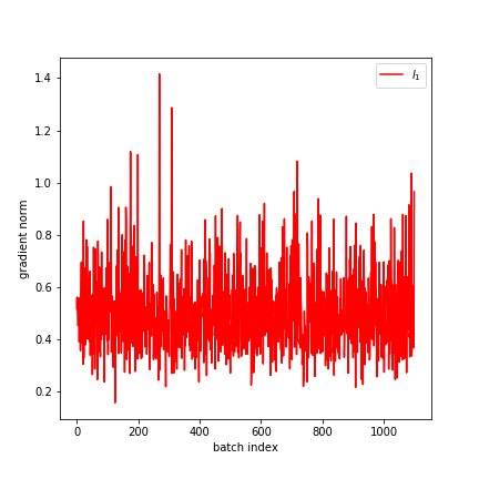
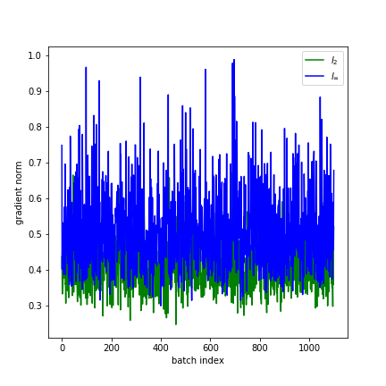
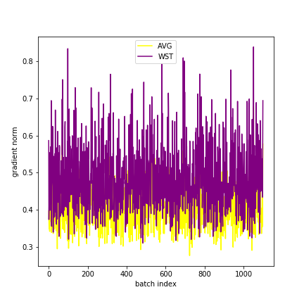
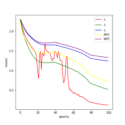
Figure 4: Gradient norms and loss value of adversarial training for single and multiple perturbations. (a) $\|\nabla R_{S}^{1}(\theta)\|$, last 1173 batch. (b) $\|\nabla R_{S}^{2}(\theta)\|$ (green) and $\|\nabla R_{S}^{\infty}(\theta)\|$ (blue), last 1173 batch. (c) $\|\nabla R_{S}^{avg}(\theta)\|$ (yellow) and $\|\nabla R_{S}^{wst}(\theta)\|$ (purple), last 1173 batch. (d) Training loss for the total 100 epochs.

Since the gradient Lipschitz $L_{\theta x}^{p}$ is unknown in practice, we provide a numerical simulation of the convergence error in this subsection on CIFAR-10 to help justify our Theoretical results. In Fig. 4, we show the gradient norm $\|\nabla R_{S}^{st}(\theta)\|$ of the last layer for the last 3 epochs ($3\times 391=1173$ batchs) for $st\in\{1,2,\infty,avg,wst\}$ as well as the training loss for the total 100 epochs.

Comparison of $\ell_{1}$, $\ell_{2}$, and $\ell_{\infty}$

In Fig. 4, We can see that $\|\nabla R_{S}^{1}(\theta)\|$ is the largest one accompany with the largest variance among these three. In (d), the training loss of $R_{S}^{1}(\theta)$ is unstable. It is because the top-k $\ell_{1}$ attack is inefficient and sparse (Tramèr and Boneh,, 2019). In the middle stage, the fluctuation is large since the success rate of the top-k attack is small. In the final stage, the top-k attack cannot find adversarial examples. Therefore, the loss is small. Comparing the $R_{S}^{2}(\theta)$ and $R_{S}^{\infty}(\theta)$, we can see that $\ell_{\infty}$ adversarial training has higher gradient norm and larger training loss. In conclusion, $\ell_{1}$ and $\ell_{\infty}$ give less contributions to the smoothness of ATMP.

B.2 Ablation Study of SWA

We give more ablation study of SWA in this subsection.

SWA on CIFAR-100

In Fig. 5, we we plots the robust accuracy of of ATMP using AVG, SAT, MAX, and MSD respectively on CIFAR-100, which are the same experiments we show in Figure 3. From the plots, we observe that without SWA, the test accuracy are highly unstable among different training epochs. There exists a trade-off between different types of adversaries. The increase in robust accuracy against one kind of adversaries may accompany with the decrease in robust accuracy on another adversarial examples. On the other side, when coupling with SWA, the tendency curves of all four ATMP strategies are largely stabilized. Besides, SWA (red, orange, and brown line) will increase the test accuracy in most of the case. The experiments in Figure 5 give the same conclusion as that of Figure 3 in the main paper.

Gradient norm of SWA

In Figure 6, we show the gradient norm of all the batches with and without SWA using AVG and MAX. On training set, the gradient norm with and without SWA is similar. On test set, the gradient norm of using SWA is smaller than that without SWA. This proves that SWA can find flatter minima with smaller gradient norm, and have better generalization.

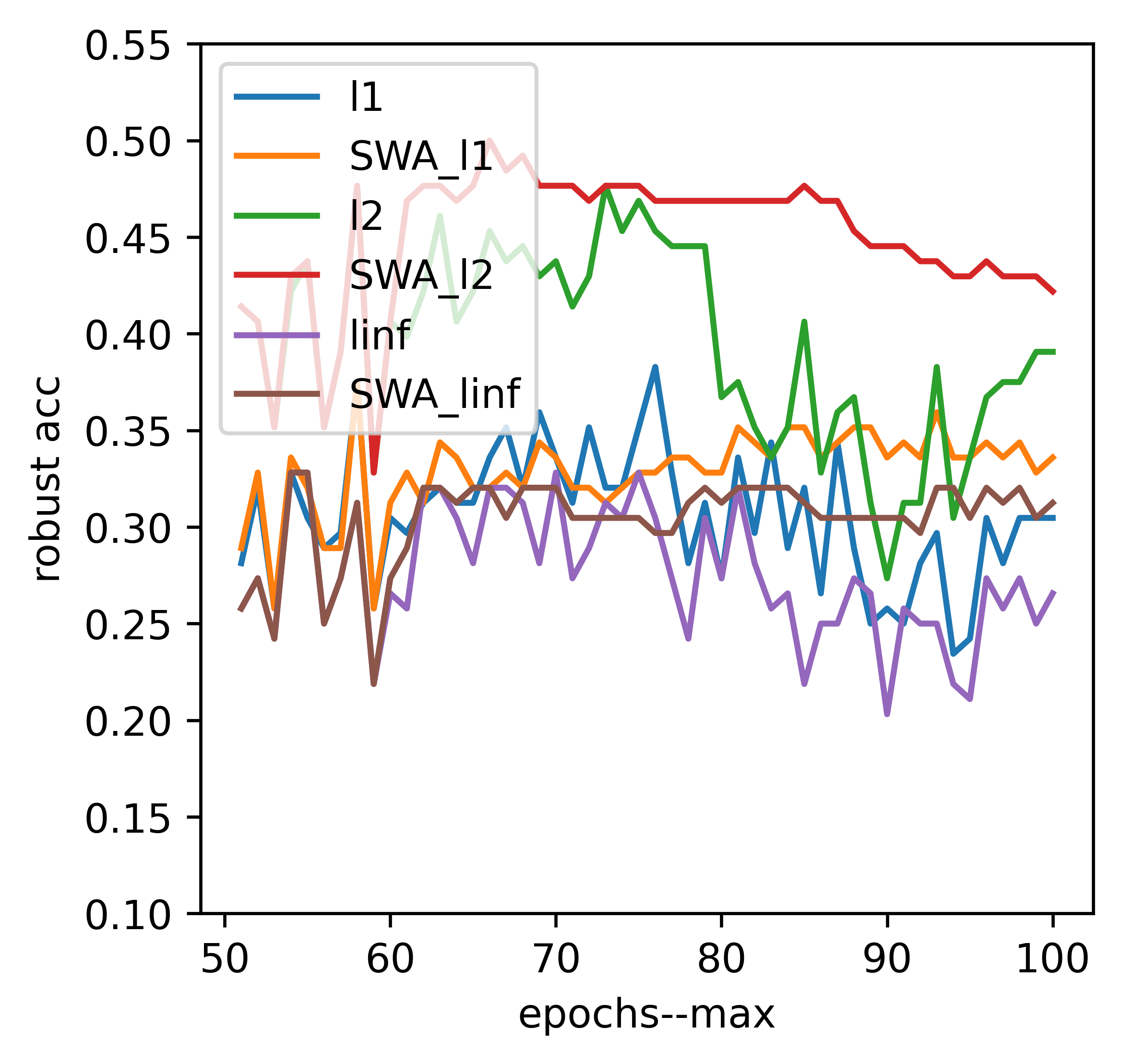
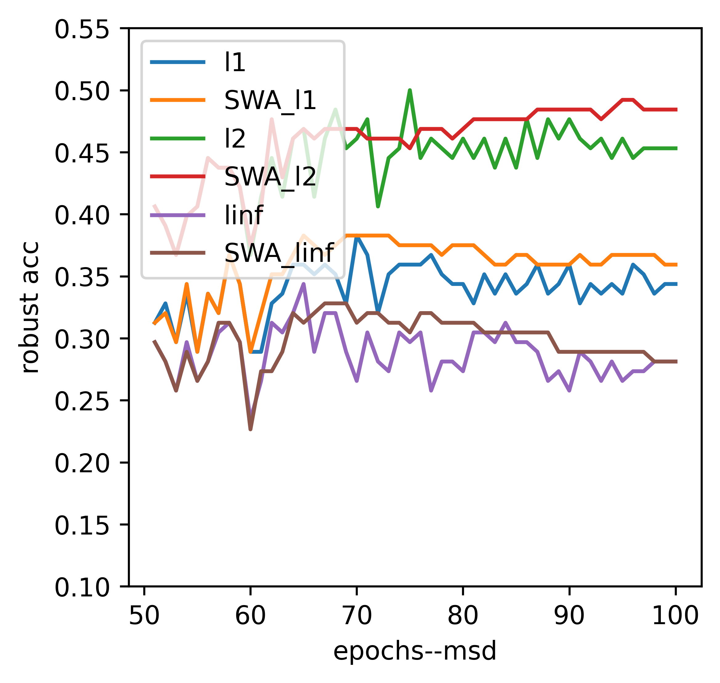
Figure 5: Results of robust accuracy for each type perturbation over epochs of multiple perturbation AT in CIFAR-100 dataset:(a) Avg and Avg-SWA, (b) SAT and SAT-SWA, (c) Max and Max-SWA, (d) MSD and MSD-SWA.

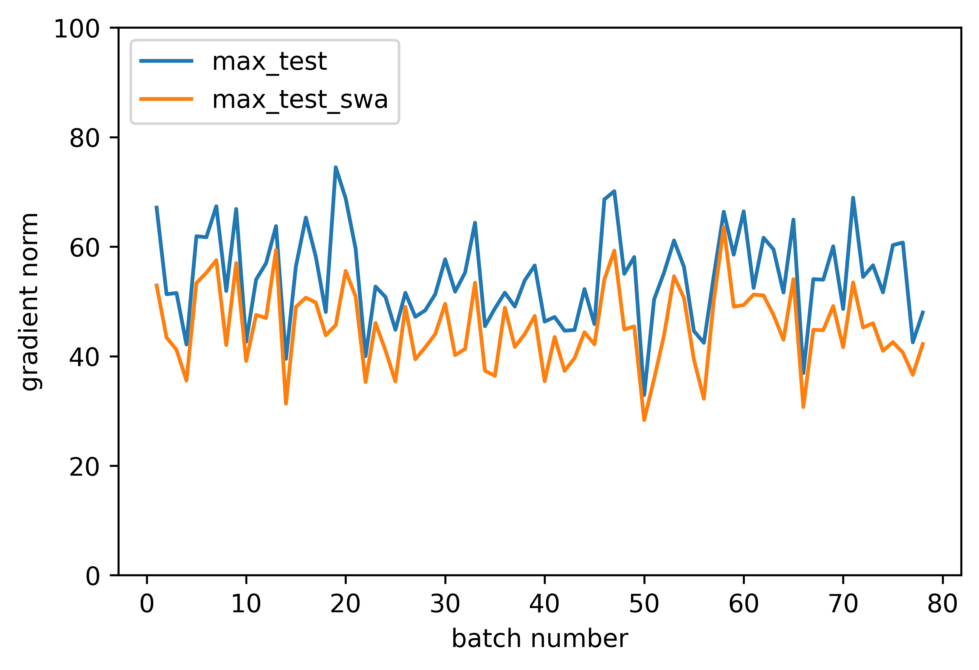
Figure 6: Gradient norm with and without SWA.

When to start SWA

In Table 3 we try to start SWA at the 60th, 70th, and 80th epochs. We use MSD for our experiments. We can see that the test accuracy against $\ell_{\infty}$ attack is higher when we start later. BUt the test accuracy against $\ell_{1}$ attack is higher when we start earlier. It is hard to say which is better but using SWA is always better than no SWA. The accuracy of AVG, MAX MSD, and SAT with and without SWA are provided in Table B.2.

Table 3: Test accuracy (%) of MSD with SWA started from the 60th,70th, and 80th epochs.

Dataset		CIFAR-10
Attack methods		clean	$\ell_{1}$	$\ell_{2}$	$\ell_{\infty}$
MSD with SWA	no SWA	83.51	50.78	66.41	43.75
	the 60th epochs	81.99	53.12	68.75	46.09
	the 70th epochs	82.01	49.22	69.53	47.66
	the 80th epochs	81.95	50.78	69.54	48.44

Table 4: Test accuracy (%) of different algorithms (MAX, AVG, MSD and SAT, with and without SWA) against $\ell_{1}$, $\ell_{2}$, and $\ell_{\infty}$ attacks on CIFAR-10 and CIFAR-100.

Dataset		CIFAR-10				CIFAR-100
Attack methods		clean	$\ell_{1}$	$\ell_{2}$	$\ell_{\infty}$	clean	$\ell_{1}$	$\ell_{2}$	$\ell_{\infty}$
AT	$\ell_{1}$	93.19	89.84	0.00	0.00	70.98	73.44	00.78	00.78
	$\ell_{2}$	88.66	41.41	61.72	39.84	63.76	21.88	43.75	20.31
	$\ell_{\infty}$	84.94	17.19	53.91	46.88	58.86	11.72	39.06	30.47
ATMP	AVG	85.28	50.78	64.84	38.28	59.71	39.84	47.66	21.88
	MAX	84.96	43.75	49.22	41.41	57.90	30.47	39.06	26.56
	MSD	83.51	50.78	66.41	43.75	57.33	34.38	45.31	28.12
	SAT	85.23	53.12	69.53	40.62	59.25	39.84	42.97	28.12
ATMP with SWA	AVG	83.19	57.03	69.53	42.97	58.04	40.62	48.44	28.12
	MAX	83.78	42.19	60.16	47.66	58.29	33.59	42.19	31.25
	MSD	81.99	53.12	68.75	46.09	57.33	35.94	48.44	28.12
	SAT	84.76	59.38	71.09	42.97	60.18	39.84	45.31	28.12

B.3 Other Tricks

Label smoothing (LS)

Label smoothing is introduced as regularization to improve generalization by replacing the one-hot labels to soft labels in the cross-entropy loss. It is shown that it relates to flat minima and yields better generalization. In the cross-entropy loss, using soft labels other than one-hot label can increase the smoothness of the loss function. Given probability $\gamma\in[0,1]$ and number of classes $K$, for each sample $({\bm{x}}_{i},y_{i})$, let $y_{i}$ keeps the true label with probability $1-\gamma$, $y_{i}$ is replace by a wrong label in one of the other $K-1$ classes with equal probability $\gamma/(K-1)$. The performance of ATMP with label smoothing is provided in Table B.3. We can see that label smoothing provides some improvement in these four strategies.

Table 5: Test accuracy (%) of different algorithms (MAX, AVG, MSD and SAT, with label smoothing) against $\ell_{1}$, $\ell_{2}$, and $\ell_{\infty}$ attacks on CIFAR-10 and CIFAR-100.

Dataset		CIFAR-10				CIFAR-100
Attack methods		clean	$\ell_{1}$	$\ell_{2}$	$\ell_{\infty}$	clean	$\ell_{1}$	$\ell_{2}$	$\ell_{\infty}$
ATMP with LS	AVG	85.57	55.47	68.75	39.06	60.58	38.28	46.88	24.22
	MAX	84.49	45.31	57.03	45.31	58.25	33.59	45.31	29.69
	MSD	83.49	50.78	69.53	45.30	58.61	35.94	48.44	32.03
	SAT	85.70	53.91	67.97	37.50	60.17	39.84	44.53	26.56
ATMP with LS & SWA	AVG	83.42	57.03	71.09	48.44	59.09	42.19	45.31	28.12
	MAX	83.05	47.66	63.28	46.09	57.76	39.84	47.66	31.25
	MSD	82.15	50.78	71.88	46.09	57.70	38.28	46.88	35.94
	SAT	84.96	56.25	66.41	41.41	60.51	39.06	47.66	29.69

Label noise

Label noise is a alternative choose of label smoothing. Given probability $\gamma\in[0,1]$ and number of classes $K$, for each sample $({\bm{x}}_{i},y_{i})$, let $y_{i}$ keeps the true label with probability $1-\gamma$, $y_{i}$ is replace by a wrong label in one of the other $K-1$ classes with equal probability $\gamma/(K-1)$. The difference between label noise and label smoothing is that label noise use hard label while label smoothing use soft label.

In Table 6, we provide the experiments of incorporating label noise in ATMP. We can see that label noise can give some improvements. But the improvements are not comparable to label smoothing. The reason behind is that label noise cannot increase the smoothness of the loss function of ATMP.

Table 6: Test accuracy (%) of ATMP with label noise.

Dataset		CIFAR-10
Attack methods		clean	$\ell_{1}$	$\ell_{2}$	$\ell_{\infty}$
ATMP with LN	MAX	84.18	43.75	57.03	44.53
	AVG	84.67	57.03	70.31	41.41
	MSD	82.79	52.34	6562	47.66
	SAT	85.36	56.25	69.53	42.19
ATMP with LN & SWA	MAX	81.66	50.78	63.28	47.66
	AVG	81.06	57.81	70.31	42.97
	MSD	81.03	51.56	64.84	50.00
	SAT	84.00	59.38	67.19	46.88

Silu activation function

Silu activation function is proposed to deal with the non-smoothness of Relu activation function. In Table 7, we can see that Silu has some small improvement on ATMP.

Table 7: Test accuracy (%) of ATMP with Silu activation function.

Dataset		CIFAR-10
Attack methods		clean	$\ell_{1}$	$\ell_{2}$	$\ell_{\infty}$
ATMP with Silu	MAX	80.91	53.91	64.84	46.09
	AVG	81.61	57.03	70.31	42.19
	MSD	80.44	57.03	64.84	48.44
	SAT	83.89	54.69	64.84	44.53
ATMP with Silu & SWA	MAX	78.48	50.78	67.19	49.22
	AVG	78.20	58.59	68.75	42.98
	MSD	78.39	55.47	66.41	49.99
	SAT	82.02	57.81	67.19	45.31

Mixup

We use adversarial examples in the form ${\bm{x}}_{adv}={\bm{x}}+(\delta_{1}+\delta_{2}+\delta_{\infty})/3$ for adversarial training. In Table 8, we can see that the robust accuracy is not comparable to MAX and AVG. It is because this training procedure focuses more on the mixup adversarial examples. It fails to fit the three types of adversarial examples.

Table 8: Test accuracy (%) of ATMP using mixup.

Dataset		CIFAR-10
Attack methods		clean	$\ell_{1}$	$\ell_{2}$	$\ell_{\infty}$
Other tricks	Mixup	84.73	51.56	67.19	39.06

References

- Allen-Zhu et al., (2019) Allen-Zhu, Z., Li, Y., and Song, Z. (2019). A convergence theory for deep learning via over-parameterization. In International Conference on Machine Learning, pages 242–252. PMLR.
- Awasthi et al., (2020) Awasthi, P., Frank, N., and Mohri, M. (2020). Adversarial learning guarantees for linear hypotheses and neural networks. In International Conference on Machine Learning, pages 431–441. PMLR.
- Cheng et al., (2021) Cheng, H., Xu, K., Wang, C., Lin, X., Kailkhura, B., and Goldhahn, R. (2021). Mixture of robust experts (more): A flexible defense against multiple perturbations. arXiv preprint arXiv:2104.10586.
- Du et al., (2019) Du, S., Lee, J., Li, H., Wang, L., and Zhai, X. (2019). Gradient descent finds global minima of deep neural networks. In International Conference on Machine Learning, pages 1675–1685. PMLR.
- Gao et al., (2019) Gao, R., Cai, T., Li, H., Hsieh, C.-J., Wang, L., and Lee, J. D. (2019). Convergence of adversarial training in overparametrized neural networks. Advances in Neural Information Processing Systems, 32:13029–13040.
- Goodfellow et al., (2014) Goodfellow, I. J., Shlens, J., and Szegedy, C. (2014). Explaining and harnessing adversarial examples. arXiv preprint arXiv:1412.6572.
- Gowal et al., (2020) Gowal, S., Qin, C., Uesato, J., Mann, T., and Kohli, P. (2020). Uncovering the limits of adversarial training against norm-bounded adversarial examples. arXiv preprint arXiv:2010.03593.
- Hardt et al., (2016) Hardt, M., Recht, B., and Singer, Y. (2016). Train faster, generalize better: Stability of stochastic gradient descent. In International Conference on Machine Learning, pages 1225–1234. PMLR.
- He et al., (2016) He, K., Zhang, X., Ren, S., and Sun, J. (2016). Identity mappings in deep residual networks. In European conference on computer vision, pages 630–645. Springer.
- Izmailov et al., (2018) Izmailov, P., Podoprikhin, D., Garipov, T., Vetrov, D., and Wilson, A. G. (2018). Averaging weights leads to wider optima and better generalization. arXiv preprint arXiv:1803.05407.
- Krizhevsky et al., (2009) Krizhevsky, A., Hinton, G., et al. (2009). Learning multiple layers of features from tiny images.
- (12) Liu, A., Tang, S., Liu, X., Chen, X., Huang, L., Tu, Z., Song, D., and Tao, D. (2020a). Towards defending multiple adversarial perturbations via gated batch normalization. arXiv preprint arXiv:2012.01654.
- (13) Liu, C., Salzmann, M., Lin, T., Tomioka, R., and Süsstrunk, S. (2020b). On the loss landscape of adversarial training: Identifying challenges and how to overcome them. arXiv preprint arXiv:2006.08403.
- Madaan et al., (2020) Madaan, D., Shin, J., and Hwang, S. J. (2020). Learning to generate noise for robustness against multiple perturbations. arXiv preprint arXiv:2006.12135.
- Madry et al., (2017) Madry, A., Makelov, A., Schmidt, L., Tsipras, D., and Vladu, A. (2017). Towards deep learning models resistant to adversarial attacks. arXiv preprint arXiv:1706.06083.
- Maini et al., (2021) Maini, P., Chen, X., Li, B., and Song, D. (2021). Perturbation type categorization for multiple $\ell_p$ bounded adversarial robustness.
- Maini et al., (2020) Maini, P., Wong, E., and Kolter, Z. (2020). Adversarial robustness against the union of multiple perturbation models. In International Conference on Machine Learning, pages 6640–6650. PMLR.
- Nandy et al., (2020) Nandy, J., Hsu, W., and Lee, M. L. (2020). Approximate manifold defense against multiple adversarial perturbations. In 2020 International Joint Conference on Neural Networks (IJCNN), pages 1–8. IEEE.
- Nemirovski et al., (2009) Nemirovski, A., Juditsky, A., Lan, G., and Shapiro, A. (2009). Robust stochastic approximation approach to stochastic programming. SIAM Journal on optimization, 19(4):1574–1609.
- Raghunathan et al., (2019) Raghunathan, A., Xie, S. M., Yang, F., Duchi, J. C., and Liang, P. (2019). Adversarial training can hurt generalization. arXiv preprint arXiv:1906.06032.
- Schmidt et al., (2018) Schmidt, L., Santurkar, S., Tsipras, D., Talwar, K., and Madry, A. (2018). Adversarially robust generalization requires more data. In Advances in Neural Information Processing Systems, pages 5014–5026.
- Sinha et al., (2017) Sinha, A., Namkoong, H., and Duchi, J. (2017). Certifiable distributional robustness with principled adversarial training. arXiv preprint arXiv:1710.10571, 2.
- Smith, (2018) Smith, L. N. (2018). A disciplined approach to neural network hyper-parameters: Part 1–learning rate, batch size, momentum, and weight decay. arXiv preprint arXiv:1803.09820.
- Stutz et al., (2020) Stutz, D., Hein, M., and Schiele, B. (2020). Confidence-calibrated adversarial training: Generalizing to unseen attacks. In International Conference on Machine Learning, pages 9155–9166. PMLR.
- Stutz et al., (2021) Stutz, D., Hein, M., and Schiele, B. (2021). Relating adversarially robust generalization to flat minima. arXiv preprint arXiv:2104.04448.
- Szegedy et al., (2013) Szegedy, C., Zaremba, W., Sutskever, I., Bruna, J., Erhan, D., Goodfellow, I., and Fergus, R. (2013). Intriguing properties of neural networks. arXiv preprint arXiv:1312.6199.
- Tramèr and Boneh, (2019) Tramèr, F. and Boneh, D. (2019). Adversarial training and robustness for multiple perturbations. In Advances in Neural Information Processing Systems, pages 5858–5868.
- Tramer et al., (2020) Tramer, F., Carlini, N., Brendel, W., and Madry, A. (2020). On adaptive attacks to adversarial example defenses. arXiv preprint arXiv:2002.08347.
- Wang et al., (2019) Wang, Y., Ma, X., Bailey, J., Yi, J., Zhou, B., and Gu, Q. (2019). On the convergence and robustness of adversarial training. In ICML, volume 1, page 2.
- Xing et al., (2021) Xing, Y., Song, Q., and Cheng, G. (2021). On the generalization properties of adversarial training. In International Conference on Artificial Intelligence and Statistics, pages 505–513. PMLR.
- Yin et al., (2019) Yin, D., Kannan, R., and Bartlett, P. (2019). Rademacher complexity for adversarially robust generalization. In International Conference on Machine Learning, pages 7085–7094. PMLR.
- Zhang et al., (2021) Zhang, X., Zhang, Z., and Wang, T. (2021). Composite adversarial training for multiple adversarial perturbations and beyond.