Symmetry group at future null infinity I :

Scalar theory

Wen-Bin Liu, Jiang Long

School of Physics, Huazhong University of Science and Technology,
Luoyu Road 1037, Wuhan, Hubei 430074, China

We reduce the massless scalar field theory in Minkowski spacetime to future null infinity. We compute the Poincaré flux operators, which can be generalized and identified as the supertranslation and superrotation generators. These generators are shown to form a closed symmetry algebra with a divergent central charge. In the classical limit, we argue that the algebra may be interpreted as the geometric symmetry of a Carrollian manifold, i.e., the hypersurface of future null infinity. Our method may be used to find more physically interesting Carrollian field theories.

1 Introduction

The detection of gravitational waves [1] opens a new window on the observation of the universe. The gravitational wave is one of the greatest predictions of Einstein’s equation. Theoretically, it has been known for a long time that the gravitational waves are radiated to future null infinity ($\mathcal{I}^{+}$) in asymptotically flat spacetime and they transform in the solution space according to the Bondi-Metzner-Sachs (BMS) group [2, 3, 4]. Classically, the BMS group is a semi-direct product of Lorentz group and supertranslations. Over the past decade, there have been various approaches on the understanding of the BMS group.

The conventional approach is the so-called asymptotic symmetry analysis. By imposing fall off boundary conditions on the solutions of the gravitational field, the BMS group consists of the large diffeomorphisms that preserve the boundary conditions. The BMS group allows various extensions by including the so-called superrotations. The Barnich-Troessaert (BT) superrotations are generated by local conformal Killing vectors of the celestial sphere [5, 6, 7, 8]. On the other hand, the Campiglia-Laddha (CL) superrotations are generated by diffeomorphisms of the celestial sphere [9, 10]. Both of them are discussed extensively in the literature.

The amplitude approach is motivated by the discovery of a set of infrared equivalences [11, 12]. Such equivalences relate the BMS asymptotic symmetries, soft theorems [13] and classical memory effects [14, 15, 16, 17]. As an attempt to apply the holographic principle to flat spacetime, the amplitude approach is to map the S-matrix to conformal correlators living on the celestial sphere [18, 19, 20, 21, 22, 23, 24].

The Carroll group approach is based on the symmetry of the Carroll manifold [25, 26, 27]. As is well known, the Galilei group could be obtained from the non-relativistic limit (the speed of light $c\to\infty$) of the Poincaré group. On the other hand, the Carroll group is the ultra-relativistic limit ($c\to 0$) of the Poincaré group, which is the dual of the Galilei group. The BMS group has been shown to be the so-called conformal Carroll group of level 2 [28, 29, 30]. From the point of view of flat holography, it would be interesting to construct field theories with Carrollian symmetry [31, 32, 33, 34, 35, 36, 37, 38].

In this work, we obtain a scalar field theory by projecting massless scalar field theory in flat spacetime to its conformal boundary $\mathcal{I}^{+}$. By imposing the fall-off condition of the scalar field near $\mathcal{I}^{+}$, we may solve the bulk equation of motion (EOM) asymptotically. There is no constraint on the radiation degree of freedom at the leading order of the EOM. Nevertheless, they form the radiation phase space and obey standard commutation relations in the sense of Ashtekar [39, 40, 41, 42]. We can define flux operators at $\mathcal{I}^{+}$ by computing the outgoing Poincaré fluxes from radiation. The energy-momentum flux operators are shown to form a Virasoro algebra. By including the angular momentum and the center-of-mass flux operators, we find a new group which may be regarded as a generalization of the Newman-Unti group of the Carroll manifold $\mathcal{I}^{+}$. In the soft limit, this new group is reduced to the BMS group.

This paper is organized as follows. In section 2 we review the BMS group and introduce the conventions used in this work. In section 3, we construct the ten Poincaré fluxes radiated to $\mathcal{I}^{+}$. We compute the commutation relations at $\mathcal{I}^{+}$ in the following section. In section 5, we compute the commutators of the flux operators and find a closed algebra. We also discuss antipodal matching condition in this section. In section 6, we obtain the same algebra by generalizing the Newman-Unti group of the Carroll manifold $\mathcal{I}^{+}$. We conclude in section 7. Several technical computations, the derivation of commutators using symplectic structure, and a review about light-ray operator formalism are relegated to four appendices.

2 Review of the formalism

In Minkowski spacetime $\mathbb{R}^{1,3}$, the metric can be written as

$$ds^{2}=-dt^{2}+dx^{i}dx^{i},\quad i=1,2,3.$$ (2.1)

To study radiation at future null infinity $\mathcal{I}^{+}$, we can use the retarded coordinate $(u,r,\theta,\phi)$

$$u=t-r,\quad r=\sqrt{\bm{x}^{2}},\quad\bm{x}=(x^{1},x^{2},x^{3}),$$ (2.2)

and write the metric as

$$ds^{2}=-du^{2}-2dudr+r^{2}d\Omega^{2},$$ (2.3)

where

$$d\Omega^{2}=d\theta^{2}+\sin^{2}\theta d\phi^{2}\equiv\gamma_{AB}d\theta^{A}d\theta^{B},\quad A,B=1,2$$ (2.4)

is the metric of the unit sphere

$$\gamma_{AB}=\left(\begin{array}[]{cc}1&0\\ 0&\sin^{2}\theta\end{array}\right).$$ (2.7)

In this paper, the covariant derivative $\nabla_{A}$ is adapted to the metric $\gamma_{AB}$. $\mathcal{I}^{+}$ can be approached by setting $r\to\infty$ while keeping $u$ fixed. It has the topology $\mathbb{R}\times S^{2}$ and can be described by three coordinates

$$(u,\theta,\phi)=(u,\theta^{A}).$$ (2.8)

In an asymptotically flat spacetime, the large-$r$ expansion of the metric near $\mathcal{I}^{+}$ is

$$ds^{2}=-du^{2}-2dudr+r^{2}\gamma_{AB}d\theta^{A}d\theta^{B}+\delta g_{\mu\nu}dx^{\mu}dx^{\nu}.$$ (2.9)

The original BMS group [2, 3] is the large diffeomorphism that preserves the Bondi gauge

$$\delta g_{rr}=\delta g_{rA}=0,\quad\partial_{r}(r^{-4}\det g_{AB})=0$$ (2.10)

and the boundary fall-off conditions

$$\delta g_{uu}=\mathcal{O}\left(\frac{1}{r}\right),\quad\delta g_{ur}=\mathcal{O}\left(\frac{1}{r^{2}}\right),\quad\delta g_{uA}=\mathcal{O}(1),\quad\delta g_{AB}=\mathcal{O}(r).$$ (2.11)

Transformations generated by the vector

$$\xi_{f}=f\partial_{u}+\frac{1}{2}\nabla_{A}\nabla^{A}f\partial_{r}-\frac{\nabla^{A}f}{r}\partial_{A}+\cdots$$ (2.12)

are called supertranslations. The function $f$ is smooth on $S^{2}$. More explicitly, we write it as

$$f=f(\Omega).$$ (2.13)

Similarly, the transformations generated by the vector

$$\xi_{Y}=\frac{1}{2}u\nabla_{A}Y^{A}\partial_{u}-\frac{1}{2}(u+r)\nabla_{A}Y^{A}\partial_{r}+(Y^{A}-\frac{u}{2r}\nabla^{A}\nabla_{B}Y^{B})\partial_{A}+\cdots$$ (2.14)

are called superrotations. We will distinguish two cases:

• The vector $Y^{A}$ is a local (singular) conformal Killing vector (CKV) on $S^{2}$. In this case, the vector $Y^{A}$ can be divided into holomorphic and anti-holomorphic parts. This is the superrotation in the BT sense. We will not consider this case in this paper.

• The vector $Y^{A}$ is smooth on $S^{2}$ and generates a diffeomorphism on $S^{2}$, namely

  $$Y^{A}=Y^{A}(\Omega).$$ (2.15)

  This is the CL superrotation.

By combining supertranslations and superrotations, the usual BMS group is generated by the vector

$$\xi_{f,Y}=Y^{A}(\Omega)\partial_{A}+[f(\Omega)+\frac{u}{2}\nabla_{A}Y^{A}(\Omega)]\partial_{u}$$ (2.16)

at future null infinity.

3 Fluxes

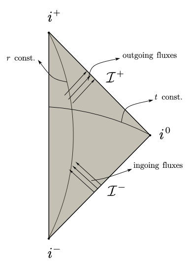
Figure 1: Penrose diagram of the Minkowski spacetime. Massive particles come from past timelike infinity $i^{-}$ and go to future timelike infinity $i^{+}$. Massless particles start from past null infinity $\mathcal{I}^{-}$ and move to future null infinity $\mathcal{I}^{+}$. $\mathcal{I}^{+}$ and $\mathcal{I}^{-}$ are null hypersurfaces with topology $\mathbb{R}\times S^{2}$. There are ingoing fluxes at $\mathcal{I}^{-}$ and outgoing fluxes at $\mathcal{I}^{+}$.

Since BMS symmetry relates to the radiation phase space at $\mathcal{I}^{+}$, we will use a massless real scalar to study the radiation at $\mathcal{I}^{+}$. The action is

$$S=\int d^{4}x[-\frac{1}{2}\partial_{\mu}\Phi\partial^{\mu}\Phi-V(\Phi)+J\Phi].$$ (3.1)

The first term is the kinematic term and the second term is the potential. Since the theory is massless, the potential is $V(\Phi)\sim\Phi^{3}$ perturbatively. To be more precisely, we may expand the potential as

$$V(\Phi)=\sum_{k=3}^{\infty}\frac{\lambda_{k}}{k}\Phi^{k}.$$ (3.2)

The last term in the action is a source coupled to the field and it causes the scalar radiation. The stress-energy tensor of the theory is

$$T_{\mu\nu}=\partial_{\mu}\Phi\partial_{\nu}\Phi+\eta_{\mu\nu}\mathcal{L},\quad\mu,\nu=0,1,2,3.$$ (3.3)

where the Lagrangian can be read out from the action (3.1).

Figure 1 is the Penrose diagram of the Minkowski spacetime. The scalar theory is in the bulk of the Penrose diagram. At the boundary, there are non-trivial outgoing fluxes at $\mathcal{I}^{+}$ and ingoing fluxes at $\mathcal{I}^{-}$. To find the radiation degree of freedom, we should reduce the field $\Phi$ to $\mathcal{I}^{+}$. This is achieved by imposing the following fall-off condition

$$\Phi = \frac{\Sigma(u,\Omega)}{r}+\sum_{k\geq 2}\frac{\Sigma^{(k)}(u,\Omega)}{r^{k}}$$ (3.4)

$$= \frac{\Sigma(u,\Omega)}{r}+\frac{\Sigma^{(2)}(u,\Omega)}{r^{2}}+\mathcal{O}\left(\frac{1}{r^{3}}\right)$$

near $\mathcal{I}^{+}$. Just as in electrodynamics [45], the field $\Sigma$ encodes the radiation degree of freedom. The fields $\Sigma^{(k)},\ k\geq 2$ are subleading terms which will be discussed in the equation of motion. The variation of the scalar field under a general diffeomorphism is

$$\delta_{\xi}\Phi=\xi^{\mu}\partial_{\mu}\Phi.$$ (3.5)

Therefore, the transformation of the boundary field $\Sigma$ under supertranslation is

$$\delta_{f}\Sigma = f\dot{\Sigma}$$ (3.6)

where $\dot{\Sigma}=\partial_{u}\Sigma$. Similarly, we find the transformation of the field $\Sigma$ under superrotation

$$\delta_{Y}\Sigma = \frac{1}{2}u\nabla_{A}Y^{A}\dot{\Sigma}+Y^{A}\nabla_{A}\Sigma+\frac{1}{2}\nabla_{A}Y^{A}\Sigma.$$ (3.7)

The first term on the right hand side of (3.7) may be subtracted, since it has the same form as the right hand side of (3.6). For the remaining two terms, we may define

$$\Delta(Y;\Sigma;u,\Omega)=Y^{A}\nabla_{A}\Sigma(u,\Omega)+\frac{1}{2}\nabla_{A}Y^{A}\Sigma(u,\Omega)$$ (3.8)

for later convenience.

From the action (3.1), the equation of motion is

$$\Box\Phi-\frac{\partial V}{\partial\Phi}+J=0.$$ (3.9)

The external source affects the vacuum state of the theory and modifies the quantum expectation value and the correlation functions of the field $\Sigma$. However, we will consider quantum fluctuations of the field around the vacuum state, so it is safe to set it to zero. From now on, we ignore the source term and try to solve the equation of motion near $\mathcal{I}^{+}$. Using the fall-off condition (3.4) and the potential (3.2), we can solve the equation of motion order by order. More explicitly, we have

$$\partial_{0}^{2}\Phi=\frac{\ddot{\Sigma}}{r}+\frac{\ddot{\Sigma}^{(2)}}{r^{2}}+\frac{\ddot{\Sigma}^{(3)}}{r^{3}}+\cdots,$$ (3.10)

and

$$\partial^{2}_{i}\Phi= \frac{\ddot{\Sigma}}{r}+\frac{\ddot{\Sigma}^{(2)}}{r^{2}}+\frac{1}{r^{3}}\bigg{[}\gamma^{AB}\nabla_{A}\nabla_{B}\Sigma+2\dot{\Sigma}^{(2)}+\ddot{\Sigma}^{(3)}\bigg{]}+\cdots.$$ (3.11)

Therefore, we could obtain the following results.

• At the leading order $\mathcal{O}(r^{-1})$, the time derivative of $\Sigma$ is cancelled out and there is no corresponding EOM for $\Sigma$. There would exist term with time derivative of $\Sigma$ from $\partial_{0}^{2}\Phi$. However, the contribution about such term from $-\partial_{0}^{2}\Phi$ exactly cancels that from $\partial_{i}^{2}\Phi$.

• At the subleading order $\mathcal{O}(r^{-2})$, we find the following equation

  $$\lambda_{3}\Sigma^{2}=0.$$ (3.12)

  From (3.12), the field $\Sigma$ should be zero when $\lambda_{3}\not=0$. To find non-trivial phase space, we may choose $\lambda_{3}=0$. Then the equation is valid without imposing any constraint on the field $\Sigma$.

• At next order $\mathcal{O}(r^{-3})$, we find

  $$-\lambda_{4}\Sigma^{3}+2\dot{\Sigma}^{(2)}+\gamma^{AB}\nabla_{A}\nabla_{B}\Sigma=0.$$ (3.13)

  The subleading term $\Sigma^{(2)}$ is determined when we impose the initial condition at the initial time $u=u_{i}$

  $$\Sigma^{(2)}(u=u_{i},\Omega)=\sigma^{(2)}(\Omega).$$ (3.14)

  The initial data $\sigma^{(2)}(\Omega)$ is independent of the field $\Sigma$. Equation (3.13) indicates that $\Sigma^{(2)}$ is not an independent propagating degree of freedom at $\mathcal{I}^{+}$.

• At higher orders $\mathcal{O}(r^{-k}),\ k\geq 4$, we can also prove that $\Sigma^{(k-1)}$ are not independent propagating degrees of freedom.

In this paper, the Poincaré fluxes could be expressed in terms of the field $\Sigma$ without any contribution from the higher order terms $\Sigma^{(k)},\ k\geq 2$. We will focus on field $\Sigma$ in the following.

3.1 Energy and momentum fluxes

To find the energy flux at $\mathcal{I}^{+}$, we use the conservation of the stress-energy tensor

$$\partial_{\mu}T^{\nu\mu}=0.$$ (3.15)

It follows that the energy flux can be written as

$$\frac{dP^{0}}{dt} = \frac{d}{dt}\int_{V}d^{3}\bm{x}T^{00}=-\int_{V}d^{3}\bm{x}\partial_{i}T^{0i}=-\int_{\partial V}dS_{i}T^{0i}.$$ (3.16)

$T^{0i}$ is the $i$-th component of the energy flux density [46] which is radiated out of surface of the volume $V$. Near $\mathcal{I}^{+}$, it is expanded as

$$T^{0i}=\frac{\dot{\Sigma}^{2}n^{i}}{r^{2}}+\mathcal{O}\left(\frac{1}{r^{3}}\right).$$ (3.17)

The leading term cancels the factor $r^{2}$ in the integration measure

$$dS_{i}=r^{2}n_{i}d\Omega$$ (3.18)

and leads to a finite result. Note that the right hand side of (3.16) is a function of $u$. In the retarded coordinates (2.2), the derivative with respect to $u$ can be found by using the chain rule,

$$\frac{d}{du}=\frac{\partial t}{\partial u}\frac{d}{dt}=\frac{d}{dt}.$$ (3.19)

Therefore, we find the energy flux

$$\frac{dP^{0}}{du}=-\int_{S^{2}}d\Omega\ \dot{\Sigma}^{2}(u,\Omega).$$ (3.20)

In a similar way, we find the following momentum flux

$$\frac{dP^{i}}{du}=-\int_{S^{2}}d\Omega\ \dot{\Sigma}^{2}(u,\Omega)n^{i},$$ (3.21)

where $n^{i}$ is the normal vector of the unit sphere $S^{2}$

$$n^{i}=(\sin\theta\cos\phi,\sin\theta\cos\phi,\cos\theta).$$ (3.22)

The energy and momentum radiated to $\mathcal{I}^{+}$ during the time $(-\infty,u_{0})$ can be written as

$$T_{f}(u_{0})=\int_{-\infty}^{u_{0}}dud\Omega f(\Omega)\dot{\Sigma}^{2},\quad-\infty<u_{0}<\infty,$$ (3.23)

where $f$ is a function on the sphere.

• When $f=-1$, (3.23) is the energy radiated to $\mathcal{I}^{+}$.

• When $f=-n^{i}$, (3.23) is the momentum radiated to $\mathcal{I}^{+}$.

• It is natural to generalize the function $f$ to be any smooth function on the sphere. As we will see later, this corresponds to the supertranslation exactly.

The energy and momentum radiated to $\mathcal{I}^{+}$ are encoded in the expression (3.23). It is easy to see that (3.23) can be naturally generalized to the following version

$$\mathcal{T}_{f}=\int_{-\infty}^{\infty}dud\Omega f(u,\Omega)\dot{\Sigma}^{2}.$$ (3.24)

Now $f$ is a function on $\mathcal{I}^{+}$. When it is a step function

$$f(u,\Omega)=\theta(u_{0}-u)g(\Omega),$$ (3.25)

$\mathcal{T}_{f}$ is equivalent to $T_{g}(u_{0})$. If we want to study the time-dependence of the radiation, it is necessary to consider this generalization. Otherwise, after averaging over time in (3.24), any time-dependent information of $\dot{\Sigma}^{2}(u,\Omega)$ will get lost.

Due to the topology of $\mathcal{I}^{+}$, the function $f(u,\Omega)$ can be expanded in the following basis

$$f(u,\Omega)=\sum_{\ell,m}\int_{-\infty}^{\infty}d\omega c_{\omega,\ell,m}f_{\omega,\ell,m},\quad f_{\omega,\ell,m}=e^{-i\omega u}Y_{\ell,m}(\Omega),$$ (3.26)

where $\omega$ is the frequency which is dual to the retarded time and $(\ell,m)$ are used to label the spherical harmonics. Therefore, (3.24) can also be labeled by three quantum numbers $(\omega,\ell,m)$

$$\mathcal{T}_{\omega,\ell,m}=\int_{-\infty}^{\infty}dud\Omega f_{\omega,\ell,m}\dot{\Sigma}^{2}.$$ (3.27)

As we will show in Appendix D, the insertion of $e^{-i\omega u}$ is also performed in the context of light-ray operator formalism. At the end of this subsection, we will define an energy flux density operator at $\mathcal{I}^{+}$

$$T(u,\Omega)=\dot{\Sigma}^{2}.$$ (3.28)

It encodes equivalent information of the smeared operator (3.24).

3.2 Angular momentum and center-of-mass fluxes

The system is also Lorentz invariant. Thus we can also find a conserved current

$$M^{\mu\nu\rho}=x^{\mu}T^{\nu\rho}-x^{\nu}T^{\mu\rho},\quad\partial_{\rho}M^{\mu\nu\rho}=0$$ (3.29)

whose corresponding conserved charges are the angular momentum and center-of-mass. Therefore, we can find the following fluxes at $\mathcal{I}^{+}$

$$\frac{dL^{\mu\nu}}{du} = -\int_{V}d^{3}\bm{x}\partial_{i}M^{\mu\nu i}=-\int_{\partial V}dS_{i}M^{\mu\nu i}.$$ (3.30)

• For the rotation symmetry, we find the angular momentum fluxes

  $$\frac{dL^{ij}}{du} = \int_{S^{2}}d\Omega Y_{ij}^{A}\ \dot{\Sigma}\nabla_{A}\Sigma,$$ (3.31)

  where $Y_{ij}^{A}$ are the three Killing vectors of $S^{2}$

  $$Y_{12}^{A} = (0,1),$$ (3.32)

  $$Y^{A}_{23} = (-\sin\phi,-\cot\theta\cos\phi),$$ (3.33)

  $$Y^{A}_{13} = (-\cos\phi,\cot\theta\sin\phi).$$ (3.34)

• For the Lorentz boost, we find the center-of-mass fluxes

  $$\frac{dL^{0i}}{du} = -\int_{S^{2}}d\Omega(Y_{i}^{A}\dot{\Sigma}\nabla_{A}\Sigma+u\dot{\Sigma}^{2}n^{i}),$$ (3.35)

  where $Y_{i}^{A}$ are the three strictly conformal Killing vectors of $S^{2}$

  $$Y_{1}^{A} = (-\cos\theta\cos\phi,\frac{\sin\phi}{\sin\theta}),$$ (3.36)

  $$Y_{2}^{A} = (-\cos\theta\sin\phi,-\frac{\cos\phi}{\sin\theta}),$$ (3.37)

  $$Y_{3}^{A} = (\sin\theta,0).$$ (3.38)

  They are related to the normal vector $n^{i}$ by

  $$\nabla_{A}Y^{A}_{i}=2n^{i}.$$ (3.39)

  More properties on the six conformal Killing vectors $Y_{i}^{A},Y_{ij}^{A}$ can be found in Appendix A.

From (3.31) and (3.35), we can define a smeared operator

$$\mathcal{R}_{Y}=\int_{-\infty}^{\infty}dud\Omega\ Y^{A}(u,\Omega)\dot{\Sigma}\nabla_{A}\Sigma,$$ (3.40)

where $Y^{A}(u,\Omega)$ is a vector on $\mathcal{I}^{+}$.

• When $Y^{A}=Y^{A}_{ij}$, $\mathcal{R}_{Y}$ is the angular momentum radiated to $\mathcal{I}^{+}$ during the whole time $(-\infty,\infty)$.

• When $Y^{A}=Y_{i}^{A}$, $\mathcal{R}_{Y}+\mathcal{T}_{\frac{u}{2}\nabla_{A}Y^{A}}$ is related to the variation of the center-of-mass during the whole time.

• The vector $Y^{A}$ can also be any smooth vector on $S^{2}$ and $\mathcal{R}_{Y}$ will be related to the CL superrotation [9].

• When $Y^{A}$ is any singular conformal Killing vector on $S^{2}$ , $\mathcal{R}_{Y}$ will be related to the BT superrotation [5].

• We can choose $Y^{A}$ to be

  $$Y^{A}(u,\Omega)=\theta(u_{0}-u)Y^{A}(\Omega).$$ (3.41)

  Then $\mathcal{R}_{Y}$ becomes

  $$R_{Y}(u_{0})=\int_{-\infty}^{u_{0}}dud\Omega Y^{A}(\Omega)\dot{\Sigma}\nabla_{A}\Sigma.$$ (3.42)

  This is the superrotation charge radiated to $\mathcal{I}^{+}$ during the time $(-\infty,u_{0})$.

For later convenience, we also define an angular momentum flux density operator

$$R_{A}(u,\Omega)=\dot{\Sigma}\nabla_{A}\Sigma.$$ (3.43)

Actually, we could define a family of such angular momentum flux density operators

$$M_{A}(\lambda;u,\Omega)=\lambda\dot{\Sigma}\nabla_{A}\Sigma-(1-\lambda)\Sigma\nabla_{A}\dot{\Sigma}$$ (3.44)

where $\lambda$ is any real constant. For the cases in which $Y^{A}$ is independent of $u$, all the operators in this family are equivalent, since we can integrate by parts. In other words, the corresponding smeared operator

$$\mathcal{M}_{Y}(\lambda)=\int dud\Omega Y^{A}(\Omega)M_{A}(\lambda;u,\Omega)$$ (3.45)

does not depend on $\lambda$. However, when $Y^{A}$ is time-dependent, the smeared operators

$$\mathcal{M}_{Y}(\lambda)=\int dud\Omega Y^{A}(u,\Omega)M_{A}(\lambda;u,\Omega)$$ (3.46)

are not equivalent to each other.

4 Canonical quantization

In the previous section, we find the Poincaré fluxes at $\mathcal{I}^{+}$. The densities $T(u,\Omega),R_{A}(u,\Omega)$ are classical objects so far. In this section, we will find the radiative Hilbert space using canonical quantization. The densities $T(u,\Omega),R_{A}(u,\Omega)$ will become quantum flux density operators defined on $\mathcal{I}^{+}$.

4.1 Commutators

In perturbative quantum field theory, the scalar field $\Phi$ may be quantized asymptotically using annihilation and creation operators $b_{\bm{k}},b^{\dagger}_{\bm{k}}$

$$\Phi(t,\bm{x}) = \int\frac{d^{3}\bm{k}}{(2\pi)^{3}}\frac{1}{\sqrt{2\omega_{\bm{k}}}}(e^{-i\omega t+i\bm{k}\cdot\bm{x}}b_{\bm{k}}+e^{i\omega t-i\bm{k}\cdot\bm{x}}b_{\bm{k}}^{\dagger}),$$ (4.1)

with the standard commutation relations

$$\ [b_{\bm{k}},b_{\bm{k}^{\prime}}^{\dagger}]=(2\pi)^{3}\delta(\bm{k}-\bm{k}^{\prime}),\quad[b_{\bm{k}},b_{\bm{k}^{\prime}}]=0,\quad[b_{\bm{k}}^{\dagger},b_{\bm{k}^{\prime}}^{\dagger}]=0.$$ (4.2)

The vector $\bm{k}$ is the momentum and $\omega$ is the energy. For a massless particle,

$$\omega_{\bm{k}}=|\bm{k}|\equiv k.$$ (4.3)

The plane wave can be expanded as spherical waves

$$e^{i\bm{k}\cdot\bm{x}}=4\pi\sum_{\ell,m}i^{\ell}j_{\ell}(\omega r)Y^{*}_{\ell,m}(\theta,\phi)Y_{\ell,m}(\theta^{\prime},\phi^{\prime}),$$ (4.4)

where the vectors $\bm{k}$ and $\bm{x}$ are written in spherical coordinates as

$$\bm{k}=(\omega,\theta,\phi),\quad\bm{x}=(r,\theta^{\prime},\phi^{\prime}).$$ (4.5)

The spherical Bessel function $j_{\ell}(\omega r)$ has the following asymptotic behaviour as $r\to\infty$

$$j_{\ell}(\omega r)\sim\frac{\sin(\omega r-\frac{\pi\ell}{2})}{\omega r}=\frac{e^{i(\omega r-\pi\ell/2)}-e^{-i(\omega r-\pi\ell/2)}}{2i\omega r}.$$ (4.6)

Therefore,

$$e^{-i\omega t+i\bm{k}\cdot\bm{x}}\sim 4\pi\sum_{\ell m}i^{\ell}\frac{e^{-i\omega u-i\pi\ell/2}-e^{-i\omega v+i\pi\ell/2}}{2i\omega r}Y^{*}_{\ell,m}(\theta,\phi)Y_{\ell,m}(\theta^{\prime},\phi^{\prime}).$$ (4.7)

Near $\mathcal{I}^{+}$, the term with $e^{-i\omega v}$ oscillates infinite times and we can set it to zero safely. Note that this is also the requirement of the boundary condition (3.4). We read the quantum version of $\Sigma(u,\Omega)$ as

$$\Sigma(u,\Omega) = \int_{0}^{\infty}\frac{d\omega}{\sqrt{4\pi\omega}}\sum_{\ell m}[a_{\omega,\ell,m}e^{-i\omega u}Y_{\ell,m}(\Omega)+a^{\dagger}_{\omega,\ell,m}e^{i\omega u}Y^{*}_{\ell,m}(\Omega)]$$ (4.8)

where

$$a_{\omega,\ell,m} = \frac{\omega}{2\sqrt{2}\pi^{3/2}i}\int d\Omega b_{\bm{k}}Y_{\ell,m}^{*}(\Omega),$$ (4.9)

$$a_{\omega,\ell,m}^{\dagger} = \frac{\omega i}{2\sqrt{2}\pi^{3/2}}\int d\Omega b^{\dagger}_{\bm{k}}Y_{\ell,m}(\Omega).$$ (4.10)

We can also inverse (4.9) and (4.10) as

$$b_{\bm{k}} = \frac{2\sqrt{2}\pi^{3/2}i}{\omega}\sum_{\ell,m}a_{\omega,\ell,m}Y_{\ell,m}(\Omega),$$ (4.11)

$$b_{\bm{k}}^{\dagger} = -\frac{2\sqrt{2}\pi^{3/2}i}{\omega}\sum_{\ell,m}a^{\dagger}_{\omega,\ell,m}Y^{*}_{\ell,m}(\Omega).$$ (4.12)

We find the following commutators

$$[a_{\omega,\ell,m},a_{\omega^{\prime},\ell^{\prime},m^{\prime}}]=[a_{\omega,\ell,m}^{\dagger},a_{\omega^{\prime},\ell^{\prime},m^{\prime}}^{\dagger}]=0,$$ (4.13)

$$[a_{\omega,\ell,m},a_{\omega^{\prime},\ell^{\prime},m^{\prime}}^{\dagger}]=\delta(\omega-\omega^{\prime})\delta_{\ell,\ell^{\prime}}\delta_{m,m^{\prime}}.$$ (4.14)

Therefore, $a_{\omega,\ell,m}$ are annihilation operators and $a^{\dagger}_{\omega,\ell,m}$ are creation operators at $\mathcal{I}^{+}$. They are natural operators at $\mathcal{I}^{+}$ instead of $b_{\bm{k}}$ and $b_{\bm{k}}^{\dagger}$.

Now we can find the following commutator

$$[\Sigma(u,\Omega),\Sigma(u^{\prime},\Omega^{\prime})] = \delta(\Omega-\Omega^{\prime})[\int_{0}^{\infty}\frac{d\omega}{4\pi\omega}e^{-i\omega(u-u^{\prime})}-\int_{0}^{\infty}\frac{d\omega}{4\pi\omega}e^{i\omega(u-u^{\prime})}]$$ (4.15)

$$= \delta(\Omega-\Omega^{\prime})\int_{-\infty}^{\infty}\frac{d\omega}{4\pi\omega}e^{-i\omega(u-u^{\prime})}.$$

The Dirac delta function on the sphere is

$$\delta(\Omega-\Omega^{\prime})=\frac{1}{\sin\theta}\delta(\theta-\theta^{\prime})\delta(\phi-\phi^{\prime}).$$ (4.16)

The integral in the commutator is divergent in general. However, we can first compute

$$\ [\Sigma(u,\Omega),\dot{\Sigma}(u^{\prime},\Omega^{\prime})] = \frac{i}{2}\delta(u-u^{\prime})\delta(\Omega-\Omega^{\prime}),$$ (4.17)

and then integrate on $u^{\prime}$

$$[\Sigma(u,\Omega),\Sigma(u^{\prime},\Omega^{\prime})] = \frac{i}{2}\alpha(u-u^{\prime})\delta(\Omega-\Omega^{\prime}).$$ (4.18)

The function $\alpha(u-u^{\prime})$ should satisfy the following two properties

$$\frac{d}{du^{\prime}}\alpha(u-u^{\prime})=\delta(u-u^{\prime}),\quad\alpha(u-u^{\prime})=-\alpha(u^{\prime}-u).$$ (4.19)

These fix the expression of $\alpha(u-u^{\prime})$

$$\alpha(u-u^{\prime})=\frac{1}{2}[\theta(u^{\prime}-u)-\theta(u-u^{\prime})]$$ (4.20)

where $\theta(x)$ is the Heaviside step function

$$\theta(x)=\left\{\begin{array}[]{cc}1,&\ x>0\\ 0,&\ x<0.\end{array}\right.$$ (4.21)

Finally, we write down the commutator between two $\dot{\Sigma}$ operators

$$\ [\dot{\Sigma}(u,\Omega),\dot{\Sigma}(u^{\prime},\Omega^{\prime})]=\frac{i}{2}\delta^{\prime}(u-u^{\prime})\delta(\Omega-\Omega^{\prime}),$$ (4.22)

where

$$\delta^{\prime}(u-u^{\prime})\equiv\frac{d}{du}\delta(u-u^{\prime})=-\frac{d}{du^{\prime}}\delta(u-u^{\prime}).$$ (4.23)

4.2 Correlation functions

To compute correlation functions, we need to define the vacuum state. Since $a_{\omega,\ell,m}$ is a linear combination of $b_{\bm{k}}$, the free vacuum is still defined as

$$a_{\omega,\ell,m}|0\rangle=0\quad\Leftrightarrow\quad b_{\bm{k}}|0\rangle=0.$$ (4.24)

For interacting theory, the physical vacuum $|\bm{0}\rangle$ is not exactly the free vacuum. The physical vacuum is defined as the lowest energy state of the Hamiltonian $H$. We can expand the free vacuum as the superposition of the eigenstates of the Hamiltonian

$$|0\rangle=|\bm{0}\rangle\langle\bm{0}|0\rangle+\sum_{n}|\bm{n}\rangle\langle\bm{n}|0\rangle.$$ (4.25)

We use $n$ to label the eigenstates of the Hamiltonian

$$H|\bm{n}\rangle=E_{n}|\bm{n}\rangle.$$ (4.26)

The energy of the physical vacuum can be shifted to 0

$$H|\bm{0}\rangle=0|\bm{0}\rangle=0.$$ (4.27)

Usually, the energy is assumed to be positive for excited states [49]

$$E_{n}>0.$$ (4.28)

The physical vacuum can be found from

$$\lim_{t\to\infty(1-i\epsilon)}e^{-iHt}|0\rangle=|\bm{0}\rangle\langle\bm{0}|0\rangle.$$ (4.29)

In this paper, we will only focus on the theory at $\mathcal{I}^{+}$. It corresponds to the final states after scattering process. The radiative Hilbert space may be constructed by the creation operators acting on the free vacuum state. For example, a particle with momentum $\bm{k}=(\omega,\Omega)$ is a superposition state

$$-\frac{4\pi^{3/2}i}{\sqrt{\omega}}\sum_{\ell,m}Y^{*}_{\ell,m}(\Omega)a^{\dagger}_{\omega,\ell,m}|0\rangle.$$ (4.30)

We will derive the symmetry algebra at $\mathcal{I}^{+}$. It is better to consider the free theory at first. In the following, we will use $|0\rangle$ to denote the vacuum state. Using the expansion (4.8), the vacuum correlation function with odd number of $\Sigma$ is always zero. The fundamental two-point correlation functions at $\mathcal{I}^{+}$ are

$$\langle 0|\Sigma(u,\Omega)\Sigma(u^{\prime},\Omega^{\prime})|0\rangle = \int_{0}^{\infty}\frac{d\omega}{4\pi\omega}e^{-i\omega(u-u^{\prime})}\delta(\Omega-\Omega^{\prime}),$$ (4.31)

$$\langle 0|\Sigma(u,\Omega)\dot{\Sigma}(u^{\prime},\Omega^{\prime})|0\rangle = i\int_{0}^{\infty}\frac{d\omega}{4\pi}e^{-i\omega(u-u^{\prime})}\delta(\Omega-\Omega^{\prime}),$$ (4.32)

$$\langle 0|\dot{\Sigma}(u,\Omega)\Sigma(u^{\prime},\Omega^{\prime})|0\rangle = -i\int_{0}^{\infty}\frac{d\omega}{4\pi}e^{-i\omega(u-u^{\prime})}\delta(\Omega-\Omega^{\prime}),$$ (4.33)

$$\langle 0|\dot{\Sigma}(u,\Omega)\dot{\Sigma}(u^{\prime},\Omega^{\prime})|0\rangle = \int_{0}^{\infty}\frac{d\omega}{4\pi}\omega e^{-i\omega(u-u^{\prime})}\delta(\Omega-\Omega^{\prime}).$$ (4.34)

The integral in (4.32) is only well defined when $\text{Im}(u-u^{\prime})<0$. Therefore, we use the following $i\epsilon$ prescription [50, 51] in the correlators

$$u\to u-i\epsilon,\quad\epsilon>0.$$ (4.35)

Now the correlators (4.32)-(4.34) are

$$\langle 0|\Sigma(u,\Omega)\dot{\Sigma}(u^{\prime},\Omega^{\prime})|0\rangle = \frac{1}{4\pi(u-u^{\prime}-i\epsilon)}\delta(\Omega-\Omega^{\prime}),$$ (4.36)

$$\langle 0|\dot{\Sigma}(u,\Omega)\Sigma(u^{\prime},\Omega^{\prime})|0\rangle = -\frac{1}{4\pi(u-u^{\prime}-i\epsilon)}\delta(\Omega-\Omega^{\prime}),$$ (4.37)

$$\langle 0|\dot{\Sigma}(u,\Omega)\dot{\Sigma}(u^{\prime},\Omega^{\prime})|0\rangle = -\frac{1}{4\pi(u-u^{\prime}-i\epsilon)^{2}}\delta(\Omega-\Omega^{\prime}).$$ (4.38)

The correlator (4.31) is still divergent. Nevertheless, we write it as

$$\langle 0|\Sigma(u,\Omega)\Sigma(u^{\prime},\Omega^{\prime})|0\rangle=\beta(u-u^{\prime})\delta(\Omega-\Omega^{\prime}),$$ (4.39)

where

$$\beta(u-u^{\prime})=\int_{0}^{\infty}\frac{d\omega}{4\pi\omega}e^{-i\omega(u-u^{\prime}-i\epsilon)}.$$ (4.40)

This $\beta$ function may be regularized by

$$\beta(u-u^{\prime})=\lim_{\kappa\to 0^{+}}\int_{0}^{\infty}\frac{d\omega}{4\pi\omega^{1-\kappa}}e^{-i\omega(u-u^{\prime}-i\epsilon)}.$$ (4.41)

Besides a divergent part which is proportional to $\kappa^{-1}$, $\beta(u-u^{\prime})$ should be a logarithmic function

$$\beta(u-u^{\prime})\sim\frac{1}{4\pi\kappa}-\frac{1}{4\pi}\log(i(u-u^{\prime}-i\epsilon))-\frac{\gamma_{E}}{4\pi},$$ (4.42)

where $\gamma_{E}$ is the Euler constant. There is a branch point at $u=u^{\prime}$. Though $\beta(u-u^{\prime})$ is divergent, we find a finite result by considering the following difference

$$\beta(u-u^{\prime})-\beta(u^{\prime}-u)=\frac{i}{2}\alpha(u-u^{\prime}).$$ (4.43)

This is consistent with the commutator (4.18). The time derivative of the $\beta(u-u^{\prime})$ function is

$$\frac{d}{du}\beta(u-u^{\prime})=-\frac{d}{du^{\prime}}\beta(u-u^{\prime})=-\frac{1}{4\pi(u-u^{\prime}-i\epsilon)}.$$ (4.44)

We also notice that the correlators (4.36)-(4.38) are consistent with the commutators (4.17) and (4.22) by using the following formula

$$\frac{1}{x\pm i\epsilon}=P\frac{1}{x}\mp i\pi\delta(x)$$ (4.45)

where $P\frac{1}{x}$ is the principal value. Now we compute the four-point correlation function using Wick contraction

$$\langle 0|\Sigma(u_{1},\Omega_{1})\Sigma(u_{2},\Omega_{2})\Sigma(u_{3},\Omega_{3})\Sigma(u_{4},\Omega_{4})|0\rangle = G_{12}G_{34}+G_{13}G_{24}+G_{14}G_{23},$$ (4.46)

where we have defined the two-point functions

$$G_{ij}=\langle 0|\Sigma(u_{i},\Omega_{i})\Sigma(u_{j},\Omega_{j})|0\rangle=\beta(u_{i}-u_{j})\delta(\Omega_{i}-\Omega_{j}).$$ (4.47)

All other four-point correlation functions are generated from (4.46). For example,

$$\langle 0|\dot{\Sigma}(u_{1},\Omega_{1})\dot{\Sigma}(u_{2},\Omega_{2})\dot{\Sigma}(u_{3},\Omega_{3})\dot{\Sigma}(u_{4},\Omega_{4})|0\rangle = H_{12}H_{34}+H_{13}H_{24}+H_{14}H_{23},$$ (4.48)

where

$$H_{ij}=\partial_{u_{i}}\partial_{u_{j}}G_{ij}=-\frac{1}{4\pi(u_{i}-u_{j}-i\epsilon)^{2}}\delta(\Omega_{i}-\Omega_{j}).$$ (4.49)

Attentive readers may have questions about the correlation functions in this subsection and the commutation relations in the previous subsection. Usually, the propagator

$$\langle\Phi(t,\bm{x})\Phi(t^{\prime},\bm{x}^{\prime})\rangle$$ (4.50)

is understood as the corresponding Green function which satisfies the wave equation. Interestingly, we have concluded that the propagating field $\Sigma$ is not subject to any additional constraint upon $\lambda_{3}=0$. At the same time, there is still a non-trivial propagator

$$\langle\Sigma(u,\Omega)\Sigma(u^{\prime},\Omega^{\prime})\rangle.$$ (4.51)

There is no contradiction since the EOM alone does not fix the propagator. One should also impose suitable initial/boundary conditions. For example, any plane wave

$$e^{-i\omega t+i\bm{k}\cdot\bm{x}}$$ (4.52)

could satisfy the bulk EOM once the energy $\omega$ and the momentum $\bm{k}$ are related by the identity $\omega=|\bm{k}|$. Due to the completeness of the Fourier modes in the solution space, the bulk field can be expanded in the plane wave basis with suitable coefficients

$$\Phi(t,\bm{x}) = \int\frac{d^{3}\bm{k}}{(2\pi)^{3}}\frac{1}{\sqrt{2\omega_{\bm{k}}}}(e^{-i\omega t+i\bm{k}\cdot\bm{x}}b_{\bm{k}}+e^{i\omega t-i\bm{k}\cdot\bm{x}}b_{\bm{k}}^{\dagger}).$$ (4.53)

In canonical quantization, one should impose non-trivial commutators between $\Phi$ and its conjugate momentum $\partial_{t}\Phi$ which turns into the commutators between $b_{\bm{k}}$ and its Hermitian conjugate. With the definition of vacuum, one can determine the propagator using the commutators.

There is a similar story for the boundary propagator (4.51). Any smooth function at the boundary may be expanded in the basis $f_{\omega,\ell,m}=e^{-i\omega u}Y_{\ell,m}(\Omega)$ since boundary manifold is $\mathcal{I}^{+}=\mathbb{R}\times S^{2}$. There is no further constraint for the three quantum numbers $(\omega,\ell,m)$ since there is no dynamical EOM for the boundary field $\Sigma$. This is exactly the mode expansion (4.8) of the boundary field which is written below

$$\Sigma(u,\Omega) = \int_{0}^{\infty}\frac{d\omega}{\sqrt{4\pi\omega}}\sum_{\ell m}[a_{\omega,\ell,m}e^{-i\omega u}Y_{\ell,m}(\Omega)+a^{\dagger}_{\omega,\ell,m}e^{i\omega u}Y^{*}_{\ell,m}(\Omega)].$$ (4.54)

There are still non-trivial commutators between the coefficients $a_{\omega,\ell,m}$ and $a^{\dagger}_{\omega,\ell,m}$ which are inherited from the quantum bulk field. In other words, though the boundary theory $\Sigma$ has no dynamical EOM, there is indeed a non-trivial symplectic structure in the phase space, from which we could work out the Poisson brackets and hence commutation relations. The derivations are collected in Appendix B. The propagator of the boundary field $\Sigma$ is a consequence of the symplectic structure and the definition of vacuum state.

4.3 Normal ordering

After quantization, the densities $T(u,\Omega),R_{A}(u,\Omega)$ are operators. We should refine their definition by using normal ordering

$$T(u,\Omega) = :\dot{\Sigma}^{2}(u,\Omega):,$$ (4.55)

$$R_{A}(u,\Omega) = :\dot{\Sigma}\nabla_{A}\Sigma(u,\Omega):.$$ (4.56)

The procedure is to move the annihilation operators to the right of the creation operators. Therefore, the vacuum expectation values of these flux density operators vanish

$$\langle 0|T(u,\Omega)|0\rangle=\langle 0|R_{A}(u,\Omega)|0\rangle=0.$$ (4.57)

An equivalent way is to refine the operators by taking the following limit

$$T(u,\Omega) = \lim_{u^{\prime}\to u,\Omega^{\prime}\to\Omega}\dot{\Sigma}(u,\Omega)\dot{\Sigma}(u^{\prime},\Omega^{\prime})-\langle 0|\dot{\Sigma}(u,\Omega)\dot{\Sigma}(u^{\prime},\Omega^{\prime})|0\rangle,$$ (4.58)

$$R_{A}(u,\Omega) = \lim_{u^{\prime}\to u,\Omega^{\prime}\to\Omega}\dot{\Sigma}(u,\Omega)\nabla_{A^{\prime}}\Sigma(u^{\prime},\Omega^{\prime})-\langle 0|\dot{\Sigma}(u,\Omega)\nabla_{A^{\prime}}\Sigma(u^{\prime},\Omega^{\prime})|0\rangle.$$ (4.59)

Considering the normal ordering, we find the following two-point functions

$$\langle 0|T(u,\Omega)T(u^{\prime},\Omega^{\prime})|0\rangle = \frac{\delta^{(2)}(0)}{8\pi^{2}(u-u^{\prime}-i\epsilon)^{4}}\delta(\Omega-\Omega^{\prime}),$$ (4.60)

$$\langle 0|T(u,\Omega)R_{A^{\prime}}(u^{\prime},\Omega^{\prime})|0\rangle = \frac{\delta^{(2)}(0)}{16\pi^{2}(u-u^{\prime}-i\epsilon)^{3}}\nabla_{A^{\prime}}\delta(\Omega-\Omega^{\prime}),$$ (4.61)

$$\langle 0|R_{A}(u,\Omega)R_{B^{\prime}}(u^{\prime},\Omega^{\prime})|0\rangle = -\frac{\beta(u-u^{\prime})}{4\pi(u-u^{\prime}-i\epsilon)^{2}}\delta(\Omega-\Omega^{\prime})\nabla_{A}\nabla_{B^{\prime}}\delta(\Omega-\Omega^{\prime})$$ (4.62)

$$-\frac{1}{16\pi^{2}(u-u^{\prime}-i\epsilon)^{2}}\nabla_{A}\delta(\Omega-\Omega^{\prime})\nabla_{B^{\prime}}\delta(\Omega-\Omega^{\prime}).$$

The divergent constant $\delta^{(2)}(0)$ is the Dirac functions (4.16) on the sphere with the argument equalling to 0. The non-vanishing of the two-point function (4.61) indicates that $R_{A}$ is not orthogonal to $T$. We define a new operator

$$M_{A}=\frac{1}{2}(:\dot{\Sigma}\nabla_{A}\Sigma-\Sigma\nabla_{A}\dot{\Sigma}:).$$ (4.63)

It is related to $R_{A}$ by

$$M_{A}=R_{A}-\frac{1}{4}\nabla_{A}\dot{Q},$$ (4.64)

where the operator $Q$ is defined as

$$Q\equiv:\Sigma^{2}:.$$ (4.65)

Then the two-point function between $T$ and $M$ becomes zero

$$\langle 0|T(u,\Omega)M_{A^{\prime}}(u^{\prime},\Omega^{\prime})|0\rangle=0.$$ (4.66)

The flux density operators defined in (3.44) are classically equivalent in the cases where $Y^{A}$ is independent of time $u$. However, in the quantum cases, only the operator with $\lambda=1/2$ is orthogonal to $T$. Therefore, it is natural to choose such an operator to define our smeared superrotation flux operator. As will be shown later, we obtain a set of concise commutation relations with such a choice. However, one may also choose other values of $\lambda$ since the orthogonality condition is not necessary.

The two-point function between two $M$s is

$$\langle 0|M_{A}(u,\Omega)M_{B^{\prime}}(u^{\prime},\Omega^{\prime})|0\rangle=-\frac{\beta(u-u^{\prime})-\frac{1}{4\pi}}{8\pi(u-u^{\prime}-i\epsilon)^{2}}\times\Lambda_{AB^{\prime}}(\Omega,\Omega^{\prime}),$$ (4.67)

with

$$\Lambda_{AB^{\prime}}(\Omega,\Omega^{\prime})=\delta(\Omega-\Omega^{\prime})\nabla_{A}\nabla_{B^{\prime}}\delta(\Omega-\Omega^{\prime})-\nabla_{A}\delta(\Omega-\Omega^{\prime})\nabla_{B^{\prime}}\delta(\Omega-\Omega^{\prime}).$$ (4.68)

To simplify notation, we will use the convention

$$\mathcal{M}_{Y}\equiv\mathcal{M}_{Y}(\lambda=\frac{1}{2})=\int dud\Omega\ Y^{A}(u,\Omega)M_{A}(u,\Omega).$$ (4.69)

4.4 Correlation functions between flux operators

From the correlation functions between flux density operators, it is easy to calculate correlation functions between flux operators. We define the following quantities

$$\mathbb{T}_{f}(u)=\int d\Omega f(u,\Omega)T(u,\Omega),\quad\mathbb{M}_{Y}(u)=\int d\Omega Y^{A}(u,\Omega)M_{A}(u,\Omega).$$ (4.70)

They are related to the flux operators

$$\mathcal{T}_{f}=\int du\mathbb{T}_{f}(u),\quad\mathcal{M}_{Y}=\int du\mathbb{M}_{Y}(u).$$ (4.71)

From the correlation functions of the flux density operators, we could find

$$\langle\mathbb{T}_{f_{1}}(u)\mathbb{T}_{f_{2}}(u^{\prime})\rangle = \frac{\delta^{(2)}(0)}{8\pi^{2}}\int d\Omega\frac{f_{1}(u,\Omega)f_{2}(u^{\prime},\Omega)}{(u-u^{\prime}-i\epsilon)^{4}},$$ (4.72)

$$\langle\mathbb{T}_{f}(u)\mathbb{M}_{Y}(u^{\prime})\rangle = 0,$$ (4.73)

$$\langle\mathbb{M}_{Y}(u)\mathbb{M}_{Z}(u^{\prime})\rangle = -\int d\Omega d\Omega^{\prime}Y^{A}(u,\Omega)Z^{B^{\prime}}(u^{\prime},\Omega^{\prime})\Lambda_{AB^{\prime}}(\Omega,\Omega^{\prime})\frac{\beta(u-u^{\prime})-\frac{1}{4\pi}}{8\pi(u-u^{\prime}-i\epsilon)^{2}}.$$ (4.74)

Thus the correlation functions of the energy flux operators are

$$\braket{0}{\mathcal{T}_{f_{1}}\mathcal{T}_{f_{2}}}{0}= \frac{\delta^{(2)}(0)}{8\pi^{2}}\int dud\Omega du^{\prime}\frac{f_{1}(u,\Omega)f_{2}(u^{\prime},\Omega)}{(u-u^{\prime}-i\epsilon)^{4}}.$$ (4.75)

When $f_{1},f_{2}$ do not depend on $u$, it is easy to see that

$$\braket{0}{\mathcal{T}_{f_{1}}\mathcal{T}_{f_{2}}}{0}= \frac{\delta^{(2)}(0)}{8\pi^{2}}\int dud\Omega du^{\prime}\frac{f_{1}(\Omega)f_{2}(\Omega)}{(u-u^{\prime}-i\epsilon)^{4}}=0.$$ (4.76)

As a consequence of (4.66), we find

$$\bra{0}\mathcal{T}_{f}\mathcal{M}_{Y}\ket{0}=0.$$ (4.77)

At last, we consider $\bra{0}\mathcal{M}_{Y}\mathcal{M}_{Z}\ket{0}$

$$\braket{0}{\mathcal{M}_{Y}\mathcal{M}_{Z}}{0}= -\int dud\Omega du^{\prime}d\Omega^{\prime}Y^{A}(u,\Omega)Z^{B^{\prime}}(u^{\prime},\Omega^{\prime})\frac{\beta(u-u^{\prime})-\frac{1}{4\pi}}{8\pi(u-u^{\prime}-i\epsilon)^{2}}\times\Lambda_{AB^{\prime}}(\Omega,\Omega^{\prime}).$$ (4.78)

If $Y^{A},Z^{A}$ do not depend on $u$, we find

$$\braket{0}{\mathcal{M}_{Y}\mathcal{M}_{Z}}{0}= -\int dud\Omega du^{\prime}d\Omega^{\prime}Y^{A}(\Omega)Z^{B^{\prime}}(\Omega^{\prime})\frac{\beta(u-u^{\prime})-\frac{1}{4\pi}}{8\pi(u-u^{\prime}-i\epsilon)^{2}}\times\Lambda_{AB^{\prime}}(\Omega,\Omega^{\prime})$$

$$= \int dud\Omega du^{\prime}d\Omega^{\prime}Y^{A}(\Omega)\Lambda_{AB^{\prime}}(\Omega,\Omega^{\prime})Z^{B^{\prime}}(\Omega^{\prime})\times\frac{1}{32\pi^{2}(u-u^{\prime}-i\epsilon)^{2}}=0.$$ (4.79)

To obtain the second line, we have integrated by parts with respect to $u$, and have used the derivative of $\beta(u-u^{\prime})$ given in (4.44).

In summary, when $f_{1},f_{2}$ and $Y^{A},Z^{A}$ are time-independent, the correlators between the smeared operators are zeros

$$\langle\mathcal{T}_{f_{1}}\mathcal{T}_{f_{2}}\rangle=\langle\mathcal{T}_{f}\mathcal{M}_{Y}\rangle=\langle\mathcal{M}_{Y}\mathcal{M}_{Z}\rangle=0.$$ (4.80)

However, we have obtained the correlation functions (4.72) and (4.74). They do not vanish and contain more detailed information than the smeared operators when $f_{1},f_{2}$ and $Y^{A},Z^{A}$ are time-independent

$$\langle\mathbb{T}_{f_{1}}(u)\mathbb{T}_{f_{2}}(u^{\prime})\rangle = \frac{\delta^{(2)}(0)}{8\pi^{2}}\int d\Omega\frac{f_{1}(\Omega)f_{2}(\Omega)}{(u-u^{\prime}-i\epsilon)^{4}},$$ (4.81)

$$\langle\mathbb{M}_{Y}(u)\mathbb{M}_{Z}(u^{\prime})\rangle = -\int d\Omega d\Omega^{\prime}Y^{A}(\Omega)Z^{B^{\prime}}(\Omega^{\prime})\Lambda_{AB^{\prime}}(\Omega,\Omega^{\prime})\frac{\beta(u-u^{\prime})-\frac{1}{4\pi}}{8\pi(u-u^{\prime}-i\epsilon)^{2}}.$$ (4.82)

When $u$ and $u^{\prime}$ are close to each other, there is a peak for the correlation function $\langle\mathbb{T}_{f_{1}}(u)\mathbb{T}_{f_{2}}(u^{\prime})\rangle$. One can also find a peak for $\langle\mathbb{M}_{Y}(u)\mathbb{M}_{Z}(u^{\prime})\rangle$. In the limit

$$u\to\infty,\quad u^{\prime}\ \text{finite},$$ (4.83)

the correlation function $\langle\mathbb{T}_{f_{1}}(u)\mathbb{T}_{f_{2}}(u^{\prime})\rangle$ decays by power

$$\langle\mathbb{T}_{f_{1}}(u)\mathbb{T}_{f_{2}}(u^{\prime})\rangle\sim\frac{1}{u^{4}}$$ (4.84)

and $\langle\mathbb{M}_{Y}(u)\mathbb{M}_{Z}(u^{\prime})\rangle$ decays as

$$\langle\mathbb{M}_{Y}(u)\mathbb{M}_{Z}(u^{\prime})\rangle\sim\frac{\log u}{u^{2}}.$$ (4.85)

5 Symmetry algebra at $\mathcal{I}^{+}$

In this section, we will relate the operators $\mathcal{T}_{f}$ and $\mathcal{M}_{Y}$ to supertranslation and superrotation respectively. Then we will generalize the BMS algebra by computing the commutators between these flux operators.

5.1 Supertranslation and superrotation generators

Using the commutator (4.17), we can find

$$\bar{\delta}_{f}\Sigma(u^{\prime},\Omega^{\prime})\equiv[\mathcal{T}_{f},\Sigma(u^{\prime},\Omega^{\prime})] = -if(u^{\prime},\Omega^{\prime})\dot{\Sigma}(u^{\prime},\Omega^{\prime}).$$ (5.1)

This is exactly the transformation of the field under supertranslation (3.6) up to a constant factor. Therefore, when $f$ is time-independent, the operator $\mathcal{T}_{f}$ should be regarded as the generator of supertranslation. Interestingly, the test function $f$ in $\mathcal{T}_{f}$ could be time-dependent. Now we will explain the terminology used in this paper.

• Usually, $f$ is a smooth function on $S^{2}$. More explicitly, we write it as

  $$f=f(\Omega).$$ (5.2)

  We will call it a special supertranslation (SST).

• In this paper, we will also consider the possibility that $f$ is defined on $\mathcal{I}^{+}$, i.e., it may depend on the retarded time $u$

  $$f=f(u,\Omega).$$ (5.3)

  We call it a general supertranslation (GST). Note that we define the GSTs through the flux operators in the scalar field theory at $\mathcal{I}^{+}$. They are not the “real” supertranslations since a time-dependent function $f$ in (2.12) would violate the fall-off conditions (2.11).

Similarly, we find the following commutator

$$\bar{\delta}_{Y}\Sigma(u^{\prime},\Omega^{\prime}) \equiv [\mathcal{M}_{Y},\Sigma(u^{\prime},\Omega^{\prime})]$$ (5.4)

$$= -iY^{A^{\prime}}(u^{\prime},\Omega^{\prime})\nabla_{A^{\prime}}\Sigma(u^{\prime},\Omega^{\prime})-\frac{i}{2}\nabla_{A^{\prime}}Y^{A^{\prime}}(u^{\prime},\Omega^{\prime})\Sigma(u^{\prime},\Omega^{\prime})$$

$$+\frac{i}{2}\int du\alpha(u-u^{\prime})[\dot{Y}^{A^{\prime}}(u,\Omega^{\prime})\nabla_{A^{\prime}}\Sigma(u,\Omega^{\prime})+\frac{1}{2}\nabla_{A^{\prime}}\dot{Y}^{A^{\prime}}(u,\Omega^{\prime})\Sigma(u,\Omega^{\prime})]$$

$$= -i\Delta(Y;\Sigma;u^{\prime},\Omega^{\prime})+\frac{i}{2}\int du\alpha(u-u^{\prime})\Delta(\dot{Y};\Sigma;u,\Omega^{\prime}).$$

At the last step, we have used the definition of $\Delta(Y;\Sigma;u,\Omega)$ in (3.8). The transformation of $\Sigma(u^{\prime},\Omega^{\prime})$ under the action of $\mathcal{M}_{Y}$ contains two parts. The first part is local since it only depends locally on the field with the same time. The commutator (5.4) can be interpreted as a superrotation transformation when $\dot{Y}=0$, since compared to the above ${\delta}_{Y}\Sigma$ (3.7), the additional non-local term vanishes. Just like supertranslation, we distinguish the following two cases.

• The CL superrotation is time-independent and we will call it a special superrotation (SSR).

• Once $Y^{A}$ is defined on $\mathcal{I}^{+}$, namely,

  $$Y^{A}=Y^{A}(u,\Omega),$$ (5.5)

  we will call it a general superrotation (GSR). GSRs are not “real” superrotations since they not only violate the fall-off condition (2.11), but also break the null structure of $\mathcal{I}^{+}$. The latter point will be discussed in section 6.3.

The second part is non-local which is a superposition of the superrotation transformations $\Delta(\dot{Y};\Sigma;u,\Omega^{\prime})$ at different times. When the vector $Y^{A}$ is time-independent, the non-local term vanishes. In this case, the operator

$$\mathcal{T}_{\frac{1}{2}u\nabla_{A}Y^{A}}+\mathcal{M}_{Y}$$ (5.6)

generates the SSRs (3.7). In summary, we find the supertranslation and superrotation generators.

• Supertranslation generators $\mathcal{T}_{f}$. It is the smeared operator of the energy flux density operator $T(u,\Omega)$.

• Superrotation generators $\mathcal{T}_{\frac{1}{2}u\nabla_{A}Y^{A}}+\mathcal{M}_{Y}$. Since the first part $\mathcal{T}_{\frac{1}{2}u\nabla_{A}Y^{A}}$ is just a supertranslation generator, we may also call $\mathcal{M}_{Y}$ as a superrotation generator. It is a smeared operator of the angular momentum flux density operator $M_{A}(u,\Omega)$.

5.2 Symmetry algebra from flux operators

Since $\mathcal{T}_{f}$ and $\mathcal{M}_{Y}$ are identified as supertranslation generator and superrotation generator respectively, they should form a BMS algebra. It is straightforward to find the following commutators

$$\ [\mathcal{T}_{f_{1}},\mathcal{T}_{f_{2}}] = C_{T}(f_{1},f_{2})+i\mathcal{T}_{f_{1}\dot{f}_{2}-f_{2}\dot{f}_{1}},$$ (5.7)

$$\ [\mathcal{T}_{f},\mathcal{M}_{Y}] = i\mathcal{M}_{f\dot{Y}}-i\mathcal{T}_{Y^{A}\nabla_{A}f}+\frac{i}{4}\mathcal{Q}_{\frac{d}{du}(\dot{Y}^{A}\nabla_{A}f)},$$ (5.8)

$$\ [\mathcal{M}_{Y},\mathcal{M}_{Z}] = C_{M}(Y,Z)+i\mathcal{M}_{[Y,Z]}+\frac{i}{2}\int dudu^{\prime}d\Omega\alpha(u^{\prime}-u):\Delta(\dot{Y};\Sigma;u^{\prime},\Omega)\Delta(\dot{Z};\Sigma;u,\Omega):.$$ (5.9)

Unfortunately, this is not a standard algebra in general. Besides the local operators on the right hand side of the commutators, many interesting new features appear.

• There is a new operator

  $$\mathcal{Q}_{g}=\int dud\Omega g(u,\Omega):\Sigma^{2}:$$ (5.10)

  on the right hand side of the commutator between supertranslation and superrotation generators (5.8). This operator is absent for $\dot{Y}=0$. The commutator between $\mathcal{Q}_{g}$ and the field $\Sigma$ is

  $$\ [\mathcal{Q}_{g},\Sigma(u^{\prime},\Omega^{\prime})]=i\int du\alpha(u-u^{\prime})g(u,\Omega^{\prime})\Sigma(u,\Omega^{\prime}).$$ (5.11)

  There is no obvious geometric meaning for this operator. However, we may relate it to the light-ray operator of $\Phi^{2}$ at $\mathcal{I}^{+}$. This point is clarified in Appendix D. We should also include it once we consider GSRs. With this operator, we obtain the following three commutators

  $$\ [\mathcal{T}_{f},\mathcal{Q}_{g}] = C_{TQ}(f,g)+i\mathcal{Q}_{\frac{d}{du}(fg)},$$ (5.12)

  $$\ [\mathcal{M}_{Y},\mathcal{Q}_{g}] = i\mathcal{Q}_{Y^{A}\nabla_{A}g}{+i}\int dudu^{\prime}d\Omega\alpha(u^{\prime}-u)g(u,\Omega):\Sigma(u,\Omega)\Delta(\dot{Y};\Sigma;u^{\prime},\Omega):,$$ (5.13)

  $$\ [\mathcal{Q}_{g_{1}},\mathcal{Q}_{g_{2}}] = C_{Q}(g_{1},g_{2})+2i\int dudu^{\prime}d\Omega\alpha(u^{\prime}-u)g_{1}(u^{\prime},\Omega)g_{2}(u,\Omega):\Sigma(u,\Omega)\Sigma(u^{\prime},\Omega):.$$ (5.14)

• Central charges. There are two central extension terms in the algebra (5.7)-(5.9)

  $$C_{T}(f_{1},f_{2}) = -\frac{i}{48\pi}\delta^{(2)}(0)\mathcal{I}_{f_{1}\dddot{f_{2}}-f_{2}\dddot{f_{1}}},$$ (5.15)

  $$C_{M}(Y,Z) = \int dudu^{\prime}d\Omega d\Omega^{\prime}Y^{A}(u,\Omega)Z^{B^{\prime}}(u^{\prime},\Omega^{\prime})\Lambda_{AB^{\prime}}(\Omega,\Omega^{\prime})\eta(u-u^{\prime}).$$ (5.16)

  where

  $$\eta(u-u^{\prime})=-\frac{\beta(u-u^{\prime})-\frac{1}{4\pi}}{8\pi(u-u^{\prime}-i\epsilon)^{2}}+\frac{\beta(u^{\prime}-u)-\frac{1}{4\pi}}{8\pi(u^{\prime}-u-i\epsilon)^{2}}.$$ (5.17)

  The identity operator is defined as

  $$\mathcal{I}_{f}=\int dud\Omega f(u,\Omega).$$ (5.18)

  There are also two central extension terms in (5.12)-(5.14)

  $$C_{TQ}(f,g) = -\frac{i}{4\pi}\delta^{(2)}(0)\mathcal{I}_{f\dot{g}},$$ (5.19)

  $$C_{Q}(g_{1},g_{2}) = 2\delta^{(2)}(0)\int dudu^{\prime}d\Omega[\beta(u-u^{\prime})^{2}-\beta(u^{\prime}-u)^{2}]g_{1}(u,\Omega)g_{2}(u^{\prime},\Omega).$$ (5.20)

  These central terms can be read out from two-point correlation functions of the corresponding operators. Three of the central extension terms $C_{T},C_{Q},C_{TQ}$ are divergent due to the Dirac delta function $\delta^{(2)}(0)$ on the sphere. We will use a constant $c$ to denote $\delta^{(2)}(0)$

  $$c=\delta^{(2)}(0)$$ (5.21)

  and will discuss the regularization of $c$ later.

• Virasoro algebra in higher dimension. We notice that (5.7) actually forms a Virasoro algebra. To see this point, we transform the supertranslation generator to its Fourier space using (3.27)

  $$[\mathcal{T}_{\omega,\ell,m},\mathcal{T}_{\omega^{\prime},\ell^{\prime},m^{\prime}}]=(\omega^{\prime}-\omega)\sum_{L=|\ell-\ell^{\prime}|}^{\ell+\ell^{\prime}}\sum_{M=-L}^{L}c_{\ell,m;\ell^{\prime},m^{\prime};L,M}\mathcal{T}_{\omega+\omega^{\prime},L,M}-\frac{\omega^{3}}{12}c\ \delta({\omega+\omega^{\prime}})(-1)^{m}\delta_{\ell,\ell^{\prime}}\delta_{m,-m^{\prime}}.$$

  (5.22)

  The constants $c_{\ell,m;\ell^{\prime},m^{\prime};L,M}$ are from the decomposition of the product of two spherical harmonic functions into the summation of spherical harmonic functions. The explicit form is

  $$c_{\ell_{1},m_{1};\ell_{2},m_{2};L,M}=(-1)^{M}\sqrt{\frac{(2\ell_{1}+1)(2\ell_{2}+1)(2L+1)}{4\pi}}\left(\begin{array}[]{ccc}\ell_{1}&\ell_{2}&L\\ 0&0&0\end{array}\right)\left(\begin{array}[]{ccc}\ell_{1}&\ell_{2}&L\\ m_{1}&m_{2}&-M\end{array}\right)$$ (5.27)

  in terms of Wigner’s 3$j$-Symbols.

• Non-local terms. There are three non-local terms in (5.9), (5.13) and (5.14). The non-local terms introduce new operators in the commutators. It is understood that the new operators are also normal ordered. It would be interesting to explore the commutators with these new operators. However, we find an interesting truncation by setting

  $$\dot{Y}=\dot{Z}=\dot{g}=\dot{g}_{1}=\dot{g}_{2}=0.$$ (5.28)

  In this case, all the non-local terms and the central terms $C_{M},C_{Q},C_{TQ}$ are zeros. The reader can find more details in Appendix C.

• Truncation I. To find the connections to BMS algebra, we impose two conditions on the commutators.

  • There are only supertranslation generators and superrotation generators in the algebra. The algebra may also include central extension terms which are proportional to the identity operator.

  • The algebra should be closed and satisfy the Jacobi identity.

  The truncated algebra is

  $$\ [\mathcal{T}_{f_{1}},\mathcal{T}_{f_{2}}] = C_{T}(f_{1},f_{2})+i\mathcal{T}_{f_{1}\dot{f}_{2}-f_{2}\dot{f}_{1}},$$ (5.29)

  $$\ [\mathcal{T}_{f},\mathcal{M}_{Y}] = -i\mathcal{T}_{Y^{A}\nabla_{A}f},$$ (5.30)

  $$\ [\mathcal{M}_{Y},\mathcal{M}_{Z}] = i\mathcal{M}_{[Y,Z]}.$$ (5.31)

  Since $\mathcal{T}_{f}$ generates GSTs and $\mathcal{M}_{Y}$ generates SSRs, we may denote the corresponding group as

  $$\text{Diff}(S^{2})\ltimes C^{\infty}(\mathcal{I}^{+}).$$ (5.32)

  The notation $\text{Diff}(S^{2})$ means that the vectors $Y^{A}(\Omega)$ generate diffeomorphisms of $S^{2}$, and $C^{\infty}(\mathcal{I}^{+})$ means that $f$ is any smooth function on $\mathcal{I}^{+}$.

• Truncation II. We can also include the operator $\mathcal{Q}$. To eliminate the non-local terms in the algebra, we still impose the condition (5.28). From (5.12), the function $f$ should be a linear function of $u$

  $$f(u,\Omega)=f(\Omega)+u\ h(\Omega).$$ (5.33)

  Now we define two independent operators from $\mathcal{T}_{f}$

  $$\mathcal{P}_{f}=\int dud\Omega f(\Omega):\dot{\Sigma}^{2}:,\quad\mathcal{D}_{h}=\int dud\Omega\ u\ h(\Omega):\dot{\Sigma}^{2}:.$$ (5.34)

  We find the following algebra

  $$\ [\mathcal{P}_{f_{1}},\mathcal{P}_{f_{2}}] = 0,$$ (5.35)

  $$\ [\mathcal{P}_{f},\mathcal{D}_{h}] = i\mathcal{P}_{fh},$$ (5.36)

  $$\ [\mathcal{P}_{f},\mathcal{M}_{Y}] = -i\mathcal{P}_{Y^{A}\nabla_{A}f},$$ (5.37)

  $$\ [\mathcal{P}_{f},\mathcal{Q}_{g}] = 0,$$ (5.38)

  $$\ [\mathcal{D}_{h_{1}},\mathcal{D}_{h_{2}}] = 0,$$ (5.39)

  $$\ [\mathcal{D}_{h},\mathcal{M}_{Y}] = -i\mathcal{D}_{Y^{A}\nabla_{A}h},$$ (5.40)

  $$\ [\mathcal{D}_{h},\mathcal{Q}_{g}] = i\mathcal{Q}_{hg},$$ (5.41)

  $$\ [\mathcal{M}_{Y},\mathcal{M}_{Z}] = i\mathcal{M}_{[Y,Z]},$$ (5.42)

  $$\ [\mathcal{M}_{Y},\mathcal{Q}_{g}] = i\mathcal{Q}_{Y^{A}\nabla_{A}g},$$ (5.43)

  $$\ [\mathcal{Q}_{g_{1}},\mathcal{Q}_{g_{2}}] = 0.$$ (5.44)

  In this algebra, all the functions and vectors are defined on $S^{2}$ and are independent of $u$. Since there is no geometric meaning for the operator $\mathcal{Q}_{g}$, we may also truncate it away to find the following subalgebra

  $$\ [\mathcal{P}_{f_{1}},\mathcal{P}_{f_{2}}] = 0,$$ (5.45)

  $$\ [\mathcal{P}_{f},\mathcal{D}_{h}] = i\mathcal{P}_{fh},$$ (5.46)

  $$\ [\mathcal{P}_{f},\mathcal{M}_{Y}] = -i\mathcal{P}_{Y^{A}\nabla_{A}f},$$ (5.47)

  $$\ [\mathcal{D}_{h_{1}},\mathcal{D}_{h_{2}}] = 0,$$ (5.48)

  $$\ [\mathcal{D}_{h},\mathcal{M}_{Y}] = -i\mathcal{D}_{Y^{A}\nabla_{A}h},$$ (5.49)

  $$\ [\mathcal{M}_{Y},\mathcal{M}_{Z}] = i\mathcal{M}_{[Y,Z]}.$$ (5.50)

  This is exactly the algebra found in [52].

• BMS algebra. The algebra (5.29)-(5.31) can be truncated to the usual BMS algebra. We just list two possible truncations.

  • $\mathcal{T}_{f}$ generates SSTs and $\mathcal{M}_{Y}$ generates SSRs. Then the central charge becomes zero. The algebra truncates to the BMS algebra in the CL sense.

  • $\mathcal{T}_{f}$ generates SSTs and $\mathcal{M}_{Y}$ generates global conformal transformations of $S^{2}$. The algebra truncates to the original BMS algebra.

5.3 Antipodal matching condition

We can also discuss the symmetry group at past null infinity ($\mathcal{I}^{-}$). The corresponding radiation phase space could be encoded in the field $\Sigma^{-}(v,\Omega)$. This field is the leading fall-off term of the field $\Phi$ near $\mathcal{I}^{-}$

$$\Phi(t,\bm{x})=\frac{\Sigma^{-}(v,\Omega)}{r}+\mathcal{O}\left(\frac{1}{r^{2}}\right).$$ (5.51)

The coordinate $v=t+r$ is the advanced time in Minkowski spacetime. The symmetry groups at $\mathcal{I}^{+}$ and $\mathcal{I}^{-}$ may be related to each other by antipodal matching condition [12]. In this section, we will derive the antipodal matching condition using two different methods. We will set the potential $V(\Phi)=0$ to simplify the discussion. The equation of motion is a linear partial differential equation

$$\Box\Phi=-J.$$ (5.52)

Using Green’s function, the linear equation of motion is solved by

$$\Phi(t,\bm{x})=\Phi^{\text{in}}(t,\bm{x})+\Phi^{\text{ret}}(t,\bm{x}).$$ (5.53)

The field $\Phi^{\text{in}}(t,\bm{x})$ obeys the sourceless Klein-Gordon equation. It is determined by the incoming waves from past null infinity $\mathcal{I}^{-}$. The second term is the retarded solution which is caused by the source

$$\Phi^{\text{ret}}(t,\bm{x})=\frac{1}{4\pi}\int d\bm{x}^{\prime}\frac{J(t-|\bm{x}-\bm{x}^{\prime}|,\bm{x}^{\prime})}{|\bm{x}-\bm{x}^{\prime}|}.$$ (5.54)

There is a symmetric solution which is written by

$$\Phi(t,\bm{x})=\Phi^{\text{out}}(t,\bm{x})+\Phi^{\text{adv}}(t,\bm{x}).$$ (5.55)

Now the field $\Phi^{\text{out}}(t,\bm{x})$ is the outgoing waves to $\mathcal{I}^{+}$. The second term is the advanced solution

$$\Phi^{\text{adv}}(t,\bm{x})=\frac{1}{4\pi}\int d\bm{x}^{\prime}\frac{J(t+|\bm{x}-\bm{x}^{\prime}|,\bm{x}^{\prime})}{|\bm{x}-\bm{x}^{\prime}|}.$$ (5.56)

The difference between the outgoing waves and the incoming waves

$$\Phi^{\text{rad}}(t,\bm{x})=\Phi^{\text{out}}(t,\bm{x})-\Phi^{\text{in}}(t,\bm{x})=\Phi^{\text{ret}}(t,\bm{x})-\Phi^{\text{adv}}(t,\bm{x})$$ (5.57)

may be regarded as the radiation field [53]. Near $\mathcal{I}^{+}$, the advanced solution is zero. Using the Fourier transformation of the source

$$J(t,\bm{x}) = \int\frac{d\omega d\bm{k}}{(2\pi)^{4}}J(\omega,\bm{k})e^{-i\omega t+i\bm{k}\cdot\bm{x}},$$ (5.58)

we can find the large $r$ expansion of the field $\Phi^{\text{rad}}$ and read out the leading term

$$\Sigma(u,\Omega)=\frac{1}{8\pi^{2}}\int_{-\infty}^{\infty}d\omega J(\omega,\bm{k})e^{-i\omega u},\quad\bm{k}=(\omega,\theta,\phi).$$ (5.59)

Usually, the source is located at a finite region of space. It will contribute to the classical solution of the field $\Sigma$. For example, for a point source whose frequency is $\omega_{0}$ and location is the origin,

$$J(t,\bm{x})=\cos\omega_{0}t\ \delta(\bm{x}),$$ (5.60)

we find the radiation field

$$\Sigma(u,\Omega)=\frac{\cos\omega u}{4\pi}.$$ (5.61)

Similarly, near $\mathcal{I}^{-}$, only the advanced solution in (5.57) is relevant. We find

$$\Sigma^{-}(v,\Omega)=-\frac{1}{8\pi^{2}}\int_{-\infty}^{\infty}d\omega e^{-i\omega v}J(\omega,-\bm{k}).$$ (5.62)

In spherical coordinates,

$$\bm{k}=(\omega,\theta,\phi)=(\omega,\Omega),\quad-\bm{k}=(\omega,\pi-\theta,\pi+\phi)=(\omega,\Omega^{P}),$$ (5.63)

where $\Omega^{P}$ is the antipodal point of $\Omega=(\theta,\phi)$

$$\Omega^{P}=(\pi-\theta,\pi+\phi).$$ (5.64)

The antipodal point of $\Omega^{P}$ is still $\Omega$

$$(\Omega^{P})^{P}=\Omega.$$ (5.65)

Comparing the solution (5.62) with (5.59), we find

$$J(\omega,\bm{k})=\frac{1}{4\pi}\int due^{i\omega u}\Sigma(u,\Omega)=-\frac{1}{4\pi}\int dve^{i\omega v}\Sigma^{-}(v,\Omega^{P}).$$ (5.66)

We may define the Fourier transformation

$$\Sigma(u,\Omega) = \frac{1}{2\pi}\int_{-\infty}^{\infty}d\omega e^{-i\omega u}\Sigma(\omega,\Omega),$$ (5.67)

$$\Sigma^{-}(v,\Omega) = \frac{1}{2\pi}\int_{-\infty}^{\infty}d\omega e^{-i\omega v}\Sigma^{-}(\omega,\Omega).$$ (5.68)

Then we find the following antipodal identification

$$\Sigma(\omega,\Omega)=-\Sigma^{-}(\omega,\Omega^{P}).$$ (5.69)

The antipodal matching condition (5.69) can also be proved at the quantum level. Following the same procedure as subsection 4.1, we find the mode expansion of the field $\Sigma^{-}(v,\Omega)$ at $\mathcal{I}^{-}$

$$\Sigma^{-}(v,\Omega) = \int_{0}^{\infty}\frac{d\omega}{\sqrt{4\pi\omega}}\sum_{\ell m}[\bar{a}_{\omega,\ell,m}e^{-i\omega v}Y_{\ell,m}(\Omega)+\bar{a}^{\dagger}_{\omega,\ell,m}e^{i\omega v}Y^{*}_{\ell,m}(\Omega)]$$ (5.70)

where

$$\bar{a}_{\omega,\ell,m} = (-1)^{\ell}\frac{\omega i}{2\sqrt{2}\pi^{3/2}}\int d\Omega b_{\bm{k}}Y_{\ell,m}^{*}(\Omega),$$ (5.71)

$$\bar{a}_{\omega,\ell,m}^{\dagger} = (-1)^{\ell}\frac{\omega}{2\sqrt{2}\pi^{3/2}i}\int d\Omega b^{\dagger}_{\bm{k}}Y_{\ell,m}(\Omega).$$ (5.72)

Comparing them with the equation (4.9) and (4.10), we find the following matching condition

$$\bar{a}_{\omega,\ell,m}=(-1)^{\ell+1}a_{\omega,\ell,m},\hskip 28.45274pt\bar{a}_{\omega,\ell,m}^{\dagger}=(-1)^{\ell+1}a^{\dagger}_{\omega,\ell,m}.$$ (5.73)

Using the inverse Fourier transformation

$$\Sigma(\omega,\Omega) = \int_{-\infty}^{\infty}due^{i\omega u}\Sigma(u,\Omega),$$ (5.74)

$$\Sigma^{-}(\omega,\Omega) = \int_{-\infty}^{\infty}dve^{i\omega v}\Sigma^{-}(v,\Omega),$$ (5.75)

we find

$$\Sigma(\omega,\Omega) = \theta(\omega)\sqrt{\frac{\pi}{\omega}}\sum_{\ell,m}a_{\omega,\ell,m}Y_{\ell,m}(\Omega)+\theta(-\omega)\sqrt{-\frac{\pi}{\omega}}\sum_{\ell,m}a_{-\omega,\ell,m}^{\dagger}Y^{*}_{\ell,m}(\Omega),$$ (5.76)

$$\Sigma^{-}(\omega,\Omega) = \theta(\omega)\sqrt{\frac{\pi}{\omega}}\sum_{\ell,m}\bar{a}_{\omega,\ell,m}Y_{\ell,m}(\Omega)+\theta(-\omega)\sqrt{-\frac{\pi}{\omega}}\sum_{\ell,m}\bar{a}_{-\omega,\ell,m}^{\dagger}Y^{*}_{\ell,m}(\Omega)$$ (5.77)

Substituting the matching condition for the creation and annihilation operators (5.73) and using the parity transformation of the spherical harmonic functions

$$Y_{\ell,m}(\Omega)=(-1)^{\ell}Y_{\ell,m}(\Omega^{P}),$$ (5.78)

we find

$$\Sigma(\omega,\Omega)=-\Sigma^{-}(\omega,\Omega^{P}).$$ (5.79)

This is the same matching condition as (5.69).

6 Geometric approach

The BMS group could be regarded as a geometric symmetry of the Carroll manifold $\mathcal{I}^{+}$. Following [28, 29, 30], we will review the conformal Carroll group and the Newman-Unti group in this section. It turns out that the symmetry group we found in the previous section is an extension of the Newman-Unti group.

6.1 Conformal Carroll group

The future null infinity $\mathcal{I}^{+}$ is a Carroll manifold

$$\mathcal{I}^{+}=\mathbb{R}\times S^{2}.$$ (6.1)

This is a null hypersurface with a singular metric

$$ds^{2}=\gamma_{AB}d\theta^{A}d\theta^{B}.$$ (6.2)

To generate the retarded time direction, one should introduce a vector which is the kernel of the metric $\gamma_{AB}$

$$\chi=\partial_{u}.$$ (6.3)

The conformal Carroll group of level $k$

$$\text{CCarr}_{k}(\mathcal{I}^{+},\gamma,\chi)$$ (6.4)

is generated by the vector $\xi$ such that

$$\mathcal{L}_{\xi}\gamma=\lambda\gamma,\quad\mathcal{L}_{\xi}\chi=\mu\chi,\quad\lambda+k\mu=0,$$ (6.5)

where $\lambda$ and $\mu$ are conformal factors. Then the vector $\xi$ is

$$\xi=Y^{A}(\Omega)\partial_{A}+(f(\Omega)+\frac{u}{k}\nabla_{A}Y^{A}(\Omega))\partial_{u}.$$ (6.6)

The vector $Y^{A}(\Omega)$ is a Conformal Killing vector of the sphere

$$\nabla_{A}Y_{B}+\nabla_{B}Y_{A}=\gamma_{AB}\nabla_{C}Y^{C}.$$ (6.7)

The conformal Carroll group of level $k$ is a semi-direct product of conformal transformations of $S^{2}$ and SSTs. When $k=2$, the algebra (6.6) is exactly the standard BMS algebra.

6.2 Newman-Unti group

Newman-Unti group

$$\text{NU}(\mathcal{I}^{+},\gamma,\chi)$$ (6.8)

is one of the extensions of the conformal Carroll group. It is generated by the vectors $\xi$ that preserve the conformal structure of the metric $\gamma$

$$\mathcal{L}_{\xi}\gamma=\lambda\gamma.$$ (6.9)

In this case, the vector $\xi$ is

$$\xi=Y^{A}(\Omega)\partial_{A}+f(u,\Omega)\partial_{u},$$ (6.10)

where the vector $Y^{A}$ is still a conformal Killing vector of $S^{2}$. However, the function $f$ may depend on the retarded time $u$. Therefore, the Newman-Unti group is a semi-direct product of conformal transformations of $S^{2}$ and GSTs

$$\text{NU}(\mathcal{I}^{+},\gamma,\chi)=\text{Conf}(S^{2})\ltimes C^{\infty}(\mathcal{I}^{+}).$$ (6.11)

It is possible to truncate it to the Newman-Unti group of level $k\ (k=1,2,3,\cdots)$ by requiring

$$\mathcal{L}_{\xi}\gamma=\lambda\gamma,\quad(\mathcal{L}_{\chi})^{k}\xi=0.$$ (6.12)

We still find the vector (6.10). Besides the constraint (6.7), the GST should be a polynomial of $u$ with degree $k-1$

$$f(u,\Omega)=\sum_{n=1}^{k}u^{n-1}f_{n}(\Omega).$$ (6.13)

6.3 Extension of the Newman-Unti group

In two-dimensional Virasoro algebra, the central charge is related to conformal anomaly. When the central charge is zero, the Virasoro algebra becomes the Witt algebra. Similarly, We may set the central charge $C_{T}(f_{1},f_{2})$ to be zero and find the classical version of the algebra (5.29)- (5.31)

$$[\mathcal{T}_{f_{1}},\mathcal{T}_{f_{2}}] = i\mathcal{T}_{f_{1}\dot{f}_{2}-f_{2}\dot{f}_{1}},$$ (6.14)

$$\ [\mathcal{T}_{f},\mathcal{M}_{Y}] = -i\mathcal{T}_{Y^{A}\nabla_{A}f},$$ (6.15)

$$\ [\mathcal{M}_{Y},\mathcal{M}_{Z}] = i\mathcal{M}_{[Y,Z]}.$$ (6.16)

Interestingly, this algebra is realized by the vector

$$\xi=f(u,\Omega)\partial_{u}+Y^{A}(\Omega)\partial_{A}.$$ (6.17)

It is easy to see that the group (5.32) is a straightforward generalization of the Newman-Unti group (6.11). To generalize the Newman-Unti group, we should abandon the condition (6.9) and impose the condition

$$\mathcal{L}_{\xi}\chi=\mu\chi.$$ (6.18)

The most general solution of (6.18) is exactly (6.17). The function $\mu$ is

$$\mu=-\dot{f}(u,\Omega).$$ (6.19)

The Lie derivative of the metric along (6.17) is still singular

$$\mathcal{L}_{\xi}\gamma_{uu}=\mathcal{L}_{\xi}\gamma_{uA}=0,\quad\mathcal{L}_{\xi}\gamma_{AB}=\nabla_{A}Y_{B}(\Omega)+\nabla_{B}Y_{A}(\Omega).$$ (6.20)

Therefore, the vector $\chi$ is still the kernel of the metric after the transformation. Now we consider the vector with respect to GSTs and GSRs

$$\widetilde{\xi}=f(u,\Omega)\partial_{u}+Y^{A}(u,\Omega)\partial_{A}.$$ (6.21)

We find

$$\mathcal{L}_{\widetilde{\xi}}\chi^{u}=-\dot{f}(u,\Omega),\quad\mathcal{L}_{\widetilde{\xi}}\chi^{A}=-\dot{Y}^{A}(u,\Omega),$$ (6.22)

$$\mathcal{L}_{\widetilde{\xi}}\gamma_{uu}=0,\quad\mathcal{L}_{\widetilde{\xi}}\gamma_{uA}=\dot{Y}_{A}(u,\Omega),\quad\mathcal{L}_{\widetilde{\xi}}\gamma_{AB}=\nabla_{A}Y_{B}(u,\Omega)+\nabla_{B}Y_{A}(u,\Omega).$$ (6.23)

The manifold is not Carrollian after the transformation (6.21). The GSRs break the null structure of $\mathcal{I}^{+}$. This may interpret why we should consider GSTs and SSRs to form a closed algebra. Interestingly, the finite transformation of (6.17) is exactly the Carrollian diffeomorphism defined in [54, 55]. From a geometric point of view, we may define any consistent field theory on $\mathcal{I}^{+}$. When there is no anomaly, they should obey the geometric symmetry (6.14)-(6.16). In other words, there should be corresponding generators with respect to the vector (6.17). They are exactly the supertranslation and superrotation generators.

We will further comment on the structure (5.45)-(5.50). This algebra is generated by the vector

$$\xi=[f(\Omega)+u\ h(\Omega)]\partial_{u}+Y^{A}(\Omega)\partial_{A}.$$ (6.24)

This is obtained by reducing the function $f(u,\Omega)$ in the generator (6.17) to a linear polynomial of $u$. Similar to the Newman-Unti group of level $k$, we may define its extension as

$$\mathcal{L}_{\xi}\chi=\mu\chi,\quad(\mathcal{L}_{\chi})^{k}\xi=0.$$ (6.25)

By setting $k=2$, the solution is exactly (6.24).

7 Conclusion and discussion

In this paper, we reduce the massless scalar field theory in Minkowski spacetime to future null infinity $\mathcal{I}^{+}$. The information of the scalar field is encoded in a single field $\Sigma$ at $\mathcal{I}^{+}$. The ten Poincaré fluxes are totally determined by the field $\Sigma$. We obtain the flux operators and interpret them as supertranslation and superrotation generators. These flux operators do not form a closed algebra in general. However, there is a consistent group which is formed by GSTs and SSRs. Its classical version, as a generalization of the Newman-Unti group, could be realized as a geometric symmetry of the Carroll manifold $\mathcal{I}^{+}$.

We notice that the subalgebra (5.29) is a Virasoro algebra. This has been found in the context of light-ray operator [56]. Other works on Virasoro algebra from light ray operator include [57, 58, 59, 60, 61]. However, there are subtle differences between their results and ours. In [56], the four-dimensional Virasoro algebra is realized by free fermion or Maxwell theory. For free scalar theory, the authors found a non-local term in the commutator of their energy flow operators, see equation (1.9) of [56]. Switching into our language, the energy flow operator defined in their paper corresponds to the operator

$$\widetilde{\mathcal{T}}_{f}=\mathcal{T}_{f}-\frac{1}{6}\mathcal{Q}_{\ddot{f}}.$$ (7.1)

We have checked that the commutator $[\widetilde{\mathcal{T}}_{f_{1}},\widetilde{\mathcal{T}}_{f_{2}}]$ (more precisely $[\widetilde{\mathcal{T}}_{\omega,\ell,m},\widetilde{\mathcal{T}}_{\omega^{\prime},\ell^{\prime},m^{\prime}}]$) is exactly equivalent to equation (1.9) of [56]. See Appendix D for more details. Therefore, there is no contradiction with light ray algebra. The algebra (5.29)-(5.31) could be regarded as a direct generalization of Virasoro algebra with superrotation. It has been known for several years that the BMS algebra could be realized as a light ray algebra [62]. However, the work of [62] only focused on average null operators. They correspond to the soft limit in the Fourier space. Our result could also be regarded as an extension of [62] away from the soft limit.

There are various open questions in this direction.

• More general field theories. We mainly focus on massless free scalar theory in this work. However, we could explain the group we found as a geometric symmetry of $\mathcal{I}^{+}$. This implies that the algebra (5.29)-(5.31) may be valid for much more field theory. For Maxwell theory and gravitational theory, we may check this point. Since the number of the propagating degrees of freedom is 2 for these theories, the central charge is two times with respect to the real scalar theory. For interacting field theory, it is interesting to see whether it is possible refine the energy flow operators defined in [56] such that the algebra (5.29)-(5.31) is preserved.

• Field theories on the Carroll manifold $\mathcal{I}^{+}$. We notice that the two-point correlator of the scalar field in (4.38) matches with [63] from representation theory of Carrollian conformal field theory. By dimension analysis, we find $[\Phi]=1$, $[\Sigma]=0$ and $[\dot{\Sigma}]=1$. It follows that correlation function $\braket{0}{\dot{\Sigma}\dot{\Sigma}}{0}$ is expected to be proportional to $(u-u^{\prime})^{-2}$, just as in [63]. There are also Carrollian free scalar models in the literature [33, 64, 34, 65, 24, 66]. However, we should emphasize that our results are not based on the existence of any action on $\mathcal{I}^{+}$. As a consequence, there is no equation of motion for the boundary field $\Sigma$. The solution phase space is larger than the Carrollian free scalar model. Consequently, we find a much larger group than BMS group. Actually, the symmetry group can be extended further by including higher spin fluxes [67, 68, 69]. Since the symmetry (5.29)-(5.31) could be understood as a geometric symmetry of the Carroll manifold $\mathcal{I}^{+}$ classically, one may also consider representation theory of this symmetry group and define field theory on $\mathcal{I}^{+}$. The field theory on $\mathcal{I}^{+}$ may provide explicit realization of flat holography.

• Non-local terms. As we have discussed in section 6, for the Carrollian diffeomorphism which is generated by GSTs and SSRs, there is no non-local term in the algebra. They appear only for GSRs. As we have shown in (5.4), the non-local term is the obstacle to identifying $\mathcal{M}_{Y}$ as a superrotation generator for the case of GSRs. As we expect, GSRs violate the null structure of the Carrollian manifold. The violation may be reflected in the non-local terms and may be thought as their origin. It is interesting to discuss this topic in the future.

• Correlators. In the context of conformal collider physics [70], the energy correlators correspond to the correlators of the soft limit of the supertranslation generators. From the point of view of BMS algebra, it is also interesting to consider the correlators of the superrotation generators. They may relate to angular momentum correlators.

• Regularization of the central charge. The central charge is divergent in our Virasoro algebra. It would be fine to find a way to regularize it. To find the physical meaning of this central charge, we use the completeness of the spherical harmonic function

  $$\delta^{(2)}(0) = \sum_{\ell,m}Y_{\ell,m}(\Omega)Y_{\ell,m}^{*}(\Omega)$$ (7.2)

  $$= \frac{1}{4\pi}\sum_{\ell=0}^{\infty}(2\ell+1)P_{\ell}(0)$$

  $$= \frac{1}{4\pi}\sum_{\ell,m}1.$$

  At the second line, we used the addition theorem of spherical Harmonic function. The Legendre function $P_{\ell}(x)$ has the special value

  $$P_{\ell}(0)=1.$$ (7.3)

  At the last step, we used the fact that there are $2\ell+1$ spherical harmonic functions for each $\ell$. Interestingly, it is clear that

  $$\delta^{(2)}(0) = \frac{\text{Number of independent states on the unit $S^{2}$}}{\text{Area of the unit $S^{2}$}}$$ (7.4)

  $$= \text{Density of states on the unit $S^{2}$}.$$

  Therefore, roughly speaking, $\delta^{(2)}(0)$ counts the degrees of freedom on the sphere. In two-dimensional conformal field theory, the central charge also counts the degrees of freedom of the theory. Unfortunately, the number of the degrees of freedom on the sphere is infinity. One should find a way to regularize the Dirac delta function. A naive method is to use zeta function regularization

  $$\delta^{(2)}(0)=\frac{1}{4\pi}\sum_{\ell=0}^{\infty}(2\ell+1)=\frac{1}{4\pi}[1+2\zeta(-1)+\zeta(0)]=\frac{1}{12\pi}.$$ (7.5)

  We will not discuss more on the regularization of Dirac delta function on the sphere. It would be interesting to check this regularization method in the future.

• Relaxed fall-off conditions. As we have emphasized, the GSTs and GSRs are defined through the Fourier transformation of the energy and angular momentum flux density operators in this work. Strictly speaking, they may violate the usual fall-off conditions in the context of BMS symmetry. It is natural to see whether one can relax fall-off conditions and explore the BMS group further up.

Acknowledgments. The work of J.L. is supported by NSFC Grant No. 12005069.

Appendix A Conformal Killing vectors on $S^{2}$

The metric for a unit sphere $S^{2}$ is

$$ds^{2}=\gamma_{AB}d\theta^{A}d\theta^{B},\qquad A,B=1,2.$$ (A.1)

The conformal Killing vector (CKV) is the vector $Y^{A}$ that obeys the equation

$$\nabla_{A}Y_{B}+\nabla_{B}Y_{A}=\gamma_{AB}\nabla_{C}Y^{C}.$$ (A.2)

There are six global solutions for this equation.

• There are three Killing vectors on $S^{2}$, which are denoted as $Y^{A}_{ij}$ in the context. The subscript $ij$ are antisymmetric

  $$Y^{A}_{ij}=-Y^{A}_{ji},\qquad i,j=1,2,3.$$ (A.3)

  They satisfy the following condition

  $$\nabla_{A}Y^{A}_{ij}=0.$$ (A.4)

• There are three strictly conformal Killing vectors on $S^{2}$, denoted as $Y^{A}_{i}$ in this paper. The subscript $i=1,2,3$. Their divergences are not zero but $2n_{i}$

  $$\nabla_{A}Y^{A}_{i}=2n_{i}.$$ (A.5)

These six CKVs generate the group $SO(1,3)$, satisfying the commutation relations below

$$[Y_{i},Y_{j}]=Y_{ij},$$ (A.6)

$$[Y_{ij},Y_{k}]=\delta_{jk}Y_{i}-\delta_{ik}Y_{j},$$ (A.7)

$$[Y_{ij},Y_{kl}]=-\delta_{ik}Y_{jl}+\delta_{jk}Y_{il}-\delta_{jl}Y_{ik}+\delta_{il}Y_{jk}.$$ (A.8)

We collect some useful identities in the following.

1. Killing vectors and strictly conformal Killing vectors are related by

   $$Y^{A}_{ij}=Y^{A}_{i}n_{j}-Y^{A}_{j}n_{i}.$$ (A.9)

   The reverse relation is

   $$Y^{A}_{i}=Y_{ij}^{A}n_{j}.$$ (A.10)

2. Identities involving the products of normal vectors and CKVs are

   $$n_{i}Y_{i}^{A}=0,\qquad\epsilon_{ijk}n_{i}Y_{jk}^{A}=0.$$ (A.11)

3. Derivatives of normal vector are

   $$\nabla^{A}n_{i}=-Y_{i}^{A},\qquad\partial_{i}n_{i}=\frac{2}{r}.$$ (A.12)

4. It is easy to find that

   $$Y^{A}_{i}Y^{B}_{j}\delta_{ij}=\gamma^{AB},\qquad Y^{ij\ A}Y_{ij}^{B}=2\gamma^{AB}.$$ (A.13)

   We also have identities with angular indices contracted

   $$Y_{ij}\cdot Y_{k}\equiv Y_{ij}^{A}\gamma_{AB}Y^{B}_{k}=\delta_{ik}n_{j}-\delta_{jk}n_{i},$$ (A.14)

   $$Y_{i}\cdot Y_{j}+n_{i}n_{j}\equiv Y_{i}^{A}\gamma_{AB}Y_{j}^{B}+n_{i}n_{j}=\delta_{ij},$$ (A.15)

   Other identities related to products of CKVs are collected below

   $$Y_{ij}^{A}Y^{B}_{j}+Y_{ij}^{B}Y^{A}_{j}=-2\gamma^{AB}n_{i},$$ (A.16)

   $$Y_{i}^{A}Y_{j}^{B}-Y_{i}^{B}Y_{j}^{A}=\epsilon^{AB}\epsilon_{ijk}n^{k}.$$ (A.17)

Appendix B Symplectic structure

The action of scalar field is

$$S=\int d^{4}x\sqrt{-g}\ [-\frac{1}{2}\partial_{\mu}\Phi\partial^{\mu}\Phi-V(\Phi)].$$ (B.1)

Its variation under $\delta\Phi$ reads as

$$S= \int d^{4}x\sqrt{-g}\big{[}-\partial_{\mu}(\partial^{\mu}\Phi\delta\Phi)+(\partial_{\mu}\partial^{\mu}\Phi-V^{\prime}(\Phi))\delta\Phi\big{]}.$$ (B.2)

It is easy to see that the second term is proportional to the bulk equation of motion. We could write out the presymplectic potential form

$$\boldsymbol{\Theta}(\delta\Phi;\Phi)=-\partial^{\mu}\Phi\delta\Phi(d^{3}x)_{\mu},$$ (B.3)

where

$$(d^{3}x)_{\mu}=\frac{1}{6}\epsilon_{\mu\nu\rho\sigma}dx^{\nu}\wedge dx^{\rho}\wedge dx^{\sigma}.$$ (B.4)

Therefore, we obtain the presymplectic form

$$\boldsymbol{\omega}(\delta_{1}\Phi,\delta_{2}\Phi;\Phi)=\delta_{1}\boldsymbol{\Theta}(\delta_{2}\Phi;\Phi)-\delta_{2}\boldsymbol{\Theta}(\delta_{1}\Phi;\Phi)=-(d^{3}x)_{\mu}[\delta_{1}(\partial^{\mu}\Phi)\delta_{2}\Phi-\delta_{2}(\partial^{\mu}\Phi)\delta_{1}\Phi].$$ (B.5)

Given the fall-off condition (3.4), the presymplectic form at null boundary becomes

$$\boldsymbol{\omega}(\delta_{1}\Phi,\delta_{2}\Phi;\Phi)=-\sin\theta du\wedge d\theta\wedge d\phi[\delta_{1}\dot{\Sigma}\delta_{2}\Sigma-\delta_{2}\dot{\Sigma}\delta_{1}\Sigma]+{\cal O}(r^{-1}).$$ (B.6)

Eventually, one could obtain the commutator of the propagating field $\Sigma$

$$[\Sigma(u,\Omega),\dot{\Sigma}(u^{\prime},\Omega^{\prime})]=\frac{i}{2}\delta(u-u^{\prime})\delta(\Omega-\Omega^{\prime}).$$ (B.7)

With this commutator at hand, other commutation relations and the correlation functions of $\Sigma$ are easy to derive.

Appendix C Commutators

In this appendix, we will discuss the computation of the commutators.

• Central charges. The central charge term can be found from the two-point correlators. As an example, we compute the central charge term in the commutator $[\mathcal{T}_{f_{1}},\mathcal{T}_{f_{2}}]$. We first note that the supertranslation generator is constructed from the local operator $T(u,\Omega)$. The two-point correlators can be found in (4.60). When two operators $T(u,\Omega)$ and $T(u^{\prime},\Omega^{\prime})$ are close enough, we can write the operator product expansion schematically as

  $$TT\sim\bm{1}+\cdots.$$ (C.1)

  On the right hand side, we just write down the term which is proportional to the identity. The terms in $\cdots$ are vanishing when we compute the correlator $\langle 0|[T,T]|0\rangle$. Therefore, to find the central extension, it is enough to know the two-point correlator

  $$\text{Central term of }[\mathcal{T}_{f_{1}},\mathcal{T}_{f_{2}}]=\langle 0|[\mathcal{T}_{f_{1}},\mathcal{T}_{f_{2}}]|0\rangle$$ (C.2)

  $$= \int_{\text{Im}(u-u^{\prime})<0}dud\Omega du^{\prime}d\Omega^{\prime}f_{1}(u,\Omega)f_{2}(u^{\prime},\Omega^{\prime})\langle 0|T(u,\Omega)T(u^{\prime},\Omega^{\prime})|0\rangle$$

  $$-\int_{\text{Im}(u-u^{\prime})>0}dud\Omega du^{\prime}d\Omega^{\prime}f_{1}(u,\Omega)f_{2}(u^{\prime},\Omega^{\prime})\langle 0|T(u^{\prime},\Omega^{\prime})T(u,\Omega)|0\rangle$$

  $$= \int dud\Omega du^{\prime}d\Omega^{\prime}f_{1}(u,\Omega)f_{2}(u^{\prime},\Omega^{\prime})\frac{c}{8\pi^{2}}\left[\frac{1}{(u-u^{\prime}-i\epsilon)^{4}}-\frac{1}{(u^{\prime}-u-i\epsilon)^{4}}\right]\delta(\Omega-\Omega^{\prime})$$

  $$= -\int dud\Omega du^{\prime}f_{1}(u,\Omega)f_{2}(u^{\prime},\Omega)\frac{c}{8\pi^{2}}\frac{1}{6}\partial_{u}^{3}\left[\frac{1}{u-u^{\prime}-i\epsilon}+\frac{1}{u^{\prime}-u-i\epsilon}\right]$$

  $$= -\frac{ic}{24\pi}\int dud\Omega du^{\prime}f_{1}(u,\Omega)f_{2}(u^{\prime},\Omega)\partial_{u}^{3}\delta(u-u^{\prime})$$

  $$= -\frac{ic}{48\pi}\int dud\Omega(f_{1}\dddot{f_{2}}-f_{2}\dddot{f_{1}}).$$

• Non-local terms. We will compute the non-local terms in (5.13). The non-local terms in this commutator are from the non-local term in the commutator $[\mathcal{M}_{Y},\Sigma]$

  $$\text{Non-local term of}\ [\mathcal{M}_{Y},\mathcal{Q}_{g}]$$ (C.3)

  $$= \text{Non-local term of}\int dud\Omega g(u,\Omega)[\mathcal{M}_{Y},:\Sigma^{2}(u,\Omega):]$$

  $$= \text{Non-local term of}\ 2\int dud\Omega g(u,\Omega):\Sigma(u,\Omega)[\mathcal{M}_{Y},\Sigma(u,\Omega)]:$$

  $$= i\int dud\Omega g(u,\Omega):\Sigma(u,\Omega)\int du^{\prime}\alpha(u^{\prime}-u)\Delta(\dot{Y};\Sigma;u^{\prime},\Omega):$$

  $$= i\int dudu^{\prime}d\Omega\alpha(u^{\prime}-u)g(u,\Omega):\Sigma(u,\Omega)\Delta(\dot{Y};\Sigma;u^{\prime},\Omega):.$$

• The commutator $[{\cal M}_{Y},{\cal M}_{Z}]$. Using the factor $\Delta(Y;\Sigma;u,\Omega)$, we can rewrite the superrotation generator as

  $$\mathcal{M}_{Y}=\int dud\Omega\dot{\Sigma}\Delta(Y;\Sigma;u,\Omega).$$ (C.4)

  With this expression, we could calculate the commutator $[{\cal M}_{Y},{\cal M}_{Z}]$ as follows. Note that the central charge term could be read out from correlation function using the previous method, and the following calculation only involves terms with fields. Hence, all the terms are not expressed in normal order.

  $$\ [\mathcal{M}_{Y},\mathcal{M}_{Z}]= \int du^{\prime}d\Omega^{\prime}[\mathcal{M}_{Y},\dot{\Sigma}(u^{\prime},\Omega^{\prime})\Delta(Z;\Sigma;u^{\prime},\Omega^{\prime})]$$

  $$= i\int du^{\prime}d\Omega^{\prime}[\Delta(Z;\dot{\Sigma})\Delta(Y;\Sigma)-\Delta(Z;\Sigma)\Delta(Y;\dot{\Sigma})]$$

  $$+\frac{i}{2}\int dudu^{\prime}d\Omega^{\prime}\alpha(u-u^{\prime})\Delta(\dot{Y};\Sigma;u,\Omega^{\prime})\Delta(\dot{Z};\Sigma;u^{\prime},\Omega^{\prime}).$$ (C.5)

  For the local terms, we find

  $$\Delta(Z;\dot{\Sigma})\Delta(Y;\Sigma)-\Delta(Z;\Sigma)\Delta(Y;\dot{\Sigma})=\dot{\Sigma}\big{[}\Delta(Y;\Delta(Z;\Sigma))-\Delta(Z;\Delta(Y;\Sigma))\big{]}.$$ (C.6)

  There is an identity

  $$\Delta(Y;\Delta(Z;\Sigma))-\Delta(Z;\Delta(Y;\Sigma))=\Delta([Y,Z];\Sigma),$$ (C.7)

  with which we can concisely express the local terms as $i{\cal M}_{[Y,Z]}$. To prove this identity, we calculate straightforwardly

  $$\Delta(Y;\Delta(Z;\Sigma))-\Delta(Z;\Delta(Y;\Sigma))$$

  $$= \frac{1}{2}\nabla_{A}Y^{A}(Z^{B}\nabla_{B}\Sigma+{\frac{1}{2}\nabla_{B}Z^{B}\Sigma})+Y^{A}\nabla_{A}(Z^{B}\nabla_{B}\Sigma+\frac{1}{2}\nabla_{B}Z^{B}\Sigma)$$

  $$-\frac{1}{2}\nabla_{A}Z^{A}(Y^{B}\nabla_{B}\Sigma+{\frac{1}{2}\nabla_{B}Y^{B}\Sigma})-Z^{A}\nabla_{A}(Y^{B}\nabla_{B}\Sigma+\frac{1}{2}\nabla_{B}Y^{B}\Sigma)$$

  $$= (Y^{B}\nabla_{B}Z^{A}-Z^{B}\nabla_{B}Y^{A})\nabla_{A}\Sigma+\frac{1}{2}\nabla_{A}(Y^{B}\nabla_{B}Z^{A}-Z^{B}\nabla_{B}Y^{A})\Sigma$$

  $$= \ \Delta([Y,Z];\Sigma).$$ (C.8)

  To obtain the second equality, we have used the following identity

  $$Y^{A}\nabla_{A}\nabla_{B}Z^{B}-Z^{B}\nabla_{B}\nabla_{A}Y^{A}=\nabla_{A}[Y,Z]^{A},$$

  for smooth vector on sphere. It follows from the definition of Riemann tensor on sphere

  $$[\nabla_{A},\nabla_{B}]V^{C}=R^{C}{}_{DAB}V^{D}.$$ (C.9)

  Riemann tensor on the sphere is

  $$R_{ABCD}=\gamma_{AC}\gamma_{BD}-\gamma_{AD}\gamma_{BC}.$$ (C.10)

When the condition (5.28) is satisfied, we will prove the following two statements.

• The central charges are zeros

  $$C_{M}=C_{TQ}=C_{Q}=0.$$ (C.11)

  The vanishing of $C_{TQ}$ can be found by setting $\dot{g}=0$. Therefore, we just need to compute $C_{M}$ and $C_{Q}$. We consider the central charge $C_{Q}$ firstly,

  $$C_{Q}(g_{1},g_{2}) = 2c\int dudu^{\prime}d\Omega g_{1}(\Omega)g_{2}(\Omega)[\beta(u-u^{\prime})-\beta(u^{\prime}-u)]\times[\beta(u-u^{\prime})+\beta(u^{\prime}-u)]$$ (C.12)

  $$= ic\int dudu^{\prime}d\Omega g_{1}(\Omega)g_{2}(\Omega)\alpha(u-u^{\prime})\times[\beta(u-u^{\prime})+\beta(u^{\prime}-u)]$$

  $$= 0.$$

  At the second line, we used the identity (4.43). Since $\alpha(u-u^{\prime})$ is antisymmetric while $\beta(u-u^{\prime})+\beta(u^{\prime}-u)$ is symmetric, the integral is exactly zero. Now we compute the central charge

  $$C_{M}(Y,Z) = \widetilde{c}\int dudu^{\prime}\eta(u-u^{\prime}).$$ (C.13)

  We have defined the constant

  $$\widetilde{c}=\int d\Omega d\Omega^{\prime}Y^{A}(\Omega)Z^{B^{\prime}}(\Omega^{\prime})\Lambda_{AB^{\prime}}(\Omega,\Omega^{\prime})$$ (C.14)

  The function $\eta(u-u^{\prime})$ can be written as

  $$\eta(u-u^{\prime}) = \left[\beta(u-u^{\prime})-\frac{1}{4\pi}\right]\frac{1}{8\pi}\partial_{u}\frac{1}{u-u^{\prime}-i\epsilon}-\left[\beta(u^{\prime}-u)-\frac{1}{4\pi}\right]\frac{1}{8\pi}\partial_{u^{\prime}}\frac{1}{u^{\prime}-u-i\epsilon}$$ (C.15)

  $$= \partial_{u}(\cdots)+\partial_{u^{\prime}}(\cdots)+\frac{1}{32\pi^{2}(u-u^{\prime}-i\epsilon)^{2}}-\frac{1}{32\pi^{2}(u^{\prime}-u-i\epsilon)^{2}}$$

  $$= \partial_{u}(\cdots)+\partial_{u^{\prime}}(\cdots)-\frac{1}{32\pi^{2}}\partial_{u}\left[\frac{1}{u-u^{\prime}-i\epsilon}+\frac{1}{u^{\prime}-u-i\epsilon}\right]$$

  $$= \partial_{u}(\cdots)+\partial_{u^{\prime}}(\cdots)-\frac{i}{16\pi}\delta^{\prime}(u-u^{\prime}).$$

  The notation $\partial_{u}(\cdots)$ means the corresponding term is a surface term. They do not contribute to the central charge. Therefore,

  $$C_{M}(Y,Z)\propto\widetilde{c}\int dudu^{\prime}\delta^{\prime}(u-u^{\prime})=0.$$ (C.16)

• The non-local terms in (5.9), (5.13) and (5.14) have no contribution. Since $\dot{Y}=0$, the function vanishes

  $$\Delta(\dot{Y};\Sigma;u^{\prime},\Omega)=0.$$ (C.17)

  The non-local terms in (5.13) and (5.9) are zeros obviously. The non-local term of (5.14) is

  $$2i\int dudu^{\prime}d\Omega\alpha(u^{\prime}-u)g_{1}(\Omega)g_{2}(\Omega):\Sigma(u,\Omega)\Sigma(u^{\prime},\Omega):$$ (C.18)

  $$= 2i\int dudu^{\prime}d\Omega\alpha(u-u^{\prime})g_{1}(\Omega)g_{2}(\Omega):\Sigma(u^{\prime},\Omega)\Sigma(u,\Omega):$$

  $$= -2i\int dudu^{\prime}d\Omega\alpha(u^{\prime}-u)g_{1}(\Omega)g_{2}(\Omega):\Sigma(u,\Omega)\Sigma(u^{\prime},\Omega):$$

  $$= 0.$$

  At the second line, we exchanged the variables $u\leftrightarrow u^{\prime}$. At the third line, we used the antisymmetry of the $\alpha$ function and the symmetry of the normal ordered operator

  $$\alpha(u^{\prime}-u)=-\alpha(u-u^{\prime}),\quad:\Sigma(u,\Omega)\Sigma(u^{\prime},\Omega):\ =\ :\Sigma(u^{\prime},\Omega)\Sigma(u,\Omega):.$$ (C.19)

Appendix D Light-ray operator formalism

In this appendix, we give a review about basic concepts in light-ray operator formalism [70, 71] and its relation to our formalism. The concentration is $4$-dimensional conformal field theory. We will first introduce the light-ray operators, and then show that our commutator $[\widetilde{\mathcal{T}}_{\omega,\ell,m},\widetilde{\mathcal{T}}_{\omega^{\prime},\ell^{\prime},m^{\prime}}]$ of the operator $\widetilde{\mathcal{T}}_{f}$ defined in (7.1) with $f=e^{-i\omega u}Y_{\ell,m}(\Omega)$ is equivalent to the commutator of $\omega$-deformed energy flow operators in light-ray formalism.

Consider a primary operator ${O}_{\mu_{1}\mu_{2}\cdots\mu_{s}}$ with conformal weight $\Delta$ and spin $s$ which is symmetric and traceless, we may introduce a null polarization vector $z^{\mu}$ and contract it with the $O$ to form an indices free operator which is a polynomial in $z$

$$O(x,z)=O_{\mu_{1}\mu_{2}\cdots\mu_{s}}(x,z)z^{\mu_{1}}z^{\mu_{2}}\cdots z^{\mu_{s}},\quad z^{2}=0.$$ (D.1)

This operator $O(x,z)$ is homogeneous in $z$ with degree $s$

$$O(x,\lambda z)=\lambda^{s}O(x,z).$$ (D.2)

The light-ray operator ${\bf L}[O]$ is the light transform of operator $O(x,z)$

$${\bf L}[O](x,z)=\int_{-\infty}^{\infty}d\alpha(-\alpha)^{-\Delta-s}O(x-\frac{z}{\alpha},z)$$ (D.3)

along the null direction of $z^{\mu}$. The light-ray operator transforms as a primary operator with conformal dimension $1-s$ and spin $1-\Delta$.

To implement the light transform, one may introduce the embedding formalism [72, 73, 74, 75, 76, 77, 78, 79]. In this formalism, the Minkowski spacetime $\mathbb{R}^{1,3}$ is a projective null cone in $\mathbb{R}^{2,4}$. We will use capital Latin alphabets $X=(X^{-1},X^{0},\cdots,X^{4})$ to denote the coordinates of $\mathbb{R}^{2,4}$. By introducing the light cone coordinates

$$X^{\pm}=X^{-1}\pm X^{4},\quad X^{\mu}=X^{0},X^{1},X^{2},X^{3},$$ (D.4)

the inner product of $X$ takes the form

$$X\cdot X=-X^{+}X^{-}+X^{\mu}X_{\mu},$$ (D.5)

where $X^{\mu}X_{\mu}=\eta_{\mu\nu}X^{\mu}X^{\nu}$. A point in Minkowski spacetime $x^{\mu}$ corresponds to a null vector $X=(X^{+},X^{-},X^{\mu})$ in light cone coordinates

$$X=X^{+}(1,x^{2},x^{\mu}),\quad x^{\mu}=\frac{X^{\mu}}{X^{+}}.$$ (D.6)

The indices free operator $O(x,z)$ is lifted to the operator $O(X,Z)$ in the embedding formalism

$$O(X,Z)=(X^{+})^{-\Delta}O(x,z)$$ (D.7)

where $Z$ is a null vector which is orthogonal to $X$

$$Z^{2}=X\cdot Z=0.$$ (D.8)

The null polarization vector $z^{\mu}$ can be recovered by the relation

$$z^{\mu}=Z^{\mu}-\frac{Z^{+}}{X^{+}}X^{\mu}.$$ (D.9)

The primary operator $O(X,Z)$ in the embedding space has the following properties

$$O(X,Z+\beta X)=O(X,Z),\quad O(\rho X,\sigma Z)=\rho^{-\Delta}\sigma^{s}O(X,Z),\quad\rho,\sigma>0.$$ (D.10)

Therefore, the light-ray operator can be written as the form

$${\bf L}[O](X,Z)=\int_{-\infty}^{\infty}d\alpha\ O(Z-\alpha X,-X).$$ (D.11)

In order to be sensitive to the time-dependent structure of the interesting states, we would like to insert a weight function in the light transform as follows

$${\bf L}_{{\omega/2}}[O](X,Z)\equiv\int_{-\infty}^{\infty}d\alpha\,e^{-i{\omega}\alpha/2}O(Z-\alpha X,-X)\,.$$ (D.12)

The insertion of $e^{-i{\omega}\alpha/2}$ will not only improve the convergence of the integral, but also give the detector a non-trivial null momentum. This transformation is called $\omega$-deformed light transform in [80]. The resulting operator corresponds to generalized event shapes.

To approach null infinity along the direction of a null vector $n^{\mu}=(1,n^{i})$ in Cartesian coordinates [81], we consider the following series of points

$$X_{v}=\left(0,1,{\bar{n}^{\mu}\over 2v}\right)\,,\qquad Z_{v}=\left({2\over v},0,n^{\mu}\right),$$ (D.13)

with $\bar{n}=(-1,n^{i})$ a null vector satisfying $n\bar{n}=2$, and $v=t+r$ the advanced time. It is easy to see that $Z_{v}^{2}=X_{v}^{2}=Z_{v}\cdot X_{v}=0$. It follows that

$$Z_{v}-\alpha X_{v}=\left(\frac{2}{v},{-\alpha},n^{\mu}-{\alpha\bar{n}^{\mu}\over 2v}\right).$$ (D.14)

Compared with (D.6), the null vector $Z_{v}-\alpha X_{v}$ corresponds to the point

$$x^{\mu}=\frac{v}{2}n^{\mu}-\frac{u}{2}\bar{n}^{\mu}=(t,rn^{i}),$$ (D.15)

when the parameter $\alpha$ is related to the retarded time as follows

$$\alpha=2u.$$ (D.16)

Taking the limit of $v\to\infty$ while keeping $u$ finite, and considering the conformal property of $O(X,Z)$, we get

$$\mathcal{O}_{\omega,s}(n)\equiv 2^{s-1}\lim_{v\to\infty}{\bf L}_{{\omega}/2}[O](X_{v},Z_{v})$$

$$= 2^{s-1}\lim_{v\to\infty}\int_{-\infty}^{\infty}d\alpha e^{-i\alpha\omega/2}O(Z_{v}-\alpha X_{v},-X_{v})$$

$$= 2^{-1}(-1)^{s}\lim_{v\to\infty}\int_{-\infty}^{\infty}d\alpha e^{-i\alpha\omega/2}\left(\frac{2}{v}\right)^{-\Delta}O_{\mu_{1}\cdots\mu_{s}}\left(x^{\mu}\right){\bar{n}^{\mu_{1}}\over v}\cdots{\bar{n}^{\mu_{s}}\over v}$$

$$= 2^{-\Delta}(-1)^{s}\lim_{v\to\infty}v^{\Delta-s}\int_{-\infty}^{\infty}due^{-i\omega u}O_{\mu_{1}\cdots\mu_{s}}\left(x^{\mu}\right)\bar{n}^{\mu_{1}}\cdots\bar{n}^{\mu_{s}},$$ (D.17)

In light cone coordinates $(u,v,\theta^{A})$, the above null vector becomes

$$\bar{n}^{\mu}=(-2,0,0,0).$$ (D.18)

So the light-ray operator $\mathcal{O}_{\omega,s}(n)$ takes form

$$\mathcal{O}_{\omega,s}(n)=\lim_{r\to\infty}r^{{\Delta}-s}\int_{-\infty}^{\infty}due^{-i\omega u}\,O_{\underbrace{u\cdots u}_{s}}(x).$$ (D.19)

The energy flow operator $\mathcal{E}_{\omega}(n)$ is the light-ray operator of stress-energy tensor $\widetilde{T}_{\mu_{1}\mu_{2}}$ with conformal weight $\Delta=4$ and spin $s=2$. Namely,

$$\mathcal{E}_{\omega}(n)=\lim_{r\to\infty}r^{2}\int_{-\infty}^{\infty}due^{-i\omega u}\,\widetilde{T}_{uu}.$$ (D.20)

In particular, the soft limit $\omega=0$ gives the famous average null energy operator. In free scalar theory, the symmetric traceless stress-energy tensor is

$$\widetilde{T}_{\mu\nu}=\partial_{\mu}\Phi\partial_{\nu}\Phi-\frac{1}{6}\partial_{\mu}\partial_{\nu}\Phi^{2}-\frac{1}{12}\eta_{\mu\nu}\partial^{2}\Phi^{2},$$ (D.21)

Considering the fall-off condition of scalar field $\Phi$, we obtain

$$\mathcal{E}_{\omega}(\Omega)=\int_{-\infty}^{\infty}due^{-i\omega u}\left[:\dot{\Sigma}^{2}(u,\Omega):+\frac{1}{6}\omega^{2}:\Sigma^{2}(u,\Omega):\right].$$ (D.22)

It is easy to see the equivalence between this operator and the aforementioned $\widetilde{\mathcal{T}}_{f}$. To be more accurate, we could insert a spherical harmonic function $Y_{\ell,m}(\Omega)$ as the weight function about angular coordinates, and then impose integration on energy flow operator with respect to $\Omega$. These operations lead to the following identification

$$\widetilde{\mathcal{T}}_{\omega,\ell,m}\equiv\int d\Omega Y_{\ell,m}(\Omega)\mathcal{E}_{\omega}(\Omega)=\int_{-\infty}^{\infty}dud\Omega e^{-i\omega u}Y_{\ell,m}(\Omega)\left[:\dot{\Sigma}^{2}(u,\Omega):+\frac{1}{6}\omega^{2}:\Sigma^{2}(u,\Omega):\right].$$ (D.23)

Using the definition of the smeared operators in the context and going back to the position space, this is exactly

$$\widetilde{\mathcal{T}}_{f}=\mathcal{T}_{f}-\frac{1}{6}\mathcal{Q}_{\ddot{f}},$$ (D.24)

where the function $f=f(u,\Omega)$. Interestingly, the light-ray transform of the scalar operator $\Phi^{2}$ with $\Delta=2$ and $s=0$ is

$$\int_{-\infty}^{\infty}due^{-i\omega u}:\Sigma^{2}(u,\Omega):.$$ (D.25)

This corresponds to the smeared operator $\mathcal{Q}_{g}$ in the context. One can further check that the commutator of $\widetilde{\mathcal{T}}_{\omega,\ell,m}$ is

$$[\widetilde{\mathcal{T}}_{\omega,\ell,m},\widetilde{\mathcal{T}}_{\omega^{\prime},\ell^{\prime},m^{\prime}}]=(\omega^{\prime}-\omega)\sum_{L=|\ell-\ell^{\prime}|}^{\ell+\ell^{\prime}}\sum_{M=-L}^{L}c_{\ell,m;\ell^{\prime},m^{\prime};L,M}\widetilde{\mathcal{T}}_{\omega+\omega^{\prime},L,M}-(-1)^{m}\frac{\omega^{3}}{12}c\delta(\omega+\omega^{\prime})\delta_{\ell,\ell^{\prime}}\delta_{m,-m^{\prime}}$$

$$+\frac{i}{36}\int dudu^{\prime}d\Omega\alpha(u-u^{\prime})\omega^{2}\omega^{\prime 2}e^{-i(\omega u+\omega^{\prime}u^{\prime})}Y_{\ell,m}(\Omega)Y_{\ell^{\prime},m^{\prime}}(\Omega)[\Sigma(u,\Omega)\Sigma(u^{\prime},\Omega)+\Sigma(u^{\prime},\Omega)\Sigma(u,\Omega)].$$

It matches with the corresponding commutator in [56].

References

- [1] LIGO Scientific, Virgo Collaboration, B. P. Abbott et al., “Observation of Gravitational Waves from a Binary Black Hole Merger,” Phys. Rev. Lett. 116 (2016), no. 6, 061102, 1602.03837.
- [2] H. Bondi, M. G. J. van der Burg, and A. W. K. Metzner, “Gravitational waves in general relativity. 7. Waves from axisymmetric isolated systems,” Proc. Roy. Soc. Lond. A 269 (1962) 21–52.
- [3] R. K. Sachs, “Gravitational waves in general relativity. 8. Waves in asymptotically flat space-times,” Proc. Roy. Soc. Lond. A 270 (1962) 103–126.
- [4] R. Sachs, “Asymptotic symmetries in gravitational theory,” Phys. Rev. 128 (1962) 2851–2864.
- [5] G. Barnich and C. Troessaert, “Aspects of the BMS/CFT correspondence,” JHEP 05 (2010) 062, 1001.1541.
- [6] G. Barnich and C. Troessaert, “Symmetries of asymptotically flat 4 dimensional spacetimes at null infinity revisited,” Phys. Rev. Lett. 105 (2010) 111103, 0909.2617.
- [7] G. Barnich and C. Troessaert, “Supertranslations call for superrotations,” PoS CNCFG2010 (2010) 010, 1102.4632.
- [8] G. Barnich and C. Troessaert, “BMS charge algebra,” JHEP 12 (2011) 105, 1106.0213.
- [9] M. Campiglia and A. Laddha, “Asymptotic symmetries and subleading soft graviton theorem,” Phys. Rev. D 90 (2014), no. 12, 124028, 1408.2228.
- [10] M. Campiglia and A. Laddha, “New symmetries for the Gravitational S-matrix,” JHEP 04 (2015) 076, 1502.02318.
- [11] A. Strominger, “On BMS Invariance of Gravitational Scattering,” JHEP 07 (2014) 152, 1312.2229.
- [12] A. Strominger, “Lectures on the Infrared Structure of Gravity and Gauge Theory,” 1703.05448.
- [13] S. Weinberg, “Infrared photons and gravitons,” Phys. Rev. 140 (1965) B516–B524.
- [14] Y. B. Zel’dovich and A. G. Polnarev, “Radiation of gravitational waves by a cluster of superdense stars,” Sov. Astron. 18 (1974) 17.
- [15] S. Pasterski, A. Strominger, and A. Zhiboedov, “New Gravitational Memories,” JHEP 12 (2016) 053, 1502.06120.
- [16] D. A. Nichols, “Spin memory effect for compact binaries in the post-Newtonian approximation,” Phys. Rev. D 95 (2017), no. 8, 084048, 1702.03300.
- [17] D. A. Nichols, “Center-of-mass angular momentum and memory effect in asymptotically flat spacetimes,” Phys. Rev. D 98 (2018), no. 6, 064032, 1807.08767.
- [18] D. Kapec, P. Mitra, A.-M. Raclariu, and A. Strominger, “2D Stress Tensor for 4D Gravity,” Phys. Rev. Lett. 119 (2017), no. 12, 121601, 1609.00282.
- [19] S. Pasterski, S.-H. Shao, and A. Strominger, “Flat Space Amplitudes and Conformal Symmetry of the Celestial Sphere,” Phys. Rev. D 96 (2017), no. 6, 065026, 1701.00049.
- [20] S. Pasterski and S.-H. Shao, “Conformal basis for flat space amplitudes,” Phys. Rev. D 96 (2017), no. 6, 065022, 1705.01027.
- [21] A.-M. Raclariu, “Lectures on Celestial Holography,” 2107.02075.
- [22] S. Pasterski, “Lectures on celestial amplitudes,” Eur. Phys. J. C 81 (2021), no. 12, 1062, 2108.04801.
- [23] L. Donnay, A. Fiorucci, Y. Herfray, and R. Ruzziconi, “Carrollian Perspective on Celestial Holography,” Phys. Rev. Lett. 129 (2022), no. 7, 071602, 2202.04702.
- [24] A. Bagchi, S. Banerjee, R. Basu, and S. Dutta, “Scattering Amplitudes: Celestial and Carrollian,” Phys. Rev. Lett. 128 (2022), no. 24, 241601, 2202.08438.
- [25] J. M. Lévy-Leblond, “Une nouvelle limite non-relativiste du groupe de Poincaré,” Ann. Inst. H Poincaré 3 (1965), no. 1, 1–12.
- [26] N. Gupta, “On an analogue of the galilei group,” Nuovo Cimento Della Societa Italiana Di Fisica A-nuclei Particles and Fields 44 (1966) 512–517.
- [27] M. Henneaux, “Geometry of Zero Signature Space-times,” Bull. Soc. Math. Belg. 31 (1979) 47–63.
- [28] C. Duval, G. W. Gibbons, and P. A. Horvathy, “Conformal carroll groups and BMS symmetry,” Classical and Quantum Gravity 31 (apr, 2014) 092001.
- [29] C. Duval, G. W. Gibbons, and P. A. Horvathy, “Conformal carroll groups,” Journal of Physics A: Mathematical and Theoretical 47 (aug, 2014) 335204.
- [30] C. Duval, G. W. Gibbons, P. A. Horvathy, and P. M. Zhang, “Carroll versus Newton and Galilei: two dual non-Einsteinian concepts of time,” Class. Quant. Grav. 31 (2014) 085016, 1402.0657.
- [31] A. Bagchi, “Correspondence between Asymptotically Flat Spacetimes and Nonrelativistic Conformal Field Theories,” Phys. Rev. Lett. 105 (2010) 171601, 1006.3354.
- [32] A. Bagchi, R. Basu, A. Kakkar, and A. Mehra, “Flat Holography: Aspects of the dual field theory,” JHEP 12 (2016) 147, 1609.06203.
- [33] A. Bagchi, A. Mehra, and P. Nandi, “Field Theories with Conformal Carrollian Symmetry,” JHEP 05 (2019) 108, 1901.10147.
- [34] A. Bagchi, R. Basu, A. Mehra, and P. Nandi, “Field Theories on Null Manifolds,” JHEP 02 (2020) 141, 1912.09388.
- [35] K. Banerjee, R. Basu, A. Mehra, A. Mohan, and A. Sharma, “Interacting Conformal Carrollian Theories: Cues from Electrodynamics,” Phys. Rev. D 103 (2021), no. 10, 105001, 2008.02829.
- [36] M. Henneaux and P. Salgado-Rebolledo, “Carroll contractions of Lorentz-invariant theories,” JHEP 11 (2021) 180, 2109.06708.
- [37] A. Bagchi, D. Grumiller, and P. Nandi, “Carrollian superconformal theories and super BMS,” JHEP 05 (2022) 044, 2202.01172.
- [38] A. Bagchi, R. Chatterjee, R. Kaushik, S. Pal, M. Riegler, and D. Sarkar. a, “BMS Field Theories with Symmetry,” 2209.06832.
- [39] A. Ashtekar and R. O. Hansen, “A unified treatment of null and spatial infinity in general relativity. I. Universal structure, asymptotic symmetries, and conserved quantities at spatial infinity.,” Journal of Mathematical Physics 19 (July, 1978) 1542–1566.
- [40] A. Ashtekar and M. Streubel, “Symplectic Geometry of Radiative Modes and Conserved Quantities at Null Infinity,” Proc. Roy. Soc. Lond. A 376 (1981) 585–607.
- [41] A. Ashtekar, “Asymptotic Quantization of the Gravitational Field,” Phys. Rev. Lett. 46 (1981) 573–576.
- [42] A. Ashtekar, Asymptotic Quantization: Based on 1984 Naples Lectures. Bibliopolis, 1987.
- [43] G. Compère and J. Long, “Vacua of the gravitational field,” JHEP 07 (2016) 137, 1601.04958.
- [44] A. Strominger and A. Zhiboedov, “Superrotations and Black Hole Pair Creation,” Class. Quant. Grav. 34 (2017), no. 6, 064002, 1610.00639.
- [45] J. D. Jackson, Classical Electrodynamics, 3rd Edition. Wiley, 1998.
- [46] C. W. Misner, K. S. Thorne, and J. A. Wheeler, Gravitation. Princeton University Press, 2018.
- [47] L. C. B. Crispino, A. Higuchi, and G. E. A. Matsas, “The Unruh effect and its applications,” Rev. Mod. Phys. 80 (2008) 787–838, 0710.5373.
- [48] S. Takagi, “Vacuum Noise and Stress Induced by Uniform Acceleration: Hawking-Unruh Effect in Rindler Manifold of Arbitrary Dimension,” Prog. Theor. Phys. Suppl. 88 (1986) 1–142.
- [49] M. E. Peskin and D. V. Schroeder, An Introduction to Quantum Field Theory. Addison-Wesley Pub, 1995.
- [50] R. Haag, Local quantum physics: fields, particles, algebras. Berlin, Germany: Springer, 1992.
- [51] T. Hartman, S. Jain, and S. Kundu, “Causality Constraints in Conformal Field Theory,” JHEP 05 (2016) 099, 1509.00014.
- [52] L. Donnay, G. Giribet, and F. Rosso, “Quantum BMS transformations in conformally flat space-times and holography,” JHEP 12 (2020) 102, 2008.05483.
- [53] P. A. M. Dirac, “Classical theory of radiating electrons,” Proc. Roy. Soc. Lond. A 167 (1938) 148–169.
- [54] L. Ciambelli, C. Marteau, A. C. Petkou, P. M. Petropoulos, and K. Siampos, “Covariant Galilean versus Carrollian hydrodynamics from relativistic fluids,” Class. Quant. Grav. 35 (2018), no. 16, 165001, 1802.05286.
- [55] L. Ciambelli, R. G. Leigh, C. Marteau, and P. M. Petropoulos, “Carroll Structures, Null Geometry and Conformal Isometries,” Phys. Rev. D 100 (2019), no. 4, 046010, 1905.02221.
- [56] G. P. Korchemsky and A. Zhiboedov, “On the light-ray algebra in conformal field theories,” JHEP 02 (2022) 140, 2109.13269.
- [57] K.-W. Huang, “Stress-tensor commutators in conformal field theories near the lightcone,” Phys. Rev. D 100 (2019), no. 6, 061701, 1907.00599.
- [58] K.-W. Huang, “Lightcone Commutator and Stress-Tensor Exchange in CFTs,” Phys. Rev. D 102 (2020), no. 2, 021701, 2002.00110.
- [59] K.-W. Huang, “ stress-tensor operator product expansion near a line,” Phys. Rev. D 103 (2021), no. 12, 121702, 2103.09930.
- [60] A. Belin, D. M. Hofman, G. Mathys, and M. T. Walters, “On the stress tensor light-ray operator algebra,” JHEP 05 (2021) 033, 2011.13862.
- [61] M. Beşken, J. De Boer, and G. Mathys, “On local and integrated stress-tensor commutators,” JHEP 21 (2020) 148, 2012.15724.
- [62] C. Córdova and S.-H. Shao, “Light-ray Operators and the BMS Algebra,” Phys. Rev. D 98 (2018), no. 12, 125015, 1810.05706.
- [63] B. Chen, R. Liu, and Y.-f. Zheng, “On Higher-dimensional Carrollian and Galilean Conformal Field Theories,” 2112.10514.
- [64] M. Henneaux and C. Troessaert, “Asymptotic structure of a massless scalar field and its dual two-form field at spatial infinity,” JHEP 05 (2019) 147, 1812.07445.
- [65] P.-x. Hao, W. Song, X. Xie, and Y. Zhong, “BMS-invariant free scalar model,” Phys. Rev. D 105 (2022), no. 12, 125005, 2111.04701.
- [66] A. Bagchi, A. Banerjee, S. Dutta, K. S. Kolekar, and P. Sharma, “Carroll covariant scalar fields in two dimensions,” 2203.13197.
- [67] A. Campoleoni, D. Francia, and C. Heissenberg, “On higher-spin supertranslations and superrotations,” JHEP 05 (2017) 120, 1703.01351.
- [68] A. Campoleoni and S. Pekar, “Carrollian and Galilean conformal higher-spin algebras in any dimensions,” JHEP 02 (2022) 150, 2110.07794.
- [69] X. Bekaert and B. Oblak, “Massless Scalars and Higher-Spin BMS in Any Dimension,” 2209.02253.
- [70] D. M. Hofman and J. Maldacena, “Conformal collider physics: Energy and charge correlations,” JHEP 05 (2008) 012, 0803.1467.
- [71] P. Kravchuk and D. Simmons-Duffin, “Light-ray operators in conformal field theory,” JHEP 11 (2018) 102, 1805.00098.
- [72] P.A.M.Dirac, “Wave equations in conformal space,” Annals Math 37 (1936) 429–442.
- [73] G. Mack and A. Salam, “Finite-component field representations of the conformal group,” Annals of Physics 53 (June, 1969) 174–202.
- [74] D. G. Boulware, L. S. Brown, and R. D. Peccei, “Deep-inelastic electroproduction and conformal symmetry,” Phys.Rev.D 2 (July, 1970) 293–298.
- [75] S. Ferrara, R. Gatto, and A. F. Grillo, “Conformal algebra in space-time and operator product expansion,” Springer Tracts Mod.Phys 67 (1973) 1–64.
- [76] S. Ferrara, A. F. Grillo, and R. Gatto, “Tensor representations of conformal algebra and conformally covariant operator product expansion,” Annals of Physics 76 (1973), no. 1, 161–188.
- [77] L. Cornalba, M. S. Costa, and J. Penedones, “Deep inelastic scattering in conformal QCD,” JHEP 03 (2010) 133, 0911.0043.
- [78] S. Weinberg, “Six-dimensional methods for four-dimensional conformal field theories,” Phys.Rev.D 82 (2010), no. 4, 045031, 1006.3480.
- [79] M. S. Costa, J. Penedones, D. Poland, and S. Rychkov, “Spinning conformal blocks,” JHEP 11 (2011) 154, 1109.6321.
- [80] G. P. Korchemsky, E. Sokatchev, and A. Zhiboedov, “Generalizing event shapes: in search of lost collider time,” JHEP 08 (2022) 188, 2106.14899.
- [81] R. Gonzo and A. Pokraka, “Light-ray operators, detectors and gravitational event shapes,” JHEP 05 (2021) 015, 2012.01406.