Spot size estimation of flat-top beams in space-based gravitational wave detectors

Abstract

Motivated by the necessity of a high-quality stray light control in the detection of the gravitational waves in space, the spot size of a flat top beam generated by the clipping of the Gaussian beam (GB) is studied. By adopting the mode expansion method (MEM) approach to simulating the beam, a slight variant of the definition of the mean square deviation (MSD) spot size for the MEM beam is proposed. This enables us to quickly estimate the spot size for arbitrary propagation distances. Given that the degree of clipping is dependent on the power ratio within the surface of an optical element, the power ratio within the MSD spot range is used as a measure of spot size. The definition is then validated in the cases of simple astigmatic Gaussian beam and nearly-Gaussian beam profiles. As a representative example, the MSD spot size for a top-hat beam in a science interferometer in the detection of gravitational waves in space is then simulated. As in traditional MSD spot size analysis, the spot size is divergent when diffraction is taken into account. A careful error analysis is carried out on the divergence and in the present context, it is argued that this error will have little effect on our estimation. Using the results of our study allows an optimal design of optical systems with top-hat or other types of non-Gaussian beams. Furthermore, it allows testing the interferometry of space-based gravitational wave detectors for beam clipping in optical simulations. The present work will serve as a useful guide in the future system design of the optical bench and the sizes of the optical components.

PACS Nos.: 42.60.-v, 07.87.+v, 04.80.Nn

1 Introduction

In the detection of gravitational waves in spacetime, the heterodyne interferometry is required to track the relative displacement between two spacecraft that are on the order of $10^{6}\ $\text{\,}\mathrm{k}\mathrm{m}\mathrm{s}$$ apart at the picometer level [1, 2, 3]. At this level of precision, many noises need to be suppressed to enhance the signal to noise ratio of gravitational wave sources. Among these noises is the stray light, which is generated by a number of channels, one of which is the beam clipping when a beam of laser light impinges on optical elements of the optical bench.

In the science phase of the mission, a Gaussian beam originating from a spacecraft propagates to a distant spacecraft several million kilometers away [1, 2, 3]. Upon arriving at the distant spacecraft, a small part of the Gaussian beam wavefront is clipped and generates a top-hat beam that is propagated into the spacecraft for interferometric measurement. Within the optical bench, another clipping effect occurs in the sense that, on impinging on an optical element, the finite size of the element entails that at the edge of an element diffraction will occur and power loss of the beam is inevitable. This in turn will generate a potential source of stray light and at the picometer level ghost beam interference might occur and disturb the gravitational wave measurement.

The aim of the present work is to numerically track the time evolution of the spot size of the beam in a LISA or TAIJI type optical bench. With the stray light problem in mind, we shall first propose to use the power ratio within the MSD spot range as a measure of spot size. Here, the MSD spot size for the MEM beam is a slight variant of the definition given by M. A. Porras et al[4]. After certain validations of the proposed definition, the spot size of a flat top beam propagated within an optical bench of a LISA or TAIJI type mission is then studied and our analysis is expected to be useful for the future system design of the laser metrology subsystem. Common to all MSD spot size studies of a diffracted beam, divergence inevitably occurs [5, 6, 7, 8]. A careful error analysis is carried out to understand the impact of the divergence on our result and it is argued that the divergence will have little effect on our conclusion and hopefully this renders our results more trustworthy.

The paper is structured as follows. In Section 2, in terms of the power ratio within a MSD spot range as the quality measurement of the spot size, a slight variant of the definition of the MSD spot size of a MEM beam [4] is suggested. In Section 3, we validate the formula for the MSD spot size of a MEM beam and the numerical code in the cases of a simple astigmatic Gaussian beam and Nearly-Gaussian beams which can appear in laboratory experiments. In Section 4.1, we investigate the MSD spot size in a top-hat beam case and compare this definition with the spot size calculated from the analytic divergence angle for the top-hat beam [9]. After that, in section Section 4.2, we calculate the estimated value of the MSD spot size in the case of a science interferometer in the detection of gravitational waves in space. Finally, we perform a careful error analysis for the MSD spot size of the top-hat beam in a science interferometer in Section 4.3.

2 MSD spot size for MEM beams

There are a number of spot size definitions, catering to different problems and situations [10]. In this section, we shall put forward a definition of spot size which is a slight variant of that given by Porras et al. [4], again mainly motivated by the stray light problem. Further, we define the power ratio within the surface of an optical element as a measure of the MSD spot size.

Consider a general beam that propagates along the $z$-axis, the local electric field can be written as

$$E(x,y,z,t)=u(x,y,z)\exp{\left(i\omega t\right)},$$ (1)

where $x$ and $y$ are the Cartesian coordinates in the beam cross-section, $\omega$ is the angular frequency, $t$ is the time and $u=u(x,y,z)$ is the complex amplitude.

Further, the MSD spot size is defined as [4]

$$\begin{split}w_{j}(z)&=2\sqrt{\frac{\iint_{-\infty}^{+\infty}(j-s_{j}(z))^{2}I(x,y,z)dxdy}{P_{in}}}\\ &=\sqrt{\frac{\iint_{-\infty}^{+\infty}j^{2}I(x,y,z)dxdy}{P_{in}}-s_{j}(z)^{2}},\end{split}$$ (2)

which is two times of the square root of the variance of the intensity profile normalized by the beam power. $j$ represents $x$ or $y$ for $x$ or $y$ direction, $P_{in}=\iint_{-\infty}^{+\infty}I(x,y,z)dxdy$ is the total power of the beam, $I(x,y,z)=E(x,y,z)E^{*}(x,y,z)$ is the intensity of the beam for point $(x,y,z)$ and $s_{j}(z)$ is the mean value of the transversal position of the beam for one dimension, which is also called “energy center” [11]

$$s_{j}(z)=\frac{\iint_{-\infty}^{+\infty}jI(x,y,z)dxdy}{P_{in}}.$$ (3)

Based on the fact that Hermite-Gaussian (HG) modes are a complete orthonormal set of basis functions, any electric field may be expanded in terms of an infinite superposition of HG modes [12]. This is called the mode expansion method (MEM). As for real applications, the infinite series needs to be truncated at a finite number of modes as an approximation. The complex amplitude $u=u(x,y,z)$ may be approximated as

$$u(x,y,z)\approx\sum_{m=0}^{N}\sum_{n=0}^{N-m}a_{mn}u_{mn}(x,y,z).$$ (4)

For notation convenience, we rewrite $u_{mn}(x,y,z)$ and $a_{mn}$ as

$$u_{mn}(x,y,z)=u_{mn}=|u_{mn}|\exp{\left(i\phi_{mn}\right)},$$ (5)

$$a_{mn}=|a_{mn}|\exp{\left(i\beta_{mn}\right)},$$ (6)

where the max mode order $N$ is the max value of the sum of mode order $m$ and $n$, $a_{mn}=\iint_{-\infty}^{+\infty}u(x,y,z)u_{mn}^{*}(x,y,z)dxdy$ is a constant called the complex coefficient for $u_{mn}(x,y,z)$ and $u_{mn}(x,y,z)$ is the complex amplitude for $(m,n)$ order of symmetric HG modes

$$\begin{split}u_{mn}(x,y,z)=&\frac{c_{mn}}{w(z)}H_{m}\left(\frac{\sqrt{2}x}{w(z)}\right)H_{n}\left(\frac{\sqrt{2}y}{w(z)}\right)\exp{\left(-\frac{x^{2}+y^{2}}{w^{2}(z)}\right)}\\ &\cdot\exp{\left(-ikz-ik\frac{x^{2}+y^{2}}{2R(z)}+i(m+n+1)\zeta(z)\right)}.\end{split}$$ (7)

For simplicity, here we use the symmetric HG modes as decomposition bases. The symmetry here means that the beam parameters $w(x)$, $R(z)$ and $\xi(z)$ for $x$ and $y$ directions are equal. The parameter $w(z)$ is the spot size of the fundamental Gaussian mode $u_{00}(x,y,z)$. It is defined as $w(z)=w_{0}\sqrt{1+\left(\frac{z}{z_{r}}\right)^{2}}$, where $w_{0}$ is the waist, $z_{r}=\frac{\pi{w_{0}}^{2}}{\lambda}$ is the Rayleigh range, $\lambda$ is the wavelength and $k=\frac{2\pi}{\lambda}$ is the wave number. The radius of curvature is $R(z)=z\left(1+\left(\frac{z_{r}}{z}\right)^{2}\right)$ and the normalization constant is $c_{mn}=\left(\pi m!n!2^{m+n-1}\right)^{-\frac{1}{2}}$. The Gouy phase $\zeta(z)$ of the fundamental Hermite-Gaussian mode is

$$\zeta(z)=\arctan\frac{z}{z_{r}}.$$ (8)

The beam generated by this method is called MEM beam. In this paper, MEM processing is performed with IfoCAD [13]. The total power $P_{MEM}$ of the MEM beam can be written as

$$P_{MEM}=\iint_{-\infty}^{+\infty}Idxdy=\sum_{m=0}^{N}\sum_{n=0}^{N-m}|a_{mn}|^{2}.$$ (9)

M. A. Porras et al. calculated the MSD spot size and energy center for the superposition of higher-order HG modes [4], but they leave out the phase term $\phi_{mn}$ in Eq. 5 for the HG mode bases. This leads to the formulas of MSD spot size and energy center being only valid in the waist plane of the basic HG modes of the MEM beam. Here we add the phase term in the representation of HG modes and substitute Eq. 4 into Eq. 3. Then, the energy center $\left(s_{x}(z),s_{y}(z)\right)$ can be rewritten as

$$s_{x}(z)=\frac{w(z)}{P_{MEM}}\sum_{m=0}^{N}\sum_{n=0}^{N-m}|a_{mn}||a_{(m+1)n}|\cos{(\beta_{mn}-\beta_{(m+1)n}-\zeta(z))}\sqrt{m+1},$$ (10a)

$$s_{y}(z)=\frac{w(z)}{P_{MEM}}\sum_{m=0}^{N}\sum_{n=0}^{N-m}|a_{mn}||a_{m(n+1)}|\cos{(\beta_{mn}-\beta_{m(n+1)}-\zeta(z))}\sqrt{n+1}.$$ (10b)

The MSD spot size of the MEM beam in x and y directions can be rewritten as

$$\begin{multlined}w_{x}(z)^{2}=\frac{w(z)^{2}}{P_{MEM}}\left(\sum_{m=0}^{N}\sum_{n=0}^{N-m}|a_{mn}|^{2}(2m+1)+2\sum_{m=0}^{N}\sum_{n=0}^{N-m}|a_{mn}||a_{(m+2)n}|\right.\\ \left.\cdot\cos{(\beta_{mn}-\beta_{(m+2)n}-2\zeta(z))}\sqrt{(m+2)(m+1)}\right)-4s_{x}(z)^{2},\end{multlined}w_{x}(z)^{2}=\frac{w(z)^{2}}{P_{MEM}}\left(\sum_{m=0}^{N}\sum_{n=0}^{N-m}|a_{mn}|^{2}(2m+1)+2\sum_{m=0}^{N}\sum_{n=0}^{N-m}|a_{mn}||a_{(m+2)n}|\right.\\ \left.\cdot\cos{(\beta_{mn}-\beta_{(m+2)n}-2\zeta(z))}\sqrt{(m+2)(m+1)}\right)-4s_{x}(z)^{2},$$ (11c)

$$\begin{multlined}w_{y}(z)^{2}=\frac{w(z)^{2}}{P_{MEM}}\left(\sum_{m=0}^{N}\sum_{n=0}^{N-m}|a_{mn}|^{2}(2n+1)+2\sum_{m=0}^{N}\sum_{n=0}^{N-m}|a_{mn}||a_{m(n+2)}|\right.\\ \left.\cdot\cos{(\beta_{mn}-\beta_{m(n+2)}-2\zeta(z))}\sqrt{(n+2)(n+1)}\right)-4s_{y}(z)^{2}.\end{multlined}w_{y}(z)^{2}=\frac{w(z)^{2}}{P_{MEM}}\left(\sum_{m=0}^{N}\sum_{n=0}^{N-m}|a_{mn}|^{2}(2n+1)+2\sum_{m=0}^{N}\sum_{n=0}^{N-m}|a_{mn}||a_{m(n+2)}|\right.\\ \left.\cdot\cos{(\beta_{mn}-\beta_{m(n+2)}-2\zeta(z))}\sqrt{(n+2)(n+1)}\right)-4s_{y}(z)^{2}.$$ (11f)

The above definition of spot size will be the basis for subsequent discussions in our work. MSD spot size may be used to calculate the spot size for general beams except for hard-edge diffraction beams [5, 4]. It has many advantages: 1. It may be used to define a good beam quality factor which characterizes the global spatial behaviour of a laser beam [5]; 2. This definition automatically agrees with the definition of the spot size for fundamental GB, HG beam and Laguerre-Gaussian (LG) beam [14, 15]; 3. The MSD spot size satisfies the ABCD law and the corresponding beam quality factor is invariable when the beam propagates through the purely real ABCD system (the paraxial optical system that can be described by an ABCD ray transfer matrix) [16]; 4. The MSD spot size always is a hyperbolic function of propagation distance $z$ [17]. These advantages in general are not shared by other spot size definitions for general light beams [17].

A key question for applications in material processing and fibre transmission is the amount of power inside a spot region [18]. One typical criterion of the spot size definition is the power ratio within the spot range [14, 15]. For detection of gravitational waves in space, we need to do the clipping test for the optical system to probe the degree of the stray light coming from clipping. The clipping degree is dependent on the power ratio within the surface of optical elements. As a preliminary investigation, we calculate the MSD spot size and the corresponding power ratio concentrated inside the MSD spot range for the beam type which we are interested. We use the following definition to calculate the power ratio concentrated inside the MSD spot range

$$\epsilon_{P_{spot}}=\frac{\int_{s_{y}(z)-w_{y}(z)}^{s_{y}(z)+w_{y}(z)}\int_{s_{x}(z)-w_{x}(z)}^{s_{x}(z)+w_{x}(z)}Idxdy}{P_{MEM}}.$$ (12)

For the Gaussian beam, HG beam and LG beam, the fractional beam energy concentrated inside the MSD spot range is independent of $z$. As for general beams, the power ratio within the MSD spot range is dependent on $z$ in the near field. As for the very far-field, the power ratio within the MSD spot range is also independent of $z$. These will be discussed in A.

The original formulas Eqs. 2 and 3 to estimate the spot size and beam center for the beam passing through the optical system for the detection of gravitational waves in space are computationally expensive. By comparison, Eqs. 10a, 10b, 11c and 11f are computationally simple. The second advantage is that the finite decomposition for MEM can eliminate the divergence problem of MSD spot size for diffracted beams even though the MSD spot size is dependent on the decomposition parameters. The paper by S. N. Vlasov et al. [11] shows the MSD spot size for the non-diffracted beam is a half-hyperbola function of the propagation distance. The MSD spot size for MEM beams here can be regarded as changing the intensity profile rather than changing the integral limitation of Eq. 2. Based on this fact, we can use the same method used by S. N. Vlasov et al. [11] and M. A. Porras et al. [4] to prove the MSD spot size and energy center for the MEM beam here still is the half-hyperbola function of the propagation distance and obeys the ABCD law in the ABCD system in diffraction cases. This is the third advantage.

3 Validation of MSD spot size definition and numerical code

In this section, we will subject the MSD spot size definition to tests in cases of a simple astigmatic Gaussian beam as well as Nearly-Gaussian beams which can appear in laboratory experiments. At the same time, the tests serve to calibrate our numerical code. The numerical calculation of analytical expression in this paper is performed by C++ code with double type precision.

3.1 Simple astigmatic Gaussian beam

The MSD spot size definition agrees with the definition of the spot size for Gaussian, HG and LG beams [14, 15]. If a Gaussian beam impacts on a curved surface at an angle, the beam becomes a simple astigmatic Gaussian beam, which has an elliptical spot [19, 20]. Considering the simple astigmatic Gaussian beam as an expansion of the basic Gaussian and HG beams, the MSD spot size should agree with the analytic spot size here.

The electric field of the input simple astigmatic Gaussian beam is [21]

$$\begin{split}E_{in}=u_{in}\exp{\left(i\omega t\right)}=&\sqrt{\frac{P}{\pi}}\frac{1}{\sqrt{w_{x}w_{y}}}\exp{(-\frac{x^{2}}{w_{x}^{2}}-\frac{y^{2}}{w_{y}^{2}})}\\ &\times\exp{\left(i\left(-k\left(\frac{x^{2}}{2R_{x}}+\frac{y^{2}}{2R_{y}}\right)+\frac{1}{2}\left(\zeta_{x}+\zeta_{y}\right)-kz+\omega t\right)\right)}.\end{split}$$ (13)

Here, the beam propagates along $+z$ direction and the parameter $w_{x,y}$ is the spot size for x or y direction of the simple astigmatic Gaussian beam. It is defined as $w_{x,y}=w_{0_{x,y}}\sqrt{1+\left(\frac{z}{z_{r_{x,y}}}\right)^{2}}$, using the Rayleigh range $z_{r_{x,y}}=\frac{\pi w_{0_{x,y}}^{2}}{\lambda}$ and the waist $w_{0_{x,y}}$, where $\lambda$ is the wavelength and $k=\frac{2\pi}{\lambda}$ is the wave number. The radius of curvature is $R_{x,y}=z\left(1+\left(\frac{z_{r_{x,y}}}{z}\right)^{2}\right)$ and the Gouy phase is $\zeta_{x,y}=\arctan\frac{z}{z_{r_{x,y}}}$. The total power of this beam is $P$. Here we set $w_{0_{x}}=$1\text{\,}\mathrm{m}\mathrm{m}$$, $w_{0_{y}}=$3\text{\,}\mathrm{m}\mathrm{m}$$, $P=1$ and $\lambda=$1064\text{\,}\mathrm{n}\mathrm{m}$$. This beam can be decomposed into the superposition of a finite number of HG modes by using Eq. 4. Here we use two different waists $0.8\text{\,}\mathrm{m}\mathrm{m}$ and $0.6\text{\,}\mathrm{m}\mathrm{m}$ for the basic HG modes. The direction and center of these HG modes are the same as the input beam. The decomposition happens in the waist plane.

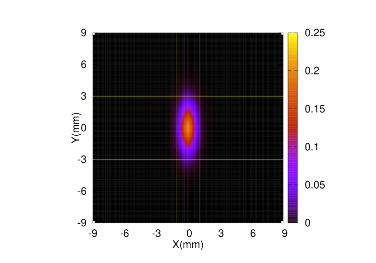
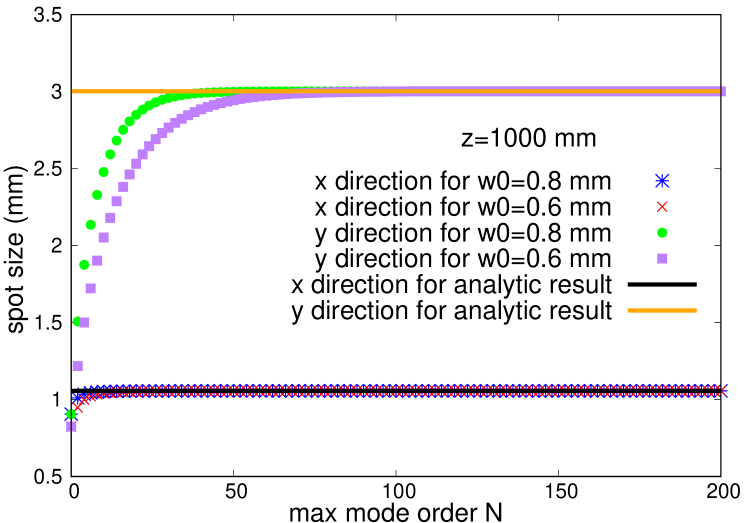
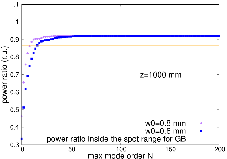
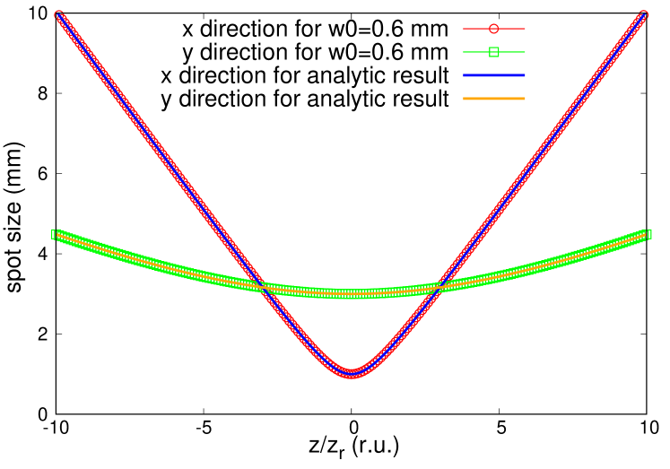
Figure 1: (a). The intensity profile for $z=$1000\text{\,}\mathrm{m}\mathrm{m}$$. (b). The estimated values of MSD spot size for different max mode order $N$ compared with the analytic spot size for $z=$1000\text{\,}\mathrm{m}\mathrm{m}$$. (c). The power ratio within the MSD spot size for different max mode order $N$ for $z=$1000\text{\,}\mathrm{m}\mathrm{m}$$. (d). The estimated values of spot size of MEM beam compared with the analytic spot size for different propagation distances.

Figure 1 shows the intensity profile for $z=$1000\text{\,}\mathrm{m}\mathrm{m}$$ of the MEM beam which represents the simple astigmatic Gaussian beam. The yellow line in Fig. 1 is the boundary of the MSD spot for the MEM beam and the green point is the estimated beam center $(0,0)$. The waist of the basic HG modes for the MEM beam is $w_{0}=$0.6\text{\,}\mathrm{m}\mathrm{m}$$ and the max mode order is $N=200$. Figures 1 and 1 show the variations for the MSD spot size and the power ratio within the MSD spot range with different max mode order $N$. The waist of the basic HG modes for the MEM beam is $w_{0}=$0.6\text{\,}\mathrm{m}\mathrm{m}$$ or $w_{0}=$0.8\text{\,}\mathrm{m}\mathrm{m}$$ and $z=$1000\text{\,}\mathrm{m}\mathrm{m}$$. The blue points in Fig. 1 shows the MSD spot size for different max mode order $N$ for $w_{0}=$0.8\text{\,}\mathrm{m}\mathrm{m}$$ in x direction, the red points show the MSD spot size for $w_{0}=$0.6\text{\,}\mathrm{m}\mathrm{m}$$ in x direction, the green points show the MSD spot size for $w_{0}=$0.8\text{\,}\mathrm{m}\mathrm{m}$$ in y direction and the purple points show the MSD spot size for $w_{0}=$0.6\text{\,}\mathrm{m}\mathrm{m}$$ in y direction. The black line and orange line in Fig. 1 show the analytic spot size for this simple astigmatic Gaussian beam in x direction and y direction respectively. The purple points in Fig. 1 show the power ratio within the MSD spot range for different max mode orders N for $w_{0}=$0.8\text{\,}\mathrm{m}\mathrm{m}$$, the blue points show the power ratio within the MSD spot range for $w_{0}=$0.6\text{\,}\mathrm{m}\mathrm{m}$$ and the orange line shows the power ratio inside the circular spot range for the Gaussian beam. When the max mode order $N$ is large enough, the MSD spot size is coincident with the analytical spot size of the input simple astigmatic Gaussian beam, no matter what the waist of the basic HG modes is. As shown in Fig. 1, the MSD spot size is coincident with the analytic spot size for the simple astigmatic Gaussian beam for different $z$. The max mode order $N$ is 200 and the waist of the basic HG modes $w_{0}$ is $0.6\text{\,}\mathrm{m}\mathrm{m}$. The red line in Fig. 1 shows the MSD spot size for different $z$ in x direction, the green line shows the MSD spot size in y direction, the blue line shows the analytical spot size in x direction and the orange line shows the analytical spot size in y direction. The MSD spot size is a hyperbolic function of $z$. The fractional beam energy concentrated inside the MSD spot range of this situation is $92.15\%$. If the max mode order $N$ is large enough, the waist $w_{0}$ of the basic HG modes will have little influence on the estimated value of MSD spot size and the power ratio within the MSD spot range.

Another non-diffracted beam concerning a shifted HG beam will be discussed in B.

3.2 Nearly-Gaussian beams

In this subsection, we will test the MSD spot size definition for some non-perfect beams as they can appear in laboratory experiments. We use the MEM to decompose these non-perfect beams and then calculate the MSD spot size and the fractional beam energy concentrated inside the MSD spot range for these beams.

3.2.1 Halo Beam

A halo beam might be produced by touching a fiber end to a monolithic fiber collimator with optical contact gel in the laboratory. If there is a small gap between the collimator and the fiber, the intensity profiles will deform like a halo as illustrated in Fig. 2:

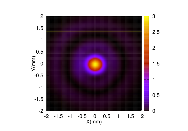
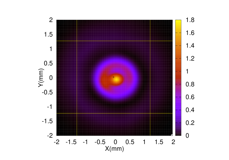
Figure 2: (a) The intensity profile for $z=$75.865\text{\,}\mathrm{m}\mathrm{m}$$ and the yellow line is the boundary of the MSD spot. (b) The intensity profile for $z=$-362.135\text{\,}\mathrm{m}\mathrm{m}$$ and the yellow line is the boundary of the MSD spot.

The ”plus” points shown in Figs. 2 and 2 mark the energy centers. The energy center in Fig. 2 is $(-0.04281,0.03558)$. It is $(-0.03492,0.02280)$ in Fig. 2. The fractional beam energy concentrated inside the spot size shown in Fig. 2 is $81.2142\%$ and $84.0180\%$ in Fig. 2. Figure 3 shows the MSD spot size for different $z$ and Fig. 3 shows the fractional beam energy concentrated inside the MSD spot for different $z$. The MSD spot size for the halo beam satisfies the hyperbolic law and the fractional beam energy concentrated inside the MSD spot size is always bigger than $80.94\%$. The waist of these HG modes is $w_{0}=$644.314\text{\,}\mu\mathrm{m}$$ and the waist plane of these HG modes are all located in the cross-section of $z=$0\text{\,}\mathrm{m}\mathrm{m}$$. The decomposition results of the MEM beam for this halo beam are shown in D.

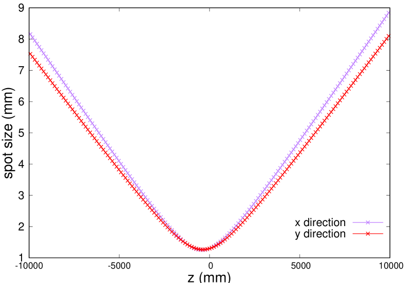
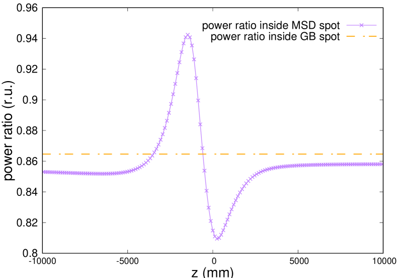
Figure 3: (a) The MSD spot size of halo beam for different $z$. (b)The fractional beam energy concentrated inside the MSD spot for different $z$.

3.2.2 Nearly-Gaussian beam II

Another non-perfect beam is shown in Fig. 4.

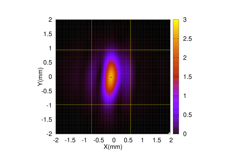
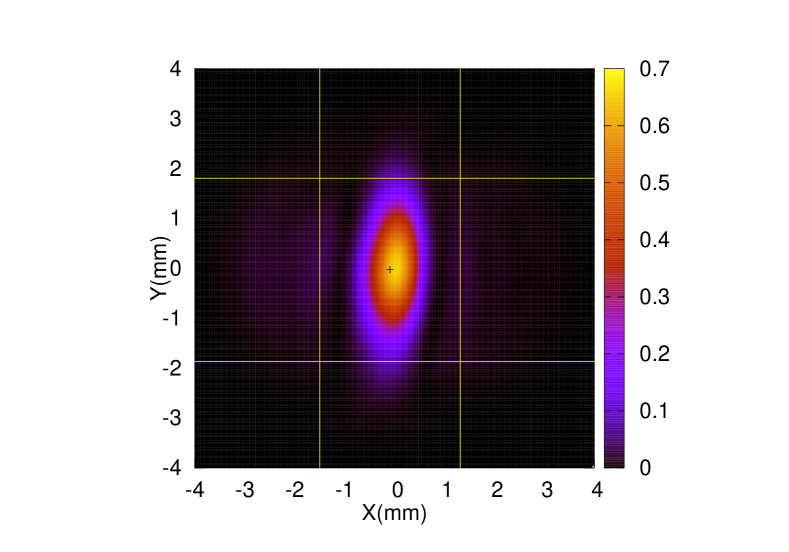
Figure 4: (a) The intensity profile for $z=$481.101\text{\,}\mathrm{m}\mathrm{m}$$ and the yellow line is the boundary of the MSD spot. (b) The intensity profile for $z=$1081.101\text{\,}\mathrm{m}\mathrm{m}$$ and the yellow line is the boundary of the MSD spot.

The ”plus” points shown in Figs. 4 and 4 mark the energy centers. The energy center in Fig. 4 is $(-0.0691484,-0.0196754)$. It is $(-0.0927757,-0.0306717)$ in Fig. 4. The fractional beam energy concentrated inside the spot size shown in Fig. 4 is $89.6420\%$ and $88.0395\%$ in Fig. 4. Figure 5 shows the MSD spot size for different $z$ and Fig. 5 shows the fractional beam energy concentrated inside the MSD spot for different $z$. The waist of these HG modes is $w_{0}=$399.465\text{\,}\mu\mathrm{m}$$ and the waist planes of these HG modes are all located in the cross-section of $z=$0\text{\,}\mathrm{m}\mathrm{m}$$. The decomposition results of the MEM beam for this beam are shown in E.

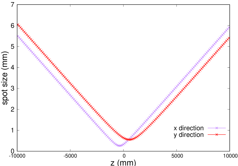
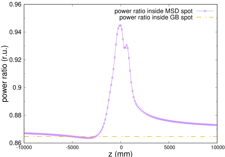
Figure 5: (a) The MSD spot size of nearly-Gaussian beam II for different $z$. (b)The fractional beam energy concentrated inside the MSD spot for different $z$.

4 MSD spot size and power ratio within the MSD spot range for top-hat beams in detection of gravitational waves in space.

In this section, we shall enter the core of our work and trace the evolution of the spot size of a top-hat beam propagating within an optical bench for a LISA or TAIJI type mission. The spot size together with the corresponding power ratio within this spot range will also be estimated. To this end, we shall first address in the following subsection the issue of hard edge diffraction of a flat top beam. The MSD spot size for a top-hat beam in a science interferometer in a LISA or TAIJI type optical bench will then be simulated. Some error analysis will then be presented to render our calculations more trustworthy.

4.1 Spot size for a top-hat beam

In this section, we investigate the performance of the MSD spot size in the top-hat beam case. Unlike the previously discussed cases, diffraction occurs at the edge of the beam and this generates divergence for the MSD spot size of a top-hat beam. The analysis will then be applied in the next subsection when we look at the propagation of a flat top beam within a distance scale dictated by the size of an optical bench in detection of gravitational waves in space.

Consider a top-hat beam which may be regarded as a plane wave truncated by a circular aperture. The complex amplitude of the top-hat beam maybe written as

$$u_{top}(x,y,0)=\left\{\begin{aligned} &\sqrt{\frac{P}{\pi}}\frac{1}{r},\ x^{2}+y^{2}\leq r^{2}\\ &0,\ x^{2}+y^{2}>r^{2},\end{aligned}\right.$$ (14)

where $r$ is the initial radius of the top-hat beam and $P$ is the total power. Here we assume the beam propagates along $+z$ direction and the wavelength of this top-hat beam is $\lambda=$1064\text{\,}\mathrm{n}\mathrm{m}$$.

As discussed in Section 2, the top-hat beam can be decomposed by MEM and the propagation of this MEM beam can be used to represent the propagation of the top-hat beam. The beam center and the propagation direction of these basic HG modes are the same as the top-hat beam in this section. The waist planes of these basic HG modes are located at the initial plane of the top-hat beam. The total power of the input top-hat beam is $P=1$ a.u.. The initial radius $r$ of the top-hat beam is $2.5\text{\,}\mathrm{m}\mathrm{m}$ here which is coincident with the top-hat beam in the paper by L. D’Arcio et al.[1]

One obvious shortcoming of the MSD spot size for the hard-edge diffraction beam is, that it is divergent [5]. The word divergent here means that the MSD spot size for the hard-edge diffraction beam is infinite (Eq. 2$\rightarrow\infty$). Rounding off the spatial intensity distribution in some reasonable way such as with a super-Gaussian edge is one choice to solve this divergence [5]. Alternatively, another choice is to truncate the limitation of the integration for MSD spot size to eliminate the large angle and evanescent waves [5]. Many criteria are proposed for the truncated limitation such as general truncated second-order moment method [6], asymptotic approximation method [7] and self-convergent beam width method [8] and many more. However, all of them introduce another free parameter which is changed by hand and can influence the final value of the MSD spot size. There is no general guidance to find a suitable value for the free parameter. These truncated methods introduce another disadvantage that they can not guarantee that the hyperbolic law and ABCD law for propagation still holds.

The MSD spot size is sensitive to the diffracted wings even if there are only few fractional parts of beam energy inside these wings [7]. Limiting the interval of integration of the MSD spot size definition to eliminate the divergence [7] can be regarded as only reserving a few dominating wings. The diffracted beam may also be decomposed by MEM as the previous section shows. The higher the HG mode order is, the more outside wings can be represented. In a sense, using a finite number of HG modes to represent the diffracted beam is similar to limiting the interval of the integration. Compared with the MSD spot size of the diffracted beam obtained by limiting the upper and lower limits of the integral, the advantages of the MSD spot of the MEM beam are that it still satisfies the ABCD law during passing through the ABCD system and still exhibits the hyperbolic function of propagation distance.

Figures 6, 6 and 6 show the intensity profiles of the MEM beams which represent the top-hat beam for the propagation distances $z=$100\text{\,}\mathrm{m}\mathrm{m}$$ , $z=$600\text{\,}\mathrm{m}\mathrm{m}$$ and $z=$3000\text{\,}\mathrm{m}\mathrm{m}$$. The waist of the basic HG modes of the MEM beam is $w_{0}=$0.5\text{\,}\mathrm{m}\mathrm{m}$$ and the max mode order $N$ of the MEM beams is $N=200$. Figures 6, 6 and 6 show the intensity distributions of the MEM beams along the x-axis of Figs. 6, 6 and 6. The vertical lines in these subfigures are the edges of the MSD spot range for different MEM beams. The blue vertical lines in these subfigures represent the MSD spot size for the MEM beam with $w_{0}=$0.25\text{\,}\mathrm{m}\mathrm{m}$$, the red lines represent $w_{0}=$0.5\text{\,}\mathrm{m}\mathrm{m}$$, the green lines represent $w_{0}=$0.75\text{\,}\mathrm{m}\mathrm{m}$$, the purple lines represent $w_{0}=$1.0\text{\,}\mathrm{m}\mathrm{m}$$ and the orange lines represent $w_{0}=$1.25\text{\,}\mathrm{m}\mathrm{m}$$. The dark-red vertical line is special and represents the spot size $w_{f}$ calculated from the paper by E. M. Drège et al.[9] A typical divergence angle $\theta_{f}$ is defined as the distance between the central brightest point and the point where the intensity is $\frac{1}{e^{2}}$ of the maximum intensity value over the large propagation distance $z$. Furthermore, the spot size $w_{f}$ is defined as the divergence angle $\theta_{f}$ times the propagation distance $z$. This means the spot size $w_{f}$ represents the distance between the central brightest point and the point where the intensity is $\frac{1}{e^{2}}$ of the maximum intensity value in the far-field. In the far-field, this spot size $w_{f}$ and the far-field divergence $\theta_{f}$ angle is a function of wavelength $\lambda$ and the radius of the circular aperture $R$ [9]

$$\theta_{f}=\frac{2.5838\lambda}{2\pi R},$$ (15a)

$$w_{f}=\theta_{f}\cdot z.$$ (15b)

The max mode orders $N$ in the above cases are fixed to be 200. As a matter of fact, the max mode order $N$ may also influence the MSD spot size of a top-hat beam. Figures 7, 7 and 7 show the variation of the spot size with the max mode order $N$ for the propagation distances $z=$100\text{\,}\mathrm{m}\mathrm{m}$$, $z=$600\text{\,}\mathrm{m}\mathrm{m}$$ and $z=$3000\text{\,}\mathrm{m}\mathrm{m}$$. The variation of the corresponding power ratio within the MSD spot range are shown in Figs. 7, 7 and 7 for the propagation distances $z=$100\text{\,}\mathrm{m}\mathrm{m}$$ , $z=$600\text{\,}\mathrm{m}\mathrm{m}$$ and $z=$3000\text{\,}\mathrm{m}\mathrm{m}$$.

As mentioned before, the MSD spot size is infinite in hard-edge diffraction situations such as the top-hat beam here. Using the MEM, we can get a finite MSD spot size for the diffracted beam. However, this finite MSD spot size is dependent on the max mode order $N$ and the waist $w_{0}$ of the basic HG modes. For any fixed propagation distance $z$, the MSD spot size diverges with the increasing mode order $N$. As Fig. 6 shows, all these spot ranges are large enough to contain the main part of the intensity patterns except for $w_{f}$. The spot size calculated from the analytical divergence angle of the top-hat beam $w_{f}$ is so small that we can not use it here.

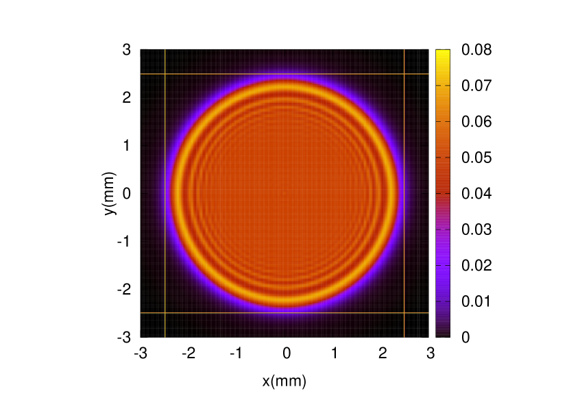
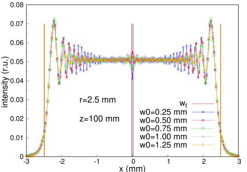
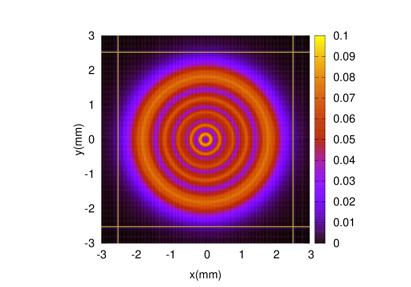
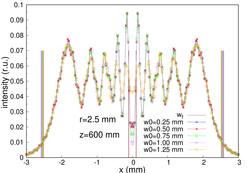
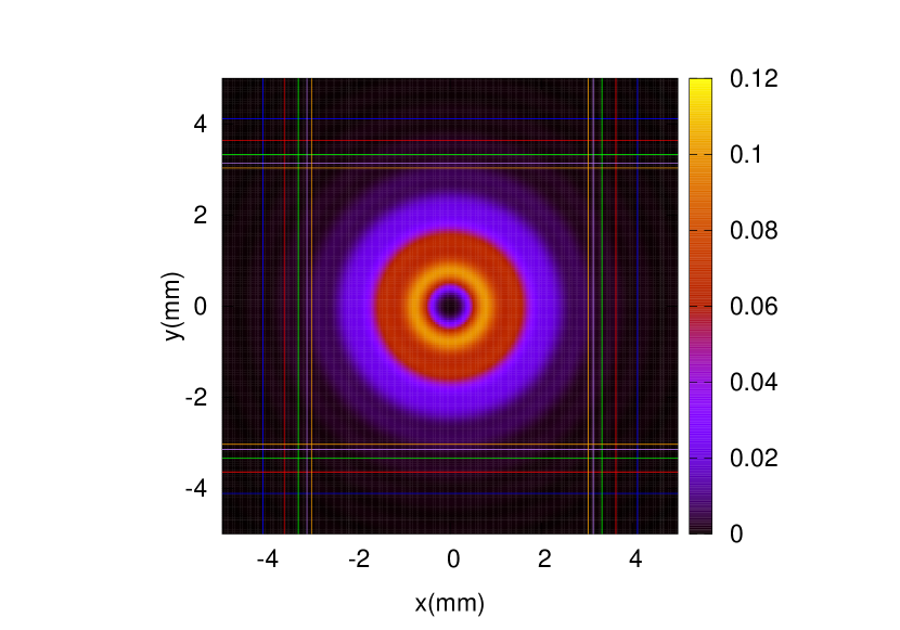
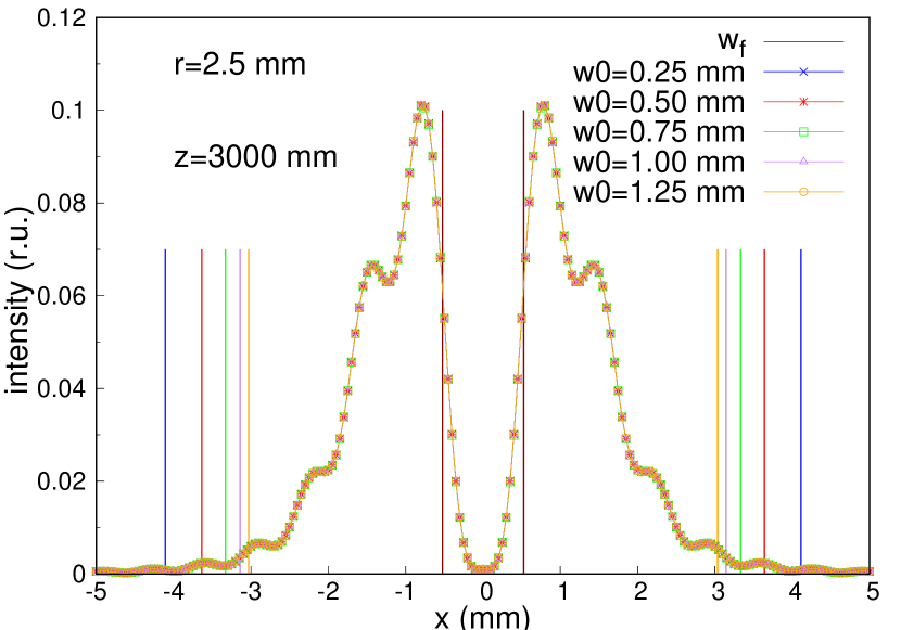
Figure 6: The intensity profiles of the simulated top-hat beam for the propagation distance $z=$100\text{\,}\mathrm{m}\mathrm{m}$$ (a), $z=$600\text{\,}\mathrm{m}\mathrm{m}$$ (c) or $z=$3000\text{\,}\mathrm{m}\mathrm{m}$$ (e). The intensity distributions of the simulated top-hat beam along x-axis for the propagation distance $z=$100\text{\,}\mathrm{m}\mathrm{m}$$ (b), $z=$600\text{\,}\mathrm{m}\mathrm{m}$$ (d) or $z=$3000\text{\,}\mathrm{m}\mathrm{m}$$ (f).

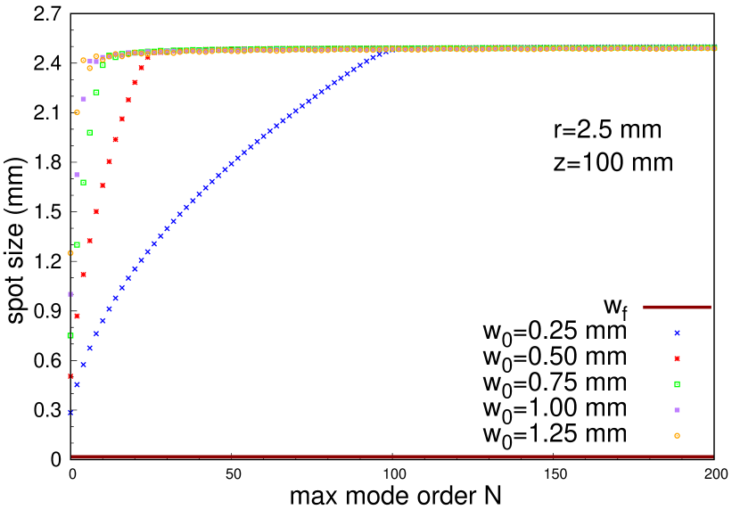
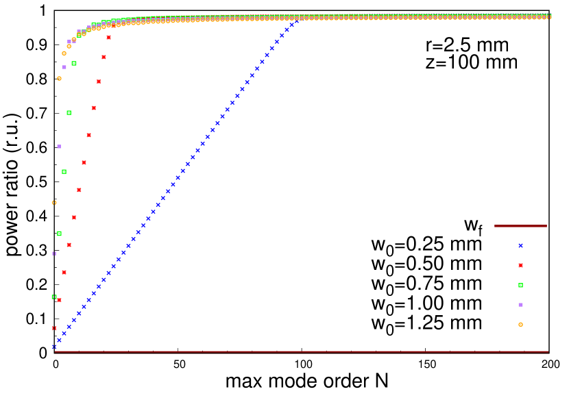
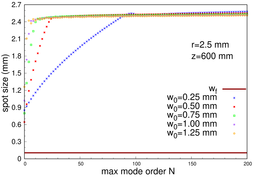
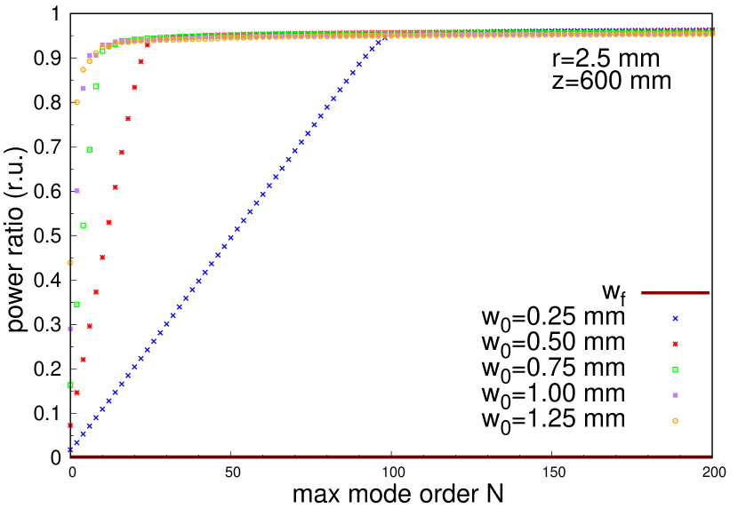
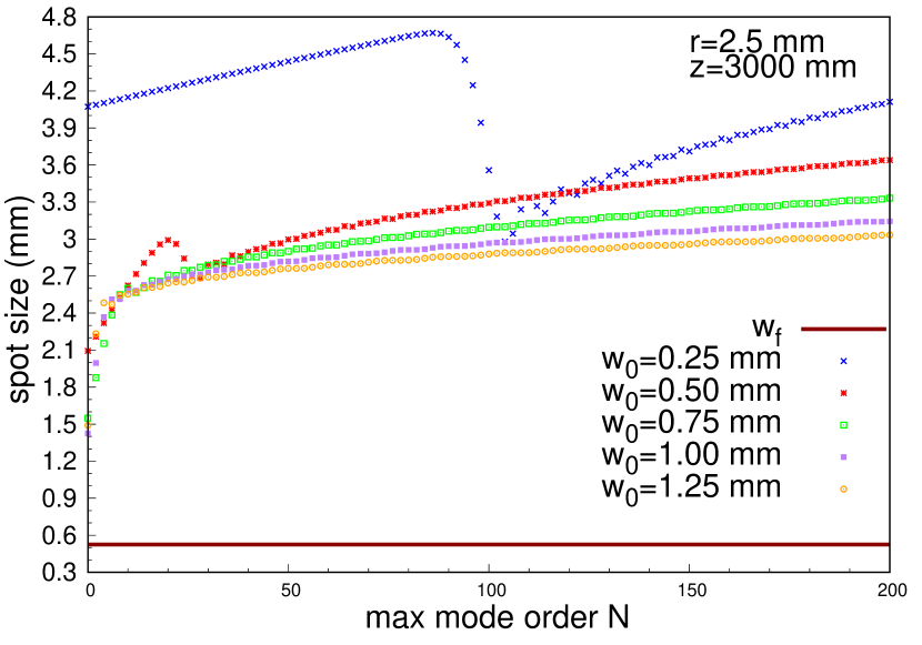
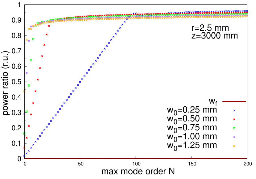
Figure 7: The MSD spot size of the simulated top-hat beam for different max mode order $N$ with the propagation distance $z=$100\text{\,}\mathrm{m}\mathrm{m}$$ (a), $z=$600\text{\,}\mathrm{m}\mathrm{m}$$ (c) or $z=$3000\text{\,}\mathrm{m}\mathrm{m}$$ (e). The power ratio within the MSD spot range of the simulated top-hat beam for different max mode order $N$ with the propagation distance $z=$100\text{\,}\mathrm{m}\mathrm{m}$$ (b), $z=$600\text{\,}\mathrm{m}\mathrm{m}$$ (d) or $z=$3000\text{\,}\mathrm{m}\mathrm{m}$$ (f).

The Fresnel number for this top-hat beam is

$$F(z)=\frac{r^{2}}{z\lambda}.$$ (16)

The Fresnel numbers for propagation distances $z=$100\text{\,}\mathrm{m}\mathrm{m}$$, $z=$600\text{\,}\mathrm{m}\mathrm{m}$$ and $z=$3000\text{\,}\mathrm{m}\mathrm{m}$$ are $F(100)=58.7406$, $F(600)=9.7901$, $F(3000)=1.9580$. All of these three cross-sections are located in the near field of this top-hat beam because the Fresnel numbers are bigger than $1$. When the max mode order $N$ is large enough, the estimated spot ranges for these MEM beams are almost the same for very near fields such as $z=$100\text{\,}\mathrm{m}\mathrm{m}$$ and $z=$600\text{\,}\mathrm{m}\mathrm{m}$$. As for the not very near field such as $z=$3000\text{\,}\mathrm{m}\mathrm{m}$$, the estimated spot ranges for different MEM beams are obviously different. The differences of the power ratio within the corresponding MSD spot range are small for $z=$100\text{\,}\mathrm{m}\mathrm{m}$$, $z=$600\text{\,}\mathrm{m}\mathrm{m}$$ and $z=$3000\text{\,}\mathrm{m}\mathrm{m}$$. The larger the waist for the basic HG modes is, the smaller the MSD spot size and power ratio within the MSD spot range are. Diffracted aberration Gaussian beam as another diffracted beam case will be discussed in C.

4.2 Spot size estimation for a top-hat beam in Science Interferometer

In this subsection, we are in a position to numerically track the evolution of the spot size of a flat top beam for the science interferometer in an optical bench for a LISA or TAIJI type mission. Further we will also argue that, despite of the divergence behaviour of the MSD spot size for a flat top beam, our analysis still draws a reliable conclusion.

Consider one of the optical designs for the LISA optical bench [1] and we take a top-hat beam of a science interferometer as a representative example of optical beam propagation within the optical bench for our investigation. In Fig. 8, the science interferometer subsystem of this optical bench is shown. The initial radius of the input top-hat beam in the exit pupil plane is $2.5\text{\,}\mathrm{m}\mathrm{m}$ [1]. Given that the optical bench design of neither of both missions is available yet, we can only estimate that the propagation distances in the science interferometer on the optical bench will be in the order of tens of centimeters. Consequently, we test here the spot size evolution for propagation distances up to $60\text{\,}\mathrm{c}\mathrm{m}$. We use Eqs. 11 and 12 to calculate the MSD spot size and the corresponding power ratio within the spot range here.

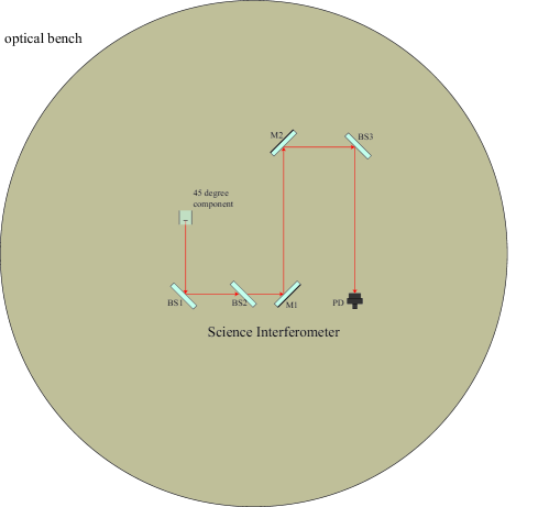
Figure 8: Science interferometer qualitatively derived from paper[1], shown only starting from the $45$ degree component delivering the received beam from the telescope onto the optical bench, neglecting imaging systems and redundancy.

Figures 9, 9 and 9 show the MSD spot sizes for different propagation distances $z$ of different MEM beams which represent the top-hat beam with initial radii $r=$2\text{\,}\mathrm{m}\mathrm{m}$$, $2.5\text{\,}\mathrm{m}\mathrm{m}$ or $3\text{\,}\mathrm{m}\mathrm{m}$ respectively. The settings of these MEM beams are the same except for the waist size $w_{0}$ of basic HG modes in the same subfigure. The max mode order $N$ of these MEM beams is equal to $200$. The origin and direction of the basic HG modes of MEM beams are the same as the origin and direction of the input top-hat beam.

Figures 9, 9 and 9 show the power ratio within the MSD spot range for different propagation distances $z$ of different MEM beams which represent the top-hat beam with initial radii $r=$2\text{\,}\mathrm{m}\mathrm{m}$$, $2.5\text{\,}\mathrm{m}\mathrm{m}$ or $3\text{\,}\mathrm{m}\mathrm{m}$ respectively. The settings of these MEM beams are the same as the settings in Figs. 9, 9 and 9.

For certain MEM beams, the MSD spot size increases with the propagation distance and it’s the hyperbolic function of propagation distance $z$ [17]. For certain propagation distances $z$, the MSD spot size increases as the waist size $w_{0}$ of the basic HG modes of the MEM beam decreases. As we discussed before, even though the MSD spot size of the MEM beam representing diffracted beams is finite, it is not unique for the corresponding diffracted beam. The MSD spot size growth rate increases with propagation distance. Furthermore, this growth rate increases as the waist size $w_{0}$ of basic HG beams decreases or the initial radius $r$ of the top-hat beam decreases.

For certain MEM beams, the power ratio within the MSD spot range decreases as the propagation distance $z$ increases here. For certain propagation distances $z$, the power ratio within the MSD spot range decreases as the waist size $w_{0}$ of basic HG modes increases. The growth rate of the power ratio within the MSD spot range increases with decreasing initial radii $r$ of the top-hat beam.

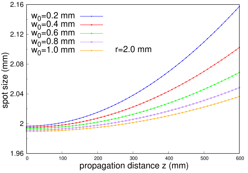
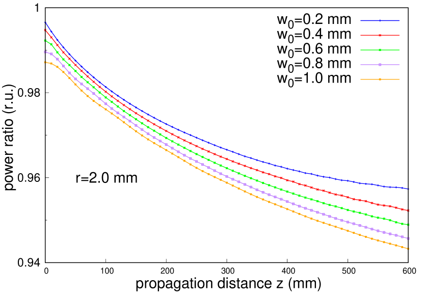
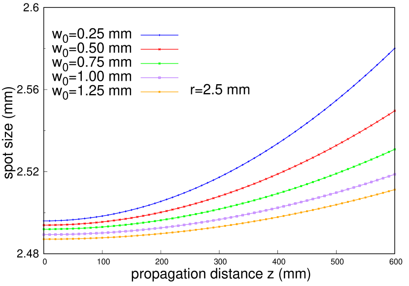
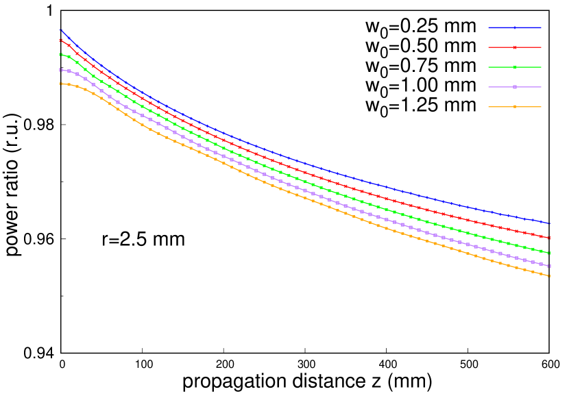
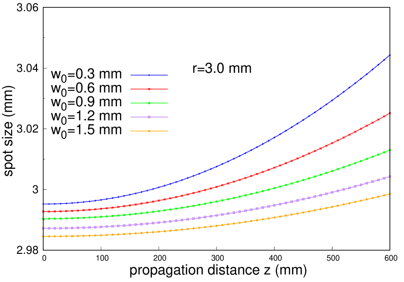
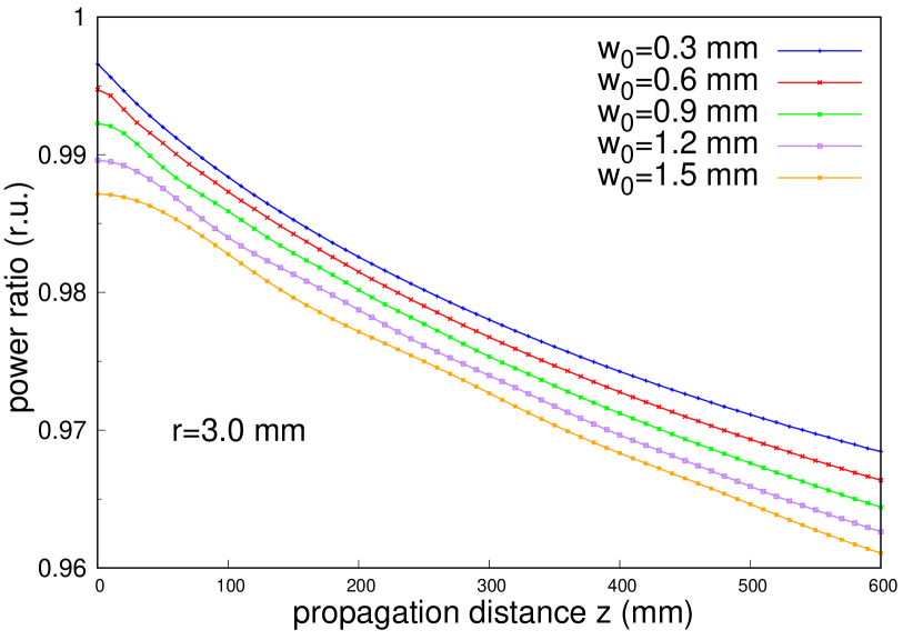
Figure 9: The MSD spot sizes for different propagation distance $z$ for the top-hat beams with initial radii $r=$2.0\text{\,}\mathrm{m}\mathrm{m}$$ (a),$r=$2.5\text{\,}\mathrm{m}\mathrm{m}$$ (c) or $r=$3.0\text{\,}\mathrm{m}\mathrm{m}$$ (e). The power ratio within the MSD spot range for different propagation distance $z$ of the top-hat beams with different initial radii $r=$2.0\text{\,}\mathrm{m}\mathrm{m}$$ (b),$r=$2.5\text{\,}\mathrm{m}\mathrm{m}$$ (d) or $r=$3.0\text{\,}\mathrm{m}\mathrm{m}$$ (f).

4.3 Error analysis

In the previous section, we qualitatively discussed the performance of MSD spots for a science interferometer. In this part, we use error analysis to quantitatively discuss the performance of MSD spot size. The estimated errors of the MSD spot size and the estimated errors of the power ratio within the MSD spot range are small enough to be negligible for the top-hat beam initial radius from $2$-3\text{\,}\mathrm{m}\mathrm{m}$$ in the propagation distance range $z\in[0,600]$ $\text{\,}\mathrm{m}\mathrm{m}$. The power ratios within the MSD spot ranges are large enough for the top-hat beam initial radius from $2$-3\text{\,}\mathrm{m}\mathrm{m}$$ in the propagation distance range $z\in[0,600]$ $\text{\,}\mathrm{m}\mathrm{m}$. This means that the estimated values of MSD spot size work well in a science interferometer in the detection of gravitational waves in space.

Unphysical decomposition parameters such as the waist $w_{0}$ of basic HG modes can influence the value of the MSD spot size of an MEM beam. It is necessary to estimate the effect of the unphysical decomposition parameter $w_{0}$ on the MSD spot size of a top-hat beam in a science interferometer. Here we define the estimated error of the MSD spot size of the top-hat beam as twice the ratio of the difference between the maximum value of the MSD spot size for a certain propagation distance and the minimum value of the MSD spot size for the same propagation distance to the sum of this maximum value and minimum value

$$err_{spot}(z)=2\frac{w_{max}(z)-w_{min}(z)}{w_{max}(z)+w_{min}(z)},$$ (17)

where $w_{max}(z)$ is the maximum value of the MSD spot size for propagation distance $z$ and $w_{min}(z)$ is the minimum value of the MSD spot size for propagation distance $z$.

Similar to the estimated error definition of the MSD spot, we define the estimated error of the power ratio within the MSD spot range as

$$err_{p_{r}}(z)=2\frac{p_{r_{max}}(z)-p_{r_{min}}(z)}{p_{r_{max}}(z)+p_{r_{min}}(z)},$$ (18)

where $p_{r_{max}}(z)$ is the maximum value of the power ratio within the MSD spot range for propagation distance $z$ and $p_{r_{min}}(z)$ is the minimum value of the power ratio within the MSD spot range for propagation distance $z$.

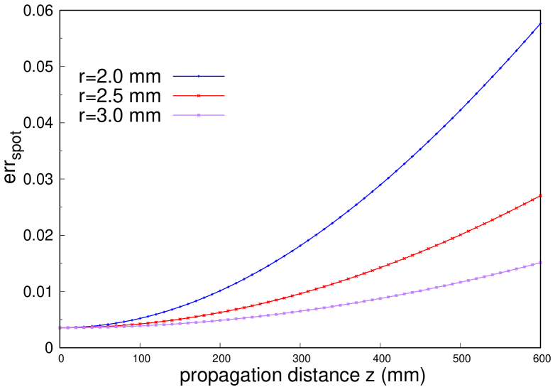
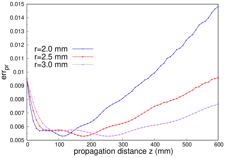
Figure 10: (a) The estimated error of MSD spot sizes for different propagation distance $z$. (b) The estimated error of the power ratio within the MSD spot range for different propagation distance $z$.

Figure 10 shows the estimated error of the MSD spot size for different propagation distances $z$ of different MEM beams which represent the top-hat beam with the initial radii $r=$2\text{\,}\mathrm{m}\mathrm{m}$$, $2.5\text{\,}\mathrm{m}\mathrm{m}$ and $3\text{\,}\mathrm{m}\mathrm{m}$. It is obvious that the estimated error of MSD spot size for the top-hat beam increases with the propagation distance $z$. The maximum estimated error of MSD spot size in these simulations of the top-hat beam with $2\text{\,}\mathrm{m}\mathrm{m}$ initial radius is $5.764\%$ for $z=$60\text{\,}\mathrm{c}\mathrm{m}$$ and the max value of MSD spot size in Fig. 9 is $2.157\text{\,}\mathrm{m}\mathrm{m}$ for $z=$60\text{\,}\mathrm{c}\mathrm{m}$$. For the top-hat beam with $2.5\text{\,}\mathrm{m}\mathrm{m}$ initial radius, the maximum estimated error of MSD spot size is $2.705\%$ for $z=$60\text{\,}\mathrm{c}\mathrm{m}$$ and the max value of MSD spot size in Fig. 9 is $2.58\text{\,}\mathrm{m}\mathrm{m}$ for $z=$60\text{\,}\mathrm{c}\mathrm{m}$$. As for the top-hat beam with $3\text{\,}\mathrm{m}\mathrm{m}$ initial radius, the maximum estimated error of MSD spot size is $1.514\%$ for $z=$60\text{\,}\mathrm{c}\mathrm{m}$$ and the max value of MSD spot size in Fig. 9 is $3.044\text{\,}\mathrm{m}\mathrm{m}$ for $z=$60\text{\,}\mathrm{c}\mathrm{m}$$. The max estimated error of the MSD spot size decreases when the initial radius of the top-hat beam increases. For the science interferometer that we investigated here, the initial radius $r$ of the input top-hat beam is $2.5\text{\,}\mathrm{m}\mathrm{m}$, and the corresponding maximum estimated error of MSD spot size is $2.705\%$ for $z=$60\text{\,}\mathrm{c}\mathrm{m}$$. The estimated error of the MSD spot size for this situation is so small that we can use this MSD spot size to represent the spot size of the top-hat beam here. If the initial radius r is changed to $2\text{\,}\mathrm{m}\mathrm{m}$ or $3\text{\,}\mathrm{m}\mathrm{m}$, the estimated error of the MSD spot size would still be small enough to use.

Figure 10 shows the estimated errors of the power ratio within the MSD spot range for different propagation distances $z$ of different MEM beams which represent the top-hat beams with the initial radii $r=$2\text{\,}\mathrm{m}\mathrm{m}$$, $2.5\text{\,}\mathrm{m}\mathrm{m}$ and $3\text{\,}\mathrm{m}\mathrm{m}$. The maximum estimated error of the power ratio within the MSD spot range of the top-hat beam with $2\text{\,}\mathrm{m}\mathrm{m}$ initial radius is $1.481\%$ for $z=$60\text{\,}\mathrm{c}\mathrm{m}$$. For the top-hat beam with $2.5\text{\,}\mathrm{m}\mathrm{m}$ initial radius, the maximum estimated error of the power ratio within the MSD spot range of the top-hat beam is $0.959\%$ for $z=$60\text{\,}\mathrm{c}\mathrm{m}$$. As for the top-hat beam with $3\text{\,}\mathrm{m}\mathrm{m}$ initial radius, the maximum estimated error of MSD spot size is $0.951\%$ for $z=$0\text{\,}\mathrm{c}\mathrm{m}$$. The fractional part of the beam energy concentrated inside the MSD spot range is always larger than $94.326\%$ for the top-hat beam with $2\text{\,}\mathrm{m}\mathrm{m}$ initial radius in Fig. 9, $95.351\%$ for the top-hat beam with $2.5\text{\,}\mathrm{m}\mathrm{m}$ initial radius in Fig. 9 and $95.66\%$ for the top-hat beam with $3\text{\,}\mathrm{m}\mathrm{m}$ initial radius in Fig. 9. The maximum estimated error of the power ratio within the MSD spot range for the top-hat beam with $2.5\text{\,}\mathrm{m}\mathrm{m}$ initial radius is the smallest in these three cases. If the initial radius $r$ is changed from $2.5\text{\,}\mathrm{m}\mathrm{m}$ to $2\text{\,}\mathrm{m}\mathrm{m}$ or $3\text{\,}\mathrm{m}\mathrm{m}$, the estimated error of the MSD spot size would still be small enough to use.

There are two reasons why the power inside the MSD spot range does not equal the power of the input top-hat beam. First of all, the power loss appears in the MEM process because of the finite decomposition mode order. This power loss is independent of the propagation distance $z$ and it increases with the waist size $w_{0}$ of basic HG modes. Secondly, a top-hat beam is a diffracted beam, parts of the diffracted wings always appear outside a finite range. This power loss is dependent on the propagation distance $z$. At the same time, we notice that the MSD spot size increases with the propagation distance $z$. As mentioned before, the power ratio within the MSD spot range decreases as the propagation distance $z$ increases. This means that the rate of increase of the MSD spot size is slightly slower than the diffusion rate of the diffracted wings.

In the above discussion, we find that the estimated errors of the MSD spot size, as well as the estimated errors of the power ratio within the MSD spot range, are small and the power ratios within the MSD spot range are large enough for the top-hat beam initial radius from $2$-3\text{\,}\mathrm{m}\mathrm{m}$$ in the propagation distance range $z\in[0,600]$ $\text{\,}\mathrm{m}\mathrm{m}$.

The optical elements on the LISA Pathfinder optical bench had a size of $15\times 20\times 7$\text{\,}\mathrm{m}\mathrm{m}$$ [22]. The largest spot size for the top-hat beam in a science interferometer here is $2.580\text{\,}\mathrm{m}\mathrm{m}$. The usual practice of the optical element’s half width is designed to be approximately equal or slightly larger than three times the spot sizes of the input beams to avoid the clipping problem [5]. Using this rule, the size of the optical elements can be $15.48\text{\,}\mathrm{m}\mathrm{m}$. Based on this size and the size of the optical elements for LISA Pathfinder, we suggest that also space-based gravitational wave detectors like LISA and TAIJI will use comparable component sizes.

Depending on the optical designs, i.e. particularly the aperture sizes and potential use of imaging optics, the given equations in Section 2 can be used to derive the optimal size of all mirrors and beam splitters. This optimal size means that the components are small and lightweight but at the same time, large enough to prevent beam clipping. The present work will serve as a useful guide in the future system design of the optical bench and the sizes of the optical components.

5 Conclusion

In this paper, a slightly different variant of the definition of spot size is proposed, with which we calculate the MSD spot size of a light beam for arbitrary propagation distances. Even with diffraction taken into account, the definition still upholds the hyperbolic law and ABCD law of the MSD spot size. Though the MSD spot size for a diffracted MEM beam is dependent on the decomposition parameters such as the max mode order and the waist of the basic HG modes, it is shown that, for different reasonable choices of parameters, the estimated error for the MSD spot size and the power ratio within the MSD spot range will have little effect on our drawn conclusion. With the help of this method, optical systems such as the interferometers in space based gravitational wave detectors can be efficiently tested for beam clipping.

Our study results provide a method to allow for an optimal design of optical systems with top-hat or other types of non-Gaussian beams. Furthermore, it allows testing the interferometry of space-based gravitational wave detectors for beam clipping in optical simulations. The present work will serve as a useful guide in the future system design of the optical bench and the sizes of the optical components.

6 Acknowledgements

We thank Prof. Yun-Kau Lau and Apl. Prof. Gerhard Heinzel for the useful discussions. This work has been supported in part by the National Key Research and Development Program of China under Grant No.2020YFC2201501, the National Science Foundation of China (NSFC) under Grants No. 12147103 (special fund to the center for quanta-to-cosmos theoretical physics), No. 11821505, the Strategic Priority Research Program of the Chinese Academy of Sciences under Grant No. XDB23030100, and the Chinese Academy of Sciences (CAS) and the Max Planck Society (MPG) in the framework of the LEGACY cooperation on low-frequency gravitational wave astronomy (M.IF.A.QOP18098). Likewise, we gratefully acknowledge the German Space Agency, DLR and support by the Federal Ministry for Economic Affairs and Energy based on a resolution of the German Bundestag (FKZ50OQ1801) as well as the Deutsche Forschungsgemeinschaft (DFG) funding the Cluster QuantumFrontiers (EXC2123, Project ID 390837967) for funding the work contributions by Gudrun Wanner. We gratefully acknowledge DFG for funding the Collaborative Research Centres CRC 1464: TerraQ – Relativistic and Quantum-based Geodesy and the Clusters of Excellence PhoenixD (EXC 2122, Project ID 390833453). In this paper, the part of the numerical computation is finished by TAIJI Cluster.

Appendix A power ratio within the MSD spot range

Here, we deduce the relationship between the power ratio within the MSD spot range and $z$. The intensity of the MEM beam can be represented as

$$\begin{split}I=&\sum\limits_{m_{1}=0}^{N}\sum\limits_{n_{1}=0}^{N-m_{1}}|a_{m_{1}n_{1}}|^{2}|u_{m_{1}n_{1}}(x,y,z)|^{2}+2\sum\limits_{m_{1}=0}^{N}\sum\limits_{n_{1}=0}^{N-m_{1}}\sum\limits_{m_{2}=0}^{N}\sum\limits_{n_{2}=0}^{N-m_{2}}|a_{m_{1}n_{1}}||a_{m_{2}n_{2}}|\\ &\cdot|u_{m_{1}n_{1}}(x,y,z)||u_{m_{2}n_{2}}(x,y,z)|\\ &\cdot\cos{(\beta_{m_{1}n_{1}}+\phi_{m_{1}n_{1}}-\beta_{m_{2}n_{2}}-\phi_{m_{2}n_{2}})}\quad|\text{for}\ (m_{2}\neq m_{1}\ \text{or}\ n_{2}\neq n_{1}),\end{split}$$ (19)

where $(m_{1},n_{1})$, $(m_{2},n_{2})$ are two of the basic HG modes of the MEM beam and $N$ is the max mode order of the MEM beam. The integrand of Eq. 12 is

$$\begin{split}\frac{I}{P_{MEM}}=&\frac{1}{\sum\limits_{m_{1}=0}^{N}\sum\limits_{n_{1}=0}^{N-m_{1}}|a_{m_{1}n_{1}}|^{2}}\frac{1}{w(z)^{2}}\exp{\left(-2\frac{x^{2}+y^{2}}{w(z)^{2}}\right)}\\ &\cdot\left(\sum\limits_{m_{1}=0}^{N}\sum\limits_{n_{1}=0}^{N-m_{1}}|a_{m_{1}n_{1}}|^{2}c_{m_{1}n_{1}}^{2}H_{m_{1}}^{2}\left(\frac{\sqrt{(}2)x}{w(z)}\right)H_{n_{1}}^{2}\left(\frac{\sqrt{(}2)y}{w(z)}\right)\right.\\ &+2\sum\limits_{m_{1}=0}^{N}\sum\limits_{n_{1}=0}^{N-m_{1}}\sum\limits_{m_{2}=0}^{N}\sum\limits_{n_{2}=0}^{N-m_{2}}|a_{m_{1}n_{1}}||a_{m_{2}n_{2}}|c_{m_{1}n_{1}}c_{m_{2}n_{2}}\\ &\cdot H_{m_{1}}\left(\frac{\sqrt{(}2)x}{w(z)}\right)H_{n_{1}}\left(\frac{\sqrt{(}2)y}{w(z)}\right)H_{m_{2}}\left(\frac{\sqrt{(}2)x}{w(z)}\right)H_{n_{2}}\left(\frac{\sqrt{(}2)y}{w(z)}\right)\\ &\left.\cdot\cos{\left(\beta_{m_{1}n_{1}}-\beta_{m_{2}n_{2}}+\left(m_{1}+n_{1}-m_{2}-n_{2}\right)\zeta(z)\right)}\right).\end{split}$$ (20)

Rewrite Eqs. 10a, 10b, 11c and 11f as

$$s_{x}(z)=f_{1}(z)w(z),$$ (21a)

$$s_{y}(z)=f_{2}(z)w(z),$$ (21b)

$$w_{x}(z)=f_{3}(z)w(z),$$ (21c)

$$w_{y}(z)=f_{4}(z)w(z).$$ (21d)

$f_{1}(z)$, $f_{2}(z)$, $f_{3}(z)$ and $f_{4}(z)$ are dependent on $z$ because of the Gouy phase part. Set $u=\frac{\sqrt{2}x}{w(z)}$ and $v=\frac{\sqrt{2}y}{w(z)}$, then

$$\begin{split}\frac{I}{P_{MEM}}=&\frac{I}{P_{MEM}}(u,v,z)=\frac{1}{\sum\limits_{m_{1}=0}^{N}\sum\limits_{n_{1}=0}^{N-m_{1}}|a_{m_{1}n_{1}}|^{2}}\frac{1}{w(z)^{2}}\exp{\left(-u^{2}-v^{2}\right)}\\ &\cdot\left(\sum\limits_{m_{1}=0}^{N}\sum\limits_{n_{1}=0}^{N-m_{1}}|a_{m_{1}n_{1}}|^{2}c_{m_{1}n_{1}}^{2}H_{m_{1}}^{2}\left(u\right)H_{n_{1}}^{2}\left(v\right)\right.\\ &+2\sum\limits_{m_{1}=0}^{N}\sum\limits_{n_{1}=0}^{N-m_{1}}\sum\limits_{m_{2}=0}^{N}\sum\limits_{n_{2}=0}^{N-m_{2}}|a_{m_{1}n_{1}}||a_{m_{2}n_{2}}|c_{m_{1}n_{1}}c_{m_{2}n_{2}}\\ &\cdot H_{m_{1}}\left(u\right)H_{n_{1}}\left(v\right)H_{m_{2}}\left(u\right)H_{n_{2}}\left(v\right)\\ &\left.\cdot\cos{\left(\beta_{m_{1}n_{1}}-\beta_{m_{2}n_{2}}+\left(m_{1}+n_{1}-m_{2}-n_{2}\right)\zeta(z)\right)}\right).\end{split}$$ (22)

$$\int_{s_{x}(z)-w_{x}(z)}^{s_{x}(z)+w_{x}(z)}dx=\int_{\sqrt{2}(f_{1}(z)-f_{3}(z))}^{\sqrt{2}(f_{1}(z)+f_{3}(z))}\frac{w(z)}{\sqrt{2}}du,$$ (23a)

$$\int_{s_{y}(z)-w_{y}(z)}^{s_{y}(z)+w_{y}(z)}dy=\int_{\sqrt{2}(f_{2}(z)-f_{4}(z))}^{\sqrt{2}(f_{2}(z)+f_{4}(z))}\frac{w(z)}{\sqrt{2}}dv$$ (23b)

Using Eq. 22 and Eq. 23 in the definition of the power ratio within the MSD spot range Eq. 12, we find $\epsilon_{P_{spot}}$ is obviously dependent on $z$

$$\epsilon_{P_{spot}}=\int_{\sqrt{2}(f_{1}(z)-f_{3}(z))}^{\sqrt{2}(f_{1}(z)+f_{3}(z))}\int_{\sqrt{2}(f_{2}(z)-f_{4}(z))}^{\sqrt{2}(f_{2}(z)+f_{4}(z))}\frac{w(z)^{2}}{2}\frac{I}{P_{MEM}}(u,v,z)dudv.$$ (24)

The integrand $\frac{w(z)^{2}}{2}\frac{I}{P_{MEM}}(u,v,z)$ is still dependent on $z$ because of the Gouy phase part. According to the property of the $Arctan$ function, the Gouy phase always can be regarded as a constant when $z$ is large enough. If $z$ is large enough, $f_{1}(z)$, $f_{2}(z)$, $f_{3}(z)$ and $f_{4}(z)$, the integrand $\frac{w(z)^{2}}{2}\frac{I}{P_{MEM}}(u,v,z)$ and $\epsilon_{P_{spot}}$ will be independent from $z$.

Appendix B shifted HG beam

Sometimes, it’s not easy to find the center of the beam in the experiment. The paper by X. Xue et al. [23] shows that people can use the intensity profiles to find the superposition of a finite number of HG modes which can represent the experimental beam. The centers of these HG modes are usually not the same as the center of the input experimental beam. If the center of these decomposed HG modes is set to the same as the origin of the experiment of the beam, we would do a more accurate component analysis. Here, we would like to test Eqs. 10a, 10b, 11c and 11f, especially the estimated value of beam center in the shifted HG Gaussian beam situation. The shifted beam means that the center of the beam is not the same as the centers of decomposed HG modes. For instance, we set the order of this shifted HG beam as $(1,0)$, and its origin is not located at the brightest point. Assume the waist of this shifted HG beam is $w_{0}=$1\text{\,}\mathrm{m}\mathrm{m}$$, the propagation direction is $(0,0,1)$ and the center is $(1,0)$. The electric field of this input shifted HG beam is

$$\begin{split}E_{in}=u_{in}\exp{\left(i\omega t\right)}=&\sqrt{\frac{P}{\pi}}\frac{1}{w(z)}H_{1}\left(\frac{\sqrt{2}(x-1)}{w(z)}\right)H_{0}\left(\frac{\sqrt{2}y}{w(z)}\right)\exp{\left(-\frac{(x-1)^{2}+y^{2}}{w^{2}(z)}\right)}\\ &\times\exp{\left(-ikz-ik\frac{(x-1)^{2}+y^{2}}{2R(z)}+i2\zeta(z)+i\omega t\right)}.\end{split}$$ (25)

These symbols are defined in Section 2. Here we use two different waists $0.4\text{\,}\mathrm{m}\mathrm{m}$ and $0.5\text{\,}\mathrm{m}\mathrm{m}$ for the finite number of HG modes. The direction of these HG modes is the same as the input beam. The centers of these HG modes are $(0,0)$. The decomposition happens in the waist plane of the shifted HG beam.

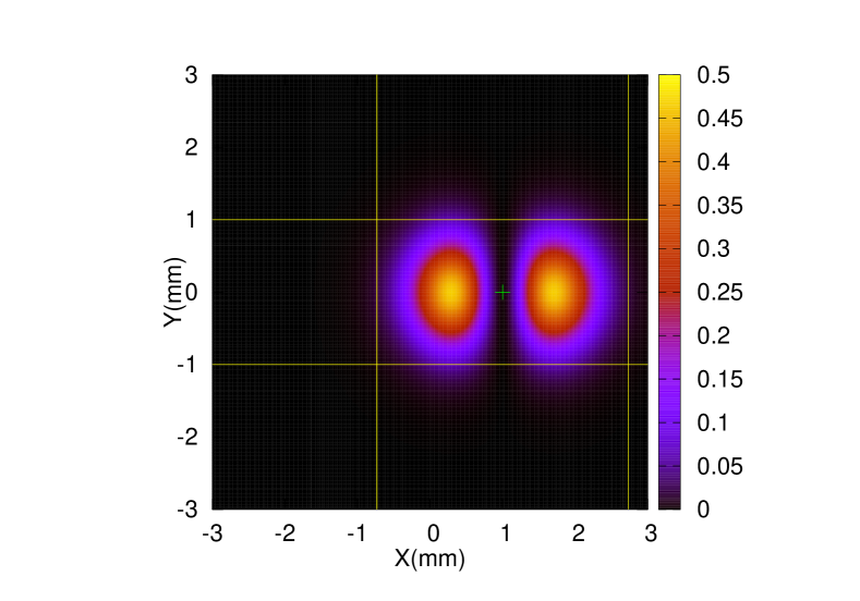
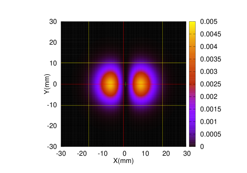
Figure 11: (a). The intensity profile for $z=$100\text{\,}\mathrm{m}\mathrm{m}$$. (b) .The intensity profile for $z=$30\,000\text{\,}\mathrm{m}\mathrm{m}$$.

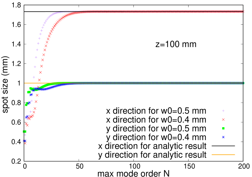
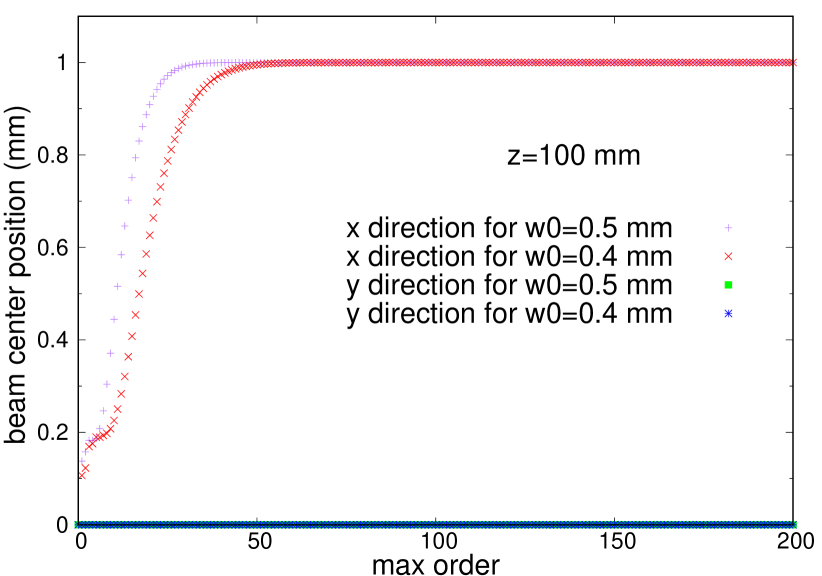
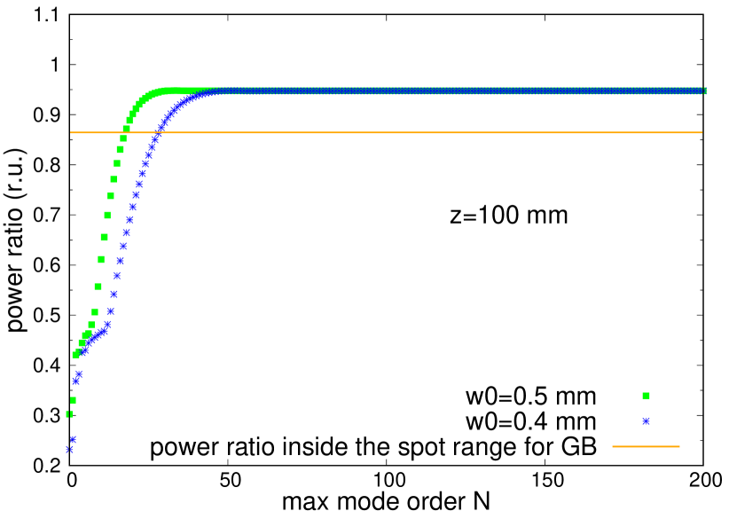
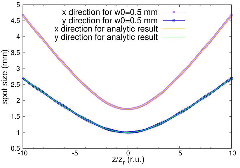
Figure 12: (a) The estimated values of spot size for different max decomposed mode order superpositions of $z=$100\text{\,}\mathrm{m}\mathrm{m}$$. (b) The estimated values of beam center for different max decomposed mode order superpositions of $z=$100\text{\,}\mathrm{m}\mathrm{m}$$.(c). The power ratio within the MSD spot size for different max mode order $N$ with $z=$100\text{\,}\mathrm{m}\mathrm{m}$$. (d). The estimated values of spot size of MEM beam compared with the analytic spot size for different propagation distances.

Figures 11 and 11 show the intensity profile for $z=$100\text{\,}\mathrm{m}\mathrm{m}$$ and $z=$30\,000\text{\,}\mathrm{m}\mathrm{m}$$ of the MEM beam which represent for the shifted $(1,0)$ HG beam. In Fig. 11, the yellow line is the boundary of the MSD spot for the MEM beam, the green point is the estimated beam center $(1,0)$ and the red line is the coordinate axis. The waist of the basic HG modes for the MEM beam is $w_{0}=$0.5\text{\,}\mathrm{m}\mathrm{m}$$ and the max mode order is $N=200$. The variations for the MSD spot size, energy center and the power ratio within the MSD spot range with different max mode order $N$ are shown in Figs. 12, 12 and 12. The waist of the basic HG modes for the MEM beam is $w_{0}=$0.4\text{\,}\mathrm{m}\mathrm{m}$$ or $w_{0}=$0.5\text{\,}\mathrm{m}\mathrm{m}$$ and $z=$100\text{\,}\mathrm{m}\mathrm{m}$$. As for Fig. 12, it clearly shows that the MSD spot size is coincide with the analytic result for a HG beam with different $z$.

The MSD spot size also is the hyperbolic function of $z$. The fractional beam energy concentrated inside the MSD spot range of this situation is $94.77\%$. If the max mode order $N$ is large enough, the waist $w_{0}$ of the basic HG modes won’t influence the estimated value of MSD spot size and the power ratio within the MSD spot range and the estimated value of MSD spot size and the power ratio within the MSD spot range coincident with the analytic result.

Appendix C diffracted aberration Gaussian beam

Aberration and diffraction are common phenomena that occur in imaging systems. It is important to investigate the effects of the diffraction of optical aberrations of Gaussian beams. In this section, we calculate the MSD spot size for diffracted beams which are generated by passing aberrated Gaussian beams through an aperture. We then assume a non-perfect Gaussian beam with aberration $\phi_{R}$, which we model by using Zernike polynomials

$$E_{aberr}(x,y,z) =u_{00}(x,y,z)\exp{\left(iwt\right)}\exp{\left(ik\phi_{R}\right)}$$ (26)

$$\phi_{R} =\sum_{m}\sum_{n}Z_{n}^{m}$$

Where $Z_{n}^{m}$ is the Zernike polynomial. A circular aperture is put in the waist plane of the aberrated Gaussian beam and the beam passes through it vertically. The aperture center is located on the Gaussian beam axis of this aberrated beam and the coordinate value for aperture center is $(0,0,0)$. The diffracted beam on the aperture plane is

$$E_{diff}(x,y,0)=\left\{\begin{aligned} &E_{aberr}(x,y,0),\ x^{2}+y^{2}\leq r^{2}\\ &0,\ x^{2}+y^{2}>r^{2}\end{aligned}\right..$$ (27)

For simplicity, here we set the waist for $u_{00}(x,y,z)$ is $w_{0}=$1\text{\,}\mathrm{m}\mathrm{m}$$, $\lambda=$1064\text{\,}\mathrm{n}\mathrm{m}$$, the aperture radius $r=w_{0}=$1\text{\,}\mathrm{m}\mathrm{m}$$ and the aberration phase is $\phi_{R}=Z_{3}^{-3}=\sqrt{8}\rho^{3}\sin 3\phi$, where $\rho=\sqrt{x^{2}+y^{2}}$ and $\phi$ is the corresponding azimuthal angle. We decomposed the aberrated beam by Eq. 4 in the aperture plane and the propagation of the diffracted beam can be represented by the propagation of the decomposed MEM beam. We use five different waist settings for MEM to produce five MEM decomposed beams. The settings are $w_{0}=$0.1\text{\,}\mathrm{m}\mathrm{m}$$, $w_{0}=$0.2\text{\,}\mathrm{m}\mathrm{m}$$, $w_{0}=$0.3\text{\,}\mathrm{m}\mathrm{m}$$, $w_{0}=$0.4\text{\,}\mathrm{m}\mathrm{m}$$ and $w_{0}=$0.5\text{\,}\mathrm{m}\mathrm{m}$$. All of these MEM beams have the same max mode order $N=200$. The beam centers and the propagation directions of the basic HG modes for MEM beams are all the same as the beam center and the propagation direction of the diffracted aberration beam.

Figures 13 and 13 show the intensity profiles of the MEM beams which represent the aberration beam for $z=$100\text{\,}\mathrm{m}\mathrm{m}$$ and $z=$1000\text{\,}\mathrm{m}\mathrm{m}$$. The waist of the basic HG modes of the MEM beams is $w_{0}=$0.3\text{\,}\mathrm{m}\mathrm{m}$$ and the max mode order $N$ of the MEM beams is $200$. Figures 13 and 13 show the intensity distributions of the MEM beams along the y-axis of Figs. 13 and 13. The purple vertical lines in these subfigures represent the MSD spot size for the MEM beam with $w_{0}=$0.1\text{\,}\mathrm{m}\mathrm{m}$$, the red lines represent $w_{0}=$0.2\text{\,}\mathrm{m}\mathrm{m}$$, the blue lines represent $w_{0}=$0.3\text{\,}\mathrm{m}\mathrm{m}$$, the brown lines represent $w_{0}=$0.4\text{\,}\mathrm{m}\mathrm{m}$$ and the orange lines represent $w_{0}=$0.5\text{\,}\mathrm{m}\mathrm{m}$$. The max mode orders $N$ in the above cases are fixed to 200. The variations of the MSD spot size with the max mode order $N$ for $z=$100\text{\,}\mathrm{m}\mathrm{m}$$ and $z=$1000\text{\,}\mathrm{m}\mathrm{m}$$ are shown in Figs. 13 and 13 separately.

The maximum mode order $N$ of the MEM beam and the waist size $w_{0}$ of the MEM basic HG modes affect the calculation of the spot size of the diffracted aberration beam. As Fig. 13 shows, all these spot ranges are big enough to contain the main part of the intensity patterns. The estimated spot ranges for these MEM beams are almost the same for near propagation ranges such as $z=$100\text{\,}\mathrm{m}\mathrm{m}$$. As for $z=$1000\text{\,}\mathrm{m}\mathrm{m}$$, the estimated spot ranges for different MEM beams are obviously different. The larger the waist for the basic HG modes is, the smaller the MSD spot size and power ratio within the MSD spot range are. As mentioned before, the MSD spot size is divergent in hard-edge diffraction situations such as the diffracted aberration beam here. Using the MEM method, we can get a finite MSD spot size for diffracted aberration beam. However, this finite MSD spot size is dependent on the waist $w_{0}$ of the basic HG modes and the max mode order $N$ of the MEM beam.

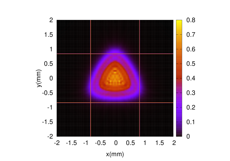
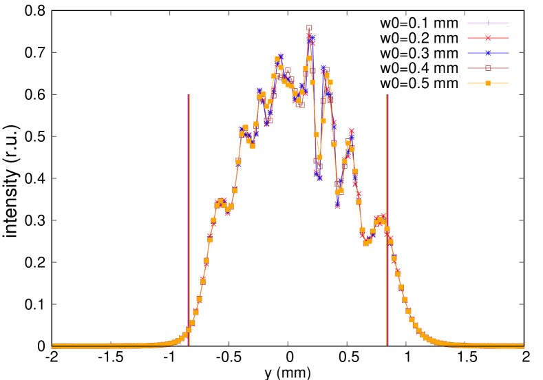
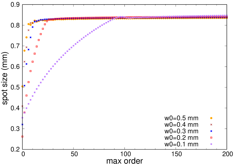
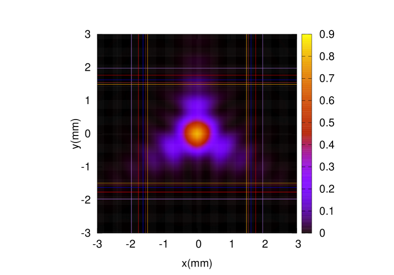
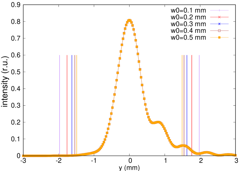
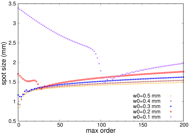
Figure 13: The intensity profiles of the simulated gaussian beam with aberration $\phi_{R}=Z_{3}^{-3}$ for the propagation distance $z=$100\text{\,}\mathrm{m}\mathrm{m}$$ (a) and $z=$1000\text{\,}\mathrm{m}\mathrm{m}$$ (d). The intensity distributions of the aberration beam along y-axis for the propagation distance $z=$100\text{\,}\mathrm{m}\mathrm{m}$$ (b) and $z=$1000\text{\,}\mathrm{m}\mathrm{m}$$ (e). The MSD spot size of the simulated aberration beam for different max mode order $N$ with the propagation distance $z=$100\text{\,}\mathrm{m}\mathrm{m}$$ (c) and $z=$1000\text{\,}\mathrm{m}\mathrm{m}$$ (f).

Appendix D The parameters of the MEM beam for the halo beam

The waist of the basic HG modes of the MEM beam for the halo beam is $w_{0}=$644.314\text{\,}\mu\mathrm{m}$$. The corresponding complex coefficients for different HG modes are shown in Appendix D. The HG modes in Appendix D are ordered in the absolute amplitude of complex coefficient $a_{mn}$ decreasingly.

complex coefficients for different HG modes of halo beam mode HG(m,n) complex coefficient $a_{mn}$ mode HG(m,n) complex coefficient $a_{mn}$ HG(0,0) 1.000000+0.000000i HG(1,2) -0.043850+0.030069i HG(0,2) -0.043689+0.208222i HG(5,4) -0.013644+0.044648i HG(0,8) 0.197328+0.079289i HG(7,1) 0.041697+0.015981i HG(2,0) 0.059580+0.202141i HG(2,3) 0.034655-0.027614i HG(8,0) 0.161853+0.090453i HG(4,5) 0.023136-0.037789i HG(6,0) 0.017052+0.166904i HG(3,6) -0.015738+0.037032i HG(7,0) -0.155352+0.053572i HG(1,8) -0.003275+0.039806i HG(2,6) 0.138949+0.064269i HG(5,3) 0.033787+0.016435i HG(4,4) 0.131712+0.067135i HG(3,2) -0.035438-0.009784i HG(0,6) -0.009895+0.144958i HG(4,1) 0.035344-0.005482i HG(0,4) 0.143830-0.009943i HG(3,5) 0.025634+0.022770i HG(6,2) 0.128264+0.065381i HG(6,3) 0.021603-0.024983i HG(0,7) 0.121691-0.062886i HG(0,11) -0.030008-0.013461i HG(4,2) -0.000903+0.128729i HG(1,5) -0.007792+0.030758i HG(2,4) -0.007101+0.123730i HG(1,7) 0.021235+0.020630i HG(0,10) 0.092926-0.069031i HG(9,1) 0.024615-0.015661i HG(4,0) 0.105540-0.014269i HG(5,1) 0.005574+0.027560i HG(0,9) 0.016402-0.104016i HG(3,3) 0.006984+0.025667i HG(0,3) 0.092075-0.035122i HG(8,1) 0.022251-0.014360i HG(5,2) -0.092037+0.034858i HG(1,4) -0.018101-0.014466i HG(2,2) 0.089174-0.014776i HG(11,0) 0.020614-0.010033i HG(2,5) 0.079592-0.040046i HG(7,3) 0.017058-0.014068i HG(9,0) -0.015792+0.087087i HG(1,10) 0.015733-0.000945i HG(3,0) -0.066284+0.043780i HG(1,9) 0.009205-0.011677i HG(3,4) -0.074522+0.020353i HG(5,5) 0.009195-0.005310i HG(10,0) 0.072191-0.022591i HG(3,7) 0.008557-0.001641i HG(2,8) 0.062475-0.038479i HG(3,1) 0.007785-0.001349i HG(4,6) 0.062011-0.034334i HG(2,9) -0.002583-0.007210i HG(5,0) -0.049725-0.043344i HG(6,5) 0.004232-0.005767i HG(6,4) 0.059852-0.026250i HG(1,1) 0.006285-0.001269i HG(4,3) 0.060351-0.023438i HG(3,8) 0.005092+0.001007i HG(1,6) -0.062262+0.016535i HG(5,6) 0.003077+0.002502i HG(2,7) 0.020276-0.058881i HG(10,1) 0.000208+0.003889i HG(6,1) 0.058091-0.010760i HG(1,3) -0.003512+0.000830i HG(8,2) 0.052511-0.025760i HG(4,7) -0.000359-0.003209i HG(2,1) 0.049257-0.030469i HG(9,2) -0.000481-0.003019i HG(0,5) 0.045250-0.033775i HG(8,3) 0.001417+0.001375i HG(7,2) -0.020618+0.052083i HG(7,4) -0.000059-0.000506i

Appendix E The parameters of the MEM beam for the Nearly-Gaussian beam II

The waist of the basic HG modes of the MEM beam for the Nearly-Gaussian beam II in Fig. 4 is $w_{0}=$399.465\text{\,}\mu\mathrm{m}$$. The corresponding complex coefficients for different HG modes are shown in Appendix E. The HG modes in Appendix E are ordered in the absolute amplitude of complex coefficient $a_{mn}$ decreasingly.

complex coefficients for different HG modes of Nearly-Gaussian beam II mode HG(m,n) complex coefficient $a_{mn}$ mode HG(m,n) complex coefficient $a_{mn}$ HG(0,0) 1.000000+0.000000i HG(8,0) -0.019123+0.021579i HG(2,0) 0.278731+0.219901i HG(1,6) -0.003373+0.028556i HG(0,2) -0.278731-0.219901i HG(1,8) 0.025500-0.011701i HG(7,0) 0.091524+0.172152i HG(1,5) 0.011388-0.025343i HG(5,0) 0.074602-0.159708i HG(8,1) 0.026540-0.005864i HG(0,4) 0.045154+0.159202i HG(6,4) 0.009602-0.024680i HG(2,2) -0.077211-0.129553i HG(4,6) 0.023531+0.011102i HG(3,0) -0.147112-0.019083i HG(6,1) -0.024231-0.004293i HG(4,0) -0.102501+0.088332i HG(3,5) 0.023611+0.005056i HG(9,0) -0.109524-0.077033i HG(0,5) -0.010220-0.020312i HG(6,0) 0.009151-0.097677i HG(5,6) -0.007497-0.021052i HG(7,2) 0.011396-0.087076i HG(2,8) -0.021737+0.002029i HG(1,1) -0.046646-0.072063i HG(3,6) -0.010431+0.017490i HG(4,2) 0.068784-0.051119i HG(0,11) -0.007996-0.016383i HG(5,2) -0.062910+0.053035i HG(5,5) -0.016094-0.005983i HG(2,4) 0.011725+0.073327i HG(9,1) 0.001334+0.016860i HG(0,6) 0.035398-0.063483i HG(6,3) 0.012951+0.010398i HG(11,0) 0.036618+0.061069i HG(7,3) -0.002000+0.015624i HG(3,2) 0.045392+0.043331i HG(4,1) 0.012962+0.007516i HG(1,3) 0.013945+0.055936i HG(1,10) -0.010509-0.010347i HG(4,4) -0.049109+0.017232i HG(2,7) -0.013172-0.002769i HG(1,2) 0.036656+0.036444i HG(2,5) 0.001213-0.013254i HG(5,4) 0.049164+0.001326i HG(4,3) -0.008941-0.009230i HG(6,2) -0.001349+0.044950i HG(10,1) -0.012455+0.002736i HG(2,6) 0.021935-0.038604i HG(2,1) 0.012290+0.002338i HG(3,4) -0.002739-0.040826i HG(2,3) 0.011532+0.001631i HG(9,2) 0.001930+0.040420i HG(1,7) -0.008886+0.005939i HG(3,1) 0.021898-0.029556i HG(8,3) -0.007374-0.006575i HG(0,7) -0.016107+0.032728i HG(2,9) 0.000048+0.009559i HG(0,9) 0.036413-0.001986i HG(3,7) 0.001158-0.009293i HG(1,4) -0.019041-0.029166i HG(0,10) 0.003370+0.008609i HG(5,1) 0.002507+0.033980i HG(4,5) 0.006450+0.005334i HG(3,3) -0.028347+0.016449i HG(8,2) -0.003821-0.004496i HG(7,4) -0.030367+0.009496i HG(3,8) 0.004060+0.001224i HG(10,0) 0.030037+0.008183i HG(6,5) 0.000037-0.003933i HG(5,3) 0.018109-0.024213i HG(0,3) 0.003511+0.001090i HG(7,1) -0.019281-0.022492i HG(1,9) 0.003354-0.000715i HG(0,8) -0.028999-0.001569i HG(4,7) -0.000144-0.003408i

References

- [1] L. D’Arcio, J. Bogenstahl, M. Dehne, C. Diekmann, E. Fitzsimons, R. Fleddermann, E. Granova, G. Heinzel, H. Hogenhuis, C. Killow, M. Perreur-Lloyd, J. Pijnenburg, D. Robertson, A. Shoda, A. Sohmer, A. Taylor, M. Tröbs, G. Wanner, H. Ward and D. Weise, Optical bench development for LISA, in Society of Photo-Optical Instrumentation Engineers (SPIE) Conference Series, , Society of Photo-Optical Instrumentation Engineers (SPIE) Conference Series Vol. 10565 (nov 2017), p. 105652X.
- [2] Z. Luo, Z. Guo, G. Jin, Y. Wu and W. Hu, Results in Physics 16 (Mar 2020) 102918.
- [3] W.-H. Ruan, C. Liu, Z.-K. Guo, Y.-L. Wu and R.-G. Cai, Nature Astronomy 4 (Feb 2020) 108, arXiv:2002.03603.
- [4] M. A. Porras, J. Alda and E. Bernabeu, Applied Optics 31 (Oct 1992) 6389.
- [5] A. E. Siegman, New developments in laser resonators, in Optical Resonators, ed. D. A. Holmes, Society of Photo-Optical Instrumentation Engineers (SPIE) Conference Series, Vol. 1224 (jun 1990), p. 2.
- [6] R. Martínez-Herrero, P. M. Mejías and M. Arias, Optics Letters 20 (Jan 1995) 124.
- [7] C. Paré and P.-A. Bélanger, Optics Communications 123 (Feb 1996) 679.
- [8] S. Amarande, A. Giesen and H. Hügel, Applied Optics 39 (Aug 2000) 3914.
- [9] E. M. Drège, N. G. Skinner and D. M. Byrne, Applied Optics 39 (2000) 4918.
- [10] A. E. Siegman, How to (Maybe) Measure Laser Beam Quality, in DPSS (Diode Pumped Solid State) Lasers: Applications and Issues, (OSA, Washington, D.C., 1998), p. MQ1.
- [11] S. N. Vlasov, V. A. Petrishchev and V. I. Talanov, Radiophysics and Quantum Electronics 14 (Sep 1971) 1062.
- [12] C. Bond, D. Brown, A. Freise and K. A. Strain, Living Reviews in Relativity 19 (Dec 2016) 3.
- [13] G. Wanner, G. Heinzel, E. Kochkina, C. Mahrdt, B. S. Sheard, S. Schuster and K. Danzmann, Optics Communications 285 (Nov 2012) 4831.
- [14] W. H. Carter, Applied Optics 19 (Apr 1980) 1027.
- [15] R. L. Phillips and L. C. Andrews, Applied Optics 22 (Mar 1983) 643.
- [16] R. Simon, N. Mukunda and E. Sudarshan, Optics Communications 65 (Mar 1988) 322.
- [17] M. A. Porras, Optics Communications 109 (Jun 1994) 5.
- [18] H. Weber, Optical and Quantum Electronics 24 (Sep 1992) S861.
- [19] G. A. Massey and A. E. Siegman, Applied Optics 8 (May 1969) 975.
- [20] J. Alda, Laser and Gaussian Beam Propagation and Transformation, 2nd editio edn. (CRC Press, sep 2015).
- [21] E. Kochkina, Stigmatic and astigmatic Gaussian beams in fundamental mode: impact of beam model choice on interferometric pathlength signal estimates, PhD thesis, Hannover: Gottfried Wilhelm Leibniz Universität Hannover (2013).
- [22] C. Braxmaier, G. Heinzel, K. F. Middleton, M. E. Caldwell, W. Konrad, H. Stockburger, S. Lucarelli, M. B. te Plate, V. Wand, A. C. Garcia, F. Draaisma, J. Pijnenburg, D. I. Robertson, C. Killow, H. Ward, K. Danzmann and U. A. Johann, LISA pathfinder optical interferometry, in Gravitational Wave and Particle Astrophysics Detectors, eds. J. Hough and G. H. Sanders, Society of Photo-Optical Instrumentation Engineers (SPIE) Conference Series, Vol. 5500 (sep 2004), p. 164.
- [23] X. Xue, H. Wei and A. G. Kirk, Journal of the Optical Society of America A 17 (Jun 2000) 1086.