Revisiting the composition dependence of the properties of water-dimethyl sulfoxide liquid mixtures. Molecular dynamics computer simulations

Abstract

We have revisited the composition dependence of principal properties of liquid water-DMSO mixtures by using the isobaric-isothermal molecular dynamics computer simulations. A set of non-polarizable semi-flexible models for the DMSO molecule combined with the TIP4P-2005 and TIP4P/$\varepsilon$ water models is considered. We restrict calculations to atmospheric pressure, 0.1013 MPa, and room temperature, 298.15 K. Composition trends of density, excess mixing volume and excess mixing enthalpy, partial molar volumes and partial molar enthalpies of species, apparent molar volumes are reported. Besides, we explore composition trends of the self-diffusion of species, the static dielectric constant and the surface tension. Evolution of the microscopic structure of the mixture with composition is analyzed in terms of radial distributions functions, coordination numbers and the fractions of hydrogen-bonded molecules. We intend to capture the peculiarities of mixing the species in the mixture upon the DMSO molar fraction and the anomalous behaviors, if manifested in each of the properties under study. The quality of several combinations of the models for species is evaluated in detail to establish the possibility of necessary improvements.

Key words: molecular dynamics, water-dimethyl sulfoxide mixtures, surface tension, dielectric constant, partial molar volumes, partial molar enthalpies

Abstract

Ó öié ðîáîòi ìè ïîâåðòàєìîñÿ äî ðîçãëÿäó êîíöåíòðàöiéíèõ çàëåæíîñòåé ãîëîâíèõ âëàñòèâîñòåé ðiäêèõ ñóìiøåé âîäà-ÄÌÑÎ ç âèêîðèñòàííÿì êîìï’þòåðíîãî ìîäåëþâàííÿ ìåòîäîì içîáàðèчíî-içîòåðìiчíî¿ ìîëåêóëÿðíî¿ äèíàìiêè. Ðîçãëÿíóòî íàáið íåïîëÿðèçîâíèõ íàïiâãíóчêèõ ìîäåëåé ìîëåêóë ÄÌÑÎ ó ïîєäíàííi ç ìîäåëÿìè âîäè TIP4P-2005 i TIP4P/$\varepsilon$. Îáчèñëåííÿ ïðîâåäåíî ïðè àòìîñôåðíîìó òèñêó 0.1013 MÏà òà êiìíàòíié òåìïåðàòóði 298.15 K. Íàâåäåíî êîíöåíòðàöiéíi çàëåæíîñòi ãóñòèíè, íàäëèøêîâîãî îá’єìó çìiøóâàííÿ, íàäëèøêîâî¿ åíòàëüïi¿ çìiøóâàííÿ, ïàðöiàëüíèõ ìîëÿðíèõ îá’єìiâ i ïàðöiàëüíî¿ ìîëÿðíî¿ åíòàëüïi¿ ñêëàäíèêiâ ñóìiøi, âèäèìèõ ìîëÿðíèõ îá’єìiâ. Òàêîæ äîñëiäæåíî êîíöåíòðàöiéíi çàëåæíîñòi ñàìîäèôóçi¿ ñêëàäíèêiâ, ñòàòèчíî¿ äiåëåêòðèчíî¿ ñòàëî¿ òà ïîâåðõíåâîãî íàòÿãó. Çìiíè ìiêðîñêîïiчíî¿ ñòðóêòóðè ñóìiøi â çàëåæíîñòi âiä ¿¿ ñêëàäó ïðîàíàëiçîâàíî íà îñíîâi ðàäiàëüíèõ ôóíêöi¿ ðîçïîäiëó, êîîðäèíàöiéíèõ чèñåë òà чàñòîê ìîëåêóë, ïîâ’ÿçàíèõ âîäíåâèìè çâ’ÿçêàìè. Ìåòîþ є çàôiêñóâàòè îñîáëèâîñòi çìiøóâàííÿ ñêëàäíèêiâ ñóìiøi ïðè çìiíi ìîëÿðíî¿ чàñòêè ÄÌÑÎ, à òàêîæ ìîæëèâi àíîìàëi¿ äîñëiäæåíèõ õàðàêòåðèñòèê. Ïðîâåäåíî îöiíêó ïðèäàòíîñòi ðiçíèõ êîìáiíàöié ìîäåëåé ñêëàäíèêiâ ñóìiøi äëÿ òîãî, ùîá ç’ÿñóâàòè íåîáõiäíiñòü ó ïîäàëüøîìó âäîñêîíàëåííi.

Ключовi слова: ìîëåêóëÿðíà äèíàìiêà, ñóìiøi âîäà-äèìåòèëñóëüôîêñèä (ÄÌÑÎ), ïîâåðõíåâèé íàòÿã, äiåëåêòðèчíà ñòàëà, ïàðöiàëüíi ìîëÿðíi îá’єìè, ïàðöiàëüíi ìîëÿðíi åíòàëüïi¿

1 Introduction

Liquid mixtures of dimethyl sulfoxide (DMSO) and water are of much practical importance as solvents and reaction media in organic chemistry and chemical engineering [1, 2, 3]. Besides, they are widely used in several biological applications, cryoprotection being just one example, see e.g., [4, 5, 6].

Thus, it is not only desirable but also necessary to have an accurate description of various properties of these mixtures dependent on composition, $X$, temperature, $T$, and pressure, $P$. Common experimental practice is to study the composition effects at a room temperature and not far from it. Moreover, in many studies the atmospheric pressure is assumed. Much less studies are focused on temperature and pressure trends of the behavior of water-DMSO liquid mixtures. Unfortunately, experimental results do not cover all the cases of interest. In other words they do not provide comprehensive knowledge about the dependence of even some basic properties of the system in question, upon changes of these thermodynamic variables. As documented in reference [7], the experimental knowledge and understanding of the microscopic structure and dynamic properties of the systems in question mainly follows from the application of neutron scattering, nuclear magnetic resonance, dielectric relaxation and vibrational spectroscopy methods. In order to interpret the experimental observations in detail and to get ampler insights, one is forced to resort to computer simulations methodology.

Usual strategy of computer simulations methodology is to choose a model of each species, water and DMSO in the present case, and assume the cross interactions by using the combination rules. Then, a software based on strict rules of statistical mechanics is applied. Adequacy of the computer simulations predictions for a given model for solution, upon changing $X,T$ and $P$, is then tested by comparison with some reference experimental data. Afterwards, the profit of the method is in the possibility to interpret these observables at microscopic level with molecular level details. Besides, it becomes possible to explore a wider set of properties, in addition to the benchmark or reference experimental data, with a reasonable degree of confidence. It is worth to mention that the trajectories of particles generated by molecular dynamics (MD) simulations provide two types of results. Namely, one of them includes “direct” properties, e.g., the equation of state in terms of density at a given temperature and pressure upon changing composition in the NPT ensemble, enthalpy, $H(T,P,X)$, a set of radial distribution functions of particles and the self-diffusion coefficients of species. On the other hand, another type of properties follows from the time averages of fluctuations. These are, for example, the isothermal compressibility and the dielectric constant. The latter are more sensitive to the number of particles in the principal simulated volume, to the time extension of the simulations and to the method of account for the long-range contribution of inter-particle interactions.

Having this in mind, the principal objective of the present work is to revisit the composition trends of the behavior of water-DMSO mixtures at atmospheric pressure and room temperature by using isobaric-isothermal molecular dynamics computer simulation. The reason is that several previous publications were focused on elucidation of anomalies of composition behavior, or better say of non-monotonous behaviors of different properties and their interpretation from molecular dynamics simulations. Some sets of experimental data permit to obtain anomalies straightforwardly. On the other hand, hidden anomalies from apparently monotonous behavior can be extracted as well. We would like to show that confidence into the presence of anomalies coming from computer simulations results requires a very good description of the underlying properties with respect to experimental data. Otherwise, the anomalies resulting from the analyses of computer simulations results may follow from the behavior of a model rather than from reality.

The first MD simulations of systems of our interest were reported in [8, 9, 10, 11]. In order to formulate the force fields, the experimental observations and quantum chemical calculations were used. Further refinement of parameters was performed in some cases by minimizing the differences of model calculations with a few experimental observables. Concerning the nomenclature and parameters of the DMSO models most frequently used in the literature, we refer to the Table I in each of the references [10, 12, 13], as well as to the table 2 of reference [14]. Enormous set of results concerning structure and thermodynamics, dynamics and dielectric properties was generated  [8, 9, 10, 11, 12, 13, 14, 15, 16, 17, 18, 19, 20, 21, 22, 23, 24].

At present, the most widely used models for the DMSO are at the united atom level (DMSO-UA); in this framework, each methyl group is considered as a single site. Nevertheless, the attempts to improve the description of the properties of pure DMSO and water-DMSO mixtures, by using either flexible or all-atom or simple polarizable DMSO models were undertaken [12, 25, 26, 27, 28, 29, 30, 31]. The majority of the MD studies for the united atom models were performed at NVT conditions using experimental densities for different compositions  [8, 9, 10, 15, 19] or by means of NVE simulations [12, 14, 16, 17]. The isobaric-isothermal (NPT) setup was employed as well [18, 20, 22, 23, 26, 32, 33]. In a comprehensive study of excess mixing properties of water-DMSO model mixtures at room temperature and atmospheric pressure, the NVT Monte Carlo technique was applied [13]. A peculiar behavior reflecting the hydrophobic effect in such mixtures was explored in [20, 22]. To summarize, the overwhelming body of computer simulation results refers to composition changes of the properties for the system in question rather than to temperature and/or pressure effect. Finally, it is worth mentioning that the solvation of complex molecules in water-DMSO mixtures was the subject of several simulations and experimental studies, see e.g., references [34, 35, 36, 37, 38, 39].

2 Models and simulation details of the present work

In this work we restrict our attention to a few DMSO united atom type, non-polarizable models with four sites, O, S, CH₃ (methyl group carbon and hydrogens interaction sites are replaced by a single CH₃ site located on the methyl carbon atom). Within this type of modelling, the interaction potential between all atoms and/or groups is assumed as a sum of Lennard-Jones (LJ) and Coulomb terms. A comprehensive description of the parameters of models of this type is given in table 1 of [40] and in table 1 of [13]. In all cases, the models are considered as rigid. Some basic properties under specific conditions concerned with computer simulations setup are also reported in table 2 of [40]. A set of parameters for each model follows from fitting to a few target properties, e.g., the heat of vaporization and charge distribution in order to yield a dipole moment of the molecule in the gas phase, which is the case to construct for example the P2 model for DMSO [10]. Experimental predictions for the intra-molecular structure and auxiliary ab initio calculations were used in the design of DMSO models as well. Several attempts to better describe a wider set of target properties of DMSO at ambient conditions were undertaken via parametrization of charges and LJ parameters still keeping the model rigid [11, 15, 32]. In order to improve the rigid P2 model, Benjamin proposed to include the effects of intra-molecular flexibility [28]. The parameters for intra-molecular potential describing harmonic bonds and angles were chosen to reproduce the gas phase normal mode frequencies. It was shown however [29], that the model essentially overestimates the liquid DMSO density at room temperature. Thus, it is improbable to expect a good level description of the density of water-DMSO mixtures over the entire composition range.

Both rigid or flexible DMSO model can also be constructed by using a well established OPLS database [41]. The OPLS and P1 and P2 models [10] are characterized by identical molecular geometry, though the LJ parameters are different. The site charges are the same for the OPLS and P2 models. In the construction of a flexible model, one can take parameters from the OPLS database. However, to keep the molecular geometry, it is then recommended to complement the DMSO model by the improper dihedral angle S–C–O–C see reference [42].

In the present study we apply the DMSO united atom models with four sites, O, S, CH₃. The CH₃ is abbreviated as C in what follows. The models are non-polarizable and denominated as P1, P2  [10] and OPLS (see e.g., table II of reference [43]). The interaction potential between all atoms and/or groups is a sum of Lennard-Jones (LJ) and Coulomb terms. All the parameters are given in table 1 for the sake of convenience of the reader. In addition, after testing several possibilities, we assumed C–S and S–O bonds rigid whereas the O–S–C and C–S–C are chosen flexible, the harmonic constant is taken from the OPLS database. Moreover, the improper dihedral S–C–O–C is included into the DMSO models. The parameters are taken from reference [42]. Our tests indicate that this element is crucial to yield a reasonable value for pure DMSO liquid density in each of the models involved in this study. In summary, we applied semi-flexible models for DMSO molecule.

Table 1: Lennard-Jones parameters for the P1, P2 and OPLS models of dimethylsulfoxide. All $\sigma$ are in Å, $\varepsilon$ — in kJ/mol and charges, $q$, in $e$ units. All models assume the O–S–C angle at 106.75^∘ and the C–S–C angle at 97.4^∘. The charges are: $q_{\rm{O}}=-0.459$, $q_{\rm{S}}=0.139$ and $q_{\rm{C}}=0.160$ for P2 and OPLS models. In the case of P1 model, the charges are: $q_{\rm{O}}=-0.54$, $q_{\rm{S}}=0.54$ and $q_{\rm{C}}=0$.

Model	$\varepsilon_{\rm{OO}}$	$\sigma_{\rm{OO}}$	$\varepsilon_{\rm{SS}}$	$\sigma_{\rm{SS}}$	$\varepsilon_{\rm{CC}}$	$\sigma_{\rm{CC}}$
P1	0.2992	2.80	0.9974	3.40	1.230	3.80
P2	0.2992	2.80	0.9974	3.40	1.230	3.80
OPLS	1.171	2.93	1.652	3.56	0.669	3.81

For water, the TIP4P-2005 model was applied [44]. In many cases we used the TIP4P/$\varepsilon$ model [45] as well. It was designed to improve the inadequacy of the prediction of the static dielectric constant of water by TIP4P-2005. Lorentz-Berthelot combination rules were used to determine the cross parameters for the relevant potential well depths and diameters for the P1-water and P2-water models, whereas the geometric combination rule was assumed for the OPLS-TIP4P-2005 model.

Molecular dynamics computer simulations of DMSO-water mixtures were performed in the isothermal-isobaric (NPT) ensemble at atmospheric pressure 1 bar and at temperature 298.15 K. We used GROMACS package [46] version 5.1.2. The simulation box in each run was cubic, the total number of molecules of both species is fixed at 3000. Composition of the mixture is described by the molar fraction of DMSO molecules, $X_{d}=N_{d}/(N_{d}+N_{w})$. As common, periodic boundary conditions were used. Temperature and pressure control was provided by the V-rescale thermostat and Parrinello-Rahman barostat with $\tau_{T}=0.5$ ps and $\tau_{P}=2.0$ ps, the timestep was 0.001 ps. The value of $4.5\times 10^{-5}$ bar^-1 was used for the compressibility of mixtures.

The non-bonded interactions were cut-off at 1.1 nm, whereas the long-range electrostatic interactions were handled by the particle mesh Ewald method implemented in the GROMACS software package (fourth order, Fourier spacing equal to 0.12) with the precision $10^{-5}$. The van der Waals correction terms to the energy and pressure were applied. In order to maintain the geometry of water molecules and DMSO intra-molecular bonds rigid, the LINCS algorithm was used.

After preprocessing and equilibration, consecutive simulation runs, each for not less than 10 ns, with the starting configuration being the last configuration from the previous run, were performed to obtain trajectories for the data analysis. The results for each property were obtained by averaging over 7–10 production runs.

3 Results and discussion

3.1 Density of water-DMSO mixtures on composition

As we mentioned in the introductory section, there were several experimental reports concerning the evolution of density of DMSO-water mixtures upon changing composition. We used experimental data by Egorov and Makarov at room temperature $T=298.15$ K, and atmospheric pressure [47].

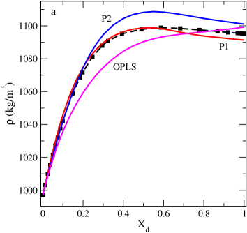
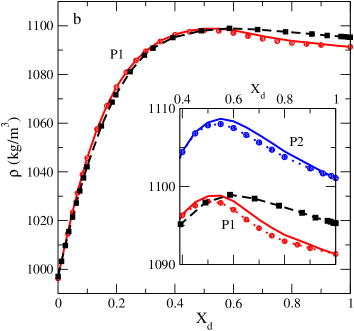
Figure 1: (Colour online) Panel a: composition dependence of the density of water-DMSO mixtures from the NPT MD simulations of P1-TIP4P-2005 model (solid red line), P2-TIP4P-2005 model (solid blue line) and OPLS-TIP4P-2005 model (solid magenta line) in comparison with the experimental data (dashed lines with squares) at 298.15 K [47]. Panel b: similar to the panel a but for P1-TIP4P-2005 model (solid red line), P1-TIP4P/$\varepsilon$ water model (solid circles). The inset gives an enhanced view of the effects of substitution of TIP4P-2005 (lines) by TIP4P/$\varepsilon$ (circles) water model if the P1 and P2 models for DMSO are used. Experimental data are from  [47].

The experimental data at $T=298.15$ K witness that the density of water-DMSO mixtures increases quite rapidly with $X_{d}$ starting from pure water density ($997$ kg/m³) and reaches a weakly pronounced maximum around $X_{d}\approx 0.6$. Next, with a further increase of $X_{d}$, i.e., in the interval where the DMSO amount within the mixture predominates, the density slightly decreases with $X_{d}$ and reaches the pure liquid DMSO density, $\rho=1095$ kg/m³, figure 1 (panel a). It is reasonable to interpret the presence of a maximum density along the composition axis as an evidence of the stronger water-DMSO interaction, compared to the water-water inter-molecular interaction  [47].

Molecular dynamics computer simulation results for P1, P2 and OPLS DMSO models combined with TIP4P-2005 water model in the entire composition range are given in figure 1 a by red, blue and magenta lines, respectively. We observe that qualitative trends of behavior of density on composition are correctly reproduced by the P1-TIP4P-2005 and P2-TIP4P-2005 models. The maximum of density from simulations of these models is captured. Moreover, the growth and decay of density in the interval of compositions with small DMSO amount and in the interval of small water concentrations, respectively, are reproduced by both models as well. By contrast, the OPLS-TIP4P-2005 model predicts a monotonous growth of the mixture density with an increasing $X_{d}$ in the entire composition interval. Thus, the simulations of all model combinations show that the density increases upon adding foreign species to water. If water is added to pure DMSO solvent, P1 and P2 predict a growth of density. The OPLS model leads to an opposite trend, it yields a decreasing density, or in other words at constant pressure the volume of principal simulation box increases. If water enters DMSO structure within P2 or P1 models, the attraction dominates, then the density increases. On the other hand, if water enters the “sea” of OPLS molecules, repulsion prevails and consequently the box increases or equivalently the density decreases.

The P2-TIP4P-2005 model works very well up to $X_{d}\approx 0.2$. For this interval of composition, the performance of the P1-TIP4P-2005 model is very satisfactory as well. On the other hand, at higher values of $X_{d}$, the P2-TIP4P-2005 model overestimates the density of mixtures as the result of overestimation of pure DMSO liquid density. By contrast, the P1 model slightly underestimates the density of pure liquid DMSO. Consequently, the density of water-DMSO mixtures is slightly underestimated at high $X_{d}$. In fact, this deviation in both cases is not too big. It is of the order of one percent w.r.t. experimental value. If the TIP4P-2005 water model is substituted by the TIP4P/$\varepsilon$ model, the situation remains almost the same. In panel b of figure 1, we compare performance of the P2 model for DMSO combined with two water models w.r.t. experimental data. The inset to panel b of figure 1 shows a marginal deviation of the mixture density upon changing the water model. Furthermore, the inset shows that the maximum density from simulations [$X_{d}\approx 0.55$ is close to its experimental counterpart ($X_{D}\approx 0.58$)]. In summary, the dependence of density on composition with a single peculiar point is quite accurately described by two, P1 and P2, DMSO models if combined with either TIP4P-2005 or TIP4P/$\varepsilon$ models, whereas the OPLS-TIP4P-2005 model does not capture this behavior.

3.2 Excess mixing volume, partial molar and apparent molar volumes of species on composition

However, it is of importance not only to describe the trends of behavior of the given property on composition, but to correctly capture the deviation from ideality as well. These insights follow from the behavior of the excess density or the excess mixing volume, for example. The excess mixing volume is defined as follows, $\Delta V_{\rm{mix}}=V_{\rm{mix}}-X_{d}V_{d}-(1-X_{d})V_{w}$, where $V_{\rm{mix}}$, $V_{d}$ and $V_{w}$ refer to the molar volume of the mixture and of the individual components, DMSO and water, respectively.

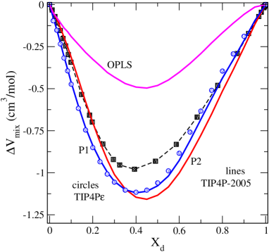
Figure 2: (Colour online) A comparison of the composition dependence of the excess mixing volume of water-DMSO mixtures for different DMSO (P1, P2 and OPLS) models with the experimental data of reference [47]. In addition, the effect of substitution of TIP4P-2005 (blue line) by TIP4P/$\varepsilon$ (blue circles) water model is shown. The results refer to 298.15 K and atmospheric pressure.

In order to elucidate the composition trends of the behavior of the excess mixing volume, we plot the simulation results and experimental data at 298.15 K in figure 2. Experimental data show that $\Delta V_{\rm{mix}}$ is negative and exhibit a minimum at $X_{d}\approx 0.4$. The simulation results qualitatively show similar trends of behavior. The values for $\Delta V_{\rm{mix}}$ are just slightly overestimated at intermediate compositions, if P1-TIP4P-2005 or P2-TIP4P-2005 models are used. At low $X_{d}$ values, the P2-TIP4P-2005 model performs better than P1-TIP4P-2005 model. However, the P1-TIP4P-2005 model predicts the location of $\Delta V_{\rm{mix}}$ a bit better than the P2-TIP4P-2005. Also for high $X_{d}$ values, P1-TIP4P-2005 is better than P2-TIP4P-2005. The OPLS-TIP4P-2005 essentially underestimates the excess mixing volume in the entire composition interval. Thus, a comparison between the experiment and simulations of P1 and P2 models with either TIP4P-2005 or TIP4P/$\varepsilon$ can be termed as quite satisfactory concerning the geometric aspects of mixing of species. In this projection of the equation of state for DMSO-water mixture, we observe a single peculiar point on composition in close similarity to the behavior of density, as expected.

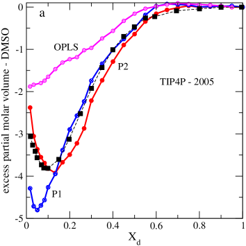
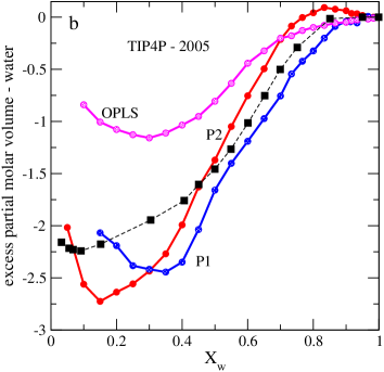
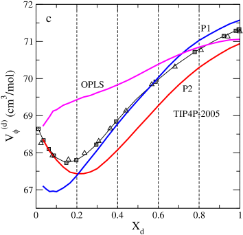
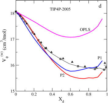
Figure 3: (Colour online) Panels a and b: a comparison of the composition dependence of the excess partial molar volumes of DMSO and of water from simulations, with the experimental data (squares reference [49]) at 298.15 K. Panels c and d: a comparison of the composition dependence of the apparent molar volumes of DMSO and of water from simulations, with the experimental data (squares reference [47] and triangles reference [50]) at 298.15 K.

The maximum deviation from the ideal mixing at $X_{D}\approx 0.4$ is interpreted as trends for the formation of “complexes” or “associates” of the 2DMSO-3H₂O type [18]. On the other hand, it is documented that the maximum deviation from ideality of density and of other properties on composition can be characterized in terms of percolation phenomena [48].

In order to discern the contribution of each species of the mixture into the mixing volume, it is common to resort to the excess partial molar volumes. They are defined as, $\overline{V^{ex}_{i}}=\overline{V}_{i}-V_{i}$, where $\overline{V}_{i}$ denotes the partial molar volume of species $i$ ($w$ or $d$). The partial molar volumes result from the excess mixing volume, $\Delta V_{\rm{mix}}$ as follows [49],

$$\overline{V}_{w}=\Delta V_{\rm{mix}}+V_{w}+X_{d}\left(\frac{\partial\Delta V_{\rm{mix}}}{\partial X_{w}}\right)\bigg{|}_{P,T},$$ (3.1)

$$\overline{V}_{d}=\Delta V_{\rm{mix}}+V_{d}-X_{w}\left(\frac{\partial\Delta V_{\rm{mix}}}{\partial X_{w}}\right)\bigg{|}_{P,T},$$ (3.2)

where $X_{w}=1-X_{d}$. The excess partial molar volumes of DMSO and water species are plotted in the panels a and b of figure 3. The experimental data are taken from figures 5 and 6 of reference [49]. The best agreement with the experimental results for $\overline{V^{ex}_{d}}$ is obtained for the P2-TIP4P-2005 model. Namely, the shape of the curve and the minimum for $\overline{V^{ex}_{d}}$ are reproduced quite well. Predictions from the P1-TIP4P-2005 model are reasonable as well. However, the location and the value for the minimum are less accurate in comparison to P2-TIP4P-2005 model. Concerning the predictions of different models w.r.t. the $\overline{V^{ex}_{w}}$, the situation is a bit worse. Both models, the P2-TIP4P-2005 and P1-TIP4P-2005, describe the behavior of the excess partial molar volume well at a high water content. On the other hand, for DMSO-rich mixtures, the simulation data deviate from the experimental results. The experimental data show that the minimum of $\overline{V^{ex}_{w}}$ is weakly pronounced and is located at $X_{w}\approx 0.1$. By contrast, the simulation data predict much stronger pronounced minimum at a higher water content. In summary, the dissolution of water species in the DMSO solvent is not accurately described. The worse predictions for $\overline{V^{ex}_{d}}$ and $\overline{V^{ex}_{w}}$ come out from the application of the OPLS-TIP4P-2005 model.

Similar insights into the geometric aspects of mixing on composition, both from experiments and simulations, can be obtained by resorting to the notion of the apparent molar volume of species rather than the partial molar volumes. The apparent molar volume for each species [49] according to the definition is: $V_{\phi}^{(w)}=V_{w}+\Delta V_{\rm{mix}}/(1-X_{d})$ and $V_{\phi}^{(d)}=V_{d}+\Delta V_{\rm{mix}}/X_{d}$. We elaborated the experimental density data from references [47, 50] and the results from our simulations to construct the plots shown in panels c and d of figure 3. These plots confirm that the P2-TIP4P-2005 model provides a reasonable description of the composition behavior for $V_{\phi}^{(d)}$ in water-rich mixtures while the P1-TIP4P-2005 model is satisfactory for DMSO-rich mixtures.

This kind of composition behavior of apparent molar volumes of DMSO species in water-rich mixtures can be related to the experimental results for abnormal intensity of scattered light [51]. The minimum of the apparent molar volume of DMSO indicates the hydrophobic effect in the systems in question due to enhanced concentration fluctuations within certain composition interval.

3.3 Energetic aspects of mixing of DMSO and water molecules

Next, we proceed to the energetic manifestation of mixing trends. The experimental data are scarce in this aspect, we used the results from references [52, 53, 54, 55] to explore the mixing enthalpy upon composition of the water-DMSO mixtures.

To begin with, the simulation results for the enthalpy on composition for different combinations of models are given in panel a of figure 4. The curves resulting from P2-TIP4P-2005 and P1-TIP4P-2005 predict the presence of a minimum at $X_{d}\approx 0.35$ and at 0.45, respectively. By contrast, the OPLS-TIP4P-2005 does not predict the existence of the minimum for $H(X_{d})$. If one applies the TIP4P/$\varepsilon$ model rather than the TIP4P-2005 model, the absolute values of enthalpy increase and the minimum shifts to a lower DMSO concentration.

The experimental results, however, refer to the excess mixing enthalpy rather that to the absolute values. It follows from the results shown in panel b of figure 4, that the P1 and P2 DMSO models combined with the TIP4P-2005 water substantially over-predict the mixing enthalpy. Changing the water model from TIP4P-2005 to TIP4P/$\varepsilon$ does not yield an improvement in the considered aspect. This seems to be a quite general failure of a set of non-polarizable water and DMSO combinations of models as documented in the comprehensive study [13], see figures 3 and 5 of that reference. On the other hand, from our figure 4 b, we observe that the OPLS-TIP4P-2005 model underestimates the mixing enthalpy but the results are not far from the experimental points. The excess partial molar enthalpies can be obtained by using equations (3.1) and (3.2), just the volume should be substituted by enthalpy. The agreement between the experimental data and predictions of a set of models in question can be termed as qualitative and in some cases as quantitative for water-rich or DMSO-rich mixtures. The OPLS-TIP4P-2005 model yields the most reasonable coincidence with the experimental data. However, the energetic aspects of mixing of species, in terms of $\overline{H^{ex}_{w}}$ and $\overline{H^{ex}_{d}}$ simultaneously, are better described for water-rich mixtures.

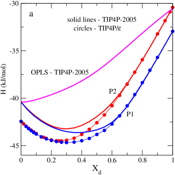
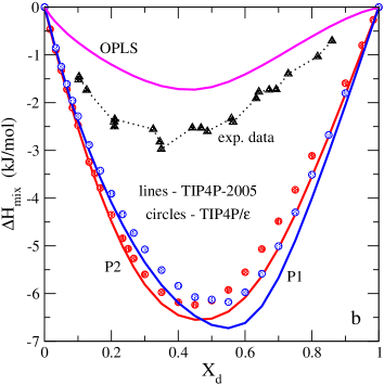
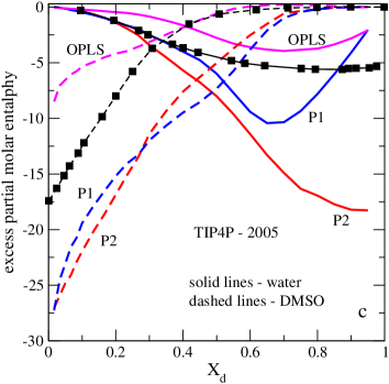
Figure 4: (Colour online) Panel a: composition dependence of enthalpy of water-DMSO mixtures at 298.15 K for different combinations of DMSO and water models. Panel b: a comparison of the behavior of the excess mixing enthalpy from simulations of different models and experimental data from reference [52]. The nomenclature of lines and symbols is given in the figure. Panel c: excess partial molar enthalpies of species on composition from simulations. The experimental data are from Lai et al. [54].

3.4 Comments on the evolution of the microscopic structure upon changes of composition

In all the above discussion concerned with geometric and energetic aspect of mixing of water and DMSO species from molecular dynamics computer simulations of different models, we have intended to validate the theoretical predictions w.r.t. experimental results in every detail. One of well established observations is in the existence of the minimum of the excess partial molar volume or of the apparent molar volume of DMSO species at a low $X_{d}$. This specific interval of composition is the subject of search of anomalous behavior of different properties in references [20, 22, 34]. Some insights in those works were obtained from the analysis of the microscopic structure.

Without referring directly to experimental results, it is difficult to prove that the computer simulation predictions for the microscopic structure of the mixtures in question are reasonable. Recently, the contributions of our collaborators [56, 57] have scrutinized this problem for pure water and water-methanol mixtures. Unfortunately, we are not aware of comprehensive experimental measurements of the total and partial structure factors in the entire composition interval for water-DMSO mixtures. Thus, the discussion below should be considered as mirror interpretation of thermodynamic results given above, rather than as independent and confident source to capture possible anomalous behaviors.

Consequently, we would like to perform mere analyses of the structural motifs by considering how the partial radial distribution functions change upon adding the DMSO molecules to water. The results are presented in the following figures. We restrict principally to the results for P2-TIP4P-2005 model because it provides the best description of the density dependence on composition and of other properties of water-rich mixtures, as documented above.

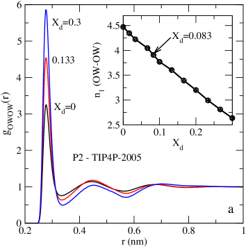
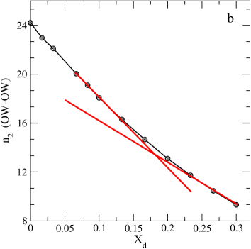
Figure 5: (Colour online) Panel a: composition dependence of the radial distribution functions of water oxygens for P2-TIP4P-2005 model in water-rich mixtures. Inset: the first coordination number on DMSO concentration. Panel b: evolution of the second coordination number upon mixture composition.

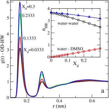
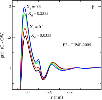
Figure 6: (Colour online) Composition dependence of the cross radial distribution functions between atoms of DMSO and water molecules. The inset to panel a shows changes of the average number of hydrogen bonds per water molecule between water molecules (black circles), between water and DMSO molecules (red circles) and their sum (blue triangles).

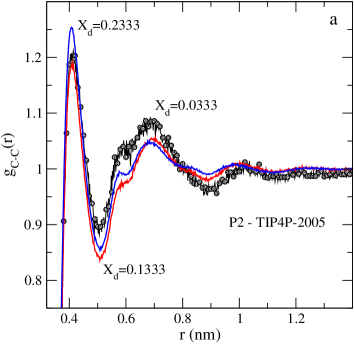
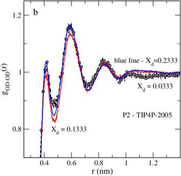
Figure 7: (Colour online) Composition dependence of the radial distribution functions of selected species for P2-TIP4P-2005 model in water-rich mixtures.

We observe that some of the functions exhibit anomalous changes whereas the other functions change monotonously. Specifically, the radial distribution function for water oxygens in given in figure 5. The first maximum of this function grows in magnitude with an increasing DMSO concentration. This growth is accompanied by a decrease of the height of the second maximum. Moreover, the location of the first maximum along $r$-axis does not change with $X_{d}$, whereas the following oscillations slightly shift to larger distances. These changes can be characterized by the first (inset to panel a) and the second (panel b) coordination numbers evaluated by integration to the respective minimum of the $g(r)$ as common,

$$n_{i}(r)=4\piup\rho_{j}\int_{0}^{r_{\rm{min}}}g_{ij}(R)R^{2}\mathrm{d}R,$$ (3.3)

where $\rho_{j}$ is the density of species $j$.

This kind of evolution of $g(r)$ for water species in water-DMSO mixtures was discussed already in reference [10] (figure 7 of  [10]) and in reference [33]. In addition to previous observations, we would like to note that the first coordination number exhibits a weak nonlinearity as shown in the inset to figure 5. Besides, we observed that the second coordination number changes its shape on $X_{d}$ at $X_{d}\approx 0.1667$ as a reflection of changes of the second maximum of $g(r)$ for water oxygens. A narrow range of compositions around this value is analyzed in [20] suspecting an anomalous behavior of the number of contacts between methyl groups of DMSO molecules in water-rich mixtures, cf. figures 8 and 9 of reference [20]. In summary to figure 5, we note that the behavior of $g(r)$ for OW-OW can be interpreted as the enhancement of the short-range structure of water upon adding the DMSO species. On the other hand, trends for a weaker structure at larger separations between water molecules witness that on a larger scale, hydrogen bonded network of water becomes dismantled. Nevertheless, the entire interval of composition considered in figures 5 and 6 refers to systems with a rather high degree of hydrogen bonding. The average number of hydrogen bonds (per water molecule) between species of the mixture is illustrated in the inset to figure 6. We used GROMACS software with default parameters to obtain the data. The average number of H-bonds between water molecule drops down from 3.7 to 2.5 within the $X_{d}$ interval considered. On the other hand, the bonds are formed upon DMSO insertion into water medium, such that their sum, or say bonding state of water molecules, remains almost as high as in pure water. We have not elaborated the H-bonding structure of the systems in question more in detail, however. Certain additional details can be deduced by using a previous observation for our laboratory, see e.g., figure 8 and 9 of reference [33]. It is worth to extend the study of these issues by involving the energetic definition of hydrogen bonding, see e.g., [58], and by searching for the elements of microscopic structure due to cooperativity of hydrogen bonds in the spirit of reference [59]. The hydrogen bonds lifetime should be explored as well.

Some aspects of the structural arrangement of different species in water-DMSO mixtures upon increasing the DMSO concentrations are illustrated in figure 6. The principal effect is shown in panel a of this figure. Namely, the probability of finding water hydrogens close to the oxygens of DMSO molecules substantially increases with an increasing $X_{d}$. The second maximum increases as well. The first maximum is observed at the same OD-HW distance upon increasing $X_{d}$. Thus, this structure reflects the formation of hydrogen bonds between DMSO and water molecules. The second maximum, presumably corresponds to the second shell of water molecules bonded to molecules of the first shell around the “reference” oxygen of DMSO molecule. At larger distances, the distribution function remains almost flat. A quite similar shape of this function was documented previously at $X_{d}=0.35$, cf. figure 3 of reference [10].

Because of bonding discussed just above, the distribution function of water oxygens w.r.t. methyl groups exhibits similar trends, panel b of figure 6. Its first maximum increases with increasing $X_{d}$. However, the second maximum remains constant and then decreases in magnitude when the DMSO concentration increases. Note that both maxima are observed at the distances larger than the first and the second maximum of OD-HW distribution in panel a, as expected.

The pair distribution functions describing the changes of distribution of methyl groups, C-C (the inter-molecular part) and of OD-OD behave differently, in comparison to our discussion above. They are plotted in figure 7. Namely, the first maximum of the radial distributions shown in panels a and b decreases in magnitude when $X_{d}$ increases from $0.0333$ up to $0.1333$. Next, the first maximum of both functions grows, if $X_{d}$ increases further, up to $0.2333$. The magnitude of the second maximum exhibits similar trends. The shape of the functions from our calculations favourably compares to the ones obtained in [10] by using the P1 and P2 models combined with the SPC water model, cf. figures 1 and 4 of that reference.

However, the radial distribution functions of methyl groups require additional comments because it should reflect possible aggregation of hydrophobic methyl groups. In order to get more detailed insights into the behavior of this function, we elaborated figure 8 a by using the OPLS-TIP4P-2005 model for mixtures in question. The shape of the curves differ from what we obtained for P2-TIP4P-2005 model in figure 7 a. However, in qualitative terms, the C-C function from the OPLS-TIP4P-2005 model is very similar to the result of Bagchi et al. in reference [20] using another force field, cf. figure 6 of  [20].

We used additional descriptors to characterize the distribution function of methyl groups. Namely, we calculated the first coordination number of the distribution of a single methyl group of a DMSO molecule, figure 8 b, using the P2-TIP4P-2005 and OPLS-TIP4P-2005 model. Apparently, both curves are smooth without any discontinuity. The inclination of the curve coming from OPLS-TIP4P-2005 model continuously changes in the composition interval between 0.1 and 0.2. The “crossover” between parts of the function on the DMSO concentration can be estimated at $X_{d}$ = 0.15. A similar value for a peculiar composition was obtained in reference [20] from the analyses of the total fraction of contacts between methyl groups on composition and of the average number of methyl groups around a given group (see figures 9 and 10 in reference [20]). However, these authors claimed to observe a discontinuous transition termed as weak transition between two regimes, in contrast to our observations. A similar curve coming from the calculations for P2-TIP4P-2005 is given in figure 8 b as well. In this case, there is a very weakly pronounced change of the inclination of the curve between $X_{d}$ = 0.1667 and 0.2. However, it can hardly be interpreted as a pronounced discontinuity.

We would like to finish this part by recalling that the predictions of the OPLS-TIP4P-2005 model for density, for the excess mixing volume and related partials as well as for energetic aspects of mixing of species are not satisfactory. Therefore, it does not seem consistent to discuss anomalous behaviors by using solely certain aspects of microscopic structure from a particular model force field that leads to a quite inaccurate thermodynamic and other properties. Evidently, our comments concerning the microscopic structure are not comprehensive. It would be desirable to validate the structure by comparison with the experimental predictions for the structure factors in the entire composition range. Unfortunately, as it was mentioned at the beginning of this subsection, such data are not available in the literature, up to our best knowledge.

In contrast to microscopic structure, there are different possibilities to validate the force field models against the experimental data. One of the possibilities is to discuss the dynamic properties. Most common, computer simulations predictions are confronted with the experimental results for self-diffusion coefficients of species upon the composition of the solutions in question.

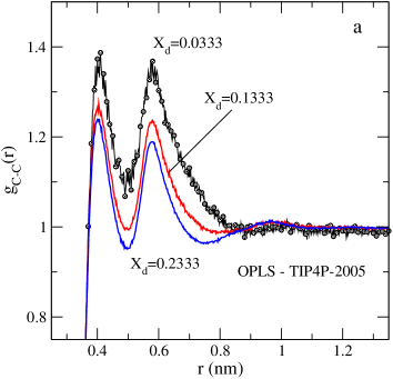
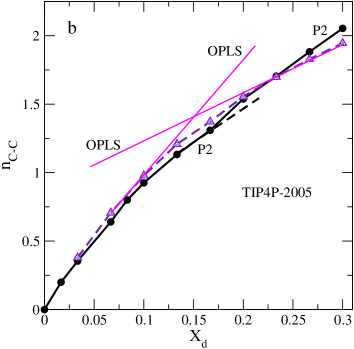
Figure 8: (Colour online) Panel a: evolution of the pair distribution function of methyl groups for the OPLS-TIP4P-2005 model at different compositions $X_{d}$. Panel b: coordination number of a single methyl group on composition changes of water-DMSO mixtures from the OPLS-TIP4P-2005 and P2-TIP4P-2005 models.

3.5 Self-diffusion coefficients of DMSO and water molecules

We proceed now to the description of the behavior of the self-diffusion coefficients of species, $D_{i}$ ($i=w$, DMSO), upon changing composition of the mixture. In figure 9 we show the results obtained via the Einstein relation,

$$D_{i}=\frac{1}{6}\lim_{t\rightarrow\infty}\frac{\mathrm{d}}{\mathrm{d}t}|{\bf r}_{i}(\tau+t)-{\bf r}_{i}(\tau)|^{2},$$ (3.4)

where $\tau$ denotes the time origin. Default settings of GROMACS were used for the separation of the time origins and for the fitting interval. The experimental data were taken from references [60, 61]. According to the experiments, the self-diffusion coefficient of water species decreases in magnitude starting from pure water value (at $X_{d}$ = 0) and reaches minimum at $X_{d}\approx 0.3$. Next, for higher $X_{d}$, $D_{w}$ does not change much, but a certain pecuiliarity is seen in the interval between 60% and 80%. Apparently, the behavior of $D_{i}(X_{d})$ is determined by the evolution of density of the mixture and by the hydrogen bonding between species. Theoretical predictions for $D_{w}$ lead to a bit inaccurate, but still satisfactory agreement with experimental trends for water-rich mixtures. The OPLS-TIP4P-2005 model looks the best, because it underestimates the density in the entire composition interval starting from water-rich and ending up at DMSO-rich mixtures, cf. figure 1. This model yields a good value for $D_{w}$ close to $X_{d}=1$, as well. Both, the P1-TIP4P-2005 and P2-TIP4P-2005 model yield qualitatively correct trends but essentially underestimate $D_{w}$ in a wide interval of compositions. Besides two factors mentioned just above, we can attribute such low values for $D_{w}$ to the pronounced inaccuracy of description of the energetic factors of mixing of species in the framework of these two models, cf. figure 4 b. Better performance of the OPLS-TIP4P-2005 model for the excess mixing enthalpy apparently contributes to better description of $D_{w}$.

According to the experimental data by Packer and Tomlinson [60], the self-diffusion coefficient of DMSO species has a minimum at $X_{d}\approx$ 0.7. Besides, there is a peculiarity of $D_{\rm{DMSO}}$ in the interval of compositions corresponding to water-rich mixtures. The model of the present study yields satisfactory predictions for $D_{\rm{DMSO}}$ close to $X_{d}\approx 0$. Each of the models in question exhibits a weakly pronounced peculiarity around $X_{d}\approx 0.1$. However, this peculiarity is much weaker compared to what one observes from experimental points. On the other hand, close to $X_{d}\approx 1$, the P1-TIP4P-2005 model describes $D_{\rm{DMSO}}$ pretty well. However, the minimum predicted by the models occurs at intermediate compositions around 0.5, rather than at 0.7 from the experimental points.

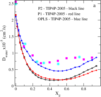
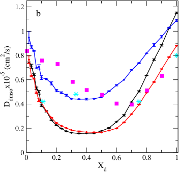
Figure 9: (Colour online) Panels a and b: composition dependence of the self-diffusion coefficient of water-DMSO mixtures at 298.15 K for different combinations of DMSO and water models. Experimental data are from reference [60] (squares) and from reference [61] (stars).

To summarize, the models used in simulation perform better at “wings”, i.e., close to $X_{d}\approx 0$ and $X_{d}\approx 1$, rather than at intermediate compositions. Still, the dynamic aspects of mixing are apparently better described for water-rich mixtures. We have not performed a detailed investigation of the self-diffusion coefficient of species for DMSO models combined with TIP4P/$\varepsilon$ model. It is known that the diffusion coefficient of pure water in the framework of TIP4P-2005 and TIP4P/$\varepsilon$ model is very similar [45]. Thus, we do not expect to obtain an improvement of the observed trends by changes of the water models of this type.

The missing elements worth to explore are various. Namely, it is necessary to confirm the present results by using alternative calculations of the self-diffusion coefficients via the velocity auto-correlation functions. In addition, one should attempt to calculate the relaxation times and possibly the power spectra, similarly to e.g., [62], because of the availability of experimental data. It would provide ampler insights into the adequacy of the force fields.

3.6 Static dielectric constant of water-DMSO mixtures

Now, proceed to the results for the static dielectric constant. It is one of the most difficult properties to deal with. Recently, we explored the dielectric constant for water-DMSO mixtures by using the SPC-E water model [33]. Therefore, the present discussion will be brief and solely novel findings will be underlined.

The long-range, asymptotic behavior of correlations between the molecules possessing a dipole moment is described by the dielectric constant, $\varepsilon$, which is calculated from the time-average of the fluctuations of the total dipole moment of the system [63] as follows,

$$\varepsilon=1+\frac{4\piup}{3k_{\rm{B}}TV}\left(\langle\bf M^{2}\rangle-\langle\bf M\rangle^{2}\right),$$ (3.5)

where $k_{\rm{B}}$ is the Boltzmann constant and $V$ is the simulation cell volume. In this work we took care that each of the runs is of sufficient time extension (more than 100 ns in all cases), in order to obtain reasonable statistics. The final value was recorded. In contrast to reference [33], the averaging over blocks was not performed. Besides the stability of the dielectric constant value along the run, we verified the temporal behavior of the average total polarization of the system to ensure that each of the components ($x$, $y$ and $z$) is close to zero. Evidently, the number of molecules, type of thermostat and barostat, precision of the long-range interactions summation contribute into the accuracy of the evaluation of the dielectric constant.

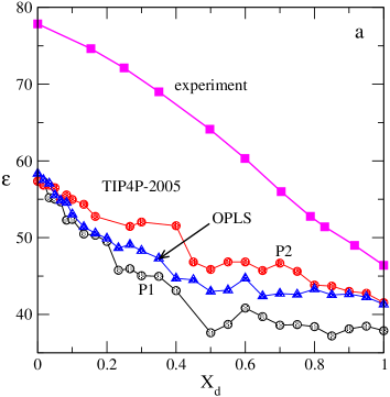
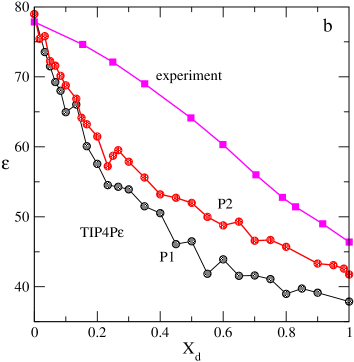
Figure 10: (Colour online) Panels a and b: composition dependence of the static dielectric constant of water-DMSO mixtures at 298.15 K for different combinations of DMSO and water models. Experimental data are from reference [64].

The experimental data are taken from reference [64]. The dielectric constant decreases from a high value for water to a much lower value for pure DMSO. According to the experiment, the inclination of the curve for $\varepsilon(X_{d})$ changes around $X_{d}\approx 0.2$. Moreover, the dielectric constant is almost linear for $X_{d}>0.8$. It is known that the TIP4P-2005 does not provide a reasonable description of the dielectric constant for pure water. Thus, if one changes the DMSO model, the results do not improve on the water-rich side of the composition, panel a of figure 10. On the DMSO-rich side, the OPLS and P2 models, if combined with TIP4P-2005 water model, yield not very bad values for $\varepsilon$. However, general trends of decay of $\varepsilon$ with increasing $X_{d}$ are not satisfactory. In spite of long time of simulations, the values for $\varepsilon$ strongly fluctuate along $X_{d}$ axis, such that it is impossible to capture any confiable peculiarities. Substantial improvement of the results is reached, if one substitutes TIP4P-2005 water model by the TIP4P/$\varepsilon$ model. Then, the values for dielectric constant essentially improve for water-rich mixtures. Moreover, the simulation data fluctuate less upon changing the composition $X_{d}$. Two regions of behavior can be identified. Namely, the simulation data predict a fast decay of $\varepsilon$ for water-rich mixtures and a slower decay in the opposite interval of compositions, say at $X_{d}>0.3$. The experimental points, by contrast, show a slower decay for a water-rich mixture and a slightly weaker decay at higher values of $X_{d}$. After long runs (150 ns), we obtained with confidence a peculiarity in the values of $\varepsilon$ in the interval of $X_{d}$ between 0.2 and 0.3. It is similar by shape to the behavior of mean square deviation of total dipole moment on composition plotted in figure 3 of reference [22] at $X_{d}$ between 0.1 and 0.15 with another force field. These trends, however, result from the modelling rather than from the experimental observations. In view of the present findings, the interpretation of data in terms of structural phase transition in laboratory systems seems to be questionable.

Apparently, the inaccuracy of the description of energetic trends of mixing the water and DMSO species in the framework of P1 and P2 DMSO models leads to unsatisfactory dependence of the dielectric constant on $X_{d}$. In qualitative terms, the conclusion is similar to what was mentioned above concerning the self-diffusion coefficients of species. However, it is worth to complement the calculations of the dielectric constant by the exploration of the behavior of the Kirkwood factor. There is room for intent improvement of the data. One can consider larger systems, exclude the fluctuations of pressure by switching to the canonical, NVT, ensemble, take larger values for cut-off distance. Application of these technical issues does not guarantee better results. Seemingly, present non-polarizable DMSO models with the present schemes of taking into account the long-range electrostatic interactions are incapable of reproducing the experimental data. Definitely, the situation improves if one applies even simple polarizable DMSO model, see e.g. [31]. Then, one would expect that the combination of the TIP4P/$\varepsilon$ water with even simplified polarizable DMSO model would be profitable. These issues guarantee future studies.

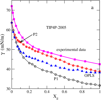
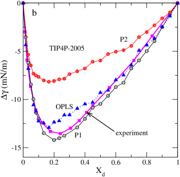
Figure 11: (Colour online) Composition dependence of the surface tension (panel a) and of the excess surface tension (panel b) for different combinations of DMSO and water models. Experimental data are taken from reference [66].

3.7 Surface tension of water-DMSO mixtures on composition

Our final remarks concern the behavior of the surface tension of water-DMSO mixtures. The surface tension calculations at each composition were performed by taking the final configuration of particles from the isobaric run. Next, the box edge along $z$-axis was extended by a factor of 3, generating a rectangular box with a liquid slab and two liquid-mixture-vacuum interfaces in the $x-y$ plane, in close similarity to the procedure applied in [65]. The total number of molecules is sufficient to yield sufficiently big area of the $x-y$ face of the liquid slab. The elongation of the liquid slab along $z$-axis is satisfactory as well. The executable file was modified by deleting a fixed pressure condition preserving the V-rescale thermostatting with the same parameters as in the NPT runs. Other corrections were not employed. The values for the surface tension, $\gamma$, follow from the combination of the time averages for the components of the pressure tensor,

$$\gamma=\frac{1}{2}L_{z}\left\langle{\left[P_{zz}-\frac{1}{2}\left(P_{xx}+P_{yy}\right)\right]}\right\rangle,$$ (3.6)

where $P_{ij}$ are the components of the pressure tensor along $i,j$ axes, and $\langle...\rangle$ denotes the time average. We performed five runs at a constant volume, each piece of 10 ns, and obtained the result for $\gamma$ by taking the block average. The experimental results were taken from reference [66]. The data show that the surface tension rapidly decreases from the pure water value at $X_{d}=0$ till $X_{d}\approx 0.25$. Next, at higher values of $X_{d}$, the values for $\gamma$ decrease more slowly, the curve behaves almost linearly in that interval of compositions, panel a of figure 11. The excess surface tension from experiment exhibits minimum at $X_{d}\approx 0.25$. All the models in question behave similarly for water-rich mixtures. The decay of $\gamma$ is better reproduced by P1-TIP4P-2005 and OPLS-TIP4P-2005 models, rather than by P2-TIP4P-2005 model. The absolute values for $\gamma$ are underestimated, but can be improved by including the long-range corrections.

Concerning the behavior of $\gamma$ for DMSO-rich mixtures, one should note that the P2-TIP4P-2005 model leads to the results most close to the experimental data. However, the excess surface tension is underestimated by this model intermediate compositions. On the other hand, the P1-TIP4P-2005 and OPLS-TIP4P-2005 reproduce the excess surface tension rather well in the entire interval of compositions, panel b of figure 11. The shape of the surface tension on $X_{d}$ is quite well reproduced by these two models, just the absolute values of $\gamma$ are underestimated. Thus, a reasonable description of $\gamma$ and its excess simultaneously by the models of this study restricts to water-rich mixtures. Still, it seems that a better agreement with experimental data may result from the changes of fine details of simulation procedure as documented in reference [67].

4 Summary and conclusions

Recently we studied the properties of water-DMSO liquid mixtures in the entire composition interval by molecular dynamics computer simulations of the DMSO models combined with the SPC-E water model [33]. In the present work, we explore the same systems with the same methodology but using the non-polarizable, P1, P2 and OPLS united atom DMSO models in conjunction with the TIP4P-2005 and TIP4P/$\varepsilon$ water models. Concerning the DMSO models, we observed that the flexibility of angles, keeping the bond constrained, requires to include the dihedral angle as recommended in reference [42]. The systems in question are studied at room temperature, 298.15 K and atmospheric pressure, 0.1 MPa, as previously.

A set of novel findings was obtained and discussed in every detail. Namely, in the present work we obtained the excess partial molar volumes and apparent molar volumes. Analyses of these properties permitted us to capture an anomalous behavior observed at low DMSO molar fraction in agreement with experimental results. Besides, the excess partial molar enthalpy of each species was obtained and compared with experimental findings. Particular emphasis was put on the elucidation of the behavior of various radial distribution functions in water-rich mixtures. The coordination numbers and the fractions of molecules participating in hydrogen bonds were involved in the interpretation of the microscopic structure. The self-diffusion coefficients of species were obtained and compared with experimental data. Next, the static dielectric constant was calculated and compared with experimental results. Our final focus was on elucidating the behavior of the surface tension on the composition of water-DMSO mixtures and of the excess surface tension. Their trends were compared with experimental data. A very detailed validation of the predictions of the properties resulting from a set of models for water-DMSO solutions permit to make conclusions w.r.t. their applicability.

Among the variety of our results, solely the discussion of changes of the microscopic structure lacks comparison with experiments. In order to do that, one needs to have data concerning the total and desirably the partial structure factors in the entire composition interval. Then, it would be possible to perform the analyses similar to what was done in this laboratory for water-methanol mixtures [62]. We are not aware of such type of results for water-DMSO mixtures at present. This part of study of water-DMSO mixtures might benefit from the reverse Monte Carlo modelling in order to elucidate fine features of the hydrogen bonded network, see e.g., [56]. An illuminating finding about the existence and lifetime of frequently discussed complexes or associates may be expected.

According to our findings, one can distinguish two types of properties. Namely, for one type, the role of fluctuations is less important. Evidently, at a fixed pressure the systems’ volume fluctuates, but density as an average over a set of computer simulation runs is well defined. The density dependence on composition compares well with experiment. Consequently, one is able to describe well the excess partial molar volumes and apparent molar volumes and definitely prove the existence of an anomalous behavior for water-rich water-DMSO mixtures. Previously, this kind of behavior was obtained and discussed for water-methanol mixtures [68, 69].

On the other hand, under the same conditions to obtain the isothermal compressibility, for example, requires time average of fluctuations. Consequently, this property is more difficult to obtain. Similarly, a disappointing situation is observed in the calculations of the static dielectric constant. It results from the time evolution of the total dipole moment fluctuations. If $\varepsilon$ is calculated from the NPT runs, the volume fluctuations contribute to the inaccuracy of the results. In addition, at a constant density, the values for $\varepsilon$ are affected by the choice of the number of particles in the simulation box, by the assumed cut-off of the interactions and by the scheme of summation of long-range interaction effects.

One should have these difficulties in mind while interpreting the changes of various properties on composition. Specifically, we observed that peculiarities of the behavior of different descriptors hardly permit to interpret them as discontinuous structural transitions in laboratory systems, see e.g., figures 3 and 5 of reference [22] and figures 8 and 9 of reference [20], unless a precise description of the underlying properties in terms of microscopic structure and/or the static dielectric constant is obtained by computer simulations.

To summarize, we would like to mention that each of the explored models was designed, or say parametrized, using a restricted number of different criteria at certain thermodynamic conditions. Thus, it is difficult to expect that modelling can be successful in a wide range of temperature and pressure. Similarly, we observed “non-universal” performance of the models along the composition axes. It appears that the P2-TIP4P-2005 model provides a reasonable description of a wide set of properties for water-rich mixtures, except the static dielectric constant. However, this behavior can be mitigated by using the P2 - TIP4P/$\varepsilon$ model. In addition, we would like to note that the P1-TIP4P-2005 model is better than the P2-TIP4P-2005 model for some properties of DMSO-rich mixtures and describes the surface tension and the excess surface tension reasonably well. Hence, one should choose the working model dependent on how concentrated DMSO solution is necessary to deal with, besides the pressure and temperature values of the given setup. The OPLS-TIP4P-2005 model is successful solely for a few properties. Hence, possible modifications of the parameters and combination rules should be attempted.

Finally, we would like to enlist a few missing elements to extend our knowledge of the properties of water-DMSO mixtures. It would be profitable to explore various velocity auto-correlation functions to enhance the understanding of dynamic properties, as well as to investigate Kirkwood factors and possibly the frequency dependent dielectric constant to understand the dielectric properties better. Another missing issue is to explore the cooperativity of hydrogen bond network in terms of certain complex elements, see e.g., [59], and hydrogen bonds life times.

Ukrainian 0

Ùå ðàç ïðî êîíöåíòðàöiéíi çàëåæíîñòi âëàñòèâîñòåé ðiäêèõ ñóìiøåé âîäà-äèìåòèëñóëüôîêñèä. Ìîäåëþâàííÿ ìåòîäîì ìîëåêóëÿðíî¿ äèíàìiêè. M. Àãiëàð${}^{\textsf{\footnotesize{\mbox{?}}}}$, Å. Äîìiíãåñ${}^{\textsf{\footnotesize{\mbox{?}}}}$, O. Ïiçiî${}^{\textsf{\footnotesize{\mbox{?}}}}$

             
${}^{\textsf{\footnotesize 1}}$ Iíñòèòóò õiìi¿, Íàöiîíàëüíèé àâòîíîìíèé óíiâåðñèòåò Ìåõiêî, Circuito Exterior, 04510, Ìåõiêî, Ìåêñèêà ${}^{\textsf{\footnotesize 2}}$ Iíñòèòóò äîñëiäæåííÿ ìàòåðiàëiâ, Íàöiîíàëüíèé àâòîíîìíèé óíiâåðñèòåò Ìåõiêî, Circuito Exterior, 04510, Ìåõiêî, Ìåêñèêà

References

- [1] Jacob S. W., Rosenbaum E. E., Wood D. C. (Eds.), Dimethyl Sulfoxide, Marcel Dekker, New York, 1971.
-
[2]
Martin D., Weise A., Nicklas H. J., Angew. Chem. Int. Ed. Engl., 1967, 6, 318,
doi:10.1002/anie.196703181. - [3] Martin D., Hauthal H. G., Dimethyl Sulfoxide, Wiley, New York, 1975.
- [4] McGann L. E., Walterson M. L., Cryobiology, 1987, 24, 11, doi:10.1016/0011-2240(87)90003-4.
- [5] Murthy S. S. N., J. Phys. Chem., 1997, 101, 6043, doi:10.1021/jp970451e.
-
[6]
Ehrlich L. E., Feig J. S. G., Schiffres S. N., Malen J. A., Rabin Y., PLoS ONE, 2015, 10, e0125862,
doi:10.1371/journal.pone.0125862. - [7] Wiewiór P. P., Shirota H., Castner E. W., J. Chem. Phys., 2002, 116, 4643, doi:10.1063/1.1449864.
- [8] Rao B. G., Singh U. C., J. Am. Chem. Soc., 1990, 112, 3803, doi:10.1021/ja00166a014.
- [9] Vaisman I. I., Berkowitz M. L., J. Am. Chem. Soc., 1992, 114, 7889, doi:10.1021/ja00046a038.
- [10] Luzar A., Chandler D., J. Chem. Phys., 1993, 98, 8160, doi:10.1063/1.464521.
- [11] Liu H., Mueller-Plathe F., van Gunsteren W. F., J. Am. Chem. Soc., 1995, 117, 4363, doi:10.1021/ja00120a018.
- [12] Onthong U., Megyes T., Bakó I., Radnai T., Grósz T., Hermansson K., Probst M., Phys. Chem. Chem. Phys., 2004, 6, 2136, doi:10.1039/B311027C.
- [13] Idrissi A., Marekha B., Barj M., Jedlovszky P., J. Phys. Chem. B, 2014, 118, 8724, doi:10.1021/jp503352f.
- [14] Chalaris M., Samios J., J. Mol. Liq., 2002, 98–99, 401, doi:10.1016/S0167-7322(01)00344-0.
-
[15]
Geerke D. P., Oostenbrink C., van der Vegt N. F. A.,
van Gunsteren W. F., J. Phys. Chem. B, 2004, 108, 1436,
doi:10.1021/jp035034i. - [16] Borin I. A., Skaf M. S., J. Chem. Phys., 1999, 110, 6412, doi:10.1063/1.478544.
- [17] Skaf M. S., J. Phys. Chem. A, 1999, 103, 10719, doi:10.1021/jp992247s.
- [18] Vishnyakov A., Lyubartsev A. P., Laaksonen A., J. Phys. Chem. A, 2001, 105, 1702, doi:10.1021/jp0007336.
-
[19]
Mancera R. L., Chalaris M., Refson K., Samios J., Phys. Chem. Chem. Phys., 2004, 6, 94,
doi:10.1039/B308989D. - [20] Banerjee S., Roy S., Bagchi B., J. Phys. Chem. B, 2010, 114, 12875, doi:10.1021/jp1045645.
- [21] Pojják K., Darvas M., Horvai G., Jedlovszky P., J. Phys. Chem. C, 2010, 114, 12207, doi:10.1021/jp101442m.
- [22] Roy S., Banerjee S., Biyani N., Jana B., Bagchi B., J. Phys. Chem. B, 2011, 115, 685, doi:10.1021/jp109622h.
- [23] Perera A., Mazighi R., J. Chem. Phys., 2015, 143, 154502, doi:10.1063/1.4933204.
-
[24]
Idrissi A., Marekha B., Kiselev M., Jedlovszky P.,
Phys. Chem. Chem. Phys., 2015, 17, 3470,
doi:10.1039/C4CP04839C. - [25] Strader M. L., Feller S. E., J. Phys. Chem. A, 2002, 106, 1074, doi:10.1021/jp013658n.
- [26] Zhang N., Li W., Chen C., Zuo J., Comput. Theor. Chem., 2013, 1017, 126, doi:10.1016/j.comptc.2013.05.018.
- [27] Fox T., Kollman P. A., J. Phys. Chem. B, 1998, 102, 8070, doi:10.1021/jp9717655.
- [28] Benjamin I., J. Chem. Phys., 1999, 110, 8070, doi:10.1063/1.478708.
- [29] Senapati S., J. Chem. Phys., 2002, 117, 1812, doi:10.1063/1.1489898.
- [30] Zhang Q., Zhang X., Zhao D. X., J. Mol. Liq., 2009, 145, 67, doi:10.1016/j.molliq.2009.01.003.
- [31] Bachmann S. J., van Gunsteren W. F., J. Phys. Chem. B, 2014, 118, 10175, doi:10.1021/jp5035695.
-
[32]
Bordat P., Sacristan J., Reith D., Girard S., Glättli A., Müller-Plathe F., Chem. Phys. Lett., 2003, 374, 201,
doi:10.1016/S0009-2614(03)00550-5. - [33] Gujt J., Vargas E. C., Pusztai L., Pizio O., J. Mol. Liq., 2017, 228, 71, doi:10.1016/j.molliq.2016.09.024.
- [34] Roy S., Bagchi B., J. Chem. Phys., 2013, 139, 034308, doi:10.1063/1.4813417.
- [35] Martins L. R., Skaf M. S., Chem. Phys. Lett., 2003, 370, 683, doi:10.1016/S0009-2614(03)00159-3.
- [36] Laria D., Skaf M. S., J. Chem. Phys., 1999, 111, 300, doi:10.1063/1.479290.
- [37] Martins L. R., Tamashiro A., Laria D., Skaf M. S., J. Chem. Phys., 2003, 118, 5955, doi:10.1063/1.1556296.
- [38] Wong D. B., Sokolowsky K. P., El-Barghouthi M. I., Fenn E. E., Giammanco C. H., Sturlaugson A. L., Fayer M. D., J. Phys. Chem. B, 2012, 116, 5479, doi:10.1021/jp301967e.
- [39] Roy D., Kovalenko A., J. Comput.-Aided Mol. Des., 2019, 33 905, doi:10.1007/s10822-019-00238-4.
- [40] Chalaris M., Marinakis S., Dellis D., Fluid Phase Equilib., 2008, 267, 47, doi:10.1016/j.fluid.2008.02.019.
- [41] Jorgensen W. L., Maxwell D. S., Tirado-Rives J., J. Am. Chem. Soc., 1996, 118, 11225, doi:10.1021/ja9621760.
-
[42]
Oostenbrink C., Villa A., Mark A. E., van Gunsteren W. F.,
J. Comput. Chem., 2004, 25, 1656,
doi:10.1002/jcc.20090. - [43] Skaf M., J. Chem. Phys., 1997, 107, 7996, doi:10.1063/1.475062.
- [44] Abascal J. L. F., Vega C., J. Chem. Phys., 2005, 123, 234505, doi:10.1063/1.2121687.
- [45] Fuentes-Azcatl R., Alejandre J., J. Phys. Chem. B, 2014, 118, 1263, doi:10.1021/jp410865y.
- [46] van der Spoel D., Lindahl E., Hess B., Groenhof G., Mark A. E., Berendsen H. J. C., J. Comput. Chem., 2005, 26, 1701, doi:10.1002/jcc.20291.
- [47] Egorov G. I., Makarov D. M., Russ. J. Phys. Chem. A, 2009, 83, 693, doi:10.1134/S003602440905001X.
- [48] Hernandez-Perni G., Leuenberger H., Eur. J. Pharm. Biopharm., 2005, 61, 201, doi:10.1016/j.ejpb.2005.05.008.
-
[49]
Tôrres R. B., Marchiore A. C. M., Volpe P. L. O., J. Chem. Thermodyn., 2006, 38, 526,
doi:10.1016/j.jct.2005.07.012. -
[50]
Grande M. C., Juliá J. Á., García M., Marschoff C. M.,
J. Chem. Thermodyn., 2007, 39, 1049,
doi:10.1016/j.jct.2006.12.012. -
[51]
Rodnikova M. N., Zakharova Yu. A., Solonina I. A., Sirotkin D. A., Russ.
J. Phys. Chem. A, 2012, 86, 892,
doi:10.1134/S0036024412050317. - [52] Clever H. L., Pigott S. P., J. Chem. Thermodyn., 1971, 3, 221, doi:10.1016/S0021-9614(71)80106-4.
- [53] Rallo F., Rodante F., Silvestroni P., Thermochim. Acta, 1970, 1, 311, doi:10.1016/0040-6031(70)80013-2.
- [54] Lai J. T. W., Lau F. W., Robb D., Westh P., Nielsen G., Trandum C., Hvidt A., Koga Y., J. Solution Chem., 1995, 24, 89, doi:10.1007/BF00973051.
- [55] Cowie J. M. G., Toporowski P. M., Can. J. Chem., 1961, 39, 2240, doi:10.1139/v61-296.
- [56] Pusztai L., Pizio O., Sokolowski S., J. Chem. Phys., 2008, 129, 184103, doi:10.1063/1.2976578.
-
[57]
Galicia-Andrés E., Pusztai L., Temleitner L., Pizio O.,
J. Mol. Liq., 2015, 209, 586,
doi:10.1016/j.molliq.2015.06.045. -
[58]
Bakó I., Megyes T., Bálint S., Grósz T., Chihaia V., Phys. Chem. Chem. Phys.,
2008, 10, 5004,
doi:10.1039/B808326F. - [59] Bakó I., Pusztai L., Temleitner L., Sci. Rep., 2017, 7, 1073, doi:10.1038/s41598-017-01095-7.
- [60] Packer K. J., Tomlinson D. J., Trans. Faraday Soc., 1971, 67, 1302, doi:10.1039/TF9716701302.
-
[61]
Bordallo H. N., Herwig K. W., Luther B. M., Levinger N. E., J. Chem. Phys., 2004, 121, 12457,
doi:10.1063/1.1823391. -
[62]
Galicia-Andrés E., Dominguez H., Pusztai L., Pizio O.,
J. Mol. Liq., 2015, 212, 70,
doi:10.1016/j.molliq.2015.08.061. - [63] Neumann M., Mol. Phys., 1983, 50, 841, doi:10.1080/00268978300102721.
- [64] Płowaś I., Świergiel J., Jadżyn J., J. Chem. Eng. Data, 2013, 58, 1741, doi:10.1021/je400149j.
- [65] Fischer N. M., van Maaren P. J., Ditz J. C., Yildirim A., van der Spoel D., J. Chem. Theory Comput., 2015, 11, 2938, doi:10.1021/acs.jctc.5b00190.
-
[66]
Golmaghani-Ebrahimi E., Bagheri A., Fazli M., J. Chem. Thermodyn., 2020, 146,
106105,
doi:10.1016/j.jct.2020.106105. - [67] Zubillaga R. A., Labastida A., Cruz B., Martínez J. C., Sánchez E., Alejandre J., J. Chem. Theory Comput., 2013, 9, 1611, doi:10.1021/ct300976t.
- [68] Cruz Sanchez M., Aguilar M., Pizio O., Condens. Matter Phys., 2020, 23, 34601, doi:10.5488/CMP.23.34601.
-
[69]
Chechko V. E., Gotsulsky V. Ya., Malomuzh M. P., Condens. Matter Phys., 2013,
16, 23006,
doi:10.5488/CMP.16.23006.
Ukrainian \adddialect\l@ukrainian0 \l@ukrainian