Learning Algorithm Generalization Error Bounds via Auxiliary Distributions

Abstract

Generalization error boundaries are essential for comprehending how well machine learning models work. In this work, we suggest a creative method, i.e., the Auxiliary Distribution Method, that derives new upper bounds on generalization errors that are appropriate for supervised learning scenarios. We show that our general upper bounds can be specialized under some conditions to new bounds involving the generalized $\alpha$-Jensen-Shannon, $\alpha$-Rényi ($0<\alpha<1$) information between random variable modeling the set of training samples and another random variable modeling the set of hypotheses. Our upper bounds based on generalized $\alpha$-Jensen-Shannon information are also finite. Additionally, we demonstrate how our auxiliary distribution method can be used to derive the upper bounds on generalization error under the distribution mismatch scenario in supervised learning algorithms, where the distributional mismatch is modeled as $\alpha$-Jensen-Shannon or $\alpha$-Rényi ($0<\alpha<1$) between the distribution of test and training data samples. We also outline the circumstances in which our proposed upper bounds might be tighter than other earlier upper bounds.

I Introduction

Numerous methods have been proposed in order to describe the generalization error of learning algorithms. These include VC-based bounds [2], algorithmic stability-based bounds [3], algorithmic robustness-based bounds [4], PAC-Bayesian bounds [5]. Nevertheless, for a number of reasons, many of these generalisation error bounds are unable to describe how different machine-learning techniques can generalise: some of the bounds depend only on the hypothesis class and not on the learning algorithm; existing bounds do not easily exploit dependencies between different hypotheses; or do not exploit dependencies between the learning algorithm input and output.

More recently, methods that make use of information-theoretic tools have also been developed to describe the generalisation of learning techniques. Such methods frequently incorporate the many components related to the learning problem by expressing the generalisation error in terms of certain information measurements between the learning algorithm input (the training dataset) and output (the hypothesis). In particular, building upon pioneering work by Russo and Zou [6], Xu and Raginsky [7] have derived generalization error bounds involving the mutual information between the training set and the hypothesis. Bu et al. [8] have derived tighter generalization error bounds involving the mutual information between each individual sample in the training set and the hypothesis. Meanwhile, bounds using chaining mutual information have been proposed in [9, 10]. Other authors have also constructed information-theoretic based generalization error bounds based on other information measures such as $\alpha$-Rényi divergence for $\alpha>1$, $f$-divergence, and maximal leakage [11]. In [12], an upper bound based on $\alpha$-Rényi divergence for $0<\alpha<1$ is derived by using the variational representation of $\alpha$-Rényi divergence. Bounds based on the Wasserstein distance between the training sample data and the output of a randomized learning algorithm [13], [14] and Wasserstein distance between distributions of an individual sample data and the output of the learning algorithm are proposed in [15], and tighter upper bounds via convexity of Wasserstein distance are proposed in [16]. Upper bounds based on conditional mutual information and individual sample conditional mutual information are proposed in [17] and [18], respectively. The combination of conditioning and processing techniques can provide tighter generalization error upper bounds [19, 20]. An exact characterization of the generalization error for the Gibbs algorithm in terms of symmetrized KL information is provided in [21], and is extended for transfer learning scenario in [22].

Generalization error bounds have also been developed to address scenarios where the training data distribution differs from the test data distribution, known as Distribution Mismatch. This scenario – which also links to out-of-distribution generalization – has attract various contributions in recent years such as [23, 24, 25]. In particular, Masiha et al. [26] provides information-theoretic generalization error upper bounds in the presence of training/test data distribution mismatch, using rate-distortion theory. The Covariate-shift as a distribution mismatch scenario in semi-supervised learning is studied in [27].

In this work, we propose an auxiliary distribution method (ADM) to characterize the generalization error upper bound of supervised learning algorithms in terms of novel information measures. Our new bounds offer two advantages over existing ones: (1) Some of our bounds – such as the generalized $\alpha$-Jensen-Shannon information ones – are always finite, whereas conventional mutual information ones (e.g., [7]) may not be; (2) In contrast to mutual information-based bounds, our bounds—such as the $\alpha$-Rényi information for $0<\alpha<1$—are finite for some deterministic supervised learning algorithms; (3) We also apply ADM to provide an upper bound on generalization error of supervised learning algorithms under distribution mismatch between test and training data distributions. The distribution mismatch between test and training dataset is measured by some novel divergences between the distributions of test and training data samples.

In summary, our main contributions are as follows:

1. We suggest a novel method, i.e., ADM, that uses auxiliary distributions over the spaces of the hypothesis and data sample to obtain upper bounds on the generalization error.

2. Using this approach that one can derive new generalization error bounds expressed via generalized $\alpha$-Jensen-Shannon divergence which is known to be finite.

3. Using ADM, we offer an upper bound based on $\alpha$-Rényi divergence for $0<\alpha<1$ with the same decay rate as the mutual information-based upper bound. Furthermore, in contrast to the mutual information-based bounds, the $\alpha$-Rényi divergence bounds for $0<\alpha<1$ are finite when the hypothesis (output of the learning algorithm) is a deterministic function of at least one data sample.

4. Using ADM, we also provide generalization error upper bound under training and test data distribution mismatch. It turns out that training and test distribtion mismatch is captured in our upper bounds via generalized $\alpha$-Jensen-Shannon or $\alpha$-Rényi divergences.

It is noteworthy to add that, although the generalized $\alpha$-Jensen-Shannon measure does not appear to have been used to characterize the generalization ability of learning algorithms, these information-theoretic quantities as well as $\alpha$-Rényi measure for $0<\alpha<1$, have been employed to study some machine learning problems, including the use of

• generalized $\alpha$-Jensen-Shannon as a loss function under label noise scenario [28], and Jensen-Shannon divergence (generalized $\alpha$-Jensen-Shannon divergence for $\alpha=1/2$) in adversarial learning [29] and active learning [30].

• $\alpha$-Rényi divergence in feature extraction  [31] and image segmentation based on clustering [32].

II Problem Formulation

II-A Framework of Statistical Learning

We analyse a standard supervised learning setting where we wish to learn a hypothesis given a set of input-output examples that can then be used to predict a new output given a new input.

In particular, in order to formalize this setting, we model the input data (also known as features) using a random variable $X\in\mathcal{X}$ where $\mathcal{X}$ is the input space, and we model the output data (also known as predictors or labels) using a random variable $Y\in\mathcal{Y}$ where $\mathcal{Y}$ is the output space. We also model input-output data pairs using a random variable $Z=(X,Y)\in\mathcal{Z}=\mathcal{X}\times\mathcal{Y}$ where $Z$ is drawn from $\mathcal{Z}$ per some unknown distribution $\mu$. We also let $S=\{Z_{i}=(X_{i},Y_{i})_{i=1}^{n}\}$ be a training set consisting of $n$ input-output data points drawn i.i.d. from $\mathcal{Z}$ according to $\mathcal{\mu}$.

We denote hypotheses by a random variable $W\in\mathcal{W}$ ($W:\mathcal{X}\rightarrow\mathcal{Y}$) where $\mathcal{W}$ is a hypothesis class. Finally, we represent a learning algorithm via a Markov kernel that maps a given training set $S$ onto hypothesis $W$ defined on the hypothesis class $\mathcal{W}$ according to the probability law $P_{W|S}$.

We introduce a (non-negative) loss function $\ell:\mathcal{W}\times\mathcal{Z}\rightarrow\mathbb{R}^{+}$ that measures how well a hypothesis predicts an output given an input. We can now define the population risk and the empirical risk associated with a given hypothesis as follows:

$$L_{P}(w,\mu)\triangleq\int_{\mathcal{Z}}\ell(w,z)d\mu(z),$$ (1)

$$L_{E}(w,s)\triangleq\frac{1}{n}\sum_{i=1}^{n}\ell(w,z_{i}),$$ (2)

respectively. We can also define the (expected) generalization error as follows:

$$\overline{\operatorname*{gen}}(P_{W|S},\mu) \triangleq\mathbb{E}_{P_{W,S}}[\text{gen}(W,S,\mu)],$$ (3)

where $\text{gen}(w,s,\mu)\triangleq L_{P}(w,\mu)-L_{E}(w,s)$. This (expected) generalization error quantifies by how much the population risk deviates from the empirical risk. This quantity cannot be computed directly because $\mu$ is unknown, but it can often be (upper) bounded, thereby providing a means to gauge various learning algorithms’ performance.

We also analyse a supervised learning scenario under distribution mismatch, where training and test data are drawn from different distributions ($\mu$ and $\mu^{\prime}$, respectively). In particular, we define the population risk based on test distribution $\mu^{\prime}$ as follows:

$$L_{P}(w,\mu^{\prime})\triangleq\int_{\mathcal{Z}}\ell(w,z)d\mu^{\prime}(z).$$ (4)

We define the mismatched(expected) generalization error as follows:

$$\overline{\operatorname*{gen}}(P_{W|S},\mu,\mu^{\prime}) \triangleq\mathbb{E}_{P_{W,S}}[\text{gen}(W,S,\mu,\mu^{\prime})],$$ (5)

where $\text{gen}(w,s,\mu,\mu^{\prime})\triangleq L_{P}(w,\mu^{\prime})-L_{E}(w,s)$.

Our goal in the sequel will be to derive (upper) bounds on the generalization errors (3) and the mismatched(expected) generalization error (5) expressed via various information-theoretic measures.

II-B Auxiliary Distribution Method

We now describe our main method to derive the generalization error upper bounds, i.e., the ADM. Consider $P$ and $Q$ as two distributions defined on a measurable space $\mathcal{X}$ and let $f:\mathcal{X}\to\mathbb{R}$ be a measurable function. Assume that we can use an asymmetric information measure $T(P\|Q)$ between $P$ and $Q$ to construct the following upper bound:

$$\left|\mathbb{E}_{P}[f(X)]-\mathbb{E}_{Q}[f(X)]\right|\leq F(T(P\|Q)),$$ (6)

where $F(\cdot)$ is a given non-decreasing concave function. Consider $R$ as an auxiliary distribution on the same space $\mathcal{X}$. We can use following upper bound instead of (6):

$$\left|\mathbb{E}_{P}[f(X)]-\mathbb{E}_{Q}[f(X)]\right|\leq$$

$$\left|\mathbb{E}_{P}[f(X)]-\mathbb{E}_{R}[f(X)]\right|+\left|\mathbb{E}_{Q}[f(X)]-\mathbb{E}_{R}[f(X)]\right|$$

$$\leq F(T(P\|R))+F(T(Q\|R))$$ (7)

From concavity of $F$, we have

$$F(T(P\|R))+F(T(Q\|R))\leq$$

$$2F\bigg{(}T(P\|R)/2+T(Q\|R)/2\bigg{)}$$ (8)

We assume that $T$ satisfies a reverse triangle inequality as follows:

$$\min_{R}T(P\|R)+T(Q\|R)\leq T(P\|Q).$$ (9)

Considering $R^{*}\in\operatorname*{arg\,min}_{R}T(P\|R)+T(Q\|R)$, we have

$$\left|\mathbb{E}_{P}[f(X)]-\mathbb{E}_{Q}[f(X)]\right|\leq$$

$$2F\bigg{(}T(P\|R^{*})/2+T(Q\|R^{*})/2\bigg{)}.$$ (10)

We can also provide another upper bound based on $T(R\|P)$ and $T(R\|Q)$ instead of $T(P\|R)$ and $T(Q\|R)$:

$$\left|\mathbb{E}_{P}[f(X)]-\mathbb{E}_{Q}[f(X)]\right|\leq$$

$$\left|\mathbb{E}_{R}[f(X)]-\mathbb{E}_{P}[f(X)]\right|+\left|\mathbb{E}_{R}[f(X)]-\mathbb{E}_{Q}[f(X)]\right|$$

$$\leq F(T(R\|P))+F(T(R\|Q)).$$ (11)

Considering $\tilde{R}\in\operatorname*{arg\,min}_{R}T(R\|P)+T(R\|Q)$, we have

$$\left|\mathbb{E}_{P}[f(X)]-\mathbb{E}_{Q}[f(X)]\right|\leq$$

$$2F\bigg{(}T(\tilde{R}\|P)/2+T(\tilde{R}\|Q)/2\bigg{)}.$$ (12)

Via this ADM approach – taking $T(\cdot\|\cdot)$ to be a KL divergence – we can derive generalization error bounds involving KL divergences as follows:

$$\alpha D_{\text{KL}}(P_{W,Z_{i}}\|\widehat{P}_{W,Z_{i}})+(1-\alpha)D_{\text{KL}}(P_{W}\otimes\mu\|\widehat{P}_{W,Z_{i}}),$$ (13)

$$\alpha D_{\text{KL}}(\widehat{P}_{W,Z_{i}}\|P_{W,Z_{i}})+(1-\alpha)D_{\text{KL}}(\widehat{P}_{W,Z_{i}}\|P_{W}\otimes\mu),$$ (14)

where $\widehat{P}_{W,Z_{i}}$, $P_{W,Z_{i}}$ and $P_{W}\otimes\mu$ are an auxiliary joint distribution over the space $\mathcal{Z}\times\mathcal{W}$, the true joint distribution of the random variables $W$ and $Z_{i}$ and the product of marginal distributions of random variables $W$ and $Z_{i}$, respectively. Inspired by the ADM, we use the fact that KL divergence is asymmetric and satisfies the reverse triangle inequality [33]. Hence, we can choose the auxiliary joint distribution, $\widehat{P}_{W,Z_{i}}$, to derive new upper bounds which are finite or tighter under some conditions.

II-C Information Measures

In our characterization of generalization error upper bounds, we will use the information measures between two distributions $P_{X}$ and $P_{X^{\prime}}$ on a common measurable space $\mathcal{X}$, summarized in Table I. The last two divergences are Generalized $\alpha$-Jensen-Shannon divergence, $\alpha$-Rényi divergence, which can be characterized by Equations (13), (14) respectively (See their characterizations as a convex combination of KL-divergences in Lemmas 2 and 3). They are the main divergences discussed in this paper and defined in Table I. KL divergence, Symmetrized KL divergence, Bhattacharyya distance, and Jensen-Shannon divergence can be obtained as special cases of the first three divergences in Table I.

TABLE I: Divergence Measures Definitions

Divergence Measure	Definition
KL divergence [35]	$D_{\text{KL}}(P_{X}\|P_{X^{\prime}})\triangleq\int_{\mathcal{X}}P_{X}(x)\log\left(\frac{P_{X}(x)}{P_{X^{\prime}}(x)}\right)dx$
Symmetrized KL divergence [36]	$D_{\mathrm{SKL}}(P_{X}\|P_{X^{\prime}})\triangleq D_{\text{KL}}(P_{X}\|P_{X^{\prime}})+D_{\text{KL}}(P_{X^{\prime}}\|P_{X})$
Jensen-Shannon divergence [37]	$D_{\textit{JS}}(P_{X}\|P_{X^{\prime}})\triangleq$ $\frac{1}{2}D_{\text{KL}}\left(P_{X}\Big{|}\Big{|}\frac{P_{X}+P_{X^{\prime}}}{2}\right)+\frac{1}{2}D_{\text{KL}}\left(P_{X^{\prime}}\Big{|}\Big{|}\frac{P_{X}+P_{X^{\prime}}}{2}\right)$
Bhattacharyya distance [38]	$D_{B}(P_{X}\|P_{X^{\prime}})\triangleq-\log\left(\int_{\mathcal{X}}\sqrt{P_{X}(x)P_{X^{\prime}}(x)}dx\right)$
Generalized $\alpha$-Jensen-Shannon divergence [39, 37]	$D_{\textit{JS}}^{\alpha}(P_{X}\|P_{X^{\prime}})\triangleq$ $\alpha D_{\text{KL}}\left(P_{X}\|\alpha P_{X}+(1-\alpha)P_{X^{\prime}}\right)+(1-\alpha)D_{\text{KL}}\left(P_{X^{\prime}}\|\alpha P_{X}+(1-\alpha)P_{X^{\prime}}\right)$
$\alpha$-Rényi divergence for $\alpha\in[0,\infty)$ [40]	$D_{\alpha}(P_{X}\|P_{X^{\prime}})\triangleq\frac{1}{\alpha-1}\log\left(\int_{\mathcal{X}}P_{X}^{\alpha}(x)P_{X^{\prime}}^{1-\alpha}(x)dx\right)$

In addition, in our generalization error characterizations, we will also use various information measures between two random variables $X$ and $X^{\prime}$ with joint distribution $P_{XX^{\prime}}$ and marginals $P_{X}$ and $P_{X^{\prime}}$. These information measures are summarized in Table II. Note that all these information measures are zero if and only if the random variables $X$ and $X^{\prime}$ are independent.

TABLE II: Information Measures Definitions

Information Measure	Definition
Mutual information	$I(X;X^{\prime})\triangleq D_{\text{KL}}(P_{X,X^{\prime}}\|P_{X}\otimes P_{X^{\prime}})$
Lautum information [41]	$L(X;X^{\prime})\triangleq D_{\text{KL}}(P_{X}\otimes P_{X^{\prime}}\|P_{X,X^{\prime}})$
Symmetrized KL Information [42]	$I_{\mathrm{SKL}}(X;X^{\prime})\triangleq I(X;X^{\prime})+L(X;X^{\prime})$
Generalized $\alpha$-Jensen-Shannon information ($0<\alpha<1$)	$I_{\textit{JS}}^{\alpha}(X;X^{\prime})\triangleq D_{\textit{JS}}^{\alpha}(P_{X,X^{\prime}}\|P_{X}\otimes P_{X^{\prime}})$
Jensen-Shannon information [43]	$I_{\textit{JS}}(X;X^{\prime})\triangleq D_{\textit{JS}}(P_{X,X^{\prime}}\|P_{X}\otimes P_{X^{\prime}})$
$\alpha$-Rényi information	$I_{R}^{\alpha}(X;X^{\prime})\triangleq D_{\alpha}(P_{X,X^{\prime}}\|P_{X}\otimes P_{X^{\prime}})$
Sibson’s $\alpha$-Mutual information [44]	$I_{S}^{\alpha}(X;X^{\prime})\triangleq\min_{Q_{X^{\prime}}}D_{\alpha}(P_{X,X^{\prime}}\|P_{X}\otimes Q_{X^{\prime}})$

II-D Notations

In this work, we adopt the following notation in the sequel. Calligraphic letters denote spaces (e.g. $\mathcal{Z}$), Upper-case letters denote random variables (e.g., $Z$), and lower-case letters denote a realization of random variable (e.g. $z$). We denote the distribution of the random variable $Z$ by $P_{Z}$, the joint distribution of two random variables $(Z_{1},Z_{2})$ by $P_{Z_{1},Z_{2}}$, and the $\alpha$-convex combination of the joint distribution $P_{Z_{1},Z_{2}}$ and the product of two marginals $P_{Z_{1}}\otimes P_{Z_{2}}$, i.e. $\alpha P_{Z_{1}}\otimes P_{Z_{2}}+(1-\alpha)P_{Z_{1},Z_{2}}$ for $\alpha\in(0,1)$, by $P_{Z_{1},Z_{2}}^{(\alpha)}$. We denote the derivative of a real-valued function $f(x)$ with respect to its argument $x$ by $f^{\prime}(\cdot)$. We also adopt the notion $\log(\cdot)$ for the natural logarithm.

II-E Definitions

We offer some standard definitions that will guide our analysis in the sequel.

Definition 1

The cumulant generating function (CGF) of a random variable $X$ is defined as

$$\Lambda_{X}(\lambda)\triangleq\log\mathbb{E}[e^{\lambda(X-\mathbb{E}X)}].$$ (15)

Assuming $\Lambda_{X}(\lambda)$ exists, it can be verified that $\Lambda_{X}(0)=\Lambda_{X}^{\prime}(0)=0$, and that it is convex.

Definition 2

For a convex function $\psi$ defined on the interval $[0,b)$, where $0<b\leq\infty$, its Legendre dual $\psi^{\star}$ is defined as

$$\psi^{\star}(x)\triangleq\sup_{\lambda\in[0,b)}\big{(}\lambda x-\psi(\lambda)\big{)}.$$ (16)

The following lemma characterizes a useful property of the Legendre dual and its inverse function.

Lemma 1

[45, Lemma 2.4] Assume that $\psi(0)=\psi^{\prime}(0)=0$. Then, the Legendre dual $\psi^{\star}(x)$ of $\psi(x)$ defined above is a non-negative convex and non-decreasing function on $[0,\infty)$ with $\psi^{\star}(0)=0$. Moreover, its inverse function $\psi^{\star-1}(y)=\inf\{x\geq 0:\psi^{\star}(x)\geq y\}$ is concave, and can be written as

$$\psi^{\star-1}(y)=\inf_{\lambda\in[0,b)}\Big{(}\frac{y+\psi(\lambda)}{\lambda}\Big{)},\quad b>0.$$ (17)

Importantly, using these results, we can characterize the tail behaviour of Sub-Gaussian random variables. A random variable $X$ is $\sigma$-sub-Gaussian, if $\psi(\lambda)=\frac{\sigma^{2}\lambda^{2}}{2}$ is an upper bound on $\Lambda_{X}(\lambda)$, for $\lambda\in\mathbb{R}$. Then by Lemma 1,

$$\psi^{\star-1}(y)=\sqrt{2\sigma^{2}y}.$$ (18)

The tail behaviour of sub-Exponential and sub-Gamma random variables are introduced in Appendix A.

III Auxiliary Distribution Based Generalization Error Upper Bounds

We now offer a series of bounds on the expected generalization error of supervised learning algorithms based on different information measures using the ADM coupled with KL divergence. We also suggest upper bounds based on Triangular Discrimination and $\alpha$-KL-Pythagorean information measures in Appendix F.

III-A Generalized $\alpha$-Jensen-Shannon based Upper Bound

In the following Theorem, we provide a new generalization error upper bound based on KL divergence by applying ADM, and using KL divergences terms, $D_{\text{KL}}(P_{W}\otimes\mu\|\widehat{P}_{W,Z_{i}})$ and $D_{\text{KL}}(P_{W,Z_{i}}\|\widehat{P}_{W,Z_{i}})$.

Theorem 3

(Proved in Appendix B-A) Assume that under an auxiliary joint distribution $\widehat{P}_{W,Z_{i}}$ – $\Lambda_{\ell(W,Z_{i})}(\lambda)$ exists, it is upper bounded by $\psi_{+}(\lambda)$ for $\lambda\in[0,b_{+})$, $0<b_{+}<+\infty$, and it is also upper bounded by $\psi_{-}(-\lambda)$ for $\lambda\in(b_{-},0]$, $\forall i=1,\cdots,n$. Also assume that $\psi_{+}(\lambda)$ and $\psi_{-}(\lambda)$ are convex functions and $\psi_{-}(0)=\psi_{+}(0)=\psi_{+}^{\prime}(0)=\psi_{-}^{\prime}(0)=0$. Then, it holds that:

$$\overline{\operatorname*{gen}}(P_{W|S},\mu) \leq\frac{1}{n}\sum_{i=1}^{n}\left(\psi_{+}^{\star-1}(A_{i})+\psi_{-}^{\star-1}(B_{i})\right),$$ (19)

$$-\overline{\operatorname*{gen}}(P_{W|S},\mu) \leq\frac{1}{n}\sum_{i=1}^{n}\left(\psi_{-}^{\star-1}(A_{i})+\psi_{+}^{\star-1}(B_{i})\right),$$ (20)

where $A_{i}=D_{\text{KL}}(P_{W}\otimes\mu\|\widehat{P}_{W,Z_{i}})$, $B_{i}=D_{\text{KL}}(P_{W,Z_{i}}\|\widehat{P}_{W,Z_{i}})$, $\psi_{-}^{\star-1}(x)=\inf_{\lambda\in[0,-b_{-})}\frac{x+\psi_{-}(\lambda)}{\lambda}$ and $\psi_{+}^{\star-1}(x)=\inf_{\lambda\in[0,b_{+})}\frac{x+\psi_{+}(\lambda)}{\lambda}\,.$

Remark 4

Note that Theorem 3 applies to sub-Gaussian (18), sub-Exponential and sub-Gamma assumptions on loss function CGF, introduced in Appendix A.

Theorem 3 can be used not only to recover existing generalization error bounds, but also to offer new ones. For example, we can immediately recover the mutual information bound [7] from the following results.

Example 5

Choose $\widehat{P}_{W,Z_{i}}=P_{W}\otimes\mu$ for $i=1,\cdots,n$. It follows immediately from Theorem 3 that:

$$\overline{\operatorname*{gen}}(P_{W|S},\mu) \leq\frac{1}{n}\sum_{i=1}^{n}\psi_{-}^{\star-1}(I(W;Z_{i})),$$ (21)

$$-\overline{\operatorname*{gen}}(P_{W|S},\mu) \leq\frac{1}{n}\sum_{i=1}^{n}\psi_{+}^{\star-1}(I(W;Z_{i})).$$ (22)

Example 6

Choose $\widehat{P}_{W,Z_{i}}=P_{W,Z_{i}}$ for $i=1,\cdots,n$. It also follows immediately from Theorem 3 that:

$$\overline{\operatorname*{gen}}(P_{W|S},\mu) \leq\frac{1}{n}\sum_{i=1}^{n}\psi_{+}^{\star-1}(L(W;Z_{i})),$$ (23)

$$-\overline{\operatorname*{gen}}(P_{W|S},\mu) \leq\frac{1}{n}\sum_{i=1}^{n}\psi_{-}^{\star-1}(L(W;Z_{i})).$$ (24)

The result in Example 5 is the same as a result appearing in [8] whereas the result in Example 6 extends the result appearing in [46].

By repeatedly using ADM, the conclusion in Theorem 3 can be extended to many auxiliary distributions. In this study, we take into account just one auxiliary distribution and use ADM just once.

Building upon Theorem 3, we are also able to provide a generalisation error upper bound based on a convex combination of KL terms, i.e.,

$$\alpha D_{\text{KL}}(P_{W}\otimes\mu\|\widehat{P}_{W,Z_{i}})+(1-\alpha)D_{\text{KL}}(P_{W,Z_{i}}\|\widehat{P}_{W,Z_{i}}),$$

that relies on a certain $\sigma$-sub-Gaussian tail assumption.

Theorem 7

(Proved in Appendix B-B) Assume that the loss function is $\sigma_{(\alpha)}$-sub-Gaussian– under the distribution $\widehat{P}_{W,Z_{i}}$ $\forall i=1,\cdots,n$– Then, it holds $\forall\alpha\in(0,1)$ that:

$$|\overline{\operatorname*{gen}}(P_{W|S},\mu)|\leq\frac{1}{n}\sum_{i=1}^{n}\sqrt{2\sigma_{(\alpha)}^{2}\frac{\left(\alpha A_{i}+(1-\alpha)B_{i}\right)}{\alpha(1-\alpha)}},$$ (25)

where $A_{i}=D_{\text{KL}}(P_{W,Z_{i}}\|\widehat{P}_{W,Z_{i}})$ and $B_{i}=D_{\text{KL}}(P_{W}\otimes\mu\|\widehat{P}_{W,Z_{i}})$ .

We now first offer a Lemma connecting certain KL divergences to the generalized $\alpha$-Jensen-Shannon information.

Lemma 2

(Proved in Appendix B-C) Consider an auxiliary distribution $\widehat{P}_{W,Z_{i}}$. Then, the following equality holds:

$$\alpha D_{\text{KL}}(P_{W}\otimes\mu\|\widehat{P}_{W,Z_{i}})+(1-\alpha)D_{\text{KL}}(P_{W,Z_{i}}\|\widehat{P}_{W,Z_{i}})=$$ (26)

$$I_{\textit{JS}}^{\alpha}(W;Z_{i})+D_{\text{KL}}(P_{W,Z_{i}}^{(\alpha)}\|\widehat{P}_{W,Z_{i}}).$$

Note that the proof is inspired by [47].

The result in Theorem 7 and Lemma 2 paves the way to offer a tighter version of the generalization error bound appearing in Theorem 7 based on choosing an appropriate auxiliary distribution, as well as recover existing ones.

Proposition 8

(Proved in Appendix B-D) Assume that the loss function is $\sigma_{(\alpha)}$-sub-Gaussian– under the distribution $P_{W,Z_{i}}^{(\alpha)}$ $\forall i=1,\cdots,n$– Then, it holds $\forall\alpha\in(0,1)$ that:

$$|\overline{\operatorname*{gen}}(P_{W|S},\mu)|\leq\frac{1}{n}\sum_{i=1}^{n}\sqrt{2\sigma_{(\alpha)}^{2}\frac{I_{\textit{JS}}^{\alpha}(W;Z_{i})}{\alpha(1-\alpha)}},\quad\forall\alpha\in(0,1).$$ (27)

This bound in Proposition 8 results from minimizing the bound in Theorem 7 over the joint auxiliary distribution $\widehat{P}_{W,Z_{i}}$. Such an optimal joint auxiliary distribution is $P_{W,Z_{i}}^{(\alpha)}:=\alpha P_{W}P_{Z_{i}}+(1-\alpha)P_{W,Z_{i}}$.

It turns out that we can immediately recover existing bounds from Proposition 8 depending on how we choose $\alpha$.

Remark 9

The generalization error upper bound based on Jensen-Shannon information in [1] can be immediately recovered by considering $\alpha=\frac{1}{2}$ in Proposition 8.

Remark 10

The generalization error upper bound based on mutual information in [7] can be immediately recovered by considering $\alpha\rightarrow 1$ in Proposition 8.

Remark 11

The generalization error upper bound based on lautum information in [46] can be immediately recovered by considering $\alpha\rightarrow 0$ in Proposition 8.

Note that we can also establish how the bound in Proposition 8 behaves as a function of the number of training samples. This can be done by using $\widehat{P}_{W,Z_{i}}=P_{W}\otimes\mu$ in Lemma 2, leading up to

$$(1-\alpha)I(W;Z_{i})=I_{\textit{JS}}^{\alpha}(W;Z_{i})+D_{\text{KL}}(P_{W,Z_{i}}^{(\alpha)}\|P_{W}\otimes\mu).$$ (28)

and in turn to the following inequality

$$I_{\textit{JS}}^{\alpha}(W;Z_{i})\leq(1-\alpha)I(W;Z_{i}),\quad\forall\alpha\in(0,1).$$ (29)

Now, we prove the convergence rate of the upper bound in Proposition 8 using (29).

Proposition 12

(Proved in Appendix B-E) Assume the hypothesis space is countable and the data samples, $\{Z_{i}\}_{i=1}^{n}$, are i.i.d. Then, the bound in Proposition 8 shows a decay rate of $\mathcal{O}(\frac{1}{\sqrt{n}})$.

The value of this new proposed bound presented in Proposition 8 in relation to existing bounds can also be further appreciated by offering two additional results.

Proposition 13

(Proved in Appendix B-F) Consider the assumptions in Proposition 8. Then, it follows that:

$$|\overline{\operatorname*{gen}}(P_{W|S},\mu)|\leq\sigma_{(\alpha)}\sqrt{2\frac{h(\alpha)}{\alpha(1-\alpha)}},\quad\forall\alpha\in(0,1),$$ (30)

where $h(\alpha)=-\alpha\log(\alpha)-(1-\alpha)\log(1-\alpha)$.

This proposition shows that, unlike mutual information-based and lautum information-based generalisation bounds that currently exist (e.g. [7], [8], [9], and [11]) the proposed generalised $\alpha$-Jensen-Shannon information generalisation bound is always finite.

Corollary 14

(Proved in Appendix B-G) Consider the assumptions in Proposition 8. Then, it follows that:

$$|\overline{\operatorname*{gen}}(P_{W|S},\mu)|\leq 2\sigma_{(1/2)}\sqrt{2\log(2)}.$$ (31)

This result derives by optimizing the bound in (30) with respect to alpha, where the minimum is achieved at $\alpha=1/2$. Also, this result applies independently of whether the loss function is bounded or not. Naturally, it is possible to show that the absolute value of the expected generalization error is always upper bounded as follows $|\overline{\operatorname*{gen}}(P_{W|S},\mu)|\leq(b-a)$ for any bounded loss function within the interval $[a,b]$. If we consider the bounded loss functions in the interval $[a,b]$, then our upper bound (31) would be $\sqrt{2\log(2)}(b-a)$ which is less than total variation constant upper bound, $2(b-a)$ presented in [48, 15].

Note also that this result cannot be immediately recovered from existing approaches such as [11, Theorem. 2]. For example, if we consider the upper bound based on Jensen-Shannon information, then there exist $f$-divergence based representations of the Jensen-Shannon information as follows:

$$D_{\textit{JS}}(P_{X},P_{X^{\prime}})=\int dP_{X}f\left(\frac{dP_{X^{\prime}}}{dP_{X}}\right),$$ (32)

with $f(t)=t\log(t)-(1+t)\log(\frac{1+t}{2})$. However, [11, Theorem. 2] requires that the function $f(t)$ associated with the $f$-divergence is non-decreasing within the interval $[0,+\infty)$, but such a requirement is naturally violated by the function $f(t)=t\log(t)-(1+t)\log(\frac{1+t}{2})$ associated with the Jensen-Shannon divergence.

III-B $\alpha$-Rényi Based Upper Bound

Next, we provide a new generalization error upper bound based on KL divergence by applying ADM, and using the following KL divergences terms, $D_{\text{KL}}(\widehat{P}_{W,Z_{i}}\|P_{W}\otimes\mu)$ and $D_{\text{KL}}(\widehat{P}_{W,Z_{i}}\|P_{W,Z_{i}})$.

Proposition 15

Suppose that $\Lambda_{\ell(W,Z)}(\lambda)\leq\gamma_{+}(\lambda)$ and $\Lambda_{\ell(W,Z_{i})}(\lambda)\leq\phi_{+}(\lambda),\quad i=1,\cdots,n$ for $\lambda\in[0,a_{+})$, $0<a_{+}<+\infty$ and $\lambda\in[0,c_{+})$, $0<c_{+}<+\infty$, under $P_{W}\otimes\mu$ and $P_{W,Z_{i}}$, resp. We also have $\Lambda_{\ell(W,Z)}(\lambda)\leq\gamma_{-}(-\lambda)$ and $\Lambda_{\ell(\widetilde{W},\widetilde{Z}_{i})}(\lambda)\leq\phi_{-}(-\lambda),\quad i=1,\cdots,n$ for $\lambda\in(a_{-},0]$, $-\infty<a_{-}<0$ and $\lambda\in(c_{-},0]$, $-\infty<c_{-}<0$ under $P_{W}\otimes\mu$ and $P_{W,Z_{i}}$, resp. Assume that $\gamma_{+}(\lambda)$, $\phi_{+}(\lambda)$, $\gamma_{-}(\lambda)$ and $\phi_{-}(\lambda)$ are convex functions, $\gamma_{-}(0)=\gamma_{+}(0)=\gamma_{+}^{\prime}(0)=\gamma_{-}^{\prime}(0)=0$ and $\phi_{-}(0)=\phi_{+}(0)=\phi_{+}^{\prime}(0)=\phi_{-}^{\prime}(0)=0$. Then, the following upper bounds hold,

$$\overline{\operatorname*{gen}}(P_{W|S},\mu)\leq\frac{1}{n}\sum_{i=1}^{n}\left(\gamma_{-}^{\star-1}(D_{i})+\phi_{+}^{\star-1}(C_{i})\right),$$ (33)

$$-\overline{\operatorname*{gen}}(P_{W|S},\mu)\leq\frac{1}{n}\sum_{i=1}^{n}\left(\phi_{-}^{\star-1}(C_{i})+\gamma_{+}^{\star-1}(D_{i})\right),$$ (34)

where $D_{i}=D_{\text{KL}}(\widehat{P}_{W,Z_{i}}\|P_{W}\otimes\mu)$, $C_{i}=D_{\text{KL}}(\widehat{P}_{W,Z_{i}}\|P_{W,Z_{i}})$, $\gamma_{-}^{\star-1}(x)=\inf_{\lambda\in[0,-a_{-})}\frac{x+\gamma_{-}(\lambda)}{\lambda}$, $\gamma_{+}^{\star-1}(x)=\inf_{\lambda\in[0,a_{+})}\frac{x+\gamma_{+}(\lambda)}{\lambda}$, $\phi_{-}^{\star-1}(x)=\inf_{\lambda\in[0,-c_{-})}\frac{x+\phi_{-}(\lambda)}{\lambda}$ and $\phi_{+}^{\star-1}(x)=\inf_{\lambda\in[0,c_{+})}\frac{x+\phi_{+}(\lambda)}{\lambda}$.

Proof:

The proof approach is similar to Theorem 3 by considering different cumulant generating functions and their upper bounds. ∎

Inspired by the upper bound in Proposition 15, we are able to provide an upper bound on generalization error instantly that is dependent on the convex combination of KL divergence terms, i.e.,

$$\alpha D_{\text{KL}}(\widehat{P}_{W,Z_{i}}\|P_{W,Z_{i}})+(1-\alpha)D_{\text{KL}}(\widehat{P}_{W,Z_{i}}\|P_{W}\otimes\mu),$$

and assuming $\sigma$-sub-Gaussian tail distribution.

Theorem 16

(Proved in Appendix C-A) Assume that the loss function is $\sigma$-sub-Gaussian under distribution $P_{W}\otimes\mu$ and $\gamma$-sub-Gaussian under $P_{W,Z_{i}}$ $\forall i=1,\cdots,n$– Then, it holds for $\forall\alpha\in(0,1)$ that:

$$|\overline{\operatorname*{gen}}(P_{W|S},\mu)|\leq$$ (35)

$$\quad\frac{1}{n}\sum_{i=1}^{n}\sqrt{2(\alpha\sigma^{2}+(1-\alpha)\gamma^{2})\frac{\left(\alpha C_{i}+(1-\alpha)D_{i}\right)}{\alpha(1-\alpha)}},$$

where $C_{i}=D_{\text{KL}}(\widehat{P}_{W,Z_{i}}\|P_{W}\otimes\mu)$ and $D_{i}=D_{\text{KL}}(\widehat{P}_{W,Z_{i}}\|P_{W,Z_{i}})$ .

Akin to Theorem 7, the result in Theorem 16 paves the way to offer new tighter generalization error upper bound as well as recover existing ones. We next offer a Lemma connecting certain KL divergences to the $\alpha$-Rényi information.

Lemma 3

([40, Theorem 30], Proved in Appendix C-C) Consider an arbitrary distribution $\widehat{P}_{W,Z_{i}}$. Then, the following equality holds for $0\leq\alpha\leq 1$:

$$\alpha D_{\text{KL}}(\widehat{P}_{W,Z_{i}}\|P_{W}\otimes\mu)+(1-\alpha)D_{\text{KL}}(\widehat{P}_{W,Z_{i}}\|P_{W,Z_{i}})=$$ (36)

$$\quad(1-\alpha)I_{R}^{\alpha}(W;Z_{i})$$

$$\quad+D_{\text{KL}}\left(\widehat{P}_{W,Z_{i}}\|\frac{(P_{Z_{i}}\otimes P_{W})^{\alpha}(P_{W,Z_{i}})^{(1-\alpha)}}{\int_{\mathcal{W}\times\mathcal{Z}}(dP_{Z_{i}}\otimes dP_{W})^{\alpha}(dP_{W,Z_{i}})^{(1-\alpha)}_{i}}\right).$$

We now offer a tighter version of the generalization error bound appearing in Theorem 16 based on choosing an appropriate auxiliary distribution.

Proposition 17

(Proved in Appendix C-B) Consider the same assumptions in Theorem 16. The following upper bound for $\forall\alpha\in(0,1)$ holds:

$$|\overline{\operatorname*{gen}}(P_{W|S},\mu)|\leq\frac{1}{n}\sum_{i=1}^{n}\sqrt{2(\alpha\sigma^{2}+(1-\alpha)\gamma^{2})\frac{I_{R}^{\alpha}(W;Z_{i})}{\alpha}},$$ (37)

This bound in Proposition 17 results from minimizing the bound in Theorem 16 over the joint auxiliary distribution $\hat{P}_{W,Z_{i}}$. Such an optimal joint auxiliary distribution is

$$\widehat{P}_{W,Z_{i}}=\frac{(P_{Z_{i}}\otimes P_{W})^{\alpha}(P_{W,Z_{i}})^{(1-\alpha)}}{\int_{\mathcal{W}\times\mathcal{Z}}(dP_{Z_{i}}\otimes dP_{W})^{\alpha}(dP_{W,Z_{i}})^{(1-\alpha)}}.$$

Remark 18

If the hypothesis, $W$, is a deterministic function of data sample $Z_{i}$, then $I(W;Z_{i})=\infty$. However, by considering the $\alpha$-Rényi information for $\alpha\in[0,1)$, we have $I_{R}^{\alpha}(W;Z_{i})<\infty$.

It turns out that we can also immediately recover existing bounds and derive new bound in terms of Bhattacharyya distance from Proposition 17 depending on how we choose $\alpha$.

Remark 19

We can derive the generalization error upper bound based on Bhattacharyya distance by considering $\alpha=\frac{1}{2}$ in Proposition 17,

$$|\overline{\operatorname*{gen}}(P_{W|S},\mu)|\leq\frac{2}{n}\sum_{i=1}^{n}\sqrt{(\sigma^{2}+\gamma^{2})D_{B}(P_{W,Z_{i}}\|P_{W}\otimes\mu)},$$

Remark 20

We can recover the generalization error upper bound based on mutual information in [7] by considering $\alpha\rightarrow 1$ in Proposition 17.

Remark 21

We can recover the generalization error upper bound based on lautum information in [46] by considering $\alpha\rightarrow 0$ in Proposition 17.

Now, by considering $\widehat{P}_{W,Z_{i}}=P_{W,Z_{i}}$, we have that:

$$\alpha I(W;Z_{i})=(1-\alpha)I_{R}^{\alpha}(W;Z_{i})$$ (38)

$$\quad+D_{\text{KL}}\left(P_{W,Z_{i}}\|\frac{(P_{Z_{i}}\otimes P_{W})^{\alpha}(P_{W,Z_{i}})^{(1-\alpha)}}{\int_{\mathcal{W}\times\mathcal{Z}}(dP_{Z_{i}}\otimes dP_{W})^{\alpha}(dP_{W,Z_{i}})^{(1-\alpha)}}\right).$$

Since that KL divergence is non-negative, based on Lemma 3 and the monotonicity of $D_{\alpha}$ with respect to $\alpha$, we have:

$$I_{R}^{\alpha}(W;Z_{i})\leq\min\left\{1,\frac{\alpha}{1-\alpha}\right\}I(W;Z_{i}).$$ (39)

The result in (39) implies that our generalization error bound based on $\alpha$-Rényi information in Proposition 17 exhibits the same decay rate as upper bound based on mutual information [7].

Proposition 22

(Proved in Appendix C-D) Assume the hypothesis space is countable and the data samples are i.i.d. Then, the upper bounds based on $\alpha$-Rényi information in Proposition 17 exhibit a decay rate of $\mathcal{O}(\frac{1}{\sqrt{n}})$.

Now, we provide an upper bound based on Sibson’s $\alpha$-mutual information.

Theorem 23

(Proved in Appendix C-E) Assume that the loss function is $\sigma$-sub-Gaussian under distribution $\mu$ for all $w\in\mathcal{W}$ and $\gamma$-sub-Gaussian under $P_{W,Z_{i}}$, $\forall i=1,\cdots,n$. Then, it holds that:

$$|\overline{\operatorname*{gen}}(P_{W|S},\mu)|\leq\frac{1}{n}\sum_{i=1}^{n}\sqrt{2(\alpha\sigma^{2}+(1-\alpha)\gamma^{2})\frac{I_{S}^{\alpha}(W;Z_{i})}{\alpha}}.$$ (40)

The upper bound based on $\alpha$-Rényi divergence could also be derived using variational representation of $\alpha$-Rényi divergence in [49]. This approach is applied in [12] by considering the sub-Gaussianity under $P_{Z_{i}}$ and $P_{Z_{i}|W}$. Our approach is more general paving the way to offer an upper bound based on $\alpha$-Sibson’s mutual information in Theorem 23.

Since that,

$$I_{S}^{\alpha}(W;Z_{i}) =\min_{Q_{W}}D_{\alpha}(P_{W,Z_{i}}\|Q_{W}\otimes\mu)$$ (41)

$$\leq D_{\alpha}(P_{W,Z_{i}}\|P_{W}\otimes\mu)=I_{R}^{\alpha}(W;Z_{i}),$$ (42)

the upper bound in Theorem 23 is tighter than the upper bound in Proposition 17. It is worthwhile mentioning that we assume the loss function is $\sigma$-sub-Gaussian under $P_{W}\otimes\mu$ distribution in Proposition 17. However, in Theorem 23, we consider the loss function is $\sigma$-sub-Gaussian under $\mu$ distribution for all $w\in\mathcal{W}$.

We can also apply generalized Pinsker’s inequality [40] to bounded loss functions for bounding the generalization error using the $\alpha$-Rényi information between data samples, $S$, and hypothesis, $W$.

Proposition 24

(Proved in Appendix C-F) Consider $\ell(w,z)$ be a bounded loss function i.e. $|\ell(w,z)|\leq b$. Then

$$|\overline{\operatorname*{gen}}(P_{W|S},\mu)|\leq\sqrt{\frac{2b^{2}}{n\alpha}I_{R}^{\alpha}(W;S)},\quad\forall\alpha\in(0,1].$$ (43)

Considering the bounded loss function can help to provide an upper bound based on $\alpha$-Sibson’s mutual information between $S$ and $W$.

Proposition 25

Consider $\ell(w,z)$ be a bounded loss function, i.e., $|\ell(w,z)|\leq b$. Then

$$|\overline{\operatorname*{gen}}(P_{W|S},\mu)|\leq\sqrt{\frac{2b^{2}}{n\alpha}I_{S}^{\alpha}(W;S)},\quad\forall\alpha\in(0,1].$$ (44)

As Proposition 25 shows that the generalization error could be upper bounded in terms of $\alpha$-Sibson’s mutual information between dataset, $S$, and hypothesis, $W$, it is interesting to consider the regularized empirical risk minimization (ERM) with $\alpha$-Sibson’s mutual information for $0<\alpha<1$:

$$\min_{P_{W|S}}\mathbb{E}[L_{S}(W)]+\frac{1}{\beta}I_{S}^{\alpha}(W;S),$$ (45)

where $\beta>0$ is a parameter that balances fitting and generalization.

Since the optimization problem in (45) is dependent on the data generating distribution, $\mu$, we propose to relax the problem in (45) by replacing $\alpha$-Sibson’s mutual information, i.e. $I_{S}^{\alpha}(W;S)$, with the upper bound $D_{\alpha}(P_{W|S}\|Q_{W}|P_{S})$ as follows:

$$\min_{P_{W|S}}\mathbb{E}[L_{S}(W)]+\frac{1}{\beta}D_{\alpha}(P_{W|S}\|Q_{W}|P_{S}),$$ (46)

where $Q_{W}$ is an arbitrary distribution on hypothesis space.

Lemma 4

The optimization problem considered in (46) is a convex optimization problem.

Proof:

The first term in objective $\mathbb{E}[L_{S}(W)]$ is linear in term of $P_{W|S}$ and the second term $\frac{1}{\beta}D_{\alpha}(P_{W|S}\|Q_{W}|P_{S})$ is convex in $P_{W|S}$ for $0<\alpha<1$ due to [40, Theorem 11]. ∎

Problem (46) does not yield a closed form solution for $P_{W|S}$. Therefore, we use the following upper bound on $D_{\alpha}(P\|Q)$

$$D_{\alpha}(P\|Q)\leq\min\{1,\frac{\alpha}{1-\alpha}\}D_{\text{KL}}(P\|Q),\quad 0\leq\alpha\leq 1,$$

to derive the following regularized ERM problem:

$$\min_{P_{W|S}}\mathbb{E}[L_{S}(W)]+\frac{\min\{1,\frac{\alpha}{1-\alpha}\}}{\beta}D_{\text{KL}}(P_{W|S}\|Q_{W}|P_{S}).$$ (47)

which yields the following Gibbs algorithm [21]

$$P^{[\alpha]}_{W|S=s}(dw)=\frac{e^{\frac{-\beta}{\min\{1,\frac{\alpha}{1-\alpha}\}}[L_{s}(w)]}Q_{W}(dw)}{\mathbb{E}_{Q_{W}}\left[e^{\frac{-\beta}{\min\{1,\frac{\alpha}{1-\alpha}\}}[L_{s}(w)]}\right]},$$ (48)

Inspired by [21, Theorem 1], we provide the following exact characterization of expected generalization error under Gibbs algorithm.

Proposition 26

(Proved in Appendix C-G) Under the following Gibbs algorithm,

$$P^{[\alpha]}_{W|S=s}(dw)=\frac{e^{\frac{-\beta}{\min\{1,\frac{\alpha}{1-\alpha}\}}[L_{s}(w)]}Q_{W}(dw)}{\mathbb{E}_{Q_{W}}\left[e^{\frac{-\beta}{\min\{1,\frac{\alpha}{1-\alpha}\}}[L_{s}(w)]}\right]},$$ (49)

then the exact characterization of expected generalization error using symmetrized KL information (See Table II) is as follows:

$$\overline{\operatorname*{gen}}(P^{[\alpha]}_{W|S},\mu)=\frac{I_{\mathrm{SKL}}(W;S)}{\beta}\min(1,\frac{\alpha}{1-\alpha}).$$ (50)

III-C Comparison of Proposed Bounds

A summary of upper bounds on generalization error under various $\sigma$-sub-Gaussian assumptions is provided in Table III.

TABLE III: Generalization Error Upper Bounds

Upper Bound Measure	Assumptions	Bound	Is finite?
Mutual information ([8])	$P_{W}\otimes\mu$	$\frac{1}{n}\sum_{i=1}^{n}\sqrt{2\sigma^{2}I(W;Z_{i})}$	No
Lautum information ([46])	$P_{W,Z_{i}}$, $\forall i=1,\ldots,n$	$\frac{1}{n}\sum_{i=1}^{n}\sqrt{2\gamma^{2}L(W;Z_{i})}$	No
Generalized $\alpha$-Jensen-Shannon information (Proposition 13)	$P_{W,Z_{i}}^{(\alpha)}$, $\forall i=1,\ldots,n$	$\frac{1}{n}\sum_{i=1}^{n}\sqrt{2\sigma_{(\alpha)}^{2}\frac{I_{\textit{JS}}^{\alpha}(W;Z_{i})}{\alpha(1-\alpha)}}$	Yes ($\sigma_{(\alpha)}\sqrt{2\frac{h(\alpha)}{\alpha(1-\alpha)}}$)
$\alpha$-Rényi information ($0\leq\alpha<1$) (Proposition 17)	$P_{W}\otimes\mu$ and $P_{W,Z_{i}}$, $\forall i=1,\ldots,n$	$\frac{1}{n}\sum_{i=1}^{n}\sqrt{2(\alpha\sigma^{2}+(1-\alpha)\gamma^{2})\frac{I_{R}^{\alpha}(W;Z_{i})}{\alpha}}$	No

Note that any bounded loss function $l:\mathcal{W}\times\mathcal{Z}\rightarrow[a,b]$ is $(\frac{b-a}{2})$-sub-Gaussian under all distributions [7]. In fact, for bounded functions, we have:

$$\sigma=\gamma=\sigma_{(\alpha)}=\frac{(b-a)}{2}.$$ (51)

We next compare the upper bounds based on generalized $\alpha$-Jensen-Shannon information, Proposition 8, with the upper bounds based on $\alpha$-Rényi information, Proposition 17. The next proposition showcases that the generalized $\alpha$-Jensen-Shannon information bound can be tighter than the $\alpha$-Rényi based upper bound under certain conditions.

Proposition 27

(Proved in Appendix D) Consider the same assumptions in Proposition 8. Then, it follows that generalized $\alpha^{\prime}$-Jensen-Shannon bound given by:

$$|\overline{\operatorname*{gen}}(P_{W|S},\mu)|\leq\frac{1}{n}\sum_{i=1}^{n}\sqrt{2\sigma_{(\alpha^{\prime})}^{2}\frac{I_{\textit{JS}}^{\alpha^{\prime}}(W;Z_{i})}{\alpha^{\prime}(1-\alpha^{\prime})}},\quad 0\leq\alpha^{\prime}\leq 1$$ (52)

is tighter than the $\alpha$-Rényi based upper bound for $\quad 0\leq\alpha\leq 1$, given by:

$$|\overline{\operatorname*{gen}}(P_{W|S},\mu)|\leq\frac{1}{n}\sum_{i=1}^{n}\sqrt{2(\alpha\sigma^{2}+(1-\alpha)\gamma^{2})\frac{I_{R}^{\alpha}(W;Z_{i})}{\alpha}},$$ (53)

provided that $\frac{\alpha h(\alpha^{\prime})}{(1-\alpha^{\prime})\alpha^{\prime}}\leq I_{R}^{\alpha}(W;Z_{i})$ holds for $i=1,\cdots,n$ and $\sigma_{(\alpha^{\prime})}=\sigma=\gamma$.

Remark 28

The condition in Proposition 27, i.e. $\frac{\alpha h(\alpha^{\prime})}{(1-\alpha^{\prime})\alpha^{\prime}}\leq I_{R}^{\alpha}(W;Z_{i})$, could be tightened by considering $\alpha^{\prime}=\frac{1}{2}$ and considering the upper bound based on Jensen-Shannon information.

Remark 29

If we consider $\alpha\rightarrow 1$ and $\alpha^{\prime}=\frac{1}{2}$ in Proposition 27, then the upper bound based on Jensen-Shannon information is tighter than ones based on mutual information [8] provided that $4\log(2)\leq I(W;Z_{i})$ for all $i=1,\cdots,n$ and $\sigma=\sigma_{JS}$.

IV Auxiliary Distribution Based Generalization Error Upper Bounds Under Distribution Mismatch

In this section, we extend our results in Section III under distribution mismatch, where the training data distribution differs from the test data. In the following Propositions, we provide an upper bound on generalization error under distribution mismatch in terms of generalized $\alpha$-Jensen-Shannon divergence and $\alpha$-Rényi divergence, respectively.

Proposition 30

(Proved in Appendix E-A) Assume that the loss function is $\sigma_{(\alpha)}$-sub-Gaussian– under the distributions $P_{W,Z_{i}}^{(\alpha)}$ $\forall i=1,\cdots,n$ and $\alpha\mu+(1-\alpha)\mu^{\prime}$ for all $w\in\mathcal{W}$– Then under distribution mismatch, it holds $\forall\alpha\in(0,1)$ that:

$$|\overline{\operatorname*{gen}}(P_{W|S},\mu,\mu^{\prime})|\leq\sqrt{2\sigma_{(\alpha)}^{2}\frac{D_{\textit{JS}}^{\alpha}(\mu^{\prime}\|\mu)}{\alpha(1-\alpha)}}$$ (54)

$$\quad+\frac{1}{n}\sum_{i=1}^{n}\sqrt{2\sigma_{(\alpha)}^{2}\frac{I_{\textit{JS}}^{\alpha}(W;Z_{i})}{\alpha(1-\alpha)}},\quad\forall\alpha\in(0,1).$$

Proposition 31

(Proved in Appendix E-B) Assume that the loss function is $\sigma$-sub-Gaussian under distributions $\mu$ and $\mu^{\prime}$ for all $w\in\mathcal{W}$ and also $\gamma$-sub-Gaussian under $P_{W,Z_{i}}$ $\forall i=1,\cdots,n$–. The following upper bound for $\forall\alpha\in(0,1)$ holds under distribution:

$$|\overline{\operatorname*{gen}}(P_{W|S},\mu,\mu^{\prime})|\leq\sqrt{2(\alpha\sigma^{2}+(1-\alpha)\gamma^{2})\frac{D_{\alpha}(\mu^{\prime}\|\mu)}{\alpha}}$$ (55)

$$\quad+\frac{1}{n}\sum_{i=1}^{n}\sqrt{2(\alpha\sigma^{2}+(1-\alpha)\gamma^{2})\frac{I_{R}^{\alpha}(W;Z_{i})}{\alpha}}.$$

The distributional mismatch between the test and training samples is characterised in [26, Theorem 5] as KL divergence between test and training samples distributions, i.e., $D_{\text{KL}}(\mu^{\prime}\|\mu)$. However, using ADM based on the assumption that the loss function is $\sigma_{(\alpha)}$-sub-Gaussian under $\alpha\mu+(1-\alpha)\mu^{\prime}$ for all $w\in\mathcal{W}$, we can explain the distributional mismatch in terms of generalized $\alpha$-Jensen-Shannon divergence, which is finite (See Proposition 30).

In Proposition 31, the distributional mismatch is modeled as $\alpha$-Rényi divergence, i.e., $D_{\alpha}(\mu^{\prime}\|\mu)$. If $\mu^{\prime}$ is not absolutely continuous with respect to $\mu$, then we have $D_{\text{KL}}(\mu^{\prime}\|\mu)=\infty$. However, for $\alpha$-Rényi divergence ($0<\alpha<1$), we just require that the mutual singularity [40], i.e., $\mu^{\prime}\perp\!\!\!\perp\mu$, does not hold which is more tolerant with respect to absolutely continuity condition.

V Numerical Example

We now illustrate that some of our proposed bounds can be indeed tighter than existing ones in a simple toy example. As the upper bound based on triangular discrimination is looser than the upper bound based on Jensen-Shannon, we consider the generalized $\alpha$-Jensen-Shannon and $\alpha$-Rényi information only. Our example setting involves the estimation of the mean of a Gaussian random variable $Z\sim\mathcal{N}(\beta,\sigma^{2})$ based on two i.i.d. samples $Z_{1}$ and $Z_{2}$. We consider the hypothesis (estimate) given by $W=tZ_{1}+(1-t)Z_{2}$ for $0<t<1$. We also consider the loss function given by $\ell(w,z)=\min((w-z)^{2},c^{2})$.

In view of the fact that the loss function is bounded within the interval $[0,c^{2}]$, it is also $\frac{c^{2}}{2}$-sub-Gaussian so that we can apply the generalization error upper bounds based on mutual information and generalized $\alpha$-Jensen-Shannon information and $\alpha$-Rényi information for $\forall\alpha\in(0,1)$ as follows:

$$\overline{\operatorname*{gen}}(P_{W|Z_{1},Z_{2}},P_{Z})\leq\frac{c^{2}}{4}\left(\sqrt{2I(W;Z_{1})}+\sqrt{2I(W;Z_{2})}\right),$$ (56)

$$\overline{\operatorname*{gen}}(P_{W|Z_{1},Z_{2}},P_{Z})\leq\frac{c^{2}}{4}\left(\sqrt{2\frac{I_{\textit{JS}}^{\alpha}(W;Z_{1})}{\alpha(1-\alpha)}}+\sqrt{2\frac{I_{\textit{JS}}^{\alpha}(W;Z_{2})}{\alpha(1-\alpha)}}\right),$$ (57)

$$\overline{\operatorname*{gen}}(P_{W|Z_{1},Z_{2}},P_{Z})\leq\frac{c^{2}}{4}\left(\sqrt{2\frac{I_{\textit{R}}^{\alpha}(W;Z_{1})}{\alpha}}+\sqrt{2\frac{I_{\textit{R}}^{\alpha}(W;Z_{2})}{\alpha}}\right).$$ (58)

It can be immediately shown that $W\sim\mathcal{N}(\beta,\sigma^{2}(t^{2}+(1-t)^{2}))$ and $(W,Z_{1})$ and $(W,Z_{2})$ are jointly Gaussian with correlation coefficients $\rho_{1}=\frac{t}{\sqrt{t^{2}+(1-t)^{2}}}$ and $\rho_{2}=\frac{(1-t)}{\sqrt{t^{2}+(1-t)^{2}}}$. Therefore, it also be shown that the mutual informations appearing above are given by $I(W;Z_{1})=-\frac{1}{2}\log(1-\rho_{1}^{2})$ and $I(W;Z_{2})=-\frac{1}{2}\log(1-\rho_{2}^{2})$. In contrast, the generalized $\alpha$-Jensen-Shannon informations appearing above can be computed via an extension of entropic based formulation of Jensen-Shannon measure as follows [37]:

$$I_{\textit{JS}}(W;Z_{i})=$$ (59)

$$\quad h\left(P_{W,Z_{i}}^{(\alpha)}\right)-(\alpha h(P_{W})+\alpha h(P_{Z_{i}})+(1-\alpha)h(P_{Z_{i},W})),$$

– with $h(\cdot)$ denoting the differential entropy – where

$$h(P_{Z_{i}})=\frac{1}{2}\log(2\pi\sigma^{2}),$$

$$h(P_{W})=\frac{1}{2}\log(2\pi\sigma^{2}(t^{2}+(1-t)^{2})),$$

$$h(P_{W,Z_{i}})=\log(2\pi\sigma^{2}(t^{2}+(1-t)^{2})(1-\rho_{i}^{2})),$$

whereas $h\left(P_{W,Z_{i}}^{(\alpha)}\right)$ can be computed numerically.

Fig.1 depicts the true generalization error, the mutual information based bound in (56), and the generalized $\alpha$-Jensen-Shannon information based bound for $\alpha=0.25,0.5,0.75$ in (57) for values of $t\in(0,0.5]$, considering $\sigma^{2}=1,10$, $\mu=1$, $c=\frac{\sigma}{4}$.

It can be seen that for $\alpha=0.75$ the generalized $\alpha$-Jensen-Shannon information bound is tighter than mutual information bound. Now, for $\alpha=0.5$, which is equal to traditional Jensen-Shannon information, if we consider $t<0.25$ then Jensen-Shannon information bound is tighter than the mutual information bound; in contrast, for $t>0.25$, the mutual information bound is slightly better than the Jensen-Shannon information bound. This showcases indeed that our proposed bounds can be tighter than existing ones in some regimes.

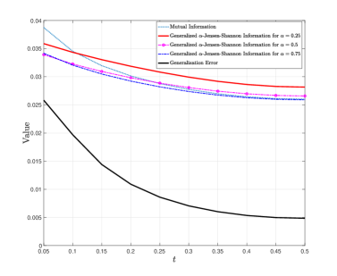
Figure 1: True generalization error, Generalized $\alpha$-Jensen-Shannon based bound for $\alpha=0.25,0.5,0.75$, and Mutual Information based bound.

Fig.2 also depicts the true generalization error, the mutual information based bound in (56), and the $\alpha$-Rényi information based bound for $\alpha=0.25,0.5,0.75$ in (58). It can be seen that the $\alpha$-Rényi based bound is looser than mutual information based bound. If the learning algorithm is a function of some samples, the mutual information based bound is infinite and the $\alpha$-Rényi information based bound is bounded.

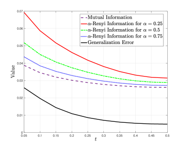
Figure 2: True generalization error, $\alpha$-Rényi based bound for $\alpha=0.25,0.5,0.75$, and Mutual Information based bound.

VI Conclusion and Future Works

We have introduced a new approach to obtain information-theoretic upper bounds on the generalization error associated with supervised learning problems. Our approach can be used to recover the existing bounds and derive new ones based on generalized $\alpha$-Jensen-Shannon, $\alpha$-Rényi information measures. Our upper bounds based on generalized $\alpha$-Jensen-Shannon information measure are bounded by a finite value. Unlike mutual information-based bounds, our upper bound based on $\alpha$-Rényi information for $\alpha\in(0,1)$ under a deterministic learning process is finite-value. Notably, it is shown that the new generalized $\alpha$-Jensen-Shannon information can be tighter in some regimes in comparison to existing bounds.

For future works, we propose the PAC-Bayesian extension of our bounds based on Generalized $\alpha$-Jensen-Shannon and $\alpha$-Rényi divergence for $0<\alpha<1$. The conditional technique based on individual sample measures [18] could also be applied to our upper bounds.

Appendix A Sub-Exponential and Sub-Gamma

We introduce the tail behaviour of two random variables, including sub-Exponential and sub-Gamma.

• Sub-Exponential: A random variable $X$ is $(\sigma_{e}^{2},b)$-sub-Exponential, if $\psi(\lambda)=\frac{\sigma_{e}^{2}\lambda^{2}}{2}$ is an upper bound on $\Lambda_{X}(\lambda)$, for $0\leq|\lambda|\leq\frac{1}{b}$ and $b>0$. Using Lemma 1, we have

  $$\psi^{\star-1}(y)=\begin{cases}&\sqrt{2\sigma_{e}^{2}y},\quad\textit{if }y\leq\frac{\sigma_{e}^{2}}{2b};\\ &by+\frac{\sigma_{e}^{2}}{2b},\quad\textit{otherwise.}\end{cases}$$ (60)

• Sub-Gamma: A random variable $X$ is $\Gamma(\sigma_{s}^{2},c_{s})$-sub-Gamma [50], if $\psi(\lambda)=\frac{\lambda^{2}\sigma_{s}^{2}}{2(1-c_{s}|\lambda|)}$ is an upper bound on $\Lambda_{X}(\lambda)$, for $0<|\lambda|<\frac{1}{c_{s}}$ and $c_{s}>0$. Using Lemma 1, we have

  $$\psi^{\star-1}(y)=\sqrt{2\sigma_{s}^{2}y}+c_{s}y.$$ (61)

Appendix B Proof of Section III-A

B-A Proof of Theorem 3

The proofs of the bounds to $\overline{\operatorname*{gen}}(P_{W|S},\mu)$ and $-\overline{\operatorname*{gen}}(P_{W|S},\mu)$ are similar. We therefore focus on the later.

Let us consider the Donsker–Varadhan variational representation of KL divergence between two probability distributions $\alpha$ and $\beta$ on a common space $\Psi$ given by [51]:

$$D_{\text{KL}}(\alpha\|\beta)=\sup_{f}\int_{\Psi}fd\alpha-\log\int_{\Psi}e^{f}d\beta,$$ (62)

where $f\in\mathcal{F}=\{f:\Psi\rightarrow\mathbb{R}\text{ s.t. }\mathbb{E}_{\beta}[e^{f}]<\infty\}$.

We can now use the Donsker-Varadhan representation to bound $D_{\text{KL}}(P_{W,Z_{i}}\|\widehat{P}_{W,Z_{i}})$ for $\lambda\in(b_{-},0]$ as follows:

$$D_{\text{KL}}(P_{W,Z_{i}}\|\widehat{P}_{W,Z_{i}})\geq$$ (63)

$$\mathbb{E}_{P_{W,Z_{i}}}[\lambda\ell(W,Z_{i})]-\log\mathbb{E}_{\widehat{P}_{W,Z_{i}}}[e^{\lambda\ell(W,{Z}_{i})}]\geq$$

$$\lambda(\mathbb{E}_{P_{W,Z_{i}}}[\ell(W,Z_{i})]-\mathbb{E}_{\widehat{P}_{W,Z_{i}}}[\ell(W,{Z}_{i})])-\psi_{-}(-\lambda),$$ (64)

where the last inequality is due to:

$$\Lambda_{\ell({W},{Z}_{i})}(\lambda)=$$ (65)

$$\log\left(\mathbb{E}_{\widehat{P}_{W,Z_{i}}}[e^{\lambda(\ell(W,{Z}_{i})-\mathbb{E}_{\widehat{P}_{W,Z_{i}}}[\ell(W,{Z}_{i})])}]\right)\leq\psi_{-}(-\lambda).$$

It can then be shown from (64) that the following holds for $\lambda\in(b_{-},0]$:

$$\mathbb{E}_{\widehat{P}_{W,Z_{i}}}[\ell(W,{Z}_{i})]-\mathbb{E}_{{P}_{W,Z_{i}}}[\ell(W,Z_{i})]\leq$$ (66)

$$\inf_{\lambda\in[0,-b_{-})}\frac{D_{\text{KL}}(P_{W,Z_{i}}\|\widehat{P}_{W,Z_{i}})+\psi_{-}(\lambda)}{\lambda}=$$

$$\psi_{-}^{\star-1}(D_{\text{KL}}(P_{W,Z_{i}}\|\widehat{P}_{W,Z_{i}})).$$ (67)

It can likewise also be shown by adopting similar steps that the following holds for $\lambda\in[0,b_{+})$:

$$\mathbb{E}_{P_{W,Z_{i}}}[\ell(W,Z_{i})]-\mathbb{E}_{\widehat{P}_{W,Z_{i}}}[\ell(W,Z_{i})]\leq$$ (68)

$$\inf_{\lambda\in[0,b_{+})}\frac{D_{\text{KL}}(P_{W,Z_{i}}\|\widehat{P}_{W,Z_{i}})+\psi(\lambda)}{\lambda}=$$

$$\psi_{+}^{\star-1}(D_{\text{KL}}(P_{W,Z_{i}}\|\widehat{P}_{W,Z_{i}})).$$ (69)

We can similarly show using an identical procedure that:

$$\mathbb{E}_{P_{W}\otimes\mu}[\ell({W},{Z}_{i})]-\mathbb{E}_{\widehat{P}_{W,Z_{i}}}[\ell(W,\widehat{Z}_{i})]$$

$$\leq\psi_{+}^{\star-1}(D_{\text{KL}}(P_{W}\otimes\mu\|\widehat{P}_{W,Z_{i}}))$$ (70)

$$\mathbb{E}_{\widehat{P}_{W,Z_{i}}}[\ell(W,\widehat{Z}_{i})]-\mathbb{E}_{P_{W}\otimes\mu}[\ell({W},{Z}_{i})]$$

$$\leq\psi_{-}^{\star-1}(D_{\text{KL}}(P_{W}\otimes\mu\|\widehat{P}_{W,Z_{i}})).$$ (71)

Finally, we can immediately bound the generalization error by leveraging (B-A) and (66) as follows:

$$\overline{\operatorname*{gen}}(P_{W|S},\mu)=\frac{1}{n}\sum_{i=1}^{n}\mathbb{E}_{P_{W}\otimes\mu}[\ell({W},{Z}_{i})]-\mathbb{E}_{{P}_{W,Z_{i}}}[\ell(W,Z_{i})]$$

$$=\frac{1}{n}\sum_{i=1}^{n}\mathbb{E}_{P_{W}\otimes\mu}[\ell({W},{Z}_{i})]-\mathbb{E}_{\widehat{P}_{W,Z_{i}}}[\ell({W},{Z}_{i})]+$$

$$~{}\mathbb{E}_{\widehat{P}_{W,Z_{i}}}[\ell({W},{Z}_{i})]-\mathbb{E}_{{P}_{W,Z_{i}}}[\ell(W,Z_{i})]$$

$$\leq\frac{1}{n}\sum_{i=1}^{n}\left(\psi_{+}^{\star-1}(A_{i})+\psi_{-}^{\star-1}(B_{i})\right),$$

where $A_{i}=D_{\text{KL}}(P_{W}\otimes\mu\|\widehat{P}_{W,Z_{i}})$ and $B_{i}=D_{\text{KL}}(P_{W,Z_{i}}\|\widehat{P}_{W,Z_{i}})$.

B-B Proof of Theorem 7

The assumption that the loss function is $\sigma$-sub-Gaussian under the distribution $\widehat{P}_{W,Z_{i}}$ implies that $\psi_{-}^{\star-1}(y)=\psi_{+}^{\star-1}(y)=\sqrt{2\sigma^{2}y}$, [8].

Consider arbitrary auxiliary distributions $\{\widehat{P}_{W,Z_{i}}\}_{i=1}^{n}$ defined on $\mathcal{W}\times\mathcal{Z}$.

$$\overline{\text{\rm{gen}}}(\mu,P_{W|S})=\mathbb{E}_{P_{W}P_{S}}[L_{S}(W)]-\mathbb{E}_{P_{W,S}}[L_{S}(W)]$$

$$=\frac{1}{n}\sum_{i=1}^{n}\mathbb{E}_{P_{W}P_{Z_{i}}}[\ell(W,Z_{i})]-\mathbb{E}_{P_{WZ_{i}}}[\ell(W,Z_{i})]$$ (72)

$$\leq\frac{1}{n}\sum_{i=1}^{n}\left|\mathbb{E}_{P_{W}P_{Z_{i}}}[\ell(W,Z_{i})]-\mathbb{E}_{P_{WZ_{i}}}[\ell(W,Z_{i})]\right|$$ (73)

Using the assumption that the loss function $\ell(w,z_{i})$ is $\sigma_{\alpha}^{2}$-sub-Gaussian under distribution $\widehat{P}_{W,Z_{i}}$ and Donsker-Varadhan representation for $D_{\text{KL}}(P_{WZ_{i}}\|\widehat{P}_{W,Z_{i}})$, we have:

$$\lambda\left(\mathbb{E}_{P_{W,Z_{i}}}[\ell(W,Z_{i})]-\mathbb{E}_{\widehat{P}_{W,Z_{i}}}[\ell(W,Z_{i})]\right)\leq$$ (74)

$$\quad D_{\text{KL}}(P_{WZ_{i}}\|\widehat{P}_{W,Z_{i}})+\frac{\lambda^{2}\sigma_{\alpha}^{2}}{2}.\quad\forall\lambda\in\mathbb{R}$$

Using the assumption loss that the function $\ell(w,z_{i})$ is $\sigma_{\alpha}^{2}$-sub-Gaussian under distribution $\widehat{P}_{W,Z_{i}}$ and Donsker-Varadhan representation for $D_{\text{KL}}(\widehat{P}_{W,Z_{i}}\|P_{W}P_{Z_{i}})$, we have:

$$\lambda^{\prime}\left(\mathbb{E}_{P_{W}P_{Z_{i}}}[\ell(W,Z_{i})]-\mathbb{E}_{\widehat{P}_{W,Z_{i}}}[\ell(W,Z_{i})]\right)\leq$$ (75)

$$\quad D_{\text{KL}}(P_{W}P_{Z_{i}}\|\widehat{P}_{W,Z_{i}})+\frac{{\lambda^{\prime}}^{2}\sigma_{(\alpha)}^{2}}{2}.\quad\forall\lambda^{\prime}\in\mathbb{R}$$

Now if we consider $\lambda<0$, then we can choose $\lambda^{\prime}=\frac{\alpha}{\alpha-1}\lambda$. Hence we have:

$$\mathbb{E}_{\widehat{P}_{W,Z_{i}}}[\ell(W,Z_{i})]-\mathbb{E}_{P_{W,Z_{i}}}[\ell(W,Z_{i})]\leq$$ (76)

$$\quad\frac{D_{\text{KL}}(P_{W,Z_{i}}\|\widehat{P}_{W,Z_{i}})}{|\lambda|}+\frac{|\lambda|\sigma_{\alpha}^{2}}{2}.\quad\forall\lambda\in\mathbb{R^{-}}$$

and,

$$\mathbb{E}_{P_{W}P_{Z_{i}}}[\ell(W,Z_{i})]-\mathbb{E}_{\widehat{P}_{W,Z_{i}}}[\ell(W,Z_{i})]\leq$$ (77)

$$\quad\frac{D_{\text{KL}}(P_{W}P_{Z_{i}}\|\widehat{P}_{W,Z_{i}})}{\lambda^{\prime}}+\frac{\lambda^{\prime}\sigma_{\alpha}^{2}}{2}.\quad\forall\lambda^{\prime}\in\mathbb{R^{+}}$$

Now sum up two Inequalities (76) and (77).

$$\mathbb{E}_{P_{W}P_{Z_{i}}}[\ell(W,Z_{i})]-\mathbb{E}_{P_{WZ_{i}}}[\ell(W,Z_{i})]\leq$$ (78)

$$\frac{\alpha D_{\text{KL}}(P_{W,Z_{i}}\|\widehat{P}_{W,Z_{i}})+(1-\alpha)D_{\text{KL}}(P_{W}P_{Z_{i}}\|\widehat{P}_{W,Z_{i}})}{\alpha|\lambda|}+$$

$$\quad\frac{|\lambda|\sigma_{\alpha}^{2}}{2}+\frac{|\lambda|\frac{\alpha}{1-\alpha}\sigma_{\alpha}^{2}}{2},\quad\forall\lambda\in\mathbb{R^{-}}.$$

Similarly, using an identical approach, we also obtain:

$$-\left(\mathbb{E}_{P_{W}P_{Z_{i}}}[\ell(W,Z_{i})]-\mathbb{E}_{P_{WZ_{i}}}[\ell(W,Z_{i})]\right)\leq$$ (79)

$$\frac{\alpha D_{\text{KL}}(P_{W,Z_{i}}\|\widehat{P}_{W,Z_{i}})+(1-\alpha)D_{\text{KL}}(P_{W}P_{Z_{i}}\|\widehat{P}_{W,Z_{i}})}{\alpha\lambda}+$$

$$\quad\frac{\lambda\sigma_{\alpha}^{2}}{2}+\frac{\lambda\frac{\alpha}{1-\alpha}\sigma_{\alpha}^{2}}{2},\quad\forall\lambda\in\mathbb{R^{+}}.$$

Considering (78) and (79), we have a nonnegative parabola in $\lambda$, whose discriminant must be nonpositive, and we have $\forall\alpha\in(0,1)$:

$$\left|\mathbb{E}_{P_{W}P_{Z_{i}}}[\ell(W,Z_{i})]-\mathbb{E}_{P_{WZ_{i}}}[\ell(W,Z_{i})]\right|^{2}\leq$$ (80)

$$2\sigma_{(\alpha)}^{2}\frac{\left(\alpha D_{\text{KL}}(P_{W,Z_{i}}\|\widehat{P}_{W,Z_{i}})+(1-\alpha)D_{\text{KL}}(P_{W}P_{Z_{i}}\|\widehat{P}_{W,Z_{i}})\right)}{\alpha(1-\alpha)}.$$

Now using (B-B), we prove the claim.

B-C Proof of Lemma 2

$$\alpha D_{\text{KL}}(P_{W}\otimes P_{Z_{i}}\|\widehat{P}_{W,Z_{i}})+(1-\alpha)D_{\text{KL}}(P_{W,Z_{i}}\|\widehat{P}_{W,Z_{i}})$$ (81)

$$=\int_{\mathcal{W}\times\mathcal{Z}}\alpha(dP_{W}\otimes dP_{Z_{i}})\log(dP_{W}\otimes dP_{Z_{i}})$$ (82)

$$\quad+\int_{\mathcal{W}\times\mathcal{Z}}(1-\alpha)dP_{W,Z_{i}}\log(dP_{W,Z_{i}})$$

$$\quad-\int_{\mathcal{W}\times\mathcal{Z}}((\alpha(dP_{W}\otimes dP_{Z_{i}})+(1-\alpha)dP_{W,Z_{i}})\log(d\widehat{P}_{W,Z_{i}}))$$

$$=\int_{\mathcal{W}\times\mathcal{Z}}\alpha(dP_{W}\otimes dP_{Z_{i}})\log(dP_{W}\otimes dP_{Z_{i}})$$ (83)

$$\quad+\int_{\mathcal{W}\times\mathcal{Z}}(1-\alpha)dP_{W,Z_{i}}\log(dP_{W,Z_{i}})-dP_{W,Z_{i}}^{(\alpha)}\log(d\widehat{P}_{W,Z_{i}})$$

$$\quad+\int_{\mathcal{W}\times\mathcal{Z}}dP_{W,Z_{i}}^{(\alpha)}\log(dP_{W,Z_{i}}^{(\alpha)})-dP_{W,Z_{i}}^{(\alpha)}\log(dP_{W,Z_{i}}^{(\alpha)})$$

$$=I_{\textit{JS}}^{\alpha}(W;Z_{i})+D_{\text{KL}}(P_{W,Z_{i}}^{(\alpha)}\|\widehat{P}_{W,Z_{i}}).$$ (84)

B-D Proof of Proposition 8

As shown in [52], and by considering the Lemma 2 we have

$$\min_{\widehat{P}_{W,Z_{i}}}\alpha D_{\text{KL}}(P_{W}\otimes\mu\|\widehat{P}_{W,Z_{i}})+(1-\alpha)D_{\text{KL}}(P_{W,Z_{i}}\|\widehat{P}_{W,Z_{i}})=$$ (85)

$$\min_{\widehat{P}_{W,Z_{i}}}I_{\textit{JS}}^{\alpha}(W;Z_{i})+D_{\text{KL}}(P_{W,Z_{i}}^{(\alpha)}\|\widehat{P}_{W,Z_{i}}).$$

As we have $0\leq D_{\text{KL}}(P_{W,Z_{i}}^{(\alpha)}\|\widehat{P}_{W,Z_{i}})$, therefore, the minimum of (25) is achieved with $\widehat{P}_{W,Z_{i}}=P_{W,Z_{i}}^{(\alpha)}$. Now, considering $\widehat{P}_{W,Z_{i}}=P_{W,Z_{i}}^{(\alpha)}$ in Theorem 7, completes the proof.

B-E Proof of Proposition 12

Using (28),

$$I_{\textit{JS}}^{\alpha}(W;Z_{i})\leq(1-\alpha)I(W;Z_{i}),$$ (86)

we have:

$$|\overline{\operatorname*{gen}}(P_{W|S},\mu)| \leq\frac{1}{n}\sum_{i=1}^{n}\sqrt{2\sigma_{(\alpha)}^{2}\frac{I_{\textit{JS}}^{\alpha}(W;Z_{i})}{\alpha(1-\alpha)}}$$ (87)

$$\leq\frac{1}{n}\sum_{i=1}^{n}\sqrt{2\sigma_{(\alpha)}^{2}\frac{I(W;Z_{i})}{\alpha}}$$ (88)

$$\leq\sqrt{2\sigma_{(\alpha)}^{2}\frac{\sum_{i=1}^{n}I(W;Z_{i})}{\alpha n}}$$ (89)

$$\leq\sqrt{2\sigma_{(\alpha)}^{2}\frac{I(W;S)}{\alpha n}}$$ (90)

$$\leq\sqrt{2\sigma_{(\alpha)}^{2}\frac{H(W)}{\alpha n}},$$ (91)

where the final result, would follow from the finite hypothesis space.

B-F Proof of Proposition 13

This proposition follows from the fact that $I_{\textit{JS}}^{\alpha}(W,Z_{i})\leq h(\alpha)$ for $i=1,\cdots,n$.

Now, we prove that $I_{\textit{JS}}^{\alpha}(W,Z_{i})\leq h(\alpha)$.

$$I_{\textit{JS}}^{\alpha}(W,Z_{i})=$$ (92)

$$\quad\alpha D_{\text{KL}}(P_{W}\otimes P_{Z_{i}}\|P_{W,Z_{i}}^{(\alpha)})+(1-\alpha)D_{\text{KL}}(P_{W,Z_{i}}\|P_{W,Z_{i}}^{(\alpha)})$$

$$=\alpha\int_{\mathcal{W}\times\mathcal{Z}}dP_{W}\otimes dP_{Z_{i}}\log\left(\frac{dP_{W}\otimes dP_{Z_{i}}}{dP_{W,Z_{i}}^{(\alpha)}}\right)$$ (93)

$$\quad+(1-\alpha)\int_{\mathcal{W}\times\mathcal{Z}}dP_{W,Z_{i}}\log\left(\frac{dP_{W,Z_{i}}}{dP_{W,Z_{i}}^{(\alpha)}}\right)$$

$$\leq\alpha\int_{\mathcal{W}\times\mathcal{Z}}dP_{W}\otimes dP_{Z_{i}}\log\left(\frac{dP_{W}\otimes dP_{Z_{i}}}{\alpha(dP_{W}\otimes dP_{Z_{i}})}\right)$$ (94)

$$\quad+(1-\alpha)\int_{\mathcal{W}\times\mathcal{Z}}dP_{W,Z_{i}}\log\left(\frac{dP_{W,Z_{i}}}{(1-\alpha)dP_{W,Z_{i}}}\right)$$

$$=-\alpha\log(\alpha)-(1-\alpha)\log(1-\alpha)$$ (95)

$$=h(\alpha).$$ (96)

B-G Proof of Corollary 14

We first compute the derivative of $\frac{h(\alpha)}{\alpha(1-\alpha)}$ with respect to $\alpha\in(0,1)$

$$\frac{d\frac{h(\alpha)}{\alpha(1-\alpha)}}{d\alpha}=\frac{\log(1-\alpha)}{\alpha^{2}}-\frac{\log(\alpha)}{(1-\alpha)^{2}}.$$ (97)

Now for $\alpha=\frac{1}{2}$, we have $\frac{d\frac{h(\alpha)}{\alpha(1-\alpha)}}{d\alpha}=0$.

Appendix C Proofs of Section III-B

C-A Proof of Proposition 16

Consider arbitrary auxiliary distributions $\{\widehat{P}_{W,Z_{i}}\}_{i=1}^{n}$ defined on $\mathcal{W}\times\mathcal{Z}$. Then,

$$\overline{\operatorname*{gen}}(P_{W|S},\mu)=\mathbb{E}_{P_{W}P_{S}}[L_{S}(W)]-\mathbb{E}_{P_{W,S}}[L_{S}(W)]$$

$$=\frac{1}{n}\sum_{i=1}^{n}\mathbb{E}_{P_{W}P_{Z_{i}}}[\ell(W,Z_{i})]-\mathbb{E}_{P_{WZ_{i}}}[\ell(W,Z_{i})]$$ (98)

$$\leq\frac{1}{n}\sum_{i=1}^{n}\left|\mathbb{E}_{P_{W}P_{Z_{i}}}[\ell(W,Z_{i})]-\mathbb{E}_{P_{WZ_{i}}}[\ell(W,Z_{i})]\right|$$ (99)

$$\leq\frac{1}{n}\sum_{i=1}^{n}\bigl{|}\mathbb{E}_{\widehat{P}_{W,Z_{i}}}[\ell(W,Z_{i})]-\mathbb{E}_{P_{WZ_{i}}}[\ell(W,Z_{i})]\bigr{|}$$ (100)

$$\quad\quad+\bigl{|}\mathbb{E}_{\widehat{P}_{W,Z_{i}}}[\ell(W,Z_{i})]-\mathbb{E}_{P_{W}P_{Z_{i}}}[\ell(W,Z_{i})]\bigr{|}.$$

Using the assumption that loss function $\ell(w,z_{i})$ is $\gamma^{2}$-sub-Gaussian under distribution $P_{W,Z_{i}}$ and Donsker-Varadhan representation we have:

$$\lambda\left(\mathbb{E}_{\widehat{P}_{W,Z_{i}}}[\ell(W,Z_{i})]-\mathbb{E}_{P_{WZ_{i}}}[\ell(W,Z_{i})]\right)\leq$$ (101)

$$\quad D_{\text{KL}}(\widehat{P}_{W,Z_{i}}\|P_{WZ_{i}})+\frac{\lambda^{2}\gamma^{2}}{2},\quad\forall\lambda\in\mathbb{R}.$$

Using the assumption that $\ell(w,Z)$ is $\sigma^{2}$-sub-Gaussian under $P_{W}\otimes P_{Z_{i}}$, and again Donsker-Varadhan representation we have:

$$\lambda^{\prime}\left(\mathbb{E}_{\widehat{P}_{W,Z_{i}}}[\ell(W,Z_{i})]-\mathbb{E}_{P_{W}P_{Z_{i}}}[\ell(W,Z_{i})]\right)\leq$$ (102)

$$\quad D_{\text{KL}}(\widehat{P}_{W,Z_{i}}\|P_{W}P_{Z_{i}})+\frac{{\lambda^{\prime}}^{2}\sigma^{2}}{2}.\quad\forall\lambda^{\prime}\in\mathbb{R}$$

Note that $\mathbb{E}_{P_{W}P_{Z_{i}}}[\ell(W,Z_{i})-\mathbb{E}_{P_{Z_{i}}}[\ell(W,Z_{i})]]=0$.

Now if we consider $\lambda>0$, then we choose $\lambda^{\prime}=\frac{\alpha}{\alpha-1}\lambda$. Hence we have

$$\mathbb{E}_{\widehat{P}_{W,Z_{i}}}[\ell(W,Z_{i})-\mathbb{E}_{P_{W,Z_{i}}}[\ell(W,Z_{i})]]\leq$$ (103)

$$\quad\frac{D_{\text{KL}}(\widehat{P}_{W,Z_{i}}\|P_{WZ_{i}})}{\lambda}+\frac{\lambda\gamma^{2}}{2},\quad\forall\lambda\in\mathbb{R^{+}}.$$

Using the assumption that $\ell(w,Z)$ is $\sigma^{2}$-sub-Gaussian and again Donsker-Varadhan representation,

$$-\mathbb{E}_{\widehat{P}_{W,Z_{i}}}[\ell(W,Z_{i})-\mathbb{E}_{P_{W}P_{Z_{i}}}[\ell(W,Z_{i})]]\leq$$ (104)

$$\quad\frac{D_{\text{KL}}(\widehat{P}_{W,Z_{i}}\|P_{W}P_{Z_{i}})}{|\lambda^{\prime}|}+\frac{|\lambda^{\prime}|\sigma^{2}}{2},\quad\forall\lambda^{\prime}\in\mathbb{R^{-}}.$$

Now sum up two Inequalities (103) and (104), to obtain

$$\mathbb{E}_{P_{W}P_{Z_{i}}}[\ell(W,Z_{i})]-\mathbb{E}_{P_{WZ_{i}}}[\ell(W,Z_{i})]\leq$$ (105)

$$\frac{\alpha D_{\text{KL}}(\widehat{P}_{W,Z_{i}}\|P_{W,Z_{i}})+(1-\alpha)D_{\text{KL}}(\widehat{P}_{W,Z_{i}}\|Q_{W}P_{Z_{i}})}{\alpha\lambda}+$$

$$\quad\frac{\lambda\gamma^{2}}{2}+\frac{\lambda\frac{\alpha}{1-\alpha}\sigma^{2}}{2},\quad\forall\lambda\in\mathbb{R^{+}}.$$

Considering (105), we have a nonnegative parabola in $\lambda$, whose discriminant must be nonpositive, and we have:

$$\left|\mathbb{E}_{P_{W}P_{Z_{i}}}[\ell(W,Z_{i})]-\mathbb{E}_{P_{WZ_{i}}}[\ell(W,Z_{i})]\right|\leq$$ (106)

$$\quad\sqrt{2(\alpha\sigma^{2}+(1-\alpha)\gamma^{2})\frac{\left(\alpha C_{i}+(1-\alpha)D_{i}\right)}{\alpha(1-\alpha)}},$$

where $C_{i}=D_{\text{KL}}(\widehat{P}_{W,Z_{i}}\|P_{W}\otimes\mu)$ and $D_{i}=D_{\text{KL}}(\widehat{P}_{W,Z_{i}}\|P_{W,Z_{i}})$ . Now using (C-A), we prove the claim.

C-B Proof of Proposition 17

Using Lemma 3, we have:

$$\min_{\widehat{P}_{W,Z_{i}}}\alpha D_{\text{KL}}(\widehat{P}_{W,Z_{i}}\|P_{W}\otimes\mu)+(1-\alpha)D_{\text{KL}}(\widehat{P}_{W,Z_{i}}\|P_{W,Z_{i}})=$$ (107)

$$(1-\alpha)I_{R}^{\alpha}(W;Z_{i})$$

$$\quad+\min_{\widehat{P}_{W,Z_{i}}}D_{\text{KL}}\left(\widehat{P}_{W,Z_{i}}\|\frac{(P_{Z_{i}}\otimes P_{W})^{\alpha}(P_{W,Z_{i}})^{(1-\alpha)}}{\int_{\mathcal{W}\times\mathcal{Z}}(dP_{Z_{i}}\otimes dP_{W})^{\alpha}(dP_{W,Z_{i}})^{(1-\alpha)}}\right).$$

Now by considering the $d\widehat{P}_{W,Z_{i}}=\frac{(dP_{Z_{i}}\otimes dP_{W})^{\alpha}(dP_{W,Z_{i}})^{(1-\alpha)}}{\int_{\mathcal{W}\times\mathcal{Z}}(dP_{Z_{i}}\otimes dP_{W})^{\alpha}(dP_{W,Z_{i}})^{(1-\alpha)}}$, the KL term would be equal to zero. Now, using Proposition 16, we prove the final result.

C-C Proof of Lemma 3

Our proof is based on [40, Theorem 30]. For $0\leq\alpha\leq 1$, we have:

$$\alpha D_{\text{KL}}(\widehat{P}_{W,Z_{i}}\|P_{W}\otimes\mu)+(1-\alpha)D_{\text{KL}}(\widehat{P}_{W,Z_{i}}\|P_{W,Z_{i}})$$ (108)

$$=\int_{\mathcal{W}\times\mathcal{Z}}d\widehat{P}_{W,Z_{i}}\log(d\widehat{P}_{W,Z_{i}})$$ (109)

$$\quad-\int_{\mathcal{W}\times\mathcal{Z}}\widehat{P}_{W,Z_{i}}\log((dP_{W}\otimes dP_{Z_{i}})^{\alpha}(dP_{W,Z_{i}})^{(1-\alpha)})$$

$$=\int_{\mathcal{W}\times\mathcal{Z}}d\widehat{P}_{W,Z_{i}}\log(d\widehat{P}_{W,Z_{i}})$$ (110)

$$\quad-\int_{\mathcal{W}\times\mathcal{Z}}d\widehat{P}_{W,Z_{i}}\log\left((dP_{W}\otimes dP_{Z_{i}})^{\alpha}(dP_{W,Z_{i}})^{(1-\alpha)}\right)$$

$$\quad+\log\left(\int_{\mathcal{W}\times\mathcal{Z}}(dP_{W}\otimes dP_{Z_{i}})^{\alpha}(dP_{W,Z_{i}})^{(1-\alpha)}\right)$$

$$\quad-\log\left(\int_{\mathcal{W}\times\mathcal{Z}}(dP_{W}\otimes dP_{Z_{i}})^{\alpha}(dP_{W,Z_{i}})^{(1-\alpha)}\right)$$

$$=-\log\left(\int_{\mathcal{W}\times\mathcal{Z}}(P_{W}\otimes dP_{Z_{i}})^{\alpha}(dP_{W,Z_{i}})^{(1-\alpha)}\right)$$ (111)

$$\quad+\int_{\mathcal{W}\times\mathcal{Z}}d\widehat{P}_{W,Z_{i}}\log(d\widehat{P}_{W,Z_{i}})$$

$$\quad-\int_{\mathcal{W}\times\mathcal{Z}}d\widehat{P}_{W,Z_{i}}\log\left(\frac{(dP_{W}\otimes dP_{Z_{i}})^{\alpha}(dP_{W,Z_{i}})^{(1-\alpha)}}{\int_{\mathcal{W}\times\mathcal{Z}}(dP_{W}\otimes dP_{Z_{i}})^{\alpha}(dP_{W,Z_{i}})^{(1-\alpha)}}\right)$$

$$=(1-\alpha)I_{R}^{\alpha}(W;Z_{i})$$ (112)

$$\quad+D_{\text{KL}}\left(\widehat{P}_{W,Z_{i}}\|\frac{(P_{Z_{i}}\otimes P_{W})^{\alpha}(P_{W,Z_{i}})^{(1-\alpha)}}{\int_{\mathcal{W}\times\mathcal{Z}}(dP_{Z_{i}}\otimes dP_{W})^{\alpha}(dP_{W,Z_{i}})^{(1-\alpha)}}\right).$$

C-D Proof of Proposition 22

Using (39),

$$I_{R}^{\alpha}(W;Z_{i})\leq\frac{\alpha}{1-\alpha}I(W;Z_{i}),$$ (113)

and considering the hypothesis space is countable and the upper bound in Proposition 17 we have:

$$|\overline{\operatorname*{gen}}(P_{W|S},\mu)|\leq\frac{1}{n}\sum_{i=1}^{n}\sqrt{2(\alpha\sigma^{2}+(1-\alpha)\gamma^{2})\frac{I_{R}^{\alpha}(W;Z_{i})}{\alpha}}$$ (114)

$$\leq\frac{1}{n}\sum_{i=1}^{n}\sqrt{2(\alpha\sigma^{2}+(1-\alpha)\gamma^{2})\min\left\{\frac{1}{\alpha},\frac{1}{1-\alpha}\right\}I(W;Z_{i})}$$ (115)

$$\leq\sqrt{2(\alpha\sigma^{2}+(1-\alpha)\gamma^{2})\min\left\{\frac{1}{\alpha},\frac{1}{1-\alpha}\right\}\frac{\sum_{i=1}^{n}I(W;Z_{i})}{n}}$$ (116)

$$\leq\sqrt{2(\alpha\sigma^{2}+(1-\alpha)\gamma^{2})\min\left\{\frac{1}{\alpha},\frac{1}{1-\alpha}\right\}\frac{I(W;S)}{n}}$$ (117)

$$\leq\sqrt{2(\alpha\sigma^{2}+(1-\alpha)\gamma^{2})\min\left\{\frac{1}{\alpha},\frac{1}{1-\alpha}\right\}\frac{H(W)}{n}}$$ (118)

$$\quad\leq\sqrt{2(\alpha\sigma^{2}+(1-\alpha)\gamma^{2})\min\left\{\frac{1}{\alpha},\frac{1}{1-\alpha}\right\}\frac{\log(k)}{n}},$$

where (116) follows from Jensen inequality and (117) follows from i.i.d assumption for $Z_{i}$’s.

C-E Proof of Theorem 23

Consider arbitrary auxiliary distributions $\{\tilde{P}_{WZ_{i}}\}_{i=1}^{n}$ defined on $\mathcal{W}\times\mathcal{Z}$.

$$\overline{\operatorname*{gen}}(P_{W|S},\mu)=\mathbb{E}_{P_{W}P_{S}}[L_{S}(W)]-\mathbb{E}_{P_{W,S}}[L_{S}(W)]$$

$$=\frac{1}{n}\sum_{i=1}^{n}\mathbb{E}_{P_{W}P_{Z_{i}}}[\ell(W,Z_{i})]-\mathbb{E}_{P_{WZ_{i}}}[\ell(W,Z_{i})]$$ (119)

$$\leq\frac{1}{n}\sum_{i=1}^{n}\left|\mathbb{E}_{P_{W}P_{Z_{i}}}[\ell(W,Z_{i})]-\mathbb{E}_{P_{WZ_{i}}}[\ell(W,Z_{i})]\right|.$$ (120)

Using the assumption centered loss function $\ell(w,z_{i})-\mathbb{E}_{P_{Z_{i}}}[\ell(w,Z_{i})]$ is $\gamma^{2}$-sub-Gaussian under distribution $P_{WZ_{i}}$ and Donsker-Varadhan representation by considering function $\ell(w,z_{i})-\mathbb{E}_{P_{Z_{i}}}[\ell(w,Z_{i})]$ we have:

$$\lambda\bigg{(}\mathbb{E}_{\tilde{P}_{WZ_{i}}}[\ell(W,Z_{i})-\mathbb{E}_{P_{Z_{i}}}[\ell(W,Z_{i})]]$$ (121)

$$\quad-\mathbb{E}_{P_{WZ_{i}}}[\ell(W,Z_{i})-\mathbb{E}_{P_{Z_{i}}}[\ell(W,Z_{i})]]\bigg{)}$$

$$\leq D_{\text{KL}}(\tilde{P}_{WZ_{i}}\|P_{WZ_{i}})+\frac{\lambda^{2}\gamma^{2}}{2}.\quad\forall\lambda\in\mathbb{R}$$

Note that $\mathbb{E}_{P_{WZ_{i}}}[\ell(W,Z_{i})-\mathbb{E}_{P_{Z_{i}}}[\ell(W,Z_{i})]]=\mathbb{E}_{P_{WZ_{i}}}[\ell(W,Z_{i})]-\mathbb{E}_{P_{W}P_{Z_{i}}}[\ell(W,Z_{i})]$.

Using the assumption that $\ell(w,Z)$ is $\sigma^{2}$-sub-Gaussian under $P_{Z_{i}}$ for all $w\in\mathcal{W}$, and again Donsker-Varadhan representation by considering function $\ell(w,z_{i})-\mathbb{E}_{P_{Z_{i}}}[\ell(w,Z_{i})]$ we have:

$$\lambda^{\prime}\bigg{(}\mathbb{E}_{\tilde{P}_{WZ_{i}}}[\ell(W,Z_{i})-\mathbb{E}_{P_{Z_{i}}}[\ell(W,Z_{i})]]$$ (122)

$$\quad-\mathbb{E}_{Q_{W}P_{Z_{i}}}[\ell(W,Z_{i})-\mathbb{E}_{P_{Z_{i}}}[\ell(W,Z_{i})]]\bigg{)}$$

$$\quad\leq D_{\text{KL}}(\tilde{P}_{WZ_{i}}\|Q_{W}P_{Z_{i}})+\frac{{\lambda^{\prime}}^{2}\sigma^{2}}{2}.\quad\forall\lambda^{\prime}\in\mathbb{R}$$

Note that $\mathbb{E}_{Q_{W}P_{Z_{i}}}[\ell(W,Z_{i})-\mathbb{E}_{P_{Z_{i}}}[\ell(W,Z_{i})]]=0$.

Now if we consider $\lambda>0$, then we choose $\lambda^{\prime}=\frac{\alpha}{\alpha-1}\lambda$. Hence we have

$$\mathbb{E}_{\tilde{P}_{WZ_{i}}}[\ell(W,Z_{i})-\mathbb{E}_{P_{Z_{i}}}[\ell(W,Z_{i})]]$$ (123)

$$\quad-\mathbb{E}_{P_{WZ_{i}}}[\ell(W,Z_{i})-\mathbb{E}_{P_{Z_{i}}}[\ell(W,Z_{i})]]$$

$$\quad\leq\frac{D_{\text{KL}}(\tilde{P}_{WZ_{i}}\|P_{WZ_{i}})}{\lambda}+\frac{\lambda\gamma^{2}}{2},\quad\forall\lambda\in\mathbb{R^{+}}.$$

Using the assumption $\ell(w,Z)$ is $\sigma^{2}$-sub-Gaussian and again Donsker-Varadhan representation,

$$-\mathbb{E}_{\tilde{P}_{WZ_{i}}}[\ell(W,Z_{i})-\mathbb{E}_{P_{Z_{i}}}[\ell(W,Z_{i})]]\leq$$ (124)

$$\quad\frac{D_{\text{KL}}(\tilde{P}_{WZ_{i}}\|Q_{W}P_{Z_{i}})}{|\lambda^{\prime}|}+\frac{|\lambda^{\prime}|\sigma^{2}}{2},\quad\forall\lambda^{\prime}\in\mathbb{R^{-}}.$$

Now sum up the two Inequalities (123) and (124) to obtain,

$$\mathbb{E}_{P_{W}P_{Z_{i}}}[\ell(W,Z_{i})]-\mathbb{E}_{P_{WZ_{i}}}[\ell(W,Z_{i})]\leq$$ (125)

$$\frac{\alpha D_{\text{KL}}(\tilde{P}_{WZ_{i}}\|P_{WZ_{i}})+(1-\alpha)D_{\text{KL}}(\tilde{P}_{WZ_{i}}\|Q_{W}P_{Z_{i}})}{\alpha\lambda}+$$

$$\quad\frac{\lambda\gamma^{2}}{2}+\frac{\lambda\frac{\alpha}{1-\alpha}\sigma^{2}}{2},\quad\forall\lambda\in\mathbb{R^{+}}.$$

Taking infimum on $\tilde{P}_{WZ_{i}}$ and using [40, Theorem 30] that states

$$(1-\alpha)D_{\alpha}(P_{1}\|P_{2})=\inf_{R}\{\alpha D_{\text{KL}}(R\|P_{1})+(1-\alpha)D_{\text{KL}}(R\|P_{2})\}$$

Now, we have:

$$(1-\alpha)D_{\alpha}(P_{WZ_{i}}\|Q_{W}P_{Z_{i}})=$$ (126)

$${\inf_{\tilde{P}_{WZ_{i}}}\{\alpha D_{\text{KL}}(\tilde{P}_{WZ_{i}}\|P_{WZ_{i}})+(1-\alpha)D_{\text{KL}}(\tilde{P}_{WZ_{i}}\|Q_{W}P_{Z_{i}})\}}$$

and taking infimum on $Q_{W}$, we have:

$$\inf_{Q_{W}}D_{\alpha}(P_{WZ_{i}}\|Q_{W}P_{Z_{i}})=I_{S}^{\alpha}(Z_{i};W).$$ (127)

Using (127) in (125), we get:

$$\mathbb{E}_{P_{W}P_{Z_{i}}}[\ell(W,Z_{i})]-\mathbb{E}_{P_{WZ_{i}}}[\ell(W,Z_{i})]\leq$$ (128)

$$\quad\frac{(1-\alpha)I^{s}_{\alpha}(Z_{i};W)}{\lambda\alpha}+\frac{\lambda\gamma^{2}}{2}+\frac{\lambda\frac{\alpha}{1-\alpha}\sigma^{2}}{2}\quad\forall\lambda\in\mathbb{R^{+}}.$$

Using the same approach for $\lambda\in R^{-}$, we have:

$$\mathbb{E}_{P_{WZ_{i}}}[\ell(W,Z_{i})]-\mathbb{E}_{P_{W}P_{Z_{i}}}[\ell(W,Z_{i})]\leq$$ (129)

$$\quad\frac{(1-\alpha)I^{s}_{\alpha}(Z_{i};W)}{|\lambda|\alpha}+\frac{|\lambda|\gamma^{2}}{2}+\frac{|\lambda|\frac{\alpha}{1-\alpha}\sigma^{2}}{2},\quad\forall\lambda\in\mathbb{R^{-}}.$$

Considering (128) and (129), we have a nonnegative parabola in $\lambda$, whose discriminant must be nonpositive, and we have:

$$\left|\mathbb{E}_{P_{W}P_{Z_{i}}}[\ell(W,Z_{i})]-\mathbb{E}_{P_{WZ_{i}}}[\ell(W,Z_{i})]\right|\leq$$ (130)

$$\quad\sqrt{2(\alpha\sigma^{2}+(1-\alpha)\gamma^{2})\frac{I_{S}^{\alpha}(Z_{i};W)}{\alpha}}.$$

Now using (C-A), we prove the claim.

C-F Proof of Proposition 24

There is a generalization of Pinsker’s inequality in [40] as follows:

Theorem 32 (generalization of Pinsker’s inequality)

$$\|P-Q\|^{2}_{TV}\leq\frac{2}{\alpha}D_{\alpha}(P\|Q),\quad\alpha\in(0,1]$$ (131)

Denote $f:\mathcal{X}\to\mathbb{R}$ a bounded function $|f|\leq L$, then

$$\mathbb{E}_{P}[f(X)]-\mathbb{E}_{Q}[f(X)]=$$ (132)

$$\quad\int f(x)(P(dx)-Q(dx))\leq$$

$$\quad\sup_{x}f(x)\cdot\int|P(dx)-Q(dx)|\leq L\sqrt{\frac{2}{\alpha}D_{\alpha}(P\|Q)}.$$

Let $P=P_{W,S}$, $Q=P_{W}P_{S}$ and $f(w,s)=L_{\mu}(w)-L_{s}(w)$. Then, we have the final result,

$$\overline{\operatorname*{gen}}(P_{W|S},\mu)=\mathbb{E}[L_{\mu}(W)-L_{S}]\leq\sqrt{\frac{2b^{2}}{n\alpha}D_{\alpha}(P_{W,S}\|P_{W}P_{S})}$$ (133)

C-G Proof of Proposition 26

It can be shown that the symmetrized KL information can be written as

$$I_{\mathrm{SKL}}(W;S)=\mathbb{E}_{P_{W,S}}[\log(P_{W|S}^{\alpha})]-\mathbb{E}_{P_{W}\otimes P_{S}}[\log(P_{W|S}^{\alpha})].$$ (134)

Note that $P_{W,S}$ and $P_{W}\otimes P_{S}$ share the same marginal distribution, hence we have $\mathbb{E}_{P_{W,S}}[\log\pi(W)]=\mathbb{E}_{P_{W}}[\log\pi(W)]$, and $\mathbb{E}_{P_{W,S}}[\log V(S,\alpha)]=\mathbb{E}_{P_{S}}[\log V(S,\alpha)]$. Then, combining the following Gibbs algorithm,

$$P^{[\alpha]}_{W|S=s}(dw)=\frac{e^{\frac{-\beta}{\min\{1,\frac{\alpha}{1-\alpha}\}}[L_{s}(w)]}Q_{W}(dw)}{\mathbb{E}_{Q_{W}}\left[e^{\frac{-\beta}{\min\{1,\frac{\alpha}{1-\alpha}\}}[L_{s}(w)]}\right]},$$ (135)

with (134) completes the proof.

Appendix D Proof of Proposition 27

It follows from

$$I_{\textit{JS}}^{\alpha}(W;Z_{i})\leq\frac{h(\alpha^{\prime})}{\alpha^{\prime}(1-\alpha^{\prime})},$$

that if we have $\frac{\alpha h(\alpha^{\prime})}{\alpha^{\prime}(1-\alpha^{\prime})}\leq I_{R}^{\alpha}(W;Z_{i})$ for all $i=1,\cdots,n$, then the results holds for $\sigma=\gamma=\sigma_{JS}$.

Appendix E Proof of Section IV

We first propose the following Lemma to provide an upper bound on the expected generalization error under distribution mismatch.

Lemma 5

The following upper bound holds on expected generalization error under distribution mismatch between the test and training distributions:

$$|\overline{\operatorname*{gen}}(P_{W|S},\mu,\mu^{\prime})|\leq$$ (136)

$$\quad|\overline{\operatorname*{gen}}(P_{W|S},\mu)|+|\mathbb{E}_{P_{W}\otimes\mu^{\prime}}[\ell(W,Z)]-\mathbb{E}_{P_{W}\otimes\mu}[\ell(W,Z)]|.$$

Proof:

We have:

$$|\overline{\operatorname*{gen}}(P_{W|S},\mu,\mu^{\prime})|$$ (137)

$$=|\mathbb{E}_{P_{W,S}}[L_{P}(W,\mu^{\prime})-L_{P}(W,\mu)+L_{P}(W,\mu)-L_{E}(E,S)]|$$

$$\leq|\mathbb{E}_{P_{W,S}}[L_{P}(W,\mu^{\prime})-L_{P}(W,\mu)]|+|\overline{\operatorname*{gen}}(P_{W|S},\mu)|$$

$$=|\mathbb{E}_{P_{W}\otimes\mu^{\prime}}[\ell(W,Z)]-\mathbb{E}_{P_{W}\otimes\mu}[\ell(W,Z)]|+|\overline{\operatorname*{gen}}(P_{W|S},\mu)|$$

∎

E-A Proof of Proposition 30

In Lemma 5, the generalization error under distribution mismatch can be upper bounded by two terms. Considering Proposition 8, we can provide the upper bound based on generalized $\alpha$-Jensen-Shannon information over $|\overline{\operatorname*{gen}}(P_{W|S},\mu)|$. We can also provide an upper bound on the term $|\mathbb{E}_{P_{W}\otimes\mu^{\prime}}[\ell(W,Z)]-\mathbb{E}_{P_{W}\otimes\mu}[\ell(W,Z)]|$ in Lemma 5 by applying ADM using a similar approach as in Proposition 8 and using the generalized $\alpha$-Jensen-Shannon divergence as follows:

$$|\mathbb{E}_{P_{W}\otimes\mu^{\prime}}[\ell(W,Z)]-\mathbb{E}_{P_{W}\otimes\mu}[\ell(W,Z)]|\leq$$ (138)

$$\sqrt{2\sigma_{(\alpha)}^{2}\frac{D_{\text{JS}}^{\alpha}(P_{W}\otimes\mu^{\prime}\|P_{W}\otimes\mu)}{\alpha(1-\alpha)}}=$$ (139)

$$\sqrt{2\sigma_{(\alpha)}^{2}\frac{D_{\text{JS}}^{\alpha}(\mu^{\prime}\|\mu)}{\alpha(1-\alpha)}}.$$ (140)

E-B Proof of Proposition 31

Based on Lemma 5, the generalization error is upper bounded by two terms (See Equation (136)). We can provide the upper bound based on $\alpha$-Rényi information over $|\overline{\operatorname*{gen}}(P_{W|S},\mu)|$ using Proposition 17. We can also provide an upper bound on the term $|\mathbb{E}_{P_{W}\otimes\mu^{\prime}}[\ell(W,Z)]-\mathbb{E}_{P_{W}\otimes\mu}[\ell(W,Z)]|$ by applying ADM using a similar approach as in Proposition 17 and using $\alpha$-Rényi divergence as follows:

$$|\mathbb{E}_{P_{W}\otimes\mu^{\prime}}[\ell(W,Z)]-\mathbb{E}_{P_{W}\otimes\mu}[\ell(W,Z)]|\leq$$ (141)

$$\sqrt{2(\alpha\sigma^{2}+(1-\alpha)\gamma^{2})\frac{D_{\alpha}(P_{W}\otimes\mu^{\prime}\|P_{W}\otimes\mu)}{\alpha}}=$$ (142)

$$\sqrt{2(\alpha\sigma^{2}+(1-\alpha)\gamma^{2})\frac{D_{\alpha}(\mu^{\prime}\|\mu)}{\alpha}}.$$ (143)

Appendix F Generalization Error Upper Bounds Based on $\alpha$-KL-Pythagorean and Triangular Discrimination Measures

In this section, we provide an upper bound based on a new divergence measure, $\alpha$-KL-Pythagorean divergence, which is inspired by the Pythagorean inequality for KL divergence. We also provide an upper bound based on triangular Discrimination by applying auxiliary distribution to Chi-square divergence. The upper bound based on triangular Discrimination is also finite.

The triangular Discrimination measure has been employed in many machine learning problems including PAC-Bayesian learning, [53] and surrogate loss functions [54].

F-A Preliminaries

In our characterization of generalization error upper bounds in this section, we will use the information measures between two distributions $P_{X}$ and $P_{X^{\prime}}$ on a common measurable space $\mathcal{X}$ in Table IV. The new measure $\alpha$-KL-Pythagorean divergence can be characterized by a convex combination of KL-divergences as defined in Definition (149). Chi-square divergence and Triangular Discrimination are other divergences that are related to our discussion on the ADM (See Sections F-C). The information measures based on these divergences are summarized in Table V.

TABLE IV: Divergence Measures Definitions

Divergence Measure	Definition
$\alpha$-KL-Pythagorean divergence (new measure)	$K_{\alpha}(P_{X}\|P_{X^{\prime}})\triangleq\inf_{Q_{X}\in\mathbb{P}(\mathcal{X})}\alpha D_{\text{KL}}(P_{X}\|Q_{X})+(1-\alpha)D_{\text{KL}}(Q_{X}\|P_{X^{\prime}})$
Chi-square divergence [56]	$\chi^{2}(P_{X}\|P_{X^{\prime}})\triangleq\int_{\mathcal{X}}\frac{(P_{X}(x)-P_{X^{\prime}}(x))^{2}}{P_{X^{\prime}}(x)}dx$
Triangular Discrimination [34]	$\Delta(P_{X}\|P_{X^{\prime}})\triangleq\int_{\mathcal{X}}\frac{(P_{X}(x)-P_{X^{\prime}}(x))^{2}}{P_{X}(x)+P_{X^{\prime}}(x)}dx$

TABLE V: Information Measures Definitions

Information Measure	Definition
Triangular Discrimination information	$I_{\Delta}(X;X^{\prime})\triangleq\Delta(P_{X,X^{\prime}}\|P_{X}\otimes P_{X^{\prime}})$
$\alpha$-KL-Pythagorean information	$I_{K_{\alpha}}(X;X^{\prime})\triangleq K_{\alpha}(P_{X,X^{\prime}}\|P_{X}\otimes P_{X^{\prime}})$

F-B $\alpha$-KL-Pythagorean Based Upper bound

We now provide a different generalization bound, relying on KL divergence terms $D_{\text{KL}}(\widehat{P}_{W,Z_{i}}\|P_{W}\otimes\mu)$ and $D_{\text{KL}}(P_{W,Z_{i}}\|\widehat{P}_{W,Z_{i}})$, where $\hat{P}_{W,Z_{i}}$ is an auxiliary distribution, that can be ultimately expressed in terms of a new divergence measure that we will also discuss in the sequel.

Corollary 33

Considering the same assumptions in Theorem 3 and Proposition 15, the following expected generalization error upper bounds hold:

$$\overline{\operatorname*{gen}}(P_{W|S},\mu)\leq\frac{1}{n}\sum_{i=1}^{n}\left(\psi_{+}^{\star-1}(B_{i})+\phi_{+}^{\star-1}(D_{i})\right),$$ (144)

$$-\overline{\operatorname*{gen}}(P_{W|S},\mu)\leq\frac{1}{n}\sum_{i=1}^{n}\left(\psi_{-}^{\star-1}(B_{i})+\phi_{-}^{\star-1}(D_{i})\right),$$ (145)

where $B_{i}=D_{\text{KL}}(P_{W,Z_{i}}\|\widehat{P}_{W,Z_{i}})$, and $D_{i}=D_{\text{KL}}(\widehat{P}_{{W},{Z}_{i}}\|P_{W}\otimes\mu)$.

Proof:

The proof is straightforward and similar to Theorem 3. ∎

In Section III-A, we provided generalized $\alpha$-Jensen-Shannon information based upper bound using the following convex combination of two KL divergences terms,

$$D^{\alpha}_{JS}(P\|Q)=\min_{R}\alpha D_{\text{KL}}(P\|R)+(1-\alpha)D_{\text{KL}}(Q\|R),$$ (146)

In turn, in Section III-B, the $\alpha$-Rényi based upper bound is derived by using the following convex combination of two KL divergences terms,

$$(1-\alpha)D_{\alpha}(P\|Q)=$$ (147)

$$\quad\min_{R}\alpha D_{\text{KL}}(R\|P)+(1-\alpha)D_{\text{KL}}(R\|Q).$$

Now, we define a new divergence measure inspired by the following convex combination of KL divergence terms:

$$\alpha D_{\text{KL}}(P\|R)+(1-\alpha)D_{\text{KL}}(R\|Q).$$ (148)

Definition 34

Assume $P\ll Q$. Then, the $\alpha$-KL-Pythagorean divergence is defined as follows:

$$K_{\alpha}(P\|Q)\triangleq\inf_{R\in\mathbb{P}(\mathcal{X})}\alpha D_{\text{KL}}(P\|R)+(1-\alpha)D_{\text{KL}}(R\|Q).$$ (149)

We will be assuming that $K_{\alpha}(P\|Q)$ is well-defined i.e. there is a unique minimizer $R\in\mathbb{P}(\mathcal{X})$, where $\mathbb{P}(\mathcal{X})$ is the set of all probability distributions over space $\mathcal{X}$.

Note that for many sample spaces $\mathcal{X}$ (E.g. compact metric space), $\mathbb{P}(\mathcal{X})$ is a closed set under some topology. Therefore, the optimization problem in (149)) is convex, exhibiting a unique solution.

We provide the main properties of $\alpha$-KL-Pythagorean divergence in the following Theorem.

Theorem 35

The $\alpha$-KL-Pythagorean divergence has the following properties:

1. Non-negativity: $K_{\alpha}(P\|Q)\geq 0$ and equality holds if and only if $P=Q$.

2. Joint convexity: $K_{\alpha}(P\|Q)$ is a jointly convex function of $(P,Q)$.

3. Monotonicity: $K_{\alpha}(P_{XY}\|Q_{XY})\geq K_{\alpha}(P_{X}\|Q_{X})$.

4. Data processing: Consider a channel that produces $Y$ given $X$ based on the conditional law $P_{Y|X}$. Let $P_{Y}$ (resp. $Q_{Y}$) denote the distribution of $Y$ when $X$ is distributed as $P_{X}$ (resp. $Q_{X}$), then

   $$K_{\alpha}(P_{Y}\|Q_{Y})\leq K_{\alpha}(P_{X}\|Q_{X}).$$

5. Supermodularity: Let $P_{X}\xrightarrow[]{P_{Y|X}}P_{Y}$ and $Q_{XY}=Q_{X}Q_{Y}$. Then

   $$K_{\alpha}(P_{XY}\|Q_{XY})\geq K_{\alpha}(P_{X}\|Q_{X})+K_{\alpha}(P_{Y}\|Q_{Y}).$$

Proof:

Proof of (i): If $\alpha=0\,\,\text{\rm{or}}\,\,1$, the claim is obvious. Otherwise, non-negativity of $K_{\alpha}$ follows from non-negativity of KL-divergence. $K_{\alpha}(P\|Q)=0$ iff there exist distribution $R$ such that $D_{\text{KL}}(P\|R)=0$ and $D_{\text{KL}}(R\|Q)=0$. The only way is $P=Q$.

Proof of (ii): Let define

$$K_{\alpha}(P,Q,R):=\alpha D_{\text{KL}}(P\|R)+(1-\alpha)D_{\text{KL}}(R\|Q).$$

Consider $(P_{1},Q_{1},R_{1})$ and $(P_{2},Q_{2},R_{2})$ are two points in $\mathbb{P}(\mathcal{X})\times\mathbb{P}(\mathcal{X})\times\mathbb{P}(\mathcal{X})$.

$$K_{\alpha}(\alpha P_{1}+(1-\alpha)P_{2},\alpha Q_{1}+(1-\alpha)Q_{2},\alpha R_{1}+(1-\alpha)R_{2})$$

$$=\alpha D_{\text{KL}}(\beta P_{1}+(1-\beta)P_{2}\|\alpha R_{1}+(1-\alpha)R_{2})$$ (150)

$$\quad+(1-\alpha)D_{\text{KL}}(\alpha R_{1}+(1-\alpha)R_{2}\|\beta Q_{1}+(1-\beta)Q_{2})$$

$$\overset{(a)}{\leq}\beta\bigg{[}\alpha D_{\text{KL}}(P_{1}\|R_{1})+(1-\alpha)D_{\text{KL}}(R_{1}\|Q_{1})\bigg{]}$$ (151)

$$\quad+(1-\beta)\left[\alpha D_{\text{KL}}(P_{2}\|R_{2})+(1-\alpha)D_{\text{KL}}(R_{2}\|P_{2})\right]$$

$$=\beta K_{\alpha}(P_{1},Q_{1},R_{1})+(1-\beta)K_{\alpha}(P_{2},Q_{2},R_{2}),$$ (152)

where (a) comes from jointly convexity of KL-divergence. So $K_{\alpha}(P,Q,R)$ is a jointly convex function of $(P,Q,R)$. We know from the elementary convex analysis that $\min_{a\in\mathcal{A}}\phi(a,b)$ is convex when $\phi(a,b)$ is jointly convex function of $(a,b)$ and $\mathcal{A}$ is a convex set. So $K_{\alpha}(P\|Q)=\inf_{R\in\mathbb{P}(\mathcal{X})}K_{\alpha}(P,Q,R)$ is a convex function of $(P,Q)$.

Proof of (iii):

$$K_{\alpha}(P_{XY}\|Q_{XY})=$$ (153)

$$\quad\inf_{R_{XY}\in\mathbb{P}(\mathcal{X}\times\mathcal{Y})}\alpha D_{\text{KL}}(P_{XY}\|R_{XY})+(1-\alpha)D_{\text{KL}}(R_{XY}\|Q_{XY})$$

$$\overset{(a)}{\geq}\inf_{R_{XY}\in\mathbb{P}(\mathcal{X}\times\mathcal{Y})}\alpha D_{\text{KL}}(P_{X}\|R_{X})+(1-\alpha)D_{\text{KL}}(R_{X}\|Q_{X})$$ (154)

$$\quad=K_{\alpha}(P_{X}\|Q_{X}),$$

where (a) comes from monotonicity of KL divergence $D_{\text{KL}}(P_{XY}\|Q_{XY})\geq D_{\text{KL}}(P_{X}\|Q_{X})$.

Proof of (iv):

$$K_{\alpha}(P_{Y}\|Q_{Y})$$ (155)

$$\quad\overset{(a)}{\leq}K_{\alpha}(P_{XY}\|Q_{XY})=K_{\alpha}(P_{X}P_{Y|X}\|Q_{X}P_{Y|X})$$

$$=\inf_{R_{XY}\in\mathbb{P}(\mathcal{X}\times\mathcal{Y})}\alpha D_{\text{KL}}(P_{X}P_{Y|X}\|R_{XY})$$ (156)

$$+(1-\alpha)D_{\text{KL}}(R_{XY}\|Q_{X}P_{Y|X})$$

$$\overset{(b)}{\leq}\inf_{R_{X}\in\mathbb{P}(\mathcal{X})}\alpha D_{\text{KL}}(P_{X}P_{Y|X}\|R_{X}P_{Y|X})$$ (157)

$$+(1-\alpha)D_{\text{KL}}(R_{X}P_{Y|X}\|Q_{X}P_{Y|X})$$

$$=K_{\alpha}(P_{X}\|Q_{X}),$$ (158)

where (a) comes from Part (iii) and (b) is derived by considering a smaller subset of the joint distribution like $R_{XY}=R_{X}P_{Y|X}$ in the general minimization. The last equality is derived from chain rule for KL divergence.

Proof of (v):

$$K_{\alpha}(P_{XY}\|Q_{XY})=$$ (159)

$$\quad\inf_{R_{XY}\in\mathbb{P}(\mathcal{X}\times\mathcal{Y})}\alpha D_{\text{KL}}(P_{XY}\|R_{XY})+(1-\alpha)D_{\text{KL}}(R_{XY}\|Q_{XY})$$

$$\overset{(a)}{\geq}\inf_{R_{XY}\in\mathbb{P}(\mathcal{X}\times\mathcal{Y})}\alpha[D_{\text{KL}}(P_{X}\|R_{X})+D_{\text{KL}}(P_{Y}\|R_{Y})]$$ (160)

$$\quad+(1-\alpha)[D_{\text{KL}}(R_{X}\|Q_{X})+D_{\text{KL}}(R_{Y}\|P_{Y})]$$

$$\overset{(b)}{\geq}\inf_{R_{X}\in\mathbb{P}(\mathcal{X})}\alpha D_{\text{KL}}(P_{X}\|R_{X})+(1-\alpha)D_{\text{KL}}(R_{X}\|Q_{X})$$ (161)

$$\quad+\inf_{R_{Y}\in\mathbb{P}(\mathcal{Y})}\alpha D_{\text{KL}}(P_{Y}\|R_{Y})+(1-\alpha)D_{\text{KL}}(R_{Y}\|Q_{Y})$$

$$=K_{\alpha}(P_{X}\|Q_{X})+K_{\alpha}(P_{Y}\|Q_{Y})$$ (162)

where (a) comes from Supermodularity of KL-divergence as follows:

$$D_{\text{KL}}(P_{XY}\|Q_{XY})\geq D_{\text{KL}}(P_{X}\|Q_{X})+D_{\text{KL}}(P_{Y}\|Q_{Y}).$$

(b) comes from the fact that $\min_{a}f(a)+g(a)\geq\min_{a}f(a)+\min_{a}g(a)$. ∎

It is worthwhile to mention that by considering $\alpha=\frac{1}{2}$, the $K_{\alpha}$ divergence reduces to Bregman symmetrized centroid which is studied in [57, 58]. Recalling Lemmas 2 and 3, we can offer a similar result as follows:

$$\alpha D_{\text{KL}}(P\|Q)+\int\ln\frac{dQ(x)}{dR(x)}[\alpha\cdot dP(x)-(1-\alpha)\cdot dR(x)]$$ (163)

$$\quad=\alpha D_{\text{KL}}(P\|R)+(1-\alpha)D_{\text{KL}}(R\|Q).$$

Actually, there is no closed-form solution $R^{*}$ for $K_{\alpha}$ but if we write the Lagrange function for this minimization problem by considering the constraint $\int_{\mathcal{X}}dR^{*}(x)=1$, then $R^{*}$ can be characterized by Lambert function:

Lemma 6

Assume that distributions $P$, $Q$ have non-degenerate densities. Then

$$dR^{*}(x)=\frac{\frac{\alpha}{1-\alpha}dP(x)}{W\left(\frac{\alpha}{1-\alpha}\frac{dP(x)}{dQ(x)}e^{\frac{\lambda}{1-\alpha}+1}\right)},$$ (164)

where $W(\cdot)$ is Lambert function and $\lambda$ should be determined in such a way that

$$\int_{\mathcal{X}}dR^{*}(x)=1.$$

Proof:

Introduce one slack variable $\lambda$ which is Lagrangian’s multiplier for $\mathbb{E}_{Q}[dR(X)/dQ(X)]=1$ and write Lagrange function as follows:

$$\mathcal{L}(R,\lambda)=$$

$$\alpha D_{\text{KL}}(P\|R)+(1-\alpha)D_{\text{KL}}(R\|Q)+\lambda\left(\mathbb{E}_{Q}[\frac{dR}{dQ}]-1\right).$$ (165)

So if there exists a solution $(R^{*},\lambda^{*})$ then it should satisfy KKT condition: $\frac{\partial}{\partial(dR(x))}\mathcal{L}(R^{*},\lambda^{*})=0$,

$$\frac{\partial}{\partial(dR(x))}\mathcal{L}(R^{*},\lambda^{*})=$$

$$-\alpha\frac{dP(x)}{dR^{*}(x)}+(1-\alpha)\log\left(\frac{dR^{*}(x)}{dQ(x)}\right)+1-\alpha+\lambda^{*}=0$$ (166)

Taking expectation on $R^{*}$ from (F-B), we get

$$\lambda^{*}=(\alpha-1)D_{\text{KL}}(R^{*}\|Q)+2\alpha-1.$$

From Equation (F-B), we get

$$\frac{\alpha}{1-\alpha}e^{1+\frac{\lambda}{1-\alpha}+1}\frac{dP(x)}{dQ(x)}=\frac{\alpha}{1-\alpha}\frac{dP(x)}{dR^{*}(x)}e^{\frac{\alpha}{1-\alpha}\frac{dP(x)}{dR^{*}(x)}}.$$ (167)

Using Lambert function $W(z)$ which is the inverse of $Z(w)=we^{w}$, we have

$$dR^{*}(x)=\frac{\frac{\alpha}{1-\alpha}dP(x)}{W\left(\frac{\alpha}{1-\alpha}\frac{dP(x)}{dQ(x)}e^{\frac{\lambda^{*}}{1-\alpha}+1}\right)}.$$ (168)

∎

It can be shown that by choosing $R=P$ or $R=Q$, we have

$$K_{\alpha}(P\|Q)\leq\min\{\alpha,1-\alpha\}D_{\text{KL}}(P\|Q).$$

We now offer new upper bound in the expected generalization error using the new information measure.

Proposition 36

Assume that the loss function is $\sigma$-sub-Gaussian under $P_{W}\otimes\mu$ and $\gamma_{K}$-sub-Gaussian under $P^{K_{\alpha}}_{W,Z_{i}}$ for each $i=1,\ldots,n$ such that

$$P^{K_{\alpha}}_{W,Z_{i}}=\arg\min_{\widehat{P}_{W,Z_{i}}}\alpha D_{KL}(P_{W,Z_{i}}\|\widehat{P}_{W,Z_{i}})$$ (169)

$$\quad+(1-\alpha)D_{KL}(\widehat{P}_{W,Z_{i}}\|P_{W}P_{Z_{i}}).$$

Then

$$|\overline{\operatorname*{gen}}(P_{W|S},\mu)|\leq$$ (170)

$$\quad\frac{1}{n}\sum_{i=1}^{n}\sqrt{2(\alpha\sigma^{2}+(1-\alpha)\gamma_{K}^{2})\frac{I_{K_{\alpha}}(W;Z_{i})}{\alpha(1-\alpha)}}.$$

Proof:

$$\text{\rm{gen}}(\mu,P_{W|S})=\mathbb{E}_{P_{W}P_{S}}[L_{S}(W)]-\mathbb{E}_{P_{W,S}}[L_{S}(W)]$$

$$=\frac{1}{n}\sum_{i=1}^{n}\mathbb{E}_{P_{W}P_{Z_{i}}}[\ell(W,Z_{i})]-\mathbb{E}_{P_{WZ_{i}}}[\ell(W,Z_{i})]$$

$$=\frac{1}{n}\sum_{i=1}^{n}\mathbb{E}_{P_{W}P_{Z_{i}}}[\ell(W,Z_{i})]-\mathbb{E}_{\hat{P}^{\alpha}_{WZ_{i}}}[\ell(W,Z_{i})]$$

$$+\mathbb{E}_{\hat{P}^{\alpha}_{WZ_{i}}}[\ell(W,Z_{i})]-\mathbb{E}_{P_{WZ_{i}}}[\ell(W,Z_{i})].$$ (171)

Using the assumption that the loss function $\ell(w,z_{i})$ is $\gamma^{2}$-sub-Gaussian under distribution $\hat{P}^{\alpha}_{W,Z_{i}}$ and Donsker-Varadhan representation by considering function $\ell(w,z_{i})$ we have:

$$\lambda\left(\mathbb{E}_{P_{WZ_{i}}}[\ell(w,z_{i})]-\mathbb{E}_{\hat{P}^{\alpha}_{W,Z_{i}}}[\ell(w,z_{i})]\right)\leq$$ (172)

$$\quad D_{\text{KL}}(P_{WZ_{i}}\|\hat{P}^{\alpha}_{W,Z_{i}})+\frac{\lambda^{2}\gamma^{2}}{2},\quad\forall\lambda\in\mathbb{R}.$$

Using the assumption $\ell(w,Z)$ is $\sigma^{2}$-sub-Gaussian under $P_{Z_{i}}$ for all $w\in\mathcal{W}$, and again Donsker-Varadhan representation by considering function $\ell(w,z_{i})$ we have:

$$\lambda^{\prime}\left(\mathbb{E}_{\hat{P}^{\alpha}_{W,Z_{i}}}[\ell(w,z_{i})]-\mathbb{E}_{P_{W}P_{Z_{i}}}[\ell(w,z_{i})]\right)\leq$$ (173)

$$\quad D_{\text{KL}}(\widehat{P}_{W,Z_{i}}\|P_{W}P_{Z_{i}})+\frac{{\lambda^{\prime}}^{2}\sigma^{2}}{2}.\quad\forall\lambda^{\prime}\in\mathbb{R}$$

Now if we consider $\lambda<0$, then we choose $\lambda^{\prime}=\frac{\alpha}{1-\alpha}\lambda$. Sum up two Inequalities (172) and (173).

$$\mathbb{E}_{P_{W}P_{Z_{i}}}[\ell(w,Z_{i})]-\mathbb{E}_{P_{WZ_{i}}}[\ell(w,z_{i})]\leq$$ (174)

$$\quad\frac{\alpha D_{\text{KL}}({P}_{W,Z_{i}}\|\hat{P}^{\alpha}_{W,Z_{i}})+(1-\alpha)D_{\text{KL}}(\hat{P}^{\alpha}_{W,Z_{i}}\|P_{W}P_{Z_{i}})}{\alpha|\lambda|}+$$

$$\quad\frac{|\lambda|\gamma^{2}}{2}+\frac{|\lambda|\frac{\alpha}{1-\alpha}\sigma^{2}}{2}\quad\forall\lambda\in\mathbb{R^{-}}$$

Similar to (174), we can write the equation for $\lambda>0$ and in conclusion we get:

$$\left|\mathbb{E}_{P_{W}P_{Z_{i}}}[\ell(w,Z_{i})]-\mathbb{E}_{P_{WZ_{i}}}[\ell(w,z_{i})]\right|\leq$$

$$\quad\sqrt{2(\alpha\sigma^{2}+(1-\alpha)\gamma^{2})\frac{\left(\alpha C_{i}+(1-\alpha)D_{i}\right)}{\alpha(1-\alpha)}}$$

$$\frac{1}{n}\sum_{i=1}^{n}\sqrt{\frac{2}{\alpha(1-\alpha)}(\alpha\sigma^{2}+(1-\alpha)\gamma^{2})I_{K_{\alpha}}(W;Z_{i})}$$ (175)

where $C_{i}=D_{\text{KL}}(P_{W,Z_{i}}\|\hat{P}^{\alpha}_{W,Z_{i}})$ and $D_{i}=D_{\text{KL}}(\hat{P}^{\alpha}_{W,Z_{i}}\|P_{W}\times P_{Z_{i}})$ . ∎

In [59], for the class of algorithms with bounded input/output mutual $f$-information, they give a novel connection between the $f$-distortion function and the generalization error. Moreover, this leads to a new upper bound on the generalization error using the $f$-distortion function that strictly improves over the previous bounds in [7, 8]. The properties of the $f$-distortion function defined with super-modular $f$-divergences help its evaluation when the number of data samples is large. Similar to the upper bounds based on mutual $f$-information, the sharpest possible upper bound on the generalization error given an upper bound $R$ on $I_{K_{\alpha}}(S;{\mathsf{A}}(S))$ is

$$\mathcal{U}^{I_{K_{\alpha}}}_{1}(R)\triangleq\sup_{P_{W|S}:~{}I_{K_{\alpha}}(S;W)\leq R}\mathbb{E}[L_{\mu}(W)-L_{S}(W)].$$ (176)

Similarly, assuming $I_{K_{\alpha}}(Z_{i};W)\leq R_{i}$ for $1\leq i\leq n$, the sharpest bound is

$$\mathrm{gen}\left(\mu,{\mathsf{A}}\right)\leq\frac{1}{n}\sum_{i=1}^{n}{\mathcal{U}}^{I_{K_{\alpha}}}_{2}(R_{i}),$$ (177)

where

$$\mathcal{U}^{I_{K_{\alpha}}}_{2}(R)\triangleq\sup_{P_{W|Z}:~{}I_{K_{\alpha}}(Z;W)\leq R}\mathbb{E}[L_{\mu}(W)-\ell(W,Z)].$$ (178)

The bound $\mathcal{U}^{I_{K_{\alpha}}}_{2}(R)$ is easier to compute than $\mathcal{U}^{I_{K_{\alpha}}}_{1}(R)$ because the optimization problem in (178) is for a single symbol $Z$ whereas the optimization problem in (176) is for a sequence $S$ of $n$ symbols.

Theorem 37

$$\mathcal{U}^{I_{K_{\alpha}}}_{1}(R)\leq\mathcal{U}^{I_{K_{\alpha}}}_{2}(R/n),\qquad\forall R\geq 0.$$ (179)

Proof:

Using supermodularity of $K_{\alpha}$, we have

$$I_{K_{\alpha}}(S;W)\geq\sum_{i=1}^{n}I_{K_{\alpha}}(Z_{i};W).$$ (180)

We also have

$$\frac{1}{n}\sum_{i=1}^{n}\mathbb{E}\left[L_{\mu}({W}_{i})-\ell({W}_{i},Z_{i})\right]\leq\frac{1}{n}\sum_{i=1}^{n}\mathcal{U}^{I_{k_{\alpha}}}_{2}(I(Z_{i};{W}_{i}))$$ (181)

$$\leq\mathcal{U}^{I_{k_{\alpha}}}_{2}\left(\frac{1}{n}\sum_{i=1}^{n}I(Z_{i};{W}_{i})\right)$$ (182)

$$\leq\mathcal{U}^{I_{k_{\alpha}}}_{2}\left(\frac{R}{n}\right)$$ (183)

where (181) follows from the definition of $\mathcal{U}^{I_{k_{\alpha}}}_{2}$, (182) follows from concavity of $\mathcal{U}^{I_{k_{\alpha}}}_{2}(\cdot)$, and (183) follows from (180) and the fact that $\mathcal{U}^{I_{k_{\alpha}}}_{2}(\cdot)$ is an increasing function. Concavity of $\mathcal{U}^{I_{k_{\alpha}}}_{2}(\cdot)$ follows from the fact that $I_{K_{\alpha}}(S;W)$ is convex in $P_{W|S}$ for a fixed distribution on $P_{S}$ (See Part (ii) of Theorem 35). ∎

In line with previous results, we can also characterize the decay rate of the generalization error bound based on the $\alpha$-KL-Pythagorean information, using the Supermodularity property of $K_{\alpha}$ shown in Part (v) of Theorem 35.

Proposition 38

Assume that the hypothesis space is finite set and the data samples are i.i.d. Then, the upper bounds based on the $\alpha$-KL-Pythagorean in Theorem 36 show a decay rate of $\mathcal{O}(\frac{1}{\sqrt{n}})$.

Proof:

Consider the hypothesis space is finite $|\mathcal{W}|=k$ and the upper bound in Theorem 36 we have:

$$|\overline{\operatorname*{gen}}(P_{W|S},\mu)|$$ (184)

$$\quad\leq\frac{1}{n}\sum_{i=1}^{n}\sqrt{\frac{2}{\alpha(1-\alpha)}(\alpha\sigma^{2}+(1-\alpha)\gamma_{K}^{2})I_{K_{\alpha}}(W;Z_{i})}$$

$$\overset{(a)}{\leq}\sqrt{\frac{2}{\alpha(1-\alpha)}(\alpha\sigma^{2}+(1-\alpha)\gamma_{K}^{2})\frac{1}{n}{\sum_{i=1}^{n}I_{K_{\alpha}}(W;Z_{i})}}$$

$$\overset{(b)}{\leq}\sqrt{\frac{2}{\alpha(1-\alpha)}(\alpha\sigma^{2}+(1-\alpha)\gamma_{K}^{2})\frac{K_{\alpha}(P_{W,S}\|P_{W}P_{S})}{n}}$$

$$\overset{(c)}{\leq}\sqrt{\frac{2}{\alpha(1-\alpha)}(\alpha\sigma^{2}+(1-\alpha)\gamma_{K}^{2})\frac{\min\{\alpha,1-\alpha\}I(W;S)}{n}}$$

$$\overset{(d)}{\leq}\sqrt{\frac{2}{\alpha(1-\alpha)}(\alpha\sigma^{2}+(1-\alpha)\gamma_{K}^{2})\frac{\min\{\alpha,1-\alpha\}\log(k)}{n}},$$ (185)

where (a) follows from Jensen inequality and (b) follows from the Supermodularity of $K_{\alpha}$ in Part (v) of Theorem 35. (c) derives from the fact that $K_{\alpha}(P\|Q)\leq\min\{\alpha,1-\alpha\}D_{\text{KL}}(P\|Q)$. (d) comes from the fact that $I(W;S)\leq H(W)\leq\log(k)$. ∎

We acknowledge that it may be difficult to verify our sub-Gaussian assumption underlying Proposition 36 in view of the fact that our distribution is characterized indirectly via (164). To bypass this issue, we use another distribution instead of the minimizer in the definition of the $\alpha$-KL-Pythagorean in Theorem 40. Let us define

$$\hat{R}=\arg\min_{R\in\Gamma}D_{\text{KL}}(R\|Q),$$ (186)

where $\Gamma$ is a closed convex set in $\mathbb{P}(\mathcal{X})$. Now, considering the $\alpha$-KL-Pythagorean divergence definition (149), we have:

$$K_{\alpha}(P\|Q)\leq\alpha D_{\text{KL}}(P\|\hat{R})+(1-\alpha)D_{\text{KL}}(\hat{R}\|Q).$$ (187)

In our scenario of upper bounding generalization error, we can define

$$P_{W,Z_{i}}^{\eta}=\text{\rm{arg}}\min_{\mu_{W,Z_{i}}\in\Gamma^{\epsilon}_{i}}D_{\text{KL}}(\mu_{W,Z_{i}}\|P_{W}P_{Z_{i}}),$$ (188)

where $\Gamma^{\epsilon}_{i}:=\{\mu_{W,Z_{i}}:\,|\mathbb{E}_{\mu_{W,Z_{i}}}[\ell(W,Z_{i})-\mathbb{E}_{P_{Z_{i}}}[\ell(W,Z_{i})]]|\geq\epsilon\}$.

Claim 39

If $P_{W,Z_{i}}\in\Gamma_{i}^{\epsilon}$ i.e. $\epsilon$ is sufficiently small such that it is a lower bound for $|\overline{\operatorname*{gen}}(P_{W|Z_{i}},\mu)|$, then

$$\alpha D_{\text{KL}}(P_{W,Z_{i}}\|P^{\eta}_{W,Z_{i}})+(1-\alpha)D_{\text{KL}}(P^{\eta}_{W,Z_{i}}\|P_{W}P_{Z_{i}})$$

$$\leq\max\{\alpha,1-\alpha\}I(W;Z_{i}).$$ (189)

Proof:

We use the following lemma to prove Claim 39.

Lemma 7 (Pythagorean inequality for KL [36])

Assume $R^{*}\in\mathbb{P}(\mathcal{X})$ exists such that $D_{\text{KL}}(R^{*}\|Q)=\min_{R\in\Gamma}D_{\text{KL}}(R\|Q)$. Then for every $P\in\Gamma$ we have

$$D_{\text{KL}}(P\|Q)\geq D_{\text{KL}}(P\|R^{*})+D_{\text{KL}}(R^{*}\|Q).$$ (190)

Choose $\Gamma=\Gamma_{i}^{\epsilon}$ and $Q=P_{W}P_{Z_{i}}$ and $P=P_{W,Z_{i}}$. The claim is established. To prove Lemma 7, choose $R_{\theta}:=(1-\theta)R^{*}+\theta P$ for $\theta\in(0,1)$. Since $R^{*}$ is a minimizer of $D_{\text{KL}}(R\|Q)$, we have

$$0 \leq\frac{d}{d\theta}D_{\text{KL}}(R_{\theta}\|Q)|_{\theta=0}$$ (191)

$$\quad=D_{\text{KL}}(P\|Q)-D_{\text{KL}}(P\|R^{*})-D_{\text{KL}}(R^{*}\|Q).$$

∎

We provide an upper bound using ${P}^{\eta}_{W,Z_{i}}$ as auxiliary distribution in (148).

Theorem 40

Assume that the loss function is $\sigma$-sub-Gaussian under $P_{W}\otimes\mu$ and $\gamma_{\eta}$-sub-Gaussian under some ${P}^{\eta}_{W,Z_{i}}$ for each $i=1,\ldots,n$

$$dP^{\eta}_{W,Z_{i}}(w,z)=\frac{e^{\eta(\ell(w,z_{i})-L_{\mu}(w))}dP_{W}(w)dP_{Z_{i}}(z)}{\mathbb{E}_{P_{W}P_{Z_{i}}}\left[e^{\eta(\ell(W,Z_{i})-L_{\mu}(W))}\right]},$$

where $\eta\geq 0$ is chosen in such way that $\mathbb{E}_{{P}^{\eta}_{W,Z_{i}}}[\ell(W,Z_{i})-\mathbb{E}_{P_{W}P_{Z_{i}}}[\ell(W,Z_{i})]]=\epsilon$. Then

$$|\overline{\operatorname*{gen}}(P_{W|S},\mu)|\leq\frac{1}{n}\sum_{i=1}^{n}\sqrt{\frac{2(\alpha\sigma^{2}+(1-\alpha)\gamma_{\eta}^{2})}{\alpha(1-\alpha)}K_{\alpha}^{\star}},$$ (192)

where $K_{\alpha}^{\star}=\alpha D_{\text{KL}}(P_{W,Z_{i}}\|P^{\eta}_{W,Z_{i}})+(1-\alpha)\Lambda_{\ell(\bar{W},\bar{Z}_{i})}^{*}(\epsilon)$ and $\Lambda_{\ell(\bar{W},\bar{Z}_{i})}^{*}$ (See Definition 2) is the convex conjugate of $\Lambda_{\ell(\bar{W},\bar{Z}_{i})}$ (CGF is defined in 1).

Proof:

Consider the following auxiliary distributions

$$d\hat{P}^{\eta}_{W,Z_{i}}(w,z_{i})=\frac{e^{\eta(\ell(w,z_{i})-L_{\mu}(w))}dP_{W}(w)dP_{Z_{i}}(z)}{\mathbb{E}_{P_{W}P_{Z_{i}}}\left[e^{\eta(\ell(W,Z_{i})-L_{\mu}(W))}\right]}$$

for $i\in[1:n]$ defined on $\mathcal{W}\times\mathcal{Z}$.

$$D_{KL}(P^{\eta}_{W,Z_{i}}\|P_{W}P_{Z_{i}})$$ (193)

$$\quad=\mathbb{E}_{P^{\eta}_{W,Z_{i}}}\left[\log\left(\frac{e^{\eta(\ell(W,Z_{i})-L_{\mu}(W))}}{\mathbb{E}_{P_{W}P_{Z_{i}}}\left[e^{\eta(\ell(W,Z_{i})-L_{\mu}(W))}\right]}\right)\right]$$

$$=\eta\frac{d}{d\eta}\left(\log\mathbb{E}_{P_{W}P_{Z_{i}}}\left[e^{\eta(\ell(W,Z_{i})-L_{\mu}(W))}\right]\right)$$ (194)

$$\quad-\log\mathbb{E}_{P_{W}P_{Z_{i}}}\left[e^{\eta(\ell(W,Z_{i})-L_{\mu}(W))}\right]$$

$$=\sup_{\eta^{\prime}}\eta^{\prime}\epsilon-\log\mathbb{E}_{P_{W}P_{Z_{i}}}\left[e^{\eta^{\prime}(\ell(W,Z_{i})-L_{\mu}(W))}\right]$$ (195)

$$=\Lambda_{\ell(\bar{W},\bar{Z}_{i})}^{*}(\epsilon).$$

where $\epsilon\triangleq\mathbb{E}_{P^{\eta}_{W,Z_{i}}}[\ell(W,Z_{i})-L_{\mu}(W)]$ and then $\eta$ is the maximizer in the last equation.

$$\text{\rm{gen}}(\mu,P_{W|S})=\mathbb{E}_{P_{W}P_{S}}[L_{S}(W)]-\mathbb{E}_{P_{W,S}}[L_{S}(W)]$$

$$=\frac{1}{n}\sum_{i=1}^{n}\mathbb{E}_{P_{W}P_{Z_{i}}}[\ell(W,Z_{i})]-\mathbb{E}_{P_{W,Z_{i}}}[\ell(W,Z_{i})].$$ (196)

Using the assumption that the loss function $\ell(w,z_{i})$ is $\gamma_{\eta}^{2}$-sub-Gaussian under distribution ${P}^{\eta}_{W,Z_{i}}$ and Donsker-Varadhan representation by considering function $\ell(w,z_{i})$ we have:

$$\lambda\left(\mathbb{E}_{P_{WZ_{i}}}[\ell(w,z_{i})]-\mathbb{E}_{{P}^{\eta}_{W,Z_{i}}}[\ell(w,z_{i})]\right)\leq$$ (197)

$$\quad D_{\text{KL}}(P_{WZ_{i}}\|{P}^{\eta}_{W,Z_{i}})+\frac{\lambda^{2}\gamma_{\eta}^{2}}{2},\quad\forall\lambda\in\mathbb{R}.$$

Using the assumption that $\ell(w,Z)$ is $\sigma^{2}$-sub-Gaussian under $P_{Z_{i}}$ for all $w\in\mathcal{W}$, and again Donsker-Varadhan representation by considering function $\ell(w,z_{i})$ we have:

$$\lambda^{\prime}\left(\mathbb{E}_{{P}^{\eta}_{W,Z_{i}}}[\ell(w,z_{i})]-\mathbb{E}_{P_{W}P_{Z_{i}}}[\ell(w,z_{i})]\right)\leq$$ (198)

$$\quad D_{\text{KL}}({P}^{\eta}_{W,Z_{i}}\|P_{W}P_{Z_{i}})+\frac{{\lambda^{\prime}}^{2}\sigma^{2}}{2},\quad\forall\lambda^{\prime}\in\mathbb{R}.$$

Now if we consider $\lambda<0$, then we choose $\lambda^{\prime}=\frac{\alpha}{1-\alpha}\lambda$. Sum up two Inequalities (197) and (198).

$$\mathbb{E}_{P_{W}P_{Z_{i}}}[\ell(w,Z_{i})]-\mathbb{E}_{P_{WZ_{i}}}[\ell(w,z_{i})]\leq$$ (199)

$$\frac{\alpha D_{\text{KL}}({P}_{W,Z_{i}}\|{P}^{\eta}_{W,Z_{i}})+(1-\alpha)D_{\text{KL}}(P^{\eta}_{W,Z_{i}}\|P_{W}P_{Z_{i}})}{\alpha\lambda}$$

$$\quad+\frac{\lambda\gamma_{\eta}^{2}}{2}+\frac{\lambda\frac{\alpha}{1-\alpha}\sigma^{2}}{2}\quad\forall\lambda\in\mathbb{R^{-}}.$$

For $\lambda<0$, we have the similar equation to (199). Minimizing on $\lambda$ and using Equation (193), we get

$$|\overline{\operatorname*{gen}}(P_{W|S},\mu)|\leq\frac{1}{n}\sum_{i=1}^{n}\sqrt{\frac{2(\alpha\sigma^{2}+(1-\alpha)\gamma_{\eta}^{2})}{\alpha(1-\alpha)}K_{\alpha}^{\star}},$$ (200)

where $K_{\alpha}^{\star}=\alpha D_{\text{KL}}(P_{W,Z_{i}}\|P^{\eta}_{W,Z_{i}})+(1-\alpha)\Lambda_{\ell(\bar{W},\bar{Z}_{i})}^{*}(\epsilon)$. ∎

F-C Auxiliary Distribution Based Generalization Error Upper Bounds Using Chi-square divergence

TABLE VI: Generalization Error Upper Bounds

Upper Bound Measure	Assumptions	Bound	Is finite?
Mutual information ([8])	$P_{W}\otimes\mu$	$\frac{1}{n}\sum_{i=1}^{n}\sqrt{2\sigma^{2}I(W;Z_{i})}$	No
Lautum information ([46])	$P_{W,Z_{i}}$, $\forall i=1,\ldots,n$	$\frac{1}{n}\sum_{i=1}^{n}\sqrt{2\gamma^{2}L(W;Z_{i})}$	No
Generalized $\alpha$-Jensen-Shannon information (Proposition 13)	$P_{W,Z_{i}}^{(\alpha)}$, $\forall i=1,\ldots,n$	$\frac{1}{n}\sum_{i=1}^{n}\sqrt{2\sigma_{(\alpha)}^{2}\frac{I_{\textit{JS}}^{\alpha}(W;Z_{i})}{\alpha(1-\alpha)}}$	Yes ($\sigma_{(\alpha)}\sqrt{2\frac{h(\alpha)}{\alpha(1-\alpha)}}$)
$\alpha$-Rényi information ($0\leq\alpha<1$) (Proposition 17)	$P_{W}\otimes\mu$ and $P_{W,Z_{i}}$, $\forall i=1,\ldots,n$	$\frac{1}{n}\sum_{i=1}^{n}\sqrt{2(\alpha\sigma^{2}+(1-\alpha)\gamma^{2})\frac{I_{R}^{\alpha}(W;Z_{i})}{\alpha}}$	No
$\alpha$-KL-Pythagorean information (Theorem 36)	$P_{W}\otimes\mu$ and $P_{W,Z_{i}}^{K_{\alpha}}$, $\forall i=1,\ldots,n$	$\frac{1}{n}\sum_{i=1}^{n}\sqrt{\frac{2}{\alpha(1-\alpha)}(\alpha\sigma^{2}+(1-\alpha)\gamma_{K}^{2})I_{K_{\alpha}}(W;Z_{i})}$	No
Triangular Discrimination information (Corollary 43)	$\frac{P_{W}\otimes\mu+P_{W,Z_{i}}}{2}$, $\forall i=1,\ldots,n$	$\frac{2}{n}\sum_{i=1}^{n}\sqrt{4\sigma_{\Delta}^{2}(\frac{I_{\Delta}(W;Z_{i})}{2}+1)}$	Yes ($4\sqrt{2}\sigma_{\Delta}$)

In this section we apply the ADM to the upper bounds based on the Chi-square divergence.

Theorem 41

Let the loss function be $\sigma$-sub-Gaussian under the distribution $\widehat{P}_{W,Z_{i}}$ $\forall i=1,\cdots,n$. Then it holds that,

$$|\overline{\operatorname*{gen}}(P_{W|S},\mu)|\leq\frac{2\sigma}{n}\sum_{i=1}^{n}\left(\sqrt{\chi_{A}}+\sqrt{\chi_{B}}\right),$$ (201)

where $\chi_{A}=\chi^{2}(P_{W}\otimes\mu\|\widehat{P}_{W,Z_{i}})+1$ and $\chi_{B}=\chi^{2}(P_{W,Z_{i}}\|\widehat{P}_{W,Z_{i}})+1$.

Proof:

In a similar approach to [60], we have:

$$|\mathbb{E}_{P_{W,Z_{i}}}[\ell(W,Z_{i})]-\mathbb{E}_{\widehat{P}_{W,Z_{i}}}[\ell(W,Z_{i})]|$$ (202)

$$\quad=|\mathbb{E}_{P_{W,Z_{i}}}[\ell(W,Z_{i})-\mathbb{E}_{\widehat{P}_{W,Z_{i}}}[\ell(W,Z_{i})]]|$$

$$\leq\sqrt{\mathbb{E}_{\widehat{P}_{W,Z_{i}}}[|\ell(W,Z_{i})-\mathbb{E}_{\widehat{P}_{W,Z_{i}}}[\ell(W,Z_{i})]|^{2}]}$$ (203)

$$\quad\times\sqrt{\chi^{2}(P_{W,Z_{i}}\|\widehat{P}_{W,Z_{i}})+1}$$

$$\leq 2\sigma\sqrt{\chi^{2}(P_{W,Z_{i}}\|\widehat{P}_{W,Z_{i}})+1},$$ (204)

and

$$|\mathbb{E}_{P_{W}\otimes\mu}[\ell(W,Z_{i})]-\mathbb{E}_{\widehat{P}_{W,Z_{i}}}[\ell(W,Z_{i})]|$$ (205)

$$\quad=|\mathbb{E}_{P_{W}\otimes\mu}[\ell(W,Z_{i})-\mathbb{E}_{\widehat{P}_{W,Z_{i}}}[\ell(W,Z_{i})]]|$$

$$\leq\sqrt{\mathbb{E}_{\widehat{P}_{W,Z_{i}}}[|\ell(W,Z_{i})-\mathbb{E}_{\widehat{P}_{W,Z_{i}}}[\ell(W,Z_{i})]|^{2}]}$$ (206)

$$\quad\times\sqrt{\chi^{2}(P_{W}\otimes\mu\|\widehat{P}_{W,Z_{i}})+1}$$

$$\leq 2\sigma\sqrt{\chi^{2}(P_{W}\otimes\mu\|\widehat{P}_{W,Z_{i}})+1},$$ (207)

where the second inequality is based on H$\ddot{\text{o}}$lder inequality, [11] and [60], and last inequality is valid in view of the fact that the loss function is $\sigma$-sub-Gaussian under $\widehat{P}_{W,Z_{i}}$ and [61, Lemma 1.4].

Finally, we can immediately bound the generalization error by leveraging (204) and (207) as follows:

$$|\overline{\operatorname*{gen}}(P_{W|S},\mu)|\leq\frac{1}{n}\sum_{i=1}^{n}|\mathbb{E}_{P_{W}\otimes\mu}[\ell({W},{Z}_{i})]-\mathbb{E}_{{P}_{W,Z_{i}}}[\ell(W,Z_{i})]|$$

$$=\frac{1}{n}\sum_{i=1}^{n}|\mathbb{E}_{P_{W}\otimes\mu}[\ell({W},{Z}_{i})]-\mathbb{E}_{\widehat{P}_{W,Z_{i}}}[\ell({W},{Z}_{i})]|+$$

$$~{}|\mathbb{E}_{{P}_{W,Z_{i}}}[\ell(W,Z_{i})]-\mathbb{E}_{\widehat{P}_{W,Z_{i}}}[\ell({W},{Z}_{i})]|$$

$$\leq\frac{2\sigma}{n}\sum_{i=1}^{n}\bigg{(}\sqrt{\chi^{2}(P_{W}\otimes\mu\|\widehat{P}_{W,Z_{i}})+1}$$

$$\quad+\sqrt{\chi^{2}(P_{W,Z_{i}}\|\widehat{P}_{W,Z_{i}})+1}\bigg{)}.$$

∎

Remark 42

The ADM can be applied to generalization error upper bound based on the power information measure [60], in a similar way to Theorem 41.

It is shown, [43], that the following holds between two distributions $P_{X}$ and $P_{X^{\prime}}$,

$$\frac{1}{2}\Delta(P_{X}\|P_{X^{\prime}})=\chi^{2}(P_{X}\|\frac{P_{X}+P_{X^{\prime}}}{2})=\chi^{2}(P_{X^{\prime}}\|\frac{P_{X}+P_{X^{\prime}}}{2}).$$ (208)

Considering the upper bound in Theorem 41, the following upper bound is derived by assuming the average distribution, $\frac{P_{W,Z_{i}}+P_{w}\otimes\mu}{2}$, as auxiliary distribution and using (208).

Corollary 43

Consider the loss function is $\sigma_{\Delta}$-sub-Gaussian under the distribution $\frac{P_{W}\otimes\mu+P_{W,Z_{i}}}{2}$, $\forall i=1,\ldots,n$ . Then it holds that:

$$|\overline{\operatorname*{gen}}(P_{W|S},\mu)|\leq\frac{4\sigma_{\Delta}}{n}\sum_{i=1}^{n}\sqrt{\frac{I_{\Delta}(W;Z_{i})}{2}+1}.$$ (209)

Proof:

This corollary follows immediately by setting $\widehat{P}_{W,Z_{i}}=\frac{P_{W,Z_{i}}+P_{w}\otimes\mu}{2}$ in Theorem 41 and using Jensen inequality. ∎

Using that the triangular discrimination measure is finite, i.e., $I_{\Delta}(W;Z_{i})\leq 2$, we can show that the upper bound in Corollary 43 is finite.

Proposition 44

Consider the assumptions in Corollary 43. Then, it holds that:

$$|\overline{\operatorname*{gen}}(P_{W|S},\mu)|\leq 4\sqrt{2}\sigma_{\Delta}.$$ (210)

Proof:

Let’s prove the constant upper bound for triangular discrimination based on chi-square divergence, $\frac{1}{2}\Delta(P_{x}\|P_{X^{\prime}})=\chi^{2}(P_{x}\|\frac{P_{X}+P_{X^{\prime}}}{2})=\chi^{2}(P_{X^{\prime}}\|\frac{P_{X}+P_{X^{\prime}}}{2})\leq 1$. Using chi-square definition we have:

$$\chi^{2}(P_{x}\|\frac{P_{X}+P_{X^{\prime}}}{2}) =\int_{\mathcal{X}}2\frac{P_{X}(x)}{P_{X}(x)+P_{X^{\prime}}(x)}P_{X}(x)dx-1$$ (211)

$$\leq\int_{\mathcal{X}}2P_{X}(x)dx-1=1.$$ (212)

Now, we have:

$$I_{\Delta}(W;Z_{i})\leq 2.$$ (213)

Using (213) in Corollary 43, completes the proof. ∎

The comparison of all proposed upper bound is shown in Table VI.

We compare the upper bounds based on generalized $\alpha$-Jensen-Shannon information for $\alpha=1/2$ with the upper bounds based on Triangular Discrimination information, Corollary 43 in the following Proposition.

Proposition 45

Consider the assumptions in Proposition 13 and Corollary 43. Then it follows that the generalized $\alpha$-Jensen-Shannon upper bound for $\alpha=1/2$ given by:

$$|\overline{\operatorname*{gen}}(P_{W|S},\mu)|\leq\frac{2}{n}\sum_{i=1}^{n}\sqrt{\sigma_{(\alpha)}^{2}I_{\textit{JS}}(W;Z_{i})},$$ (214)

is tighter than the triangular discrimination upper bound given by:

$$|\overline{\operatorname*{gen}}(P_{W|S},\mu)|\leq\frac{2}{n}\sum_{i=1}^{n}\sqrt{4\sigma_{\Delta}^{2}\left(\frac{I_{\Delta}(W;Z_{i})}{2}+1\right)}.$$ (215)

Proof:

As we have $\sigma_{\Delta}=\sigma_{(\alpha)}$ for $\alpha=1/2$, then we need to prove that $I_{\textit{JS}}(W;Z_{i})\leq I_{\Delta}(W;Z_{i})+2$. It is shown in [34], that we have $I_{\textit{JS}}(W;Z_{i})\leq\frac{\log(2)}{2}I_{\Delta}(W;Z_{i})$. It completes the proof. ∎

References

- [1] G. Aminian, L. Toni, and M. R. D. Rodrigues, “Jensen-shannon information based characterization of the generalization error of learning algorithms,” in 2020 IEEE Information Theory Workshop (ITW), pp. 1–5, 2021.
- [2] V. N. Vapnik, “An overview of statistical learning theory,” IEEE transactions on neural networks, vol. 10, no. 5, pp. 988–999, 1999.
- [3] O. Bousquet and A. Elisseeff, “Stability and generalization,” Journal of machine learning research, vol. 2, no. Mar, pp. 499–526, 2002.
- [4] H. Xu and S. Mannor, “Robustness and generalization,” Machine learning, vol. 86, no. 3, pp. 391–423, 2012.
- [5] D. A. McAllester, “Pac-bayesian stochastic model selection,” Machine Learning, vol. 51, no. 1, pp. 5–21, 2003.
- [6] D. Russo and J. Zou, “How much does your data exploration overfit? controlling bias via information usage,” IEEE Transactions on Information Theory, vol. 66, no. 1, pp. 302–323, 2019.
- [7] A. Xu and M. Raginsky, “Information-theoretic analysis of generalization capability of learning algorithms,” in Advances in Neural Information Processing Systems, pp. 2524–2533, 2017.
- [8] Y. Bu, S. Zou, and V. V. Veeravalli, “Tightening mutual information-based bounds on generalization error,” IEEE Journal on Selected Areas in Information Theory, vol. 1, no. 1, pp. 121–130, 2020.
- [9] A. Asadi, E. Abbe, and S. Verdú, “Chaining mutual information and tightening generalization bounds,” in Advances in Neural Information Processing Systems, pp. 7234–7243, 2018.
- [10] A. R. Asadi and E. Abbe, “Chaining meets chain rule: Multilevel entropic regularization and training of neural networks,” Journal of Machine Learning Research, vol. 21, no. 139, pp. 1–32, 2020.
- [11] A. R. Esposito, M. Gastpar, and I. Issa, “Generalization error bounds via rényi-, f-divergences and maximal leakage,” IEEE Transactions on Information Theory, vol. 67, no. 8, pp. 4986–5004, 2021.
- [12] E. Modak, H. Asnani, and V. M. Prabhakaran, “Rényi divergence based bounds on generalization error,” in 2021 IEEE Information Theory Workshop (ITW), pp. 1–6, 2021.
- [13] A. T. Lopez and V. Jog, “Generalization error bounds using wasserstein distances,” in 2018 IEEE Information Theory Workshop (ITW), pp. 1–5, IEEE, 2018.
- [14] H. Wang, M. Diaz, J. C. S. Santos Filho, and F. P. Calmon, “An information-theoretic view of generalization via wasserstein distance,” in 2019 IEEE International Symposium on Information Theory (ISIT), pp. 577–581, IEEE, 2019.
- [15] B. R. Gálvez, G. Bassi, R. Thobaben, and M. Skoglund, “Tighter expected generalization error bounds via wasserstein distance,” in Advances in Neural Information Processing Systems, 2021.
- [16] G. Aminian, Y. Bu, G. Wornell, and M. Rodrigues, “Tighter expected generalization error bounds via convexity of information measures,” in IEEE International Symposium on Information Theory (ISIT), 2022.
- [17] T. Steinke and L. Zakynthinou, “Reasoning about generalization via conditional mutual information,” in Conference on Learning Theory, pp. 3437–3452, PMLR, 2020.
- [18] R. Zhou, C. Tian, and T. Liu, “Individually conditional individual mutual information bound on generalization error,” IEEE Transactions on Information Theory, pp. 1–1, 2022.
- [19] H. Hafez-Kolahi, Z. Golgooni, S. Kasaei, and M. Soleymani, “Conditioning and processing: Techniques to improve information-theoretic generalization bounds,” Advances in Neural Information Processing Systems, vol. 33, 2020.
- [20] M. Haghifam, J. Negrea, A. Khisti, D. M. Roy, and G. K. Dziugaite, “Sharpened generalization bounds based on conditional mutual information and an application to noisy, iterative algorithms.,” Advances in Neural Information Processing Systems, 2020.
- [21] G. Aminian∗, Y. Bu∗, L. Toni, M. Rodrigues, and G. Wornell, “An exact characterization of the generalization error for the Gibbs algorithm,” Advances in Neural Information Processing Systems, vol. 34, 2021.
- [22] Y. Bu, G. Aminian, L. Toni, G. W. Wornell, and M. Rodrigues, “Characterizing and understanding the generalization error of transfer learning with gibbs algorithm,” in International Conference on Artificial Intelligence and Statistics, pp. 8673–8699, PMLR, 2022.
- [23] Y. Mansour, M. Mohri, and A. Rostamizadeh, “Domain adaptation: Learning bounds and algorithms,” arXiv preprint arXiv:0902.3430, 2009.
- [24] Z. Wang, “Theoretical guarantees of transfer learning,” 2018.
- [25] X. Wu, J. H. Manton, U. Aickelin, and J. Zhu, “Information-theoretic analysis for transfer learning,” in 2020 IEEE International Symposium on Information Theory (ISIT), pp. 2819–2824, IEEE, 2020.
- [26] M. S. Masiha, A. Gohari, M. H. Yassaee, and M. R. Aref, “Learning under distribution mismatch and model misspecification,” in IEEE International Symposium on Information Theory (ISIT), 2021.
- [27] G. Aminian, M. Abroshan, M. M. Khalili, L. Toni, and M. Rodrigues, “An information-theoretical approach to semi-supervised learning under covariate-shift,” in International Conference on Artificial Intelligence and Statistics, pp. 7433–7449, PMLR, 2022.
- [28] E. Englesson and H. Azizpour, “Generalized jensen-shannon divergence loss for learning with noisy labels,” Advances in Neural Information Processing Systems, vol. 34, pp. 30284–30297, 2021.
- [29] I. Goodfellow, J. Pouget-Abadie, M. Mirza, B. Xu, D. Warde-Farley, S. Ozair, A. Courville, and Y. Bengio, “Generative adversarial nets,” in Advances in neural information processing systems, pp. 2672–2680, 2014.
- [30] P. Melville, S. M. Yang, M. Saar-Tsechansky, and R. Mooney, “Active learning for probability estimation using jensen-shannon divergence,” in European conference on machine learning, pp. 268–279, Springer, 2005.
- [31] E. Choi and C. Lee, “Feature extraction based on the bhattacharyya distance,” Pattern Recognition, vol. 36, no. 8, pp. 1703–1709, 2003.
- [32] G. B. Coleman and H. C. Andrews, “Image segmentation by clustering,” Proceedings of the IEEE, vol. 67, no. 5, pp. 773–785, 1979.
- [33] F. Topsøe, “Information theory at the service of science,” in Entropy, Search, Complexity, pp. 179–207, Springer, 2007.
- [34] F. Topsoe, “Some inequalities for information divergence and related measures of discrimination,” IEEE Transactions on Information Theory, vol. 46, no. 4, pp. 1602–1609, 2000.
- [35] T. M. Cover, Elements of information theory. John Wiley & Sons, 1999.
- [36] Y. Polyanskiy and Y. Wu, “Lecture notes on information theory,” Lecture Notes for ECE563 (UIUC) and, vol. 6, no. 2012-2016, p. 7, 2014.
- [37] J. Lin, “Divergence measures based on the shannon entropy,” IEEE Transactions on Information Theory, vol. 37, no. 1, pp. 145–151, 1991.
- [38] T. Kailath, “The divergence and bhattacharyya distance measures in signal selection,” IEEE transactions on communication technology, vol. 15, no. 1, pp. 52–60, 1967.
- [39] F. Nielsen, “On a generalization of the jensen-shannon divergence and the jensen-shannon centroid,” Entropy, vol. 22, no. 2, p. 221, 2020.
- [40] T. Van Erven and P. Harremos, “Rényi divergence and kullback-leibler divergence,” IEEE Transactions on Information Theory, vol. 60, no. 7, pp. 3797–3820, 2014.
- [41] D. P. Palomar and S. Verdú, “Lautum information,” IEEE Transactions on Information Theory, vol. 54, no. 3, pp. 964–975, 2008.
- [42] G. Aminian, H. Arjmandi, A. Gohari, M. Nasiri-Kenari, and U. Mitra, “Capacity of diffusion-based molecular communication networks over lti-poisson channels,” IEEE Transactions on Molecular, Biological and Multi-Scale Communications, vol. 1, no. 2, pp. 188–201, 2015.
- [43] I. Sason and S. Verdú, “-divergence inequalities,” IEEE Transactions on Information Theory, vol. 62, no. 11, pp. 5973–6006, 2016.
- [44] S. Verdú, “-mutual information,” in 2015 Information Theory and Applications Workshop (ITA), pp. 1–6, IEEE, 2015.
- [45] S. Boucheron, G. Lugosi, and P. Massart, Concentration inequalities: A nonasymptotic theory of independence. Oxford university press, 2013.
- [46] M. Gastpar, A. R. Esposito, and I. Issa, “Information measures, learning and generalization,” 5th London Symposium on Information Theory, 2019.
- [47] F. Topsoe, “Inequalities for the jensen-shannon divergence,” Draft available at http://www. math. ku. dk/topsoe, 2002.
- [48] M. Raginsky, A. Rakhlin, M. Tsao, Y. Wu, and A. Xu, “Information-theoretic analysis of stability and bias of learning algorithms,” in 2016 IEEE Information Theory Workshop (ITW), pp. 26–30, IEEE, 2016.
- [49] V. Anantharam, “A variational characterization of rényi divergences,” IEEE Transactions on Information Theory, vol. 64, no. 11, pp. 6979–6989, 2018.
- [50] H. Zhang and S. X. Chen, “Concentration inequalities for statistical inference,” arXiv preprint arXiv:2011.02258, 2020.
- [51] P. Dupuis and R. S. Ellis, A weak convergence approach to the theory of large deviations, vol. 902. John Wiley & Sons, 2011.
- [52] F. Topsøe, “Jenson-shannon divergence and norm-based measures of discrimination and variation,” preprint, 2003.
- [53] L. Bégin, P. Germain, F. Laviolette, and J.-F. Roy, “Pac-bayesian theory for transductive learning,” in Artificial Intelligence and Statistics, pp. 105–113, PMLR, 2014.
- [54] X. Nguyen, M. J. Wainwright, M. I. Jordan, et al., “On surrogate loss functions and f-divergences,” The Annals of Statistics, vol. 37, no. 2, pp. 876–904, 2009.
- [55] L. Le Cam, Asymptotic methods in statistical decision theory. Springer Science & Business Media, 2012.
- [56] A. Guntuboyina, S. Saha, and G. Schiebinger, “Sharp inequalities for -divergences,” IEEE Transactions on Information Theory, vol. 60, no. 1, pp. 104–121, 2013.
- [57] F. Nielsen and R. Nock, “On the centroids of symmetrized bregman divergences,” arXiv preprint arXiv:0711.3242, 2007.
- [58] F. Nielsen, “Jeffreys centroids: A closed-form expression for positive histograms and a guaranteed tight approximation for frequency histograms,” IEEE Signal Processing Letters, vol. 20, no. 7, pp. 657–660, 2013.
- [59] S. Masiha, A. Gohari, and M. H. Yassaee, “Supermodular f-divergences and bounds on lossy compression and generalization error with mutual f-information,” arXiv preprint arXiv:2206.11042, 2022.
- [60] G. Aminian, L. Toni, and M. R. D. Rodrigues, “Information-theoretic bounds on the moments of the generalization error of learning algorithms,” in 2021 IEEE International Symposium on Information Theory (ISIT), pp. 682–687, 2021.
- [61] P. P. Rigollet, “Lecture 2: Sub-gaussian random variables,” in high dimensional statistics—MIT Course No. 2.080J, Cambridge MA: Massachusetts Institute of Technology, 2015. MIT OpenCourseWare.