Phase diagrams of lattice models on Cayley tree and chandelier network: a review

Abstract

The main purpose of this review paper is to give systematically all the known results on phase diagrams corresponding to lattice models (Ising and Potts) on Cayley tree (or Bethe lattice) and chandelier networks. A detailed survey of various modelling applications of lattice models is reported. By using Vannimenus’s approach, the recursive equations of Ising and Potts models associated to a given Hamiltonian on the Cayley tree are presented and analyzed. The corresponding phase diagrams with programming codes in different programming languages are plotted. To detect the phase transitions in the modulated phase, we investigate in detail the actual variation of the wave-vector $q$ with temperature and the Lyapunov exponent associated with the trajectory of our current recursive system. We determine the transition between commensurate ($C$) and incommensurate ($I$) phases by means of the Lyapunov exponents, wave-vector, and strange attractor for a comprehensive comparison. We survey the dynamical behavior of the Ising model on the chandelier network. We examine the phase diagrams of the Ising model corresponding to a given Hamiltonian on a new type of “Cayley-tree-like lattice”, such as triangular, rectangular, pentagonal chandelier networks (lattices). Moreover, several open problems are discussed.

Key words: Cayley tree, chandelier network, Ising model, Potts model, wave-vectors, Lyapunov exponent, strange attractors, phase transition

Abstract

Îñíîâíà ìåòà öiє¿ îãëÿäîâî¿ ñòàòòi — ñèñòåìàòèчíèé âèêëàä óñiõ âiäîìèõ ðåçóëüòàòiâ ñòîñîâíî ôàçîâèõ äiàãðàì ґðàòêîâèõ ìîäåëåé (Içèíãà òà Ïîòòñà) íà äåðåâi Êåéëi (àáî ãðàòöi Áåòå) i ëþñòðîïîäiáíèõ ìåðåæàõ. Çäiéñíåíî äåòàëüíèé îãëÿä ðiçíîìàíiòíèõ çàñòîñóâàíü ґðàòêîâèõ ìîäåëåé. Ç âèêîðèñòàííÿì ïiäõîäó Âàíiìåíóñà, ïðåäñòàâëåíî i ïðîàíàëiçîâàíî ðåêóðñèâíi ðiâíÿííÿ äëÿ ìîäåëåé Içèíãà i Ïîòòñà, ïîâ’ÿçàíèõ ç êîíêðåòíèì ãàìiëüòîíiàíîì íà äåðåâi Êåéëi. Íàâåäåíî âiäïîâiäíi ôàçîâi äiàãðàìè, à òàêîæ àëãîðèòìè äëÿ ¿õ îáчèñëåííÿ íà ðiçíèõ ìîâàõ ïðîãðàìóâàííÿ. Äëÿ âèÿâëåííÿ ôàçîâèõ ïåðåõîäiâ ó ìîäóëüîâàíié ôàçi äåòàëüíî äîñëiäæóєòüñÿ çàëåæíiñòü õâèëüîâîãî âåêòîðà $q$ âiä òåìïåðàòóðè i ïîêàçíèê Ëÿïóíîâà, ïîâ’ÿçàíèé ç òðàєêòîðiєþ êîíêðåòíî¿ ðåêóðñèâíî¿ ñèñòåìè. Âèçíàчåíî ïåðåõiä ìiæ âïîðÿäêîâàíîþ ($C$) i íåâïîðÿäêîâàíîþ ($I$) ôàçàìè, âèêîðèñòîâóþчè ïîêàçíèêè Ëÿïóíîâà, õâèëüîâèé âåêòîð i äèâíèé àòðàêòîð äëÿ ґðóíòîâíîãî ïîðiâíÿííÿ. Çäiéñíåíî îãëÿä äèíàìiчíî¿ ïîâåäiíêè ìîäåëi Içèíãà íà ëþñòðîïîäiáíèõ ìåðåæàõ. Äîñëiäæåíî ôàçîâi äiàãðàìè ìîäåëi Içèíãà, ùî âiäïîâiäàє äàíîìó ãàìiëüòîíiàíó íà ґðàòêàõ íîâîãî âèäó òèïó äåðåâà Êåéëi, òàêèõ ÿê òðèêóòíi, чîòèðèêóòíi, ï’ÿòèêóòíi ëþñòðîïîäiáíi ìåðåæi . Îêðiì òîãî, îáãîâîðþєòüñÿ áàãàòî çàäàч, ÿêi ùå îчiêóþòü íà ñâî¿ ðîçâ’ÿçêè.

Ключовi слова: äåðåâî Êåéëi, ëþñòðîïîäiáíà ìåðåæà, ìîäåëü Içèíãà, ìîäåëü Ïîòòñà, õâèëüîâi âåêòîðè, ïîêàçíèê Ëÿïóíîâà, äèâíi àòðàêòîðè, ôàçîâèé ïåðåõiä

1 Introduction

In order to understand the existing laws in nature, we need to learn the dynamic behavior of atoms and molecules contained in the objects that we can see and be born with. In this framework, we must determine the behavior of many atoms and molecules at microscopic levels. This issue is one of the current research topics of statistical mechanics. To fully understand a well-organized system with a high level of structure, it becomes imperative to create a mathematical framework. With the help of this mathematical framework, we investigate large clusters of microscopic entities by means of statistical methods and probability theory [1].

In statistical physics, one of the interesting examples of lattice models with competing interactions is the Axial Next-Nearest-Neighbor Ising model (or the ANNNI model) on Bethe lattices. Vannimenus [2] studied the Ising model with competing nearest-neighbor and next-nearest-neighbor interactions on Cayley tree and showed that the phase diagram contains a modulated phase as obtained for similar models on periodic lattices $(d>1)$. Furthermore, he determined that the wave-vector has a “devil’s staircase” behavior (see [3, 4, 5] for details). This model was first examined on the order two Cayley tree and then on the Cayley tree of the order $k$ ($k>2$) [6]. Much of the work so far has been done for Hamiltonians with interaction nearest neighbors [7, 8, 9, 10]. Investigation of phase diagrams of different lattice models has been the focus of attention of many researchers [11, 12, 13].

In the present review paper, we study the structure of phase diagrams by means of the limit behavior of nonlinear dynamical systems corresponding to certain latice models. We derive the recursive equations associated to Potts models, which is a generalization of the Ising model, on the Cayley tree. The recursive equations for certain Ising and Potts models are derived [14, 15]. Then, iteration equations are obtained with the help of derived equations. We analyse the dynamical systems by considering them to certain initial values in the iteration equations $({{x}^{(n)}},y_{1}^{(n)},y_{2}^{(n)},y_{3}^{(n)})\in{{\mathbb{R}}^{4}}$. We study transitions between the phases by linearizing the nonlinear equations around a given fixed point of the transition curves in the phase diagrams (see [16, 17]). The transition lines between the phases is an open problem for the Potts models.

One of the most important issues of statistical mechanics is the phase transition phenomenon in the equilibrium system [18, 19, 20, 21, 22, 23, 24]. Lattice models are cartoons created to uncover different aspects of the basic statistical mechanics, especially when the phase transition phenomenon and spontaneous symmetry are broken [4, 25]. The simplest of all these models is the Ising model, originally introduced as a ferromagnetic model. This model has many applications in the fields such as physics, machine learning, chemistry, biology, medicine, computer science, and even in sociology [26, 27]. Ernst studied the one-dimensional model proposed by his adviser in 1925 and is today called the Ising model [28, 29, 30]. He suggested that there is no phase transition in one dimension lattice $\mathbb{Z}$ or even in any dimension. Later, Ising’s suggestion was proven wrong. Onsager exactly solved the phase transition problem in two dimensions in 1944 [31] (see [32] for details). Many studies have demonstrated that the phase transition occurs [33, 34, 35, 36, 37, 38, 39, 40]. Since 1925, the Ising model has become one of the best-studied models of statistical mechanics. The Ising model and its coherent invariance in criticality had long been conjectured by physicists.

In 1981, Vannimenus [2] obtained a modulated phase diagram for the Ising model with nearest and prolonged nearest interactions. Vannimenus proved that the multi-critical Lifshitz point is formed at zero temperature. From that time on, many researchers [14, 16, 17, 19, 38, 41] have been interested in the phase diagrams and Lifshitz points for Ising and Potts models with the nearest and next nearest-interaction on the Cayley tree. For more information on the Potts model, see Wu’s work [32] ([34, 42, 43, 44, 45]). Inawashiro et al. [29, 30] determined an intermediate range in addition to paramagnetic, ferromagnetic, and antiferromagnetic phases by considering the Ising spins with the nearest neighbor and next-nearest neighbor interactions on a Cayley tree.

Mariz et al. [3] generalized these results by adding the external magnetic field to the one-level next nearest neighbor. In [46], we investigated new phase diagrams corresponding to the Ising model with competing ternary and binary interactions on a Cayley tree of arbitrary order. We then computed the Lyapunov exponents and described the modulated phases associated to the Ising model with competing interactions on a Cayley tree of arbitrary order [6].

The Potts model was originally proposed by Domb [47] (see [35]). In previous years, the Potts model did not attract much interest compared to the Ising model. However, in recent years, the Potts model has been very versatile in terms of mathematics and physics, because it has a rich structure. Potts model has many applications in chemistry [22, 48], biology [49, 50, 51], sociology [26, 27] and computer science [8, 52, 53], statistical mechanics [54, 55].

In order to determine whether the Potts model with competing interactions has a phase transition or not, Ganikhodjaev et al. [15, 36, 56, 57, 58, 59] considered the approach of using recursive equations for partition functions. In 2008, Ganikhodjaev et al. [14] obtained the phase diagrams of the competitive Potts model with nearest neighbor and next nearest neighbor interactions in a Cayley tree of the order two. They showed that the diagram consists of six phases: ferromagnetic, paramagnetic, modulated, antiphase and paramodulated, all meeting at the multicritical point $(T=0,p=1/3)$. In [60], we studied the phase diagrams associated to the Potts model with competing nearest-neighbor, prolonged next-nearest neighbor and two level triple neighbor interactions on a Cayley tree of 3rd-order. Later in their work, by means of the Visual Basic computer programming language, Ganikhodjaev et al. [41] plotted the phase diagrams associated to the competing Potts model with nearest-neighbor interactions, prolonged next-nearest-neighbor interactions and one-level next-nearest-neighbor interactions on a Cayley tree.

In our recent papers, we generalized the results obtained in [2, 3, 14, 29, 30] to Potts and Ising models with competing interactions on the Cayley tree of arbitrary order. However, the exact results are obtained for Ising systems. Since it is difficult and complicated to derive the iterative equations for Potts models on a Cayley tree of arbitrary order, only the phase diagrams for certain $k$ values are examined [6, 46, 61, 62, 63].

Nonlinear iterative equations related to the rich world of dynamical systems is one of the main concerns of statistical physics on the Cayley tree. It is also an up-to-date issue that has been extensively studied [8, 35, 57]. We observe the behavior of the phase diagrams by using numerical calculations for these nonlinear equations. We will review the references in this area as precisely or completely as possible.

The paper is organized as follows.

In section 2, the definitions and preliminaries are given.

In section 3, we comprehensively study the phase diagrams of Ising models on the Cayley tree with competing interactions (see [2, 3, 29, 30] and references therein). Ising model corresponding to the Hamiltonian with different binary and ternary neighborhood interactions on a Cayley tree of 2nd order is surveyed. The results of the works obtained by Vannimenus [2], Mariz et al. [3] and Inawashiro et al. [29, 30] are generalized. The phase diagrams of corresponding nonlinear dynamical systems are plotted by creating new computer codes. We examine the variation of the wave vector $q$ versus desired temperatures in the modulated phases and the Lyapunov exponent corresponding to the trajectory of the given iterative systems in all their aspects. We study the strange attractors in detail [63]. We present a few typical figures of strange attractors for some finite temperatures. Several interesting properties of the phases are studied for typical values of the parameters. We numerically show that the paramodulated and the para-ferro transitions are continuous. By linearizing the given system around the fixed point, we obtain the transition lines (see [2] for details).

In section 4, the nonlinear dynamical systems of the Potts models corresponding to the given Hamiltonians on a Cayley tree of 2nd order are analyzed by means of the computer programs and some relevant phase diagrams are plotted. For the Potts models on the Cayley tree, the transition lines are obtained from stability conditions and special points in the phase diagrams corresponding to the Potts models are analyzed by numerical iterations. In addition, the wave vectors versus temperature for some critical points in the modulated phases are plotted. The phase diagrams of the generalized nonlinear dynamical systems are plotted. Open problems about phase diagrams of Potts models are presented.

In section 5, we introduce chandelier networks such as triangular, rectangular, pentagonal chandelier networks. We study the dynamical behavior of the given Ising models on chandelier networks. We deal with the phase diagrams for the Ising model on a Cayley tree-like lattice, a new type of chandelier lattice, with nearest neighbor interactions $J_{1}$, prolonged next nearest neighbor interactions $J_{p}$, and one-step quinary nearest neighbor interactions $J^{(5)}_{l_{1}}$. We show that the phase diagrams associated to Ising model on chandelier networks contain some multicritical Lifshitz points that are at nonzero temperature, as well as many modulated new phases [6]. At vanishing temperature, the phase diagram is completely determined for all values and signs of the parameters $J_{1},J_{p}$ and $J^{(5)}_{l_{1}}$. In the modulated phase, the variation of the wave vector versus temperature is also analyzed for some given critical points. We explain the similarities and differences between chandelier networks and Cayley tree. We present some open problems about the Ising models defined on the chandelier networks.

In section 6, the results obtained in the present review article are summarized. We compare the obtained results, especially phase diagrams of Ising and Potts models.

In section 7, we focus on the open problems that arise in the development of the theory of Ising and Potts models on Cayley trees and chandelier networks.

Note that, for the sake of completeness, we give the system of equations and some figures obtained in the articles we published before, if needed.

2 Preliminaries

2.1 Cayley tree

A Cayley tree of the order $k$ ($k>1$) is a weave pattern in which $(k+1)$ edges from each vertice point extend infinitely as shown in figure 1 ($k=3$). A Cayley tree (or Bethe lattice [64]) is a graph that is connected and contains no circuits (see [65, 66] for details). Let $\Gamma^{k}=(V,L)$ be a semi-infinite Cayley tree of the order $k\geqslant 1$ with the root $x^{0}$ (whose each vertex has exactly $k+1$ edges, except for the root $x^{0}$, which has $k$ edges). Here, $V$ is the set of vertices and $L$ is the set of edges. The vertices $x$ and $y$ are called nearest neighbors and they are denoted by $\ell=\langle{x,y}\rangle$ if there exists only one edge connecting them. A collection of the pairs $\langle{x,x_{1}}\rangle,\dots,\langle{x_{d-1},y}\rangle$ is called a path from the point $x$ to the point $y$. The distance $d(x,y),x,y\in V$, on the Cayley tree, is the length (the number of edges) of the shortest path connecting $x$ with $y$.
The sphere of radius $n$ on $V$ is represented by

$$W_{n}=\{x\in V:d(x,x^{(0)})=n\}$$

and the ball of radius $n$ is denoted by

$$V_{n}=\{x\in V:d(x,x^{(0)})\leqslant n\}.$$

For any $x\in W_{n}$, the set of direct successors of the vertex $x$ is defined by

$$S(x)=\{y\in W_{n+1}:d(x,y)=1\}.$$

It is easy to see that this type of tree is the special case of uniformly bounded tree [67].

Definition 2.1

For $K\subseteq V$ a spin configuration $\sigma_{K}$ on $K$ is defined by a function

$$x\in K\rightarrow\sigma_{K}(x)\in\Phi=\{-1,+1\}.$$

The set of all configurations on $K$ is denoted by $\Phi^{K}.$

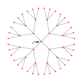
Figure 1: (Colour online) Cayley tree of order $k=3$.

The fixed vertex $x^{(0)}$ is called the 0th level and the vertices in $W_{n}$ are called the $n$th level. For the sake of simplicity, we put $|x|=d(x,x^{(0)}),x\in V$ [68].

Let us now define the neighborhoods that represent mutually competing interactions that we will use throughout the paper.

Definition 2.2

Hereafter, we use the following definitions for neighborhoods.

1. For $x,y\in V$, the vertices $x$ and $y$ are called nearest-neighbors (NN) if there exists an edge $\ell\in L$ connecting them, which is denoted by $\ell=\langle x,y\rangle$.

2. Two vertices $x,y\in V$ are called the next-nearest-neighbors (NNN) if there exists a vertex $z\in V$ such that $x,z$ and $y,z$ are NN, that is if $d(x,y)=2$.

3. The vertices $x$ and $y$ are called prolonged next-nearest-neighbors if $|x|\neq|y|$ and $d(x,y)=2$, and it is denoted by $\rangle x,y\langle$.

4. The next-nearest-neighbor vertices $x,y\in V$ that are not prolonged are called one-level next-nearest-neighbors if $|x|=|y|$ and are denoted by $\widetilde{\rangle x,y\langle}$.

5. For $x\in W_{n},y\in S(x)$, $z\in S(y)$ ($x\in W_{n},y\in W_{n+1}$, $z\in W_{n+2}$) and $n\in\mathbb{Z}_{+}$, the triple of vertices $x,y,z$ is called prolonged ternary next-nearest-neighbor (PTNNN) if there exist two adjacent edges $\ell_{1}=\langle x,y\rangle,\ell_{2}=\langle y,z\rangle\in L$ and is denoted by $\widetilde{\langle x,y,z\rangle}$.

6. Three vertices $x,y$ and $z$ are called a triple of neighbors if $\langle x,y\rangle$, $\langle y,z\rangle$ are nearest neighbors. They are denoted by $\langle x,y,z\rangle.$

2.2 Ising model

As stated in the introduction, the Ising model is a model introduced to explain the concept of ferromagnetism. The model can be derived from quantum mechanical considerations, by various conjectures and rough conclusions.

In 1925, Ising [69] incorrectly concluded that there is no phase transition in all dimensions. In 1936, Peierls [70] unexpectedly proved that the Lenz-Ising model undergoes a phase transition in 2 dimensions. Ising only solved the one-dimensional statistical problem and demonstrated that his model does not act like a ferromagnetic body [70]. There are several reasons why the Ising model has received great attention from physicists, mathematicians, and scientists working in other fields. Despite its simplicity, the Ising model is a usable and interesting model (see [71]).

As stated in the [72], Ising discussed only magnetic interpretation, but since his first definition in 1925, the same model has been applied to a number of other physical and biological systems such as gases, binary alloys, and cellular structures. A sociologically oriented application was proposed by Weidlich [73]. We give only one example here. Let us take the Hamiltonian

$$E_{\lambda}=-\sum_{i,j}I_{ij}\sigma_{i}\sigma_{j}-\mu H\sum_{i}\sigma_{i},$$ (2.1)

where $E_{\lambda}$ represents the total energy of a certain spin configuration $\lambda(\sigma_{l},\sigma_{2},\ldots,\sigma_{n})$ of $n$ magnets (where every $\sigma_{i}$ has a given value, $+1$ or $-1$) is assumed to depend on the external field $H$ and on spin-spin interaction parameters $I_{ij}$. In the simplest case, $I_{ij}$ is defined by

$$I_{ij}=\left\{\begin{array}[]{cc}I>0,&\text{for}\ (i,j)=\text{nearest\ neighbours\ in\ the lattice},\\ 0,&\text{otherwise}.\end{array}\right.$$

Considering the Hamiltonian (2.1), Weidlich [73] examined an application of the Ising model in sociology. Weidlich [73] considers a group of people. The state of each of these individuals is chosen to be either liberal (downward) or conservative (upward). Here, the total energy $E_{\lambda}$ is called the tension. The first expression in (2.1) is the tension arising from the interactions of people. The external field (the second expression) may be the liberal or conservative state of government. According to Weidlich [73], the tension is lowest when all people agree with each other and with the government. Of course, in such an application it may be necessary to ignore special neighborhoods and regular grid restrictions.

3 The dynamical behavior of the Ising model on a Cayley tree

In this section, we deal with the phase diagrams of dynamical systems associated with the Ising models corresponding to the Hamiltonians on a given Cayley tree with certain interactions. So far, this topic has been extensively studied due to the emergence of non-trivial magnetic orders (see [2, 3, 29, 30] and some references therein).

3.0.1 Vannimenus-Ising model with competing interactions on a Cayley tree

Let us consider the Hamiltonian

$$H(\sigma)=-{{J}_{p}}\sum\limits_{\rangle x,y\langle}{\sigma(x)\sigma(y)}-J\sum\limits_{\langle x,y\rangle}{\sigma(x)\sigma(y)},$$ (3.1)

where $\rangle x,y\langle$ represents the prolonged next nearest neighbor interaction and $\langle x,y\rangle$ represents the nearest neighbor interaction. We refer to this model as the Vannimenus-Ising model for short.

By considering the Hamiltonian (3.1), in addition to the paramagnetic and ferromagnetic phases in the drawn phase diagram, Vannimenus [2] also detected a new modulated phase, (see figure 3). In this section, we explain in detail how the phase diagrams of dynamical systems and phase variations are determined.

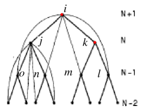
Figure 2: (Colour online) Four successive generations of a Cayley tree (two branches), with nearest-neighbor (heavy lines) and prolonged next-nearest neighbor (thin lines) interactions.

Vannimenus [2] considered a standard approach, which is to write down recursive equations relating the partition function of an $N$-generation tree to the partition functions of its subsystems with $(N-1)$ generations (see figure 2). To derive the recursive equations, he built the tree in the reverse direction, starting from its surface and moving towards its root. For a sufficiently large system, Vannimenus considered only the fastest growing terms.

For the partial partition functions $Z^{(N+1)}\left(\begin{smallmatrix}&i&\\ k&&j\end{smallmatrix}\right)$ there are a priori eight different partial partition functions $Z^{(N+1)}$, where $i,j,k\in\{-1,+1\}$. Therefore, one can obtain the following equation to derive the partial partition functions (see figure 2):

$$Z^{(N+1)}\left(\begin{array}[]{ccc}&i&\\ j&&k\end{array}\right) = \sum_{l,m,n,o\in\{-1,+1\}}\mathrm{e}^{[\beta Ji(k+j)+\beta J_{p}i(o+n+m+l)]}$$ (3.4)

$$\times Z^{(N)}\left(\begin{array}[]{ccc}&j&\\ o&&n\end{array}\right)Z^{(N)}\left(\begin{array}[]{ccc}&k&\\ m&&l\end{array}\right).$$ (3.9)

After simplifying, taking into account eight partial partition functions (3.4), Vannimenus [2] derived the following recursive equations:

$$\left\{\begin{array}[]{l}x^{(n+1)}=\frac{1}{a^{2}D}[(1+b^{2}x^{(n)})^{2}+(y_{1}^{(n)}+b^{2}y_{2}^{(n)})^{2}],\\ y_{1}^{(n+1)}=\frac{2}{D}[b^{2}y_{1}^{(n)}+y_{2}^{(n)}](x^{(n)}+b^{2}),\\ y_{2}^{(n+1)}=-\frac{2}{a^{2}D}[b^{2}y_{2}^{(n)}+y_{1}^{(n)}](x^{(n)}b^{2}+1),\end{array}\right.$$ (3.13)

where $D=\left(b^{2}+x^{(n)}\right)^{2}+\left(y_{2}^{(n)}+b^{2}y_{1}^{(n)}\right)^{2}$ and $a=\mathrm{e}^{J/T},b=\mathrm{e}^{J_{p}/T}.$
Furthermore, the average magnetization $m$ of the $N{\text{th}}$ generation is given by

$$m=\frac{2(y_{1}^{(n)}+y_{2}^{(n)})(x^{(n)}+1)}{(1+x^{(n)})^{2}+(y_{2}^{(n)}+y_{1}^{(n)}){}^{2}}.$$

3.1 How do we plot graphs of the phase diagrams of the Ising model?

A phase diagram of a dynamical system describes the structure of the phases, the stability of the phases, the transitions from one phase to another, and the corresponding transition lines [29, 30, 74]. In previous works [2, 6, 75], corresponding recurrence equations were analyzed using various computer codes, and thus the mathematical and physical interpretations of these systems of nonlinear equations were established. To run these programs, the phase diagrams were plotted using high performance computers. One examines the limit $(x^{(n)},\,\,y_{1}^{(n)},\,\,y_{2}^{(n)})\rightarrow(x^{*},\,\,y_{1}^{*},\,\,y_{2}^{*})$ as $n\rightarrow\infty$.

The recursive equations (3.13) give us (numerically) the phase diagram in $(T/J,-J_{p}/J)$-space. By obtaining the initial conditions (with $y_{1}^{(1)},\,\,y_{2}^{(1)}\neq 0$), we obtain the next terms in the recurrence equations (3.13), so that we can observe the behavior of these equations by performing a large number of iterations. As a result of these iterations, we try to reach the fixed points $(x^{*},\,\,y_{1}^{*},\,\,y_{2}^{*})$ of these iterative equations. Then, taking this fixed point as new initial data, one can construct a phase (or Gibbs measure) that corresponds to a paramagnetic phase if $y_{1}^{*}=0,\,\,y_{2}^{*}=0$ or to a ferromagnetic phase if $y_{1}^{*},\,\,y_{2}^{*}\neq 0.$ Secondly, the system may be periodic with period $p$ and taking into account the sequence $(x^{(k)},\,\,y_{1}^{(k)},\,\,y_{2}^{(k)})$ with $k=0,\,\,1,\,\,\ldots,\,\,p-1$ as new initial data, one can construct a phase. Here, the case $p=2$ corresponds to the antiferromagnetic phase and the case $p=4$ corresponds to the so-called antiphase, denoted for compactness by $\left\langle 2\right\rangle$. It corresponds to an appropriate phase with a given period. Finally, the system can remain aperiodic, which is associated to an incommensurable phase. It is difficult to numerically distinguish between a non-periodic state and a state with a very long period (see [2, 6, 29, 30, 74, 75] for details).

If these iterations are based on the resulting values and $\lim\limits_{n\rightarrow\infty}x^{(n)}\neq 0,\,\,\lim\limits_{n\rightarrow\infty}y_{1}^{(n)}=0,\lim\limits_{n\rightarrow\infty}y_{2}^{(n)}=0$, then the diagram shows a paramagnetic phase region (shortly, P) (high symmetric phase). If at least one of the limits $\lim\limits_{n\rightarrow\infty}y_{1}^{(n)}$ and $\lim\limits_{n\rightarrow\infty}y_{2}^{(n)}$ is non-zero, then the relevant phase corresponds to the ferromagnetic (F) region in our phase diagram. Otherwise, if there are no limit values, i.e., after a certain iteration, the terms of the index are not always the same, then the terms of these sequences will either change periodically or randomly. In such cases, for example, if the terms after 100000 terms are the same as the two periods, then we have expressed this region with period 2, briefly P2. If it is 3 periods, then we have expressed the region with period 3, briefly P3. Thus, we have termed the modulated phase (M) in the phase regions in the other case, which is called the periodic phase, up to period 12 (P12).

Let us consider the equation

$$\lim_{n\rightarrow\infty}(x^{(n)},y_{1}^{(n)},y_{2}^{(n)})=\lim_{n\rightarrow\infty}(x^{(n+p)},y_{1}^{(n+p)},y_{2}^{(n+p)})=(x^{(*)},y_{1}^{(*)},y_{2}^{(*)}).$$ (3.14)

The nonnegative integer $p$ is called the period of convergent sequence $(x^{(n)},y_{1}^{(n)},y_{2}^{(n)})$. For simplicity, let $F^{(n)}=(x^{(n)},y_{1}^{(n)},y_{2}^{(n)})$.

To illustrate this process graphically, we have expressed each phase with distinct colours. We have fixed the corresponding colouring of the phase diagrams in table 1.

Table 1: (Colour online) The colours of the phase diagrams.

Periodic point	colour	Kind of Phases
$F^{(n)}\rightarrow(x^{*},0,0)$	White	“PARAMAGNETIC"
$F^{(n)}\rightarrow(x^{*},y_{1}^{*},y_{2}^{*})$	Red	“FERROMAGNETIC"
	Mangotango	“PARAMODULATED"
$\left.\begin{array}[]{l}F^{(n)}\\ F^{(n+2)}\end{array}\right\}\rightarrow(x^{(*)},y_{1}^{(*)},y_{2}^{(*)})$	Yellow	“PERIOD 2"
$\left.\begin{array}[]{l}F^{(n)}\\ F^{(n+3)}\end{array}\right\}\rightarrow(x^{(*)},y_{1}^{(*)},y_{2}^{(*)})$	Lime	“PERIOD 3"
$\left.\begin{array}[]{l}F^{(n)}\\ F^{(n+4)}\end{array}\right\}\rightarrow(x^{(*)},y_{1}^{(*)},y_{2}^{(*)})$	Aqua	“PERIOD 4"
$\left.\begin{array}[]{l}F^{(n)}\\ F^{(n+5)}\end{array}\right\}\rightarrow(x^{(*)},y_{1}^{(*)},y_{2}^{(*)})$	Blue	“PERIOD 5"
$\left.\begin{array}[]{l}F^{(n)}\\ F^{(n+6)}\end{array}\right\}\rightarrow(x^{(*)},y_{1}^{(*)},y_{2}^{(*)})$	Fuchsia	“PERIOD 6"
$\left.\begin{array}[]{l}F^{(n)}\\ F^{(n+7)}\end{array}\right\}\rightarrow(x^{(*)},y_{1}^{(*)},y_{2}^{(*)})$	3DDkShadow	“PERIOD 7"
$\left.\begin{array}[]{l}F^{(n)}\\ F^{(n+8)}\end{array}\right\}\rightarrow(x^{(*)},y_{1}^{(*)},y_{2}^{(*)})$	Maroon	“PERIOD 8"
$\left.\begin{array}[]{l}F^{(n)}\\ F^{(n+9)}\end{array}\right\}\rightarrow(x^{(*)},y_{1}^{(*)},y_{2}^{(*)})$	Green	“PERIOD 9"
$\left.\begin{array}[]{l}F^{(n)}\\ F^{(n+10)}\end{array}\right\}\rightarrow(x^{(*)},y_{1}^{(*)},y_{2}^{(*)})$	Olive	“PERIOD 10"
$\left.\begin{array}[]{l}F^{(n)}\\ F^{(n+11)}\end{array}\right\}\rightarrow(x^{(*)},y_{1}^{(*)},y_{2}^{(*)})$	Teal	“PERIOD 11"
$\left.\begin{array}[]{l}F^{(n)}\\ F^{(n+p)}\end{array}\right\}\rightarrow(x^{(*)},y_{1}^{(*)},y_{2}^{(*)})$	Purple ($p>11$)	“MODULATED"

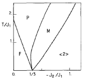
Figure 3: The phase diagram of Vannimenus model on the rectangular region $[0,1.3]\times[0,2.3]$ (see [2]).

In [16], the generalization of the Vannimenus’s study on a Cayley tree of arbitrary order was introduced. In these works, the phase diagrams of two of the simplest Ising models were examined in detail. The phase diagram in [2] was plotted for the first region only. In the study by Vannimenus, the phase diagram was investigated. The phase diagram of the same model was first tried in Visual Basic, then $C^{++}$ and later Delphi programming languages. The best result was obtained with the code written in Delphi programming language (see figure 4).

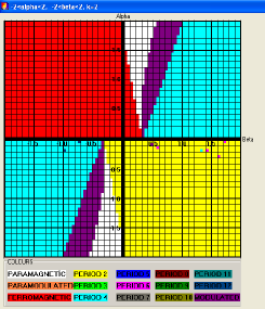
Figure 4: (Colour online) The phase diagram of Vannimenus model on the rectangular region $[-2,2]\times[-2,2]$ (see [37]).

Vannimenus [2] studied the Ising model in conjunction with the Hamiltonian (3.1) on the Cayley tree of the order two. In figure 3 plotted by Vannimenus [2], the phase diagram of the dynamical system corresponding to the Ising model with competing interactions includes ferromagnetic (F), paramagnetic (P), modulated (M), and periodic (+ + – –) structure ($\left\langle 2\right\rangle$, in short). Considering the same Hamiltonian, we analyzed the phase diagrams associated with the Ising model on a Cayley tree of arbitrary order [6]. We accurately plotted the phase diagrams [6]. We characterized the phases by the sequence of stable points of the recursion relations. We examined the effect of the order of the Cayley tree on the phase diagrams [6, 46].

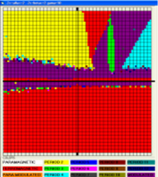
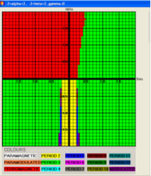
Figure 5: (Colour online) The phase diagrams on the rectangular region $[-2,2]\times[-2,2]$ of some given Ising models.

Looking at the phase diagram to the right of figure 5, the image quality obtained is better than that on the left of figure 5. The phase diagram was drawn using the $C^{++}$ programming language on the left. The figure on the right was drawn using the Delphi Programming language. In addition, the mean magnetization equations for each level of the above-mentioned Ising and Potts models were derived [2, 76].

Remark 3.1

It should be noted that we have used Vannimenus’ approach to plot phase diagrams.

3.2 The phase diagrams of Ising model with NN and PTNNN interactions

In this subsection, for convenience we consider one of the simplest Ising models (see [38, 46]). Note that this subsection is based on [46].

Let us consider the following Hamiltonian

$$H(\sigma)=-{{J}_{{{t}_{p}}}}\sum\limits_{{\mathop{\rangle x,y,z\langle}}\,}{}\sigma(x)\sigma(y)\sigma(z)-{{J}_{1}}\sum\limits_{\langle x,y\rangle}\sigma(x)\sigma(y),$$ (3.15)

where $\mathop{\rangle x,y,z\langle}$ represents competing prolonged ternary next nearest-neighbor (PTNNN) and $\langle x,y\rangle$ represents competing nearest-neighbor (NN), where ${{J}_{{{t}_{p}}}},{{J}_{1}}\in\mathbb{R}$ are coupling constants.

Here, we analyze the dynamical behavior and the phase diagram of the Ising model corresponding to the Hamiltonian (3.15). We investigate the relationship between the partition function on $V_{n}$ and the partition function on subsets of $V_{n-1}$ to obtain the recurrent equations. The recurrence equations show how their impact propagates along the tree for a given initial condition on $V_{1}$.
Let

$$\sigma_{S}^{+}(x^{(0)})=\left(\begin{matrix}\sigma({{y}_{k}}),\cdots,\sigma({{y}_{2}}),\sigma({{y}_{1}})\\ +\\ \end{matrix}\right),$$

be a configuration in $\{-1,+1\}^{B_{1}(x^{(0)})}$ (see figure 6), where $B_{1}(x^{(0)})=\{y\in S(x^{(0)})\}\cup\{x^{(0)}\}$.
Let $m$ represent the number of spins down ($\sigma(y_{i})=-1$) at the first level $W_{1}$, where $0\leqslant m\leqslant k$. Then, at the first level $W_{1}$, $(k-m)$ is the number of spins up ($\sigma(y_{i})=+1$).

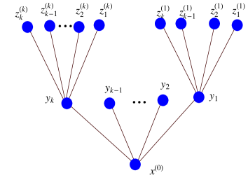
Figure 6: (Colour online) Two generations of arbitrary order $k>1$ semi-infinite Cayley tree $\Gamma^{k}$ (branching ratio is finite $k$).

In figure 6, the root of the lattice that emanates $k$ edges of $\Gamma^{k}$ is a fixed vertex $x^{(0)}$, therefore $y_{j}\in S(x^{(0)}),\,\,z_{i}^{(j)}\in S(y_{j})$. Denote a configuration in $\{-1,+1\}^{B_{1}(y_{i})}$ by

$$\sigma_{S}^{+}(y_{i})=\left(\begin{matrix}\sigma(z_{k}^{(i)}),\cdots,\sigma(z_{2}^{(i)}),\sigma(z_{1}^{(i)})\\ +\\ \end{matrix}\right).$$

Let the $m$ spins on $\{-1,+1\}^{B_{1}(S(y_{i}))}$ (the second level $W_{2}$) be spins down, i. e., $\sigma(z_{j}^{(i)})=-1$, where $0\leqslant m\leqslant k.$ Let the remaining number of $(k-m)$ of them be spin up i. e., $\sigma(z_{j}^{(i)})=+1$. Let

$$\sigma_{S}^{-}(x^{(0)})=\left(\begin{matrix}\sigma({{y}_{k}}),\ldots,\sigma({{y}_{2}}),\sigma({{y}_{1}})\\ -\\ \end{matrix}\right),$$

be a configuration in $\{-1,+1\}^{S(x^{(0)})}$. Let $m$ be the number of spins down, i. e., $\sigma(y_{i})=-1$ at the first level ${{W}_{1}}$, where $0\leqslant m\leqslant k.$ Considering the vertices in the subsets $W_{1}$ and $W_{2}$ of the graph $\Gamma^{k}$, we can similarly construct the following configuration. Let

$$\sigma_{S}^{-}({{y}_{i}})=\left(\begin{matrix}\sigma(z_{k}^{(i)}),\cdots,\sigma(z_{2}^{(i)}),\sigma(z_{1}^{(i)})\\ -\\ \end{matrix}\right),$$

be a configuration in $\{-1,+1\}^{B_{1}(y_{i})}$ (see figure 6). Let $m$ be the number of spins down $\sigma(z_{j}^{(i)})=-1$ at the second level ${{W}_{2}}$, where $0\leqslant m\leqslant k.$

For clarity, denote the configuration of the set $\Phi^{B_{1}(x^{(0)})}$ by

$$S_{m}^{(k-m)}(\sigma({{x}^{(0)}}))=\left(\begin{matrix}\overbrace{++\cdots+}^{k-m}\overbrace{--\cdots-}^{m}\\ \sigma(x^{(0)})\\ \end{matrix}\right).$$

Let

$${{Z}^{(n)}}\left(\begin{matrix}{{i}_{1}},{{i}_{2}},\ldots,{{i}_{k}}\\ {{i}_{0}}\\ \end{matrix}\right)={{Z}^{n}}=\sum\limits_{{\sigma_{n}}\in{{\Omega}^{{{V}_{n}}}}}{\exp(-\beta H({{\sigma}_{n}}))},$$

be the partition function on ${{V}_{n}}$, where the spin in the root $x^{(0)}$ is ${{i}_{0}}$ and the $k$ spins in the proceeding ones are ${{i}_{1}},{{i}_{2}},\ldots,{{i}_{k}}$. A priori, there are $2^{k+1}$ partition functions $Z^{(n)}$. However, it is plausible to assume that the different branches are comparable.

To make the paper more readable, we use shorter notations, as shown below. As a result, we can show that there are only four independent variables, namely

$${{z}_{1}}={{Z}^{(n)}}\left(\begin{matrix}+,+,\ldots,+\\ +\\ \end{matrix}\right),\quad{{z}_{2}}={{Z}^{(n)}}\left(\begin{matrix}-,-,\ldots,-\\ +\\ \end{matrix}\right),$$

$${{z}_{3}}={{Z}^{(n)}}\left(\begin{matrix}+,+,\ldots,+\\ -\\ \end{matrix}\right),\quad{{z}_{4}}={{Z}^{(n)}}\left(\begin{matrix}-,-,\ldots,-\\ -\\ \end{matrix}\right).$$

Then, arbitrary partial partition function ${{Z}^{(n)}}\left(\begin{matrix}{{i}_{1}},{{i}_{2}},\ldots,{{i}_{k}}\\ {{i}_{0}}\\ \end{matrix}\right)$ is a combination of ${{z}_{1}},{{z}_{2}},{{z}_{3}},{{z}_{4}}$. For instance, for $\sigma({{i}_{0}})=+$, the partial partition function can be written by

$${{Z}^{(n)}}\left(\begin{matrix}{{i}_{1}},{{i}_{2}},\ldots,{{i}_{k}}\\ +\\ \end{matrix}\right)=\left(\begin{matrix}\overbrace{++\ldots+}^{k-m}\overbrace{--\cdots-}^{m}\\ +\\ \end{matrix}\right)=z_{1}^{\frac{m}{k}}z_{2}^{\frac{k-m}{k}},$$

where $m$ is the number of spins down on ${{W}_{1}}.$ Similarly, for $\sigma({{i}_{0}})=-1$, the partial partition function can be written by

$${{Z}^{(n)}}\left(\begin{matrix}{{i}_{1}},{{i}_{2}},\ldots,{{i}_{k}}\\ -\\ \end{matrix}\right)=\left(\begin{matrix}\overbrace{++\cdots+}^{k-m}\overbrace{--\cdots-}^{m}\\ -\\ \end{matrix}\right)=z_{3}^{\frac{m}{k}}z_{4}^{\frac{k-m}{k}}.$$

By adjusting the variables ${{u}_{i}}=\sqrt[k]{z_{i}}$, one gets

$$\left\{\begin{array}[]{l}u_{1}^{{}^{\prime}}=a\left(bu_{1}+b^{-1}u_{2}\right)^{k},\\ u_{2}^{{}^{\prime}}=a^{-1}\left(b^{-1}u_{3}+bu_{4}\right)^{k},\\ u_{3}^{{}^{\prime}}=a^{-1}\left(b^{-1}u_{1}+bu_{2}\right)^{k},\\ u_{4}^{{}^{\prime}}=a\left(bu_{3}+b^{-1}u_{4}\right)^{k},\end{array}\right.$$

where $a=\mathrm{e}^{J_{1}/T}$, $b=\mathrm{e}^{J_{t_{p}}}/T)$ and the variables $u_{i}^{{}^{\prime}}$ represent the ${{Z}^{(n+1)}}$.

Using the partial partition functions $u_{i}$, we obtain the total partition function in the form;

$$Z^{(n)}=(u_{1}+u_{2})^{k}+(u_{3}+u_{4})^{k}.$$

To plot the phase diagrams, we consider the following reduced variables

$$\left\{\begin{array}[]{l}x=\frac{u_{2}+u_{3}}{u_{1}+u_{4}},\\ y_{1}=\frac{u_{1}-u_{4}}{u_{1}+u_{4}},\\ y_{2}=\frac{u_{2}-u_{3}}{u_{1}+u_{4}}.\end{array}\right.$$ (3.16)

The variable $x$ in the system (3.16) is simply a measure of the frustration of nearest-neighbor bonds, not an order parameter like $y_{1},y_{2}$ (see [2] for details). By substituting the variables in the equation (3.16) as follows:

$$u_{1}=\frac{(1+y_{1})A}{2},\quad u_{2}=\frac{(x+y_{2})A}{2},\quad u_{3}=\frac{(x-y_{2})A}{2},\quad u_{4}=\frac{(1-y_{1})A}{2},$$

where $A=u_{1}+u_{4}$, and if we replace the variables $u_{i}^{{}^{\prime}}$ in the system (3.16), we derive the recurrence equations:

$$\left\{\begin{array}[]{l}{{x}^{{}^{\prime}}}=\frac{1}{{{a}^{2}}D}[(x-{{y}_{2}}+{{b}^{2}}(1-{{y}_{1}}{{))}^{k}}+{{(1+{{y}_{1}}+{{b}^{2}}(x+{{y}_{2}}))}^{k}}],\\ y_{1}^{{}^{\prime}}=\frac{1}{D}[({{b}^{2}}(1+{{y}_{1}})+x+{{y}_{2}}{{)}^{k}}-{{({{b}^{2}}(x-{{y}_{2}})+1-{{y}_{1}})}^{k}}],\\ y_{2}^{{}^{\prime}}=\frac{1}{{{a}^{2}}D}[(x-{{y}_{2}}+{{b}^{2}}(1-{{y}_{1}}{{))}^{k}}-{{(1+{{y}_{1}}+{{b}^{2}}(x+{{y}_{2}}))}^{k}}],\end{array}\right.$$ (3.17)

where $D=\left(x+y_{2}+b^{2}(1+y_{1})\right)^{k}+\left(b^{2}(x-y_{2})+1-y_{1}\right)^{k}.$
For the sake of completeness we restate the method studied in [2, 68]. With a suitable computer code, we calculate the consecutive terms of the recurrence equations (3.17) numerically, taking into account the rules given in table 1. Thus, with this method, we plot the phase diagram corresponding to the recursive relations (3.17) in the space $(-{{J}_{{{t}_{p}}}}/{{J}_{1}},T/{{J}_{1}})$. Assume $(-{{J}_{{{t}_{p}}}}/{{J}_{1}})=\beta$, $T/{{J}_{1}}=\alpha$ and respectively $b=\exp(-{{\alpha}^{-1}}\beta)$, $a=\exp({{\alpha}^{-1}})$.

By substituting the initial conditions

$$\left\{\begin{array}[]{l}{{x}^{(1)}}=\frac{{{b}^{2k}}+{{a}^{2k}}}{a((ab{{)}^{2k}}+1)},\\ y_{1}^{(1)}=\frac{{{(ab)}^{2k}}-1}{{{(ab)}^{2k}}+1},\\ y_{2}^{(1)}=\frac{{{b}^{2k}}-{{a}^{2k}}}{{{a}^{2}}((ab{{)}^{2k}}+1)},\end{array}\right.$$

under boundary condition $\bar{\sigma}^{(n)}(V\backslash V_{n})\equiv 1$ in the recursive equations (3.17), we obtain the second and third terms, respectively, so we run the computer code and numerically calculate the terms after the $n$th term of this sequence for natural number $n$ large enough (see [2, 46, 77] for details).

In the simplest sense, as explained earlier, a fixed point $({{x}^{*}},y_{1}^{*},y_{2}^{*})$ is obtained. In other words, for sufficiently large natural number $n$, the other terms of this sequence are equal or become equal after a certain period. For each binary value $(-J_{{t}_{p}}/J_{1},T/J_{1})\in[-2,2]\times[-2,2]$ selected in the two-dimensional plane, we obtain a fixed point $y_{1}^{*}=0,y_{2}^{*}=0$, then kind of the phase becomes paramagnetic phase and point $(-J_{{t}_{p}}/J_{1},T/J_{1})$ is marked with white or we obtain a ferromagnetic phase if $y_{1}^{*},y_{2}^{*}\neq 0$ taking into account the average magnetization equation.

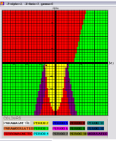
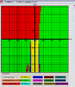
Figure 7: (Colour online) Relevant phase diagrams of the model (3.15) for $k=2$ (left-hand figure) and $4$ (right-hand figure), respectively (see [46]).

Figures in 7 illustrate the resulting phase diagrams for various values of $k$. The phase diagram for $J_{1}>0$ and $k=2$ incorporates a ferromagnetic phase and a novel phase with period $3$ (see [38, 46]). The phase diagram of the recursive system in (3.17) contains interesting images for competing interactions $(J_{1}<0)$. The phase diagram in this case is extremely detailed, with at least four multicritical Lifshitz points, two of which are at zero temperature and the other two at nonzero temperature. The key novelty is the existence of multicritical Lifshitz points that are not at zero temperature, as opposed to zero temperature in prior publications by Vannimenus [2] and Mariz [3]. It is worth noting that the paramagnetic phase has vanished in this situation. The role of $k$ is clearly apparent on the phase diagrams.

Note that the recurrence equations (3.17) and phase diagrams in this subsection are based on the work [46].

3.3 Variation of wave-vectors

Here, we examine in detail the variation of the wave vector with temperature in the modulated phase region. The variation of the wave vector shows narrow commensurate in the incommensurate regions [62]. An incommensurate structure with a given wave-vector is represented by a fixed defect concentration [5]. Furthermore, the wave-vector of the modulated structure (i.e. the defect concentration) varies continuously with piecewise constant parts at each commensurate value (the resulting curve is called a devil’s staircase) [5].

In this subsection, we study the behavior of the average magnetization in a period or the dynamical magnetization as a function of the reduced temperature. This investigation allows us to characterize the nature of the transition. The average magnetization $m$ associated with the model (3.15) for the $n$th generation is given by

$$m = \frac{Z_{+}^{(n)}-Z_{-}^{(n)}}{Z_{+}^{(n)}+Z_{-}^{(n)}}=\frac{\sum\limits_{i_{0},i_{1},\ldots,i_{k}\in\{-1,1\}}{i_{0}{{Z}^{(n)}}\left(\begin{matrix}{{i}_{1}},{{i}_{2}},\cdots,{{i}_{k}}\\ i_{0}\\ \end{matrix}\right)}}{\sum\limits_{i_{0},i_{1},\ldots,i_{k}\in\{-1,1\}}{{{Z}^{(n)}}\left(\begin{matrix}{{i}_{1}},{{i}_{2}},\cdots,{{i}_{k}}\\ i_{0}\\ \end{matrix}\right)}}$$ (3.18)

$$= \frac{{{(1+x+{{y}_{1}}+{{y}_{2}})}^{k}}-{{(1+x-{{y}_{1}}-{{y}_{2}})}^{k}}}{{{(1+x+{{y}_{1}}+{{y}_{2}})}^{k}}+{{(1+x-{{y}_{1}}-{{y}_{2}})}^{k}}}$$

and we obtain the magnetization of the root $x^{(0)}$ as

$$\left\langle{{\sigma}_{0}}\right\rangle=\underset{n\to\infty}{\mathop{\lim}}\,\frac{Z_{+}^{(n)}-Z_{-}^{(n)}}{Z_{+}^{(n)}+Z_{-}^{(n)}}.$$

Here, by using numerical calculations we investigate the behavior of the system given in (3.17). Finally, we investigate how the wave-vector changes with temperature. A numerically convenient definition of the wave-vector is

$$q=\underset{N\to\infty}{\mathop{\lim}}\,\left(\frac{1}{2}\frac{n}{N}\right),$$

where $n$ is the number of times that the magnetization (3.18) changes the sign during $N$ successive iterations [2].

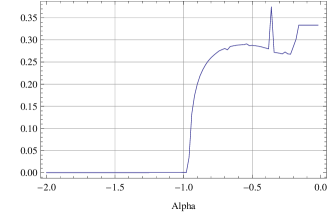
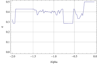
Figure 8: (Colour online) Change of the wave-vectors for $\beta=0.466$, $k=2$ (left-hand) and $\beta=-0.23$, $k=4$ (right-hand) (see [46]).

The magnetization wave-vector varies continuously with the temperature and the order of the Cayley tree. Figure 8 shows typical graphs of $q$ versus $T$. In figure 7, for $k=2$, the point $(\beta,\alpha)=(-0.45,-0.15)$ is the multicritical Lifshits point. The graphs of $q$ versus $T/{{J}_{1}}$ are changing very fast around $(-1.25,0)$. In figure 7, for $k=4$ in the fourth region, there is a modulated phase and the island-shaped region is quite narrow. The analysis of such general phase diagrams is quite complicated. Therefore, the Lyapunov exponents must be examined in detail. Moreover, for a more detailed study of variation of the wave-vector $q$ versus $T/{{J}_{1}}$, we need to find the main locking steps that should be present in accordance with the general theory given by Vannimenus [2].

In figures 8, we describe the variation of wave-vectors for some values of interactions in the Ising model, which is determined by the Hamiltonian given in (3.15). As an important result in our phase diagrams, if the Hamiltonian is added to the next nearest neighbor with the triple prolonged (PNNN), the paramagnetic regions disappear at low temperatures [38, 46]. In the phase diagram obtained by Vannimenus, Lifshitz points called “multi-critical points” are obtained at zero temperatures. However, in our new phase diagrams, Lifshitz points appear at non-zero temperatures. We first plotted the phase diagrams corresponding to the Ising system of triple interaction on a two-stage Cayley tree [68]. These phase diagrams obtained are much richer compared to the previous ones, and the Lifshitz points have more different characteristics. In [62], the authors plotted the phase diagrams of Ising model determined by Hamiltonian on a Cayley tree of arbitrary order, and thus the wave-vectors for some values were drawn. The Ising models with three interactions have been tested to examine the variation of wave-vectors and to plot them in three parameters. Two-dimensional graphs have been successfully drawn for some constants of one of these parameters. In [46], for particular values of the coupling constants and $T$, we have plotted the magnetization graphs of the nonlinear-dynamical system.

3.4 The study of the Lyapunov exponent

As stated in [46], the stability analysis for the ferromagnetic phase is more difficult than that of the paramagnetic phase because the fixed point is not the same for the whole phase. The Lyapunov exponent for the models associated to the given Hamiltonians was calculated numerically (see [6]). In addition, we demonstrated that every region of negative $\lambda$ corresponds to the stability domain of a given cycle [6]. Since the intervals are very narrow, the description of the distinction between long-periodic cycles (commensurate or incommensurate phases) and calculations are difficult to perform. The answer to our problem consists of nonlinear analysis techniques such as Lyapunov exponents corresponding to the trajectory of the dynamical system [6, 46].

The positive values of Lyapunov exponents show the chaotic structures of the phases [78]. In other words, the Lyapunov exponents of the map show the presence of chaotic structures, associated with a strange attractor [79]. Moreover, Lyapunov exponents support the existence of a region of chaotic phases, associated with a strange attractor of the map [79]. Vannimenus [2] has numerically shown that the error bars indicate the fluctuations in the last hundred out of 10 000 iteration steps. Lyapunov exponents measure the mean exponential rate of convergence or divergence of trajectories surrounding the attractors. By ensuring the accuracy of the graphics obtained for the Lyapunov exponents of the works in the literature, the Lyapunov exponents of the new models were drawn [6, 46]. Pasquini et al. [80] have characterized the formal expression of the Lyapunov exponents via the convergence of the map towards a fixed point before performing the thermodynamic limit, in a restricted ensemble of disorder realizations. Furthermore, Pasquini et al. [80] determined the analytic upper and lower bounds for the Lyapunov exponents of the product of random matrices in the one-dimensional disordered Ising model.

Let us consider a one-dimensional map $f:\mathbb{R}\rightarrow\mathbb{R}$. Let $x,x+\delta\in\mathbb{R}$. Under the first iteration of the function $f$, if the distance between $f(x)$ and $f(x+\delta)$ changes exponentially, then we have

$$d(f(x),f(x+\delta))=\mathrm{e}^{\lambda}d(x,x+\delta).$$

After $n$th iteration, one gets

$$d(f^{n}(x),f^{n}(x+\delta))=\mathrm{e}^{n\lambda}d(x,x+\delta).$$ (3.19)

From (3.19), we have

$$\lambda=\frac{1}{n}\ln\left(\frac{d(f^{n}(x),f^{n}(x+\delta))}{\delta}\right).$$

If the limit

$$\lambda=\lim_{n\rightarrow\infty}\frac{1}{n}\ln\left(\frac{d(f^{n}(x),f^{n}(x+\delta))}{\delta}\right)$$

exists as $\delta\rightarrow 0$, the quantity $\lambda$ is called Lyapunov exponent of the function $f$.

In [6, 46], we were able to establish a formal expression of the Lyapunov exponents in terms of the approach by Vannimenus [2].

Definition 3.1

Consider a differentiable vector-valued function

$$\mathbf{F}(\mathbf{x})=({{F}_{1}}(\mathbf{x})....{{F}_{n}}(\mathbf{x})),$$

where $\mathbf{F}:{{\mathbb{R}}^{m}}\to{{\mathbb{R}}^{n}}$ and ${{F}_{i}}:{{\mathbb{R}}^{m}}\to{{\mathbb{R}}}$. The Jacobian matrix of $\mathbf{F}$ is a $n\times m$ matrix:

$$\mathbf{DF}\equiv\frac{\mathrm{d}\mathbf{F}}{\mathrm{d}\mathbf{x}}=\left(\begin{matrix}\frac{\mathrm{d}{{F}_{1}}}{\mathrm{d}{{x}_{1}}}&\cdots&\frac{\mathrm{d}{{F}_{1}}}{\mathrm{d}{{x}_{m}}}\\ \vdots&\vdots&\vdots\\ \frac{\mathrm{d}{{F}_{n}}}{\mathrm{d}{{x}_{1}}}&\cdots&\frac{\mathrm{d}{{F}_{n}}}{\mathrm{d}{{x}_{m}}}\\ \end{matrix}\right).$$ (3.20)

In this subsection, in order to illustrate the stability of the fixed point $({{x}^{*}},0,0)$, we consider the following Hamiltonian (see [6]):

$$H(\sigma)=-{{J}_{{{t}_{p}}}}\sum\limits_{\overset{}{\mathop{>x,y,z<}}\,}{}\sigma(x)\sigma(y)\sigma(z)-{{J}_{p}}\sum\limits_{>x,y<}{\sigma(x)\sigma(y)}-{{J}_{1}}\sum\limits_{<x,y>}{}\sigma(x)\sigma(y),$$ (3.21)

where the first sum encompasses all prolonged ternary next-nearest neighbors, the second sum encompasses all prolonged next-nearest neighbors, and the third sum encompasses all nearest neighbors, and $J_{t_{p}},J_{p},J_{1}\in\mathbb{R}$ are coupling constants.

Obviously, if $k=2$ and $J_{t_{p}}=0$, the Hamiltonian (3.21) will be the same as the Hamiltonian discussed by Vannimenus [2]. In the case ${{J}_{{{t}_{p}}}}\times J_{1}\neq 0$ and ${{J}_{p}}=0$, the model has been investigated by Akın et al. [46].

In [6], we derived the recurrent equations associated to the Hamiltonian (3.21) with ${{J}_{{{t}_{p}}}}\times J_{1}\times{{J}_{p}}\neq 0$ as follows. For convenience, we assume

$$x_{n+1} = \frac{(b^{2}(x_{n}-z_{n})+c^{2}(1-y_{n}))^{k}+(1+y_{n}+b^{2}c^{2}(x_{n}+z_{n}))^{k}}{a^{2}\left((b^{2}c^{2}(1+y_{n})+x_{n}+z_{n})^{k}+(c^{2}(x_{n}-z_{n})+b^{2}(1-y_{n}))^{k}\right)},$$ (3.22)

$$y_{n+1} = \frac{2((b^{2}c^{2}(1+y_{n})+x_{n}+z_{n})^{k}-(c^{2}(x_{n}-z_{n})+b^{2}(1-y_{n}))^{k})}{(b^{2}c^{2}(1+y_{n})+x_{n}+z_{n})^{k}+(c^{2}(x_{n}-z_{n})+b^{2}(1-y_{n}))^{k}},$$ (3.23)

$$z_{n+1} = \frac{((b^{2}(x_{n}-z_{n})+c^{2}(1-y_{n}))^{k}-(1+y_{n}+b^{2}c^{2}(x_{n}+z_{n}))^{k})}{a^{2}\left((b^{2}c^{2}(1+y_{n})+x_{n}+z_{n})^{k}+(c^{2}(x_{n}-z_{n})+b^{2}(1-y_{n}))^{k}\right)},$$ (3.24)

where $a=\mathrm{e}^{(J_{1}/T)}$, $b=\mathrm{e}^{(J_{p}/T)}$, $c=\mathrm{e}^{(J_{t_{p}}/T)}$, $x_{n+1}=F_{1}(x_{n},y_{n},z_{n})$, $y_{n+1}=F_{2}(x_{n},y_{n},z_{n})$ and $z_{n+1}=F_{3}(x_{n},y_{n},z_{n})$ (see [6] for details).

Linearizing the iterative equations (3.22)–(3.24) around the subsequent points of the trajectory yields linear iterative equations for the perturbations. The Lyapunov exponents can be calculated in the following way.
Let us consider the operator $\mathbf{F}:{{\mathbb{R}}^{3}}\to{{\mathbb{R}}^{3}}$ defined by

$$\mathbf{F}(x_{n+1},y_{n+1},z_{n+1})=[{{F}_{1}}({{x}_{n}},{{y}_{n}},{{z}_{n}}),{{F}_{2}}({{x}_{n}},{{y}_{n}},{{z}_{n}}),{{F}_{3}}({{x}_{n}},{{y}_{n}},{{z}_{n}})].$$ (3.25)

Now, we linearize the operator (3.25) around the successive points of the trajectory $(x_{1},y_{1},z_{1})$,…, $(x_{k},y_{k},z_{k})$ satisfying the recurrence equations for the perturbations $(\delta x_{n},\delta y_{n},\delta z_{n})$.

From the definition of differentiability in multivariable calculus, we have

$$x_{n{+}1}{-}F_{1}(x_{k},y_{k},z_{k}) = \frac{\partial F_{1}(x_{n},y_{n},z_{n})}{\partial x_{n}}(x_{n}-x_{k})+\frac{\partial F_{1}(x_{n},y_{n},z_{n})}{\partial y_{n}}(y_{n}-y_{k}){+}\frac{\partial F_{1}(x_{n},y_{n},z_{n})}{\partial z_{n}}(z_{n}-z_{k}),$$

$${{y}_{n{+}1}}{-}{{F}_{2}}({{x}_{k}},{{y}_{k}},{{z}_{k}}) = \frac{\partial{{F}_{2}}({{x}_{n}},{{y}_{n}},{{z}_{n}})}{\partial{{x}_{n}}}({{x}_{n}}{-}{{x}_{k}})+\frac{\partial{{F}_{2}}({{x}_{n}},{{y}_{n}},{{z}_{n}})}{\partial{{y}_{n}}}({{y}_{n}}{-}{{y}_{k}})+\frac{\partial{{F}_{2}}({{x}_{n}},{{y}_{n}},{{z}_{n}})}{\partial{{z}_{n}}}({{z}_{n}}{-}{{z}_{k}}),$$

$${{z}_{n+1}}{-}{{F}_{3}}({{x}_{k}},{{y}_{k}},{{z}_{k}}) = \frac{\partial{{F}_{3}}({{x}_{n}},{{y}_{n}},{{z}_{n}})}{\partial{{x}_{n}}}({{x}_{n}}{-}{{x}_{k}})+\frac{\partial{{F}_{3}}({{x}_{n}},{{y}_{n}},{{z}_{n}})}{\partial{{y}_{n}}}({{y}_{n}}{-}{{y}_{k}})+\frac{\partial{{F}_{3}}({{x}_{n}},{{y}_{n}},{{z}_{n}})}{\partial{{z}_{n}}}({{z}_{n}}{-}{{z}_{k}}).$$

We obtain the Jacobian matrix as follows:

$$L_{n}=\left(\begin{matrix}\frac{\partial{{F}_{1}}({{x}_{n}},{{y}_{n}},{{z}_{n}})}{\partial{{x}_{n}}}&\frac{\partial{{F}_{1}}({{x}_{n}},{{y}_{n}},{{z}_{n}})}{\partial{{y}_{n}}}&\frac{\partial{{F}_{1}}({{x}_{n}},{{y}_{n}},{{z}_{n}})}{\partial{{z}_{n}}}\\ \frac{\partial{{F}_{2}}({{x}_{n}},{{y}_{n}},{{z}_{n}})}{\partial{{x}_{n}}}&\frac{\partial{{F}_{2}}({{x}_{n}},{{y}_{n}},{{z}_{n}})}{\partial{{y}_{n}}}&\frac{\partial{{F}_{2}}({{x}_{n}},{{y}_{n}},{{z}_{n}})}{\partial{{z}_{n}}}\\ \frac{\partial{{F}_{3}}({{x}_{n}},{{y}_{n}},{{z}_{n}})}{\partial{{x}_{n}}}&\frac{\partial{{F}_{3}}({{x}_{n}},{{y}_{n}},{{z}_{n}})}{\partial{{y}_{n}}}&\frac{\partial{{F}_{3}}({{x}_{n}},{{y}_{n}},{{z}_{n}})}{\partial{{z}_{n}}}\\ \end{matrix}\right).$$

Therefore, in a matrix form, we have

$$V_{n+1}=\left(\begin{array}[]{c}\delta x_{n+1}\\ \delta y_{n+1}\\ \delta z_{n+1}\\ \end{array}\right)=L_{n}\left(\begin{array}[]{c}\delta x_{n}\\ \delta y_{n}\\ \delta z_{n}\\ \end{array}\right),$$ (3.26)

where the matrix $L_{n}$ is determined by the iteration step.

It is clear that there may be a deviation for $V_{0},V_{1},\ldots,V_{9999}$, but after the term $V_{9999}$ the deviation will decrease. Starting from initial conditions

$${{x}_{1}}=\frac{{{a}^{2k}}+{{c}^{2k}}}{a({{(bc)}^{2k}}+1)},\quad{{y}_{1}}=\frac{{{(bc)}^{2k}}-1}{{{(bc)}^{2k}}+1},\quad{{z}_{1}}=\frac{{{(bc)}^{2k}}-1}{{{a}^{2}}({{(bc)}^{2k}}+1)}$$

under the boundary condition ${{\bar{\sigma}}^{(n)}}(V\backslash{{V}_{n}})\equiv+1$, we iterate the recursive equations (3.22)–(3.24) and observe the behavior of these recursive equations after sufficiently large iterations.

Thus, the Lyapunov exponent $\lambda$ is defined by

$$\lambda=\underset{n\to\infty}{\mathop{\lim}}\,\frac{1}{n}\log(||{{V}_{n}}||)=\underset{n\to\infty}{\mathop{\lim}}\,\frac{1}{n}\log\left(\sqrt{{{(\delta{{x}_{n}})}^{2}}+{{(\delta{{y}_{n}})}^{2}}+{{(\delta{{z}_{n}})}^{2}}}\right).$$ (3.27)

When $\lambda$ is small, the incommensurate phases evolve smoothly because the widths of the steps are very small. Though there are tiny complete parts of the devil’s staircase at the edge of each step, they are undistinguishable [5].

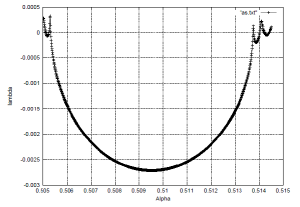
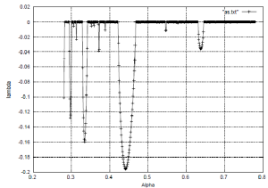
Figure 9: Left-hand figure: The Lyapunov exponent $\lambda$ in the region of the commensurate step $q=1/6$, for $\beta=0.36$ and $\gamma=0$ with $k=2$ corresponding to figure 6 given in [6]. Right-hand figure: Graph of the Lyapunov exponent $\lambda$: $\beta=0.23$ and $\gamma=0$ with $k=4$ corresponding to figure 4 in [6].

The logarithm of the biggest eigenvalue of the matrix plays the same role for a generic attractor as it does for a basic fixed point. It can also be seen numerically that $\lambda$ is never considerably positive [6] (see figures in 9). The figures in 9 were taken from the reference [6]. Non-zero Lyapunov exponent quantifies the exponential rate of growth or decay of the initial perturbation obtained as a time average with $t\rightarrow\infty$. The Lyapunov exponent vanishing indicates that the set of trajectories is quasi-continuous, or in other words, that it has a zero frequency “phason” mode [2] (for more information, see [5]).

The Lyapunov exponent also indicates whether an infinitesimal change in the beginning conditions will have an infinitesimal influence (negative exponent) or will result in a completely different trajectory (positive exponent) [2]. For the Ising model corresponding to the Hamiltonian (3.15), the paramagnetic region in phase diagrams disappeared, because the limit

$$\underset{n\to\infty}{\mathop{\lim}}\,({{x}^{(n)}},y_{1}^{(n)},y_{2}^{(n)})=({{x}^{*}},0,0)$$

is not satisfied.

3.5 The stability of the paramagnetic phase

To obtain the stability limit surface of the paramagnetic phase, we study the stability of paramagnetic phase. Thus, we need to linearize equations (3.22)–(3.24) around the fixed point $(x^{*},0,0)$, where $x^{*}$ is given by

$$x^{*}=f(x^{*},0,0)=\frac{{{({{b}^{2}}x^{*}+{{c}^{2}})}^{k}}+{{(1+{{b}^{2}}{{c}^{2}}x^{*})}^{k}}}{{{a}^{2}}{{({{b}^{2}}{{c}^{2}}+x^{*})}^{k}}+{{({{c}^{2}}x^{*}+{{b}^{2}})}^{k}}}.$$ (3.28)

In general, the behavior of solutions to a linear or linearized system can be predicted based on the eigenvalues of the Jacobian matrix. Negative eigenvalues cause a solution to tend towards zero, positive eigenvalues cause the solution to approach infinity, and imaginary eigenvalues cause a spiral behavior of solutions.

Theorem 3.2

(Liapunov’s Theorem). Let $f:\mathbf{R}^{n}\rightarrow\mathbf{R}^{n}$ be $C^{1}$ and $x_{0}\in\mathbf{R}^{n}$ be a fixed point of $x^{\prime}=f(x)$ (so $f(x_{0})=0)$. Let $A=Df(x_{0})$ be the linearization of $f$ (so $A_{ij}=\partial f_{i}/\partial x_{j}$ is the Jacobian matrix) and $\lambda_{1},\ldots,\lambda_{n}$ be its eigenvalues. Then, $x_{0}$ is

• asymptotically stable if $Re\lambda_{i}<0$ for all $i=1,\ldots,n$;

• unstable if $Re\lambda_{i}>0$ for some $i$.

Note that if the real parts of the eigenvalues are all zero, then further analysis is necessary. Let us consider the equations (3.23) and (3.24), we have

$$J = \left(\begin{matrix}\frac{\partial{{F}_{2}}({{x}_{n}},{{y}_{n}},{{z}_{n}})}{\partial{{y}_{n}}}&\frac{\partial{{F}_{2}}({{x}_{n}},{{y}_{n}},{{z}_{n}})}{\partial{{z}_{n}}}\\ \frac{\partial{{F}_{3}}({{x}_{n}},{{y}_{n}},{{z}_{n}})}{\partial{{y}_{n}}}&\frac{\partial{{F}_{3}}({{x}_{n}},{{y}_{n}},{{z}_{n}})}{\partial{{z}_{n}}}\\ \end{matrix}\right),$$ (3.29)

where

$$\frac{\partial F_{2}(x_{n},y_{n},z_{n})}{\partial y_{n}} = \frac{4b^{2}k\left(b^{2}c^{2}+x^{*}\right)^{k-1}\left(b^{2}+c^{2}x^{*}\right)^{k-1}\left(2b^{2}c^{2}+x^{*}+c^{4}x^{*}\right)}{\left(\left(b^{2}c^{2}+x^{*}\right)^{k}+\left(b^{2}+c^{2}x^{*}\right)^{k}\right)^{2}},$$

$$\frac{\partial F_{2}(x_{n},y_{n},z_{n})}{\partial z_{n}} = \frac{4k\left(b^{2}c^{2}+x^{*}\right)^{k-1}\left(b^{2}+c^{2}x^{*}\right)^{k-1}\left(b^{2}+b^{2}c^{4}+2c^{2}x^{*}\right)}{\left(\left(b^{2}c^{2}+x^{*}\right)^{k}+\left(b^{2}+c^{2}x^{*}\right)^{k}\right)^{2}},$$

$$\frac{\partial F_{3}(x_{n},y_{n},z_{n})}{\partial y_{n}} = \frac{4b^{2}k\left(b^{2}c^{2}+x^{*}\right)^{k-1}\left(b^{2}+c^{2}x^{*}\right)^{k-1}\left(2b^{2}c^{2}+x^{*}+c^{4}x^{*}\right)}{\left(\left(b^{2}c^{2}+x^{*}\right)^{k}+\left(b^{2}+c^{2}x^{*}\right)^{k}\right)^{2}},$$

$$\frac{\partial F_{3}(x_{n},y_{n},z_{n})}{\partial z_{n}} = \frac{4k\left(b^{2}c^{2}+x^{*}\right)^{k-1}\left(b^{2}+c^{2}x^{*}\right)^{k-1}\left(b^{2}+b^{2}c^{4}+2c^{2}x^{*}\right)}{\left(\left(b^{2}c^{2}+x^{*}\right)^{k}+\left(b^{2}+c^{2}x^{*}\right)^{k}\right)^{2}}.$$

It is clear that there exists at most two eigenvalues of the matrix (3.29). In this case, we have two different situations.
Let $\lambda_{1},\lambda_{2}$ be eigenvalues of the matrix (3.29).

• If $\lambda_{1},\lambda_{2}\in\mathbf{R}$, then the corresponding phase is either paramagnetic or ferromagnetic.

• If $\lambda_{1}=\overline{\lambda_{2}}\in\mathbf{C}$, then the fixed point is approached in an oscillatory way and the stability limit (which coincides with the critical limit for the second order phase transitions) is achieved if we consider the modulus of $\lambda$ equal to unity [3].

3.5.1 The Para-Ferro Transition

The variable $x_{n}$ is unaffected in the first order in $y_{n}$ and $z_{n}$, and in a matrix form, the linearized equations are given by

$$\left(\begin{array}[]{c}y_{n+1}\\ z_{n+1}\end{array}\right)=2L_{n}\left(\begin{array}[]{c}y_{n}\\ z_{n}\end{array}\right).$$ (3.30)

In this case, then the corresponding matrix is given by

$$L_{n}=\left(\begin{matrix}\frac{\partial{{F}_{2}}({{x}_{n}},{{y}_{n}},{{z}_{n}})}{\partial{{y}_{n}}}&\frac{\partial{{F}_{2}}({{x}_{n}},{{y}_{n}},{{z}_{n}})}{\partial{{z}_{n}}}\\ \frac{\partial{{F}_{3}}({{x}_{n}},{{y}_{n}},{{z}_{n}})}{\partial{{y}_{n}}}&\frac{\partial{{F}_{3}}({{x}_{n}},{{y}_{n}},{{z}_{n}})}{\partial{{z}_{n}}}\\ \end{matrix}\right)=\left(\begin{array}[]{cc}\frac{b^{2}}{b^{2}+x}&\frac{1}{b^{2}+x}\\ -\frac{x}{1+b^{2}x}&-\frac{xb^{2}}{1+b^{2}x}\end{array}\right).$$

For $c=1$, if the eigenvalues of the matrix $L_{n}$ in (3.30) are real, the situation occurs when this largest eigenvalue is equal to 1:

$$3x^{2}+\left(\frac{5}{b^{2}}-3b^{2}\right)x-1=0,$$

with $x$ positive. As a result, the equation for the para-ferro transition line is $a=f(b)$, with $a=\exp(J_{1}/T),b=\exp(J_{p}/T)$ (see [2] for details).

3.5.2 The Para-Modulated Transition

The fixed point is approached in an oscillatory manner if the eigenvalues of the matrix $L_{n}$ in (3.30) with $c=1$ are complex. This is the regular lattice’s analogue of a tree of a periodic perturbation, where $q$ is the modulation wave-vector [2].

3.6 Strange Attractor

Why do we investigate a strange attractor and what is the contribution? As examined in the section 3, by means of the recursion relations associated with a given Hamiltonian we can plot the (numerically) exact phase diagram of the model by fixing some given parameters $\alpha,\beta,\gamma$ in the $(\alpha,\beta,\gamma)$ space. Yokoi et al. [4] provided substantial numerical evidence for chaotic phases linked with strange attractors for the Ising model with competing interactions on a Cayley tree. One may undertake a more extensive classification of these modulated phases by considering the strange attractors of the general modulated phases. One also computes the Lyapunov exponents to detect the presence of chaotic structures corresponding to a strange attractor of the map [79].

In addition, each phase is defined by a specific attractor in the $(X_{r},K_{r})$ plane, and the phase diagram is created by tracking the evolution of these attractors and detecting qualitative changes. Ganikhodjaev and Nawi [81] investigated the stange attractors associated with the antiphase with period 4, the antiferromagnetic phase with period 2 and the paramagnetic phase for an Ising model. The fractal character of the attractor associated with the chaotic phase was confirmed by the calculation of the Hausdorff dimension (see [40]).

By summing over successive shells from the outermost ($r=1$) to innermost $(r=N)$ shell, Inawashiro et al. [29] obtained recurrence relations for effective fields $X_{r}$ and NN-interactions $K_{r}$ which are rigorous, but which must in general be analyzed numerically. In order to plot strange attractors with a given Ising model, we consider the approach given in ref. [29].

In this context, graphs of some relevant strange attractors associated to Ising model on Cayley tree of arbitrary order have been plotted [63]. In [4], the occurrence of chaotic phases associated with strange attractors is supported by extensive numerical evidence. Moreover, Yokoi et al. [4] performed calculations to show the existence of a complete devil’s staircase at low temperatures. In [63], in the presence of an external magnetic field, we investigated the Vannimenus model on an arbitrary order Cayley tree with competing for nearest-neighbor and next-nearest-neighbor interactions. We obtained robust recurrence relations for effective fields $X_{r}$ and nearest-neighbor interactions $K_{r}$, although they must be studied numerically in general. The role of the external magnetic field was clarified.

The phase diagram is obtained by watching the evolution of these attractors and detecting qualitative changes. These changes might be continuous or abrupt, indicating second- or first-order transitions, respectively [4]. Therefore, studying the strange attractors is very important to characterize the phase diagrams associated with the relevant models.

In [40], Tragtenberg and Yokoi developed some efficient numerical procedures for this purpose. They also investigated the existence of strange attractors on the model in the presence of a field. In [81], the phase diagram of the recursive equations corresponding to this model was investigated using an iterative scheme developed for a renormalized effective nearest-neighbor coupling $K_{r}$ and effective field per site $X_{r}$ for spins on the $n$-th level of a Cayley tree with competing one-level $J_{0}$ and prolonged $J_{p}$ next-nearest-neighbor interactions between Ising spins on the tree. Using the approach proposed by Inawashiro et al. [30], they were able to get an intermediate range of $J_{p}/J_{0}$ values where $X_{r}$ and $K_{r}$ iterate to a finite attractor in the $X-K$ plane.

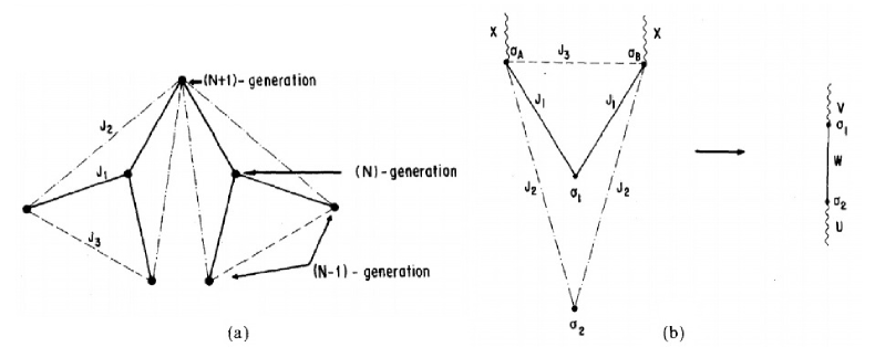
Figure 10: (a) Two successive generations of a Cayley tree (dot-dash line: prolonged second neighbor interactions; double dot-dash line: one-level second neighbor interactions). (b) Schematic diagram to illustrate the summation used in equation 2 (see [81]).

Let us consider the following Hamiltonian with spin values in $\Phi=\{-1,+1\}$, the relevant Hamiltonian with competing nearest-neighbor and prolonged next-nearest-neighbor binary interactions

$$H(\sigma)=-J_{1}\sum_{\langle x,y\rangle}\sigma(x)\sigma(y)-J_{2}\sum_{\rangle x,y\langle}\sigma(x)\sigma(y)-J_{3}\sum_{x\in V}\prod_{y\in S(x)}\sigma(y)-h\sum_{x\in V}\sigma(x),$$ (3.31)

where the sum in the first term ranges over all nearest neighbors, the second sum ranges over all prolonged next-nearest-neighbors, the third sum ranges over all one-level $k$-tuple neighbors and the spin variables $\sigma(x)$ assume the values $\pm 1$. Here, $J_{1},J_{2},J_{3},h\in\mathbf{R}$ are coupling constants (see figure 10).

In [63], we have obtained recursion relations for effective fields $X_{r}$ and nearest-neighbor interactions $K_{r}$, but they must be numerically investigated. The role of the external magnetic field has been clarified. We sum consecutively over spins to set up the iterative system, as shown schematically in figure 10 (see [63]). After performing basic but sophisticated algebraic operations, we obtained the following equations;

$$\exp[W\sigma_{1}\sigma_{2}+U\sigma_{1}+V\sigma_{2}]=$$

$$\frac{1}{C}\sum_{\sigma_{A_{i}}=\pm 1}\exp\left[(K_{1}\sigma_{1}+K_{2}\sigma_{2})\sum_{i=1}^{k}\sigma_{A_{i}}+K_{3}\sum_{i=1<j}^{k}\sigma_{A_{i}}\sigma_{A_{j}}+X\sum_{i=1}^{k}\sigma_{A_{i}}\right],$$ (3.32)

where $K_{i}\equiv J_{i}/(k_{\text{B}}T),i=1,2,3$ and we get

$$\left\{\begin{array}[]{l}U(X,K_{1},K_{2},K_{3})\equiv U=\frac{1}{4}\ln\frac{\omega(1,1)\omega(1,-1)}{\omega(-1,1)\omega(-1,-1)},\\ V(X,K_{1},K_{2},K_{3})\equiv V=\frac{1}{4}\ln\frac{\omega(1,1)\omega(-1,1)}{\omega(1,-1)\omega(-1,-1)},\\ W(X,K_{1},K_{2},K_{3})\equiv W=\frac{1}{4}\ln\frac{\omega(1,1)\omega(-1,-1)}{\omega(1,-1)\omega(-1,1)},\\ C(X,K_{1},K_{2},K_{3})\equiv C=\sqrt[4]{\omega(1,1)\omega(-1,-1)\omega(1,-1)\omega(-1,1)},\end{array}\right.$$ (3.37)

where the value of $\omega$ changes according to the oddness or evenness of the order $k$ of the tree. Therefore, we take $k$ as an odd number, and we obtain

$$\omega(\sigma_{1},\sigma_{2})=2\sum_{i=1}^{\frac{k-1}{2}}C(k,i)\exp\left[\frac{k^{2}-4ki-k+i^{2}+3i}{2}K_{3}\right]\cosh\left[(k-2i)(K_{1}\sigma_{1}+K_{2}\sigma_{2}+X)\right],$$

and if we take $k$ as an even number, we get the following equation,

$$\omega(\sigma_{1},\sigma_{2}) = 2\sum_{i=1}^{\frac{k}{2}-1}C(k,i)\exp\left[\frac{k^{2}-4ki-k+i^{2}+5i}{2}K_{3}\right]\cosh\left[(k-2i)(K_{1}\sigma_{1}+K_{2}\sigma_{2}+X)\right]$$

$$+ C(k,k/2)\exp\left[\frac{3k(2-k)}{8}K_{3}\right].$$

Starting with $X^{(1)}=B=h/(k_{\text{B}}T)$ and $K^{(1)}_{1}=K_{1}=J_{1}/(k_{\text{B}}T)$, where $h$ is the initial applied magnetic field per site and $J_{1}$ is the initial nearest-neighbor coupling, we obtain from the above equalities the iteration scheme, for $r=2,3,\ldots,N,$

$$X^{(r)} = B+kU(X^{(r-2)},K^{(r-2)}_{1},K_{2},K_{3})+V(X^{(r-1)},K^{(r-1)}_{1},K_{2},K_{3}),$$ (3.38)

$$K^{(r)}_{1} = K_{1}+W\left(X^{(r-1)},K^{(r-1)}_{1},K_{2},K_{3}\right).$$ (3.39)

Using the $U,V$ and $W$ functions given in (3.37), we have obtained recursive relations (3.38) and (3.39). Taking into account the initial conditions $X^{(0)}=K^{(0)}_{1}=0$ and $X^{(1)}=B,K^{(0)}_{1}=K_{1}$, the graphs of the strange attractor are plotted.

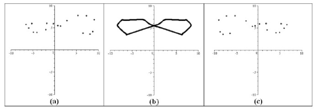
Figure 11: The attractors in $X-K_{1}$ plane for $k=2$, $\gamma=\frac{J_{3}}{J_{1}}=-0.38$, $\beta=\frac{J_{2}}{J_{1}}=0.38$, and $\alpha=\frac{k_{b}T}{J_{1}}=0.11$ with external magnetic for (a) $\delta=\frac{h}{J_{1}}=+0.1$, (b) $\delta=\frac{h}{J_{1}}=0$ and (c) $\delta=\frac{h}{J_{1}}=-0.1.$

We have obtained some attractor graphs in figures 11 [63]. The corresponding phase is incommensurate for $h=0$, but it turns into a commensurate phase with the presence of an external magnetic field. Attractors in both figure 11 (a) and figure 11 (c) reflect the commensurate phase. We refer the readers to [63] for detailed information.

3.7 Notes and remarks

For the Cayley tree of finite order, the system of nonlinear equations have been successfully derived in [6, 46]. When the prolonged next nearest coupling constant is added to the Hamiltonian examined by Vannimenus instead of the next nearest coupling constant [38, 46], a considerable change is observed in the phase diagrams. In this case, the paramagnetic (P) phase region is completely lost in the phase diagrams corresponding to the model in [46] on the $[-2,2]\times[-2,2]$. As $k$ increases, it is seen that some phase regions have narrowed or even disappeared (see [46] for details).

During the studies obtained for both Ising models and Potts models, very different phase types were encountered in the form of narrow islands in the phase diagrams. We cannot determine why these islands actually exist. These islands may have originated from the drawing. For this reason, in order to determine the species of these islands, Lyapunov exponents and drawing of the wave vectors were needed (see figure 7).

In contrast to [2] and Mariz [3], the stability analysis for the ferromagnetic phase is more difficult than the stability analysis for the paramagnetic phase because the fixed point is not the same for the whole phase. Therefore, in order to study the stability analysis of the ferromagnetic phase for the model (3.15), we need new methods.

In [29], Inawashiro et al have considered schematic illustration of selective summation of spins from the outermost to innermost shells to plot the phase diagrams of the Ising model. They set up an iterative scheme for Vannimenus’s equations [2]. They obtained a phase diagram containing ferromagnetic (F), paramagnetie (P), chaotic (C), and antiferromagnetic + + – – (A) phases. Silva et al. [9] consider a very general model on Bethe lattices of arbitrary branching number with arbitrary couplings between: $(J_{1})$ first-, $(J_{2})$ second- and $(J_{3})$ third-neighbors, and furthermore in the presence of an arbitrary external field. In particular, in [9], for $J_{3}=0$, the model reduces to the model analyzed in [61], i.e., the generalization of the Vannimenus model to arbitrary order number.

When we investigated the phase diagrams given in our recent articles, very rich and different new phases were obtained. The structure of the phase diagrams of the generalized systems was examined and compared [6, 46, 61]. Magnetization graphs were plotted for certain gamma and beta values. Lyapunov exponents were successfully plotted for certain values of $k$ and for certain critical coupling constants [6]. The stability analysis of the given system was examined in detail.

In addition, the transition lines between the phases were successfully investigated. This work was published in [16]. Finally, for Ising model on a Cayley tree of arbitrary order, a system of nonlinear equations corresponding to the Hamiltonian of 3 different interactions was obtained and the phase analysis was successfully performed and this work was published in [82]. Since more comprehensive information and findings are included in the related studies, details are not given here (see [6, 46, 61] for details).

In [83], the phase diagrams of an Ising model involving nearest neighbor $J$, triplet prolonged next nearest neighbor $J_{p}$ and one-level next nearest neighbor $J_{1_{l}}$ on the third order Cayley tree were plotted. Despite the presence of paramagnetic regions in the phase diagrams obtained in previous studies [2, 3, 84], the paramagnetic phase zones for the low temperatures in the work [83] completely disappeared.

We see that ternary prolonged next nearest interaction has strong effects on the phase diagrams. One of these is the shift from the zero temperature values of the multi-critical Lifshits points to the end values. The other effect is the disappearance of paramagnetic phase zones. For some given coupling constants $J$, $J_{p}$ and $J_{1_{l}}$, the plots of the wave vectors are interpreted.

4 The dynamical behavior of Potts model on a Cayley tree

In this section, we study the phase diagrams of a $q$-state Potts models having certain characteristics. Notably, we should mention that most of the results were published in previous studies. Our goal here is to interpret the results by comparing them.

It is well-known that the $q$-state Potts models are generalizations of the 2-state Ising model, which is equivalent to $q=2$ in this case. The Potts model can be expressed as a class of the statistical mechanics models that specifically examine the long-term behavior of complex systems [32]. These models have a rich structure in order to sample almost every subject area. In particular, it is at the center of investigations by the intersection of conformal field theory, infiltration theory, quantum groups and integrable systems. The Potts model explores the interactions of system elements based on certain characteristics of each element [47]. The Potts model has a powerful mathematical modelling method that can be used in a variety of disciplines, including biology, sociology, physics, and chemistry [55, 73, 85, 86].

For all values of the external magnetic field and temperature, Peruggi et al. [87] studied the $q$-state ferromagnetic Potts model (FPM) and antiferromagnetic Potts model (APM). They derived exact formulas for all thermodynamic functions of relevance in the FPM and APM, as well as drew entire phase diagrams for both systems. By using the method of solution of spin models on Cayley tree, Peruggi et al. [88] analyzed the phases of the ferromagnetic and antiferromagnetic $q$-state Potts models. Nevertheless, in the literature, the phase diagrams for the Potts models, except a few publications, have not been solved and compared using any computer programs ([17, 41, 60, 89, 90, 91]). For this reason, it has taken some time for the codes to be created. In general, deriving the recurrence equations associated to the Potts models is much more difficult than in the Ising model. Especially, as the number of the branches of the Cayley tree increases, it becomes even more difficult to derive the recurrence equations [92, 93].

In this section, we are going to explain how the phase diagrams are analyzed, taking into account some Potts models that we studied before.

4.1 The $q$-state Potts model with three different binary competing interactions on a Cayley tree

Let us consider the Hamiltonian given by

$$H(\sigma)=-J_{1}\sum_{\langle x,y\rangle}\delta_{\sigma(x)\sigma(y)}-J_{p}\sum_{\rangle x,y\langle}\delta_{\sigma(x)\sigma(y)}-J_{o}\sum_{\rangle\widetilde{x,y}\langle}\delta_{\sigma(x)\sigma(y)},$$ (4.1)

where the coupling constants are referred to as competing nearest-neighbor (NN) interaction $J_{1}$, prolonged next-nearest-neighbor (PNNN) interaction $J_{p}$ and one-level next-nearest-neighbor (1LNNN) interaction $J_{o}$, respectively (see [41] for details). In order to study the behavior of the recursive relations associated to the Hamiltonian given in (4.1), we established an iterative scheme similar to that appearing in real space renormalization group frameworks (RSRGF) [76]. In this system, the nearest neighbor interactions with the triplets on the Cayley tree of the order two were considered and we observed the presence of the ferromagnetic and the paramagnetic phase regions in the phase diagrams, as well as in a new phase region called the paramodulated phase (see figure 12). Corresponding phase diagrams were plotted by means of the coupling constants $J_{1},J_{p}$ and $J_{o}$. At finite temperatures, we determined several interesting features exhibited for some typical values of $J_{o}/J_{1}$.

After tedious calculations, we obtained the sequence

$$[x^{(n+1)},y_{1}^{(n+1)},y_{2}^{(n+1)},y_{3}^{(n+1)}].$$ (4.2)

The system of four equations obtained in (4.2) has a more complex structure than the recurrence equations of the Vannimenus-Ising model and Potts model associated with the Hamiltonian (4.3).

By means of the recursive relations given in (4.2), we were interested in the exact phase diagrams in three-dimensional space $(T/J_{1},-J_{p}/J_{1},J_{o}/J_{1})$. Here, instead of drawing in 3 dimensions, we plotted phase diagrams in two dimensions without considering one of these expressions. We iterate the recursive equations (4.2) and analyze their behavior after a large number of iterations by starting with initial conditions $(x^{(1)},\,\,y_{1}^{(1)},\,\,y_{2}^{(1)},\,\,y_{3}^{(1)})$ corresponding to boundary condition $\overline{\sigma}^{(n)}(V\setminus V_{n})\equiv 1$.

In order to plot the phase diagrams associated to a given model, we try to find a fixed point $(x^{(*)},y_{1}^{(*)},\,\,y_{2}^{(*)},y_{3}^{(*)})$. If $y_{1}^{(*)}=0,\,\,y_{2}^{(*)}=0,\,\,y_{3}^{(*)}=0$, it corresponds to a paramagnetic phase (white colour) or if $y_{1}^{(*)}\neq 0,\,\,y_{2}^{(*)}\neq 0,\,\,y_{3}^{(*)})\neq 0$, then it corresponds to a ferromagnetic phase ’FERROMAGNETIC’. Secondly, the recursive system of equations may have an iterative state with period $p$ (see the table 1). If we obtain as $p=2$, the phase corresponds to antiferromagnetic phase (or ’PERIOD 2’) and in the case $p=4$, the type of phase corresponds to the so-called antiphase (’PERIOD 4’), that is denoted $\left\langle 2\right\rangle$ for brevity. If $p=5,6,7,8,9,10,11$, then the relevant phases are called ’PERIOD 5’, ’PERIOD 6’, ’PERIOD 7’, ’PERIOD 8’, ’PERIOD 9’, ’PERIOD 10’ and ’PERIOD 11’, respectively (see [41] for details).

Finally, the system can continue to be aperiodic, that is, in case of not reaching a certain fixed period. It is difficult to quantitatively determine the difference between a really aperiodic example and the one with a very long period. Having a period of $p$ ($p\leqslant 12$) is considered to be a periodic phase. We shall recall all periodic phases with a period of $p>12$ and aperiodic phase as the modulated phases ’MODULATED’ (see the table 1 for details).

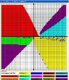
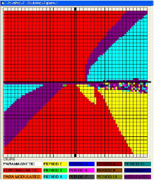
Figure 12: (Colour online) Left-hand: The phase diagram of the recursive relations corresponding to the Hamiltoninan (4.1) for $\gamma=0$ on the rectangular region $[-2,2]\times[-2,2]$. Right-hand: Phase diagram of the recursive relations for $\gamma=1$ on the rectangular region $[-2,2]\times[-2,2]$ (see [41])

Figures given in 12 show the phase diagrams corresponding to the Potts model presented in [41]. The phase regions according to the third parameter variable values $\gamma$ are seen in figures given in 12. We observed that for given values of these phase zones, our diagrams contained the paramagnetic region and we obtained the multi-critical Lifshitz points for the increasing values of temperature.

4.2 The Potts model with two interactions on a Cayley tree

Let us consider the following Hamiltonian as the counterpart of the Ising model for the Hamiltonian given by Ganikhodjaev et al. [38]

$$H(\sigma)=-{{J}_{p}}\sum\limits_{\langle\widetilde{x,y,z}\rangle}{{{\delta}_{\sigma(x)\sigma(y)\sigma(z)}}}-J\sum\limits_{\langle x,y\rangle}{{{\delta}_{\sigma(x)\sigma(y)}}}.$$ (4.3)

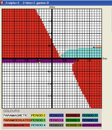
Figure 13: (Colour online) Phase diagram of the recursive relations associated to the Potts model with triple and binary interacting on the rectangular region $[-2,2]\times[-2,2]$ (see [89]).

The dynamical system for the Potts model associated with the Hamiltonian (4.3) on the Cayley tree of the order 2 is studied in [89]. We analyzed the phase diagram of the Potts model with competing prolonged ternary and binary NN interactions and demonstrated that it consisted of the following phases: ferromagnetic, paramagnetic, and antiphase with period 4, and modulated phase (figure 13) [89]. Unlike the Vannimenus-Ising model given in (3.1), the paramagnetic phase for this model (4.3) was observed in a large region (see figure 13).

The set of spin values $\{1,2,3\}$ associated with the Hamiltonian (4.3) can be replaced by the centered set $\{-1,0,1\}$ since the form of spins of the Potts model associated with the Hamiltonian (4.3) is unessential. Therefore, the average magnetization $\tilde{m}$ for the $n\,$th generation is calculated as follows:

$$\tilde{m}=-\frac{4(y_{1}+y_{2})(2x+y_{2}+1)}{(2x+y_{1}+2y_{2}+1)^{2}+2(2x-y_{1}+1)^{2}}.$$

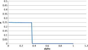
Figure 14: (Colour online) Variation of the wave-vector $q$ versus $T$, for $\beta=-J_{p}/J_{1}=0.8$ (see [89]).

Figure 14 shows how the wave-vector changes as a function of temperature $T$ between its value at the paramodulated transition and its value in the $\left\langle 2\right\rangle$ phase is equal to $\frac{1}{4}$ (the figure 14 is borrowed from [89]).

If we take into account the Ising model introduced in [38], we could not get the fixed point $(x^{*},0,0)$, but we obtained the fixed points when we considered the Potts model with the same Hamiltonian. Furthermore, we observed the presence of the paramagnetic phase regions in the phase diagram of the Potts model (see figure 13).

Remark 4.1

Note that the same Potts model on a Cayley tree of arbitrary order can be numerically studied. However, deriving the recursive equations for the same Potts model is a difficult problem. Exact description of the phase diagrams and recurrence equations is rather tricky.

4.3 The 3-state Potts model on Cayley tree of the order 2

This subsection is based on the paper [17]. Consider the three-state Potts model with spin values $\Phi=\{1,2,3\}$. The relevant Hamiltonian takes the form with competing binary nearest-neighbor and two separate ternary interactions as follows [17]:

$$H(\sigma)=-{{J}_{p}}\sum\limits_{\langle\widetilde{x,y,z}\rangle}{{{\delta}_{\sigma(x)\sigma(y)\sigma(z)}}}-{{J}_{t}}\sum\limits_{\langle x,\widetilde{y},z\rangle}{{{\delta}_{\sigma(x)\sigma(y)\sigma(z)}}}-{{J}_{1}}\sum\limits_{\langle x,y\rangle}{{{\delta}_{\sigma(x)\sigma(y)}}},$$ (4.4)

where $J_{p},J_{t},J_{1}\in\mathbf{R}$ are coupling constants and $\delta$ is the Kronecker symbol and defined as

$${{\delta}_{\sigma(x)\sigma(y)\sigma(z)}}=\left\{\begin{matrix}1,\text{ if }\sigma(x)=\sigma(y)=\sigma(z)\text{ }\\ 0,\text{ otherwise}\text{. \ \ \ \ \ \ \ \ \ \ \ \ \ \ \ }\\ \end{matrix}\right.$$

The system of nonlinear equations associated with the Hamiltonian given by equation (4.4) is numerically analyzed in [17]. By analyzing the recurrence equations numerically, we showed that the phase diagrams contained ferromagnetic, paramagnetic and $\left<2\right>$ phases only. We also saw that the modulated phases contained only the $\left<2\right>$ for $J_{1}>0$ and $J_{p}/J_{1}<0$. We obtained the transition lines by means of stability conditions. We looked at the characteristic properties of the phase diagram using numerical iterations. For some critical points in the modulated phases, we plotted the wave-vectors versus temperature.

4.3.1 Recurrence equations

Here, we give the recursion equations for the sake of completeness (see [17] for details). We investigate the relationship between the partition function on $V_{n}$ and the partition function on subsets of $V_{n-1}$ to generate the recurrent equations. The recurrence equations show how their impact propagates along the tree having got the initial conditions on $V_{1}$. We will look at the partition functions herein below.

Let $Z_{i}^{(n)}$ be a partition function on $V_{n}$ such that the spin $i$ in the root (node) $x^{(0)}$, $i=1,2,3;$ let $Z^{(n)}(i,j)$ be a partition function on $V_{n}$ with the configuration $(i,j)$ on an edge $\langle x^{(0)},x\rangle$. To continue this process, we consider all interactions except interaction of nearest neighbors $\langle x^{(0)},x\rangle,\,x\in W_{1}$ and $i,j=1,2,3;$ let $Z^{(n)}(i_{1},i_{0},i_{2})$ be a partition function on $V_{n}$, where spin $i_{0}$ is placed at vertex $x^{(0)}$ and spins $i_{1}$ and $i_{2}$ are placed at the next vertices $x_{1}$ and $x_{2}$ belonging to $S(x^{(0)})$.
If the set of spins is taken as $\Phi=\{1,2,3\}$, the number of partition functions $Z^{(n)}\left(\begin{array}[]{ccc}i_{1}&&i_{2}\\ &i_{0}&\end{array}\right)=Z^{(n)}(i_{1},i_{0},i_{2})$ is 27 (see figure 15) and the total partition function $Z^{(n)}$ in the volume $V_{n}$ can be written as

$$Z^{(n)}=\sum^{3}_{i_{1},i_{0},i_{2}=1}Z^{(n)}(i_{1},i_{0},i_{2})=\sum^{3}_{i_{1},i_{0},i_{2}=1}Z^{(n)}\left(\begin{array}[]{ccc}i_{1}&&i_{2}\\ &i_{0}&\end{array}\right).$$ (4.5)

Figure 15: (Colour online) A configuration on $V_{1}$.

$$Z^{(n)}(i_{1},i_{0},i_{2}) = \exp\left(\frac{J_{t}}{2T}\delta_{i_{1}i_{0}i_{2}}+\frac{J_{1}}{T}\delta_{i_{0}i_{1}}+\frac{J_{1}}{T}\cdot\delta_{i_{0}i_{2}}\right)Z^{(n)}\left(\begin{array}[]{cc}i_{1}&\\ &i_{0}\end{array}\right)Z^{(n)}\left(\begin{array}[]{cc}&i_{2}\\ i_{0}&\end{array}\right)$$ (4.10)

$$= \exp\left(\frac{J_{t}}{2T}\delta_{i_{1}i_{0}i_{2}}+\frac{J_{1}}{T}\delta_{i_{0}i_{1}}+\frac{J_{1}}{T}\delta_{i_{0}i_{2}}\right)Z^{(n)}(i_{0},i_{1})Z^{(n)}(i_{0},i_{2}),$$ (4.11)

where $i_{1},i_{0},i_{2}\in\{1,2,3\}.$

If we take into account all partition functions in the volume $V_{n}$ under the boundary condition $\bar{\sigma}_{n}\equiv 1,$ then we assume

$$Z^{(n)}(1,2) = Z^{(n)}(1,3),\ Z^{(n)}(2,1)=Z^{(n)}(3,1),$$ (4.12)

$$Z^{(n)}(2,2) = Z^{(n)}(3,3),\ Z^{(n)}(2,3)=Z^{(n)}(3,2).$$ (4.13)

For the sake of completeness, we again recall the equations that we obtained herein below earlier.

Let $a=\exp\left(\frac{J_{t}}{2T}\right)$; $b=\exp\left(\frac{J_{p}}{T}\right)$, $c=\exp\left(\frac{J_{1}}{T}\right)$. From (4.10), we have the partial partition equations as follows.
First, for $\sigma(x^{(0)})=1$ we obtain

$$Z^{(n)}(1,1,1) = a^{2}c^{2}(Z^{(n)}(1,1))^{2},$$

$$Z^{(n)}(1,1,2) = Z^{(n)}(2,1,1)=cZ^{(n)}(1,1)Z^{(n)}(1,2),$$

$$Z^{(n)}(1,1,3) = Z^{(n)}(3,1,1)=cZ^{(n)}(1,1)Z^{(n)}(1,3),$$

$$Z^{(n)}(2,1,2) = Z^{(n)}(3,1,3)=(Z^{(n)}(1,2))^{2},$$

$$Z^{(n)}(2,1,3) = Z^{(n)}(3,1,2)=(Z^{(n)}(1,2))^{2}.$$

Secondly, for $\sigma(x^{(0)})=2$ we get

$$Z^{(n)}(1,2,1) = (Z^{(n)}(2,1))^{2},$$

$$Z^{(n)}(1,2,2) = Z^{(n)}(2,2,1)=cZ^{(n)}(2,1)Z^{(n)}(2,2),$$

$$Z^{(n)}(1,2,3) = Z^{(n)}(3,2,1)=Z^{(n)}(2,1)Z^{(n)}(2,3),$$

$$Z^{(n)}(2,2,2) = a^{2}c^{2}(Z^{(n)}(2,2))^{2},$$

$$Z^{(n)}(2,2,3) = Z^{(n)}(3,2,2)=cZ^{(n)}(2,2)Z^{(n)}(2,3),$$

$$Z^{(n)}(3,2,3) = (Z^{(n)}(2,3))^{2}.$$

Thirdly, for $\sigma(x^{(0)})=3$ one gets

$$Z^{(n)}(1,3,1) = (Z^{(n)}(3,1))^{2},$$

$$Z^{(n)}(1,3,2) = Z^{(n)}(2,3,1)=Z^{(n)}(3,1)Z^{(n)}(3,2),$$

$$Z^{(n)}(1,3,3) = Z^{(n)}(3,3,1)=cZ^{(n)}(3,1)Z^{(n)}(3,3),$$

$$Z^{(n)}(2,3,2) = (Z^{(n)}(3,2))^{2},$$

$$Z^{(n)}(2,3,3) = Z^{(n)}(3,3,2)=cZ^{(n)}(3,2)Z^{(n)}(3,3),$$

$$Z^{(n)}(3,3,3) = a^{2}c^{2}(Z^{(n)}(3,3))^{2}.$$

Due to (4.12) and (4.13), we can select only five independent partition functions $Z^{(n)}(1,1,1)$, $Z^{(n)}(2,1,2)$, $Z^{(n)}(1,2,1)$, $Z^{(n)}(2,2,2)$, $Z^{(n)}(3,2,3)$ and therefore we can introduce new variables

$$\left\{\begin{array}[]{l}u_{1}^{(n)}=\sqrt{Z^{(n)}(1,1,1)},\\ u_{2}^{(n)}=\sqrt{Z^{(n)}(2,1,2)},\\ u_{3}^{(n)}=\sqrt{Z^{(n)}(1,2,1)},\\ u_{4}^{(n)}=\sqrt{Z^{(n)}(2,2,2)},\\ u_{5}^{(n)}=\sqrt{Z^{(n)}(3,2,3)}.\end{array}\right.$$

After tedious calculations, we have the following equations

$$\left\{\begin{array}[]{l}u_{1}^{(n+1)}=ac[b^{2}(u_{1}^{(n)})^{2}+4a^{-1}bu_{1}^{(n)}u_{2}^{(n)}+4(u_{2}^{(n)})^{2}],\\ u_{2}^{(n+1)}=[(u_{3}^{(n)})^{2}+2a^{-1}u_{3}^{(n)}u_{4}^{(n)}+2u_{3}^{(n)}u_{5}^{(n)}+(u_{4}^{(n)})^{2}+2a^{-1}u_{4}^{(n)}u_{5}^{(n)}+(u_{5}^{(n)})^{2}],\\ u_{3}^{(n+1)}=[(u_{1}^{(n)})^{2}+4a^{-1}u_{1}^{(n)}u_{2}^{(n)}+4(u_{2}^{(n)})^{2}],\\ u_{4}^{(n+1)}=ac[(u_{3}^{(n)})^{2}+2a^{-1}bu_{3}^{(n)}u_{4}^{(n)}+2u_{3}^{(n)}u_{5}^{(n)}+b^{2}(u_{4}^{(n)}){}^{2}+2a^{-1}bu_{4}^{(n)}u_{5}^{(n)}+(u_{5}^{(n)})^{2}],\\ u_{5}^{(n+1)}=[(u_{3}^{(n)})^{2}+2a^{-1}u_{3}^{(n)}u_{4}^{(n)}+2u_{3}^{(n)}u_{5}^{(n)}+(u_{4}^{(n)})^{2}+2a^{-1}u_{4}^{(n)}u_{5}^{(n)}+(u_{5}^{(n)})^{2}].\end{array}\right.$$ (4.14)

Since $u_{2}^{(n+1)}=u_{5}^{(n+1)}$, we can rewrite the system of equations given in (4.14) as

$$\left\{\begin{array}[]{l}u_{1}^{(n+1)}=ac[b^{2}(u^{(n)}_{1})^{2}+4a^{-1}bu^{(n)}_{1}u^{(n)}_{2}+4(u^{(n)}_{2})^{2}],\\ u_{2}^{(n+1)}=[(u^{(n)}_{2}+{u^{(n)}_{3}})^{2}+2a^{-1}(u^{(n)}_{2}+u^{(n)}_{3})u^{(n)}_{4}+{u^{(n)}_{4}}^{2}],\\ u_{3}^{(n+1)}=[(u^{(n)}_{1})^{2}+4a^{-1}u^{(n)}_{1}u^{(n)}_{2}+4(u^{(n)}_{2})^{2}],\\ u_{4}^{(n+1)}=ac[({u^{(n)}_{2}}+{u^{(n)}_{3}})^{2}+2a^{-1}b(u^{(n)}_{2}+u^{(n)}_{3})u^{(n)}_{4}+b^{2}(u^{(n)}_{4})^{2}].\end{array}\right.$$ (4.15)

In order to draw the phase diagram, we prefer the following choice;

$$x=\dfrac{u_{2}+u_{3}}{u_{1}+u_{4}},\quad y_{1}=\dfrac{u_{1}-u_{4}}{u_{1}+u_{4}},\quad y_{2}=\dfrac{u_{2}-u_{3}}{u_{1}+u_{4}}.$$

If we substitute as follows;

$$u_{1}=\frac{(1+y_{1})A}{2},\quad u_{2}=\frac{(x+y_{2})A}{2},\quad u_{3}=\frac{(x-y_{2})A}{2},\quad u_{4}=\frac{(1-y_{1})A}{2},$$

where $A=u_{1}+u_{4}$. Then, equations (4.15) yield:

$$\begin{array}[]{lll}x^{\prime}&=&\dfrac{1}{acD}[4x^{2}+4xy_{2}+2y_{2}^{2}+2a^{-1}(2x+y_{2}+y_{1}y_{2})+y_{1}^{2}+1];\\[8.53581pt] y^{\prime}_{1}&=&\dfrac{2}{D}[b^{2}y_{1}+a^{-1}b(2xy_{1}+y_{2}+y_{1}y_{2})+2xy_{2}+y_{2}^{2}];\\[8.53581pt] y^{\prime}_{2}&=&-\dfrac{2}{acD}[y_{1}+2xy_{2}+y_{2}^{2}+a^{-1}(2xy_{1}+y_{2}+y_{1}y_{2})],\end{array}$$ (4.16)

where $D=b^{2}(1+y_{1}^{2})+2a^{-1}b(2x+y_{2}+y_{1}y_{2})+4x^{2}+4xy_{2}+2y_{2}^{2}.$

In order to plot the phase diagram we have to look at the local properties, namely the local magnetization or the magnetization of the root $x^{(0)}.$ Since the spin form of the Potts model is unessential, the set of spin values $\{1,2,3\}$ can be replaced by the centered set $\{-1,0,1\}$. The average magnetization $\tilde{m}$ for the $n$ generation is then calculated as:

$$\tilde{m}=-\frac{(2x+y_{2})(a^{-1}y_{1}+y_{2})+y_{1}+a^{-1}y_{2}}{12x^{2}+3y_{1}^{2}+4y_{2}^{2}+8xy_{2}-2y_{1}+4a^{-1}(3x+y_{2}+y1y_{2}-xy_{1})}.\\$$ (4.17)

Thus, a situation where $y_{1}^{*}$, $y_{2}^{*}\neq 0$ but $\tilde{m}=0$ can occur. Considering the system of nonlinear equation (4.16) and the average magnetization equation (4.17) together, we draw the phase diagrams of the given Potts model using numerical calculations (see [17] for details).

4.3.2 The phase diagrams of the 3-state Potts model associated with the Hamiltonian (4.4)

Before delving deeper into the various transitions, it is helpful to understand the main aspects of the phase diagram. As we mentioned in detail in previous sections, the numerically precise phase diagrams are plotted by the recursive relations (4.16) in 3-dimensional space $(T/J_{1},-J_{p}/J_{1},J_{t}/J_{1})$. Based on the previous work, we make the following variable replacement; $(-J_{p}/J_{1})=\beta$, $T/J_{1}=\alpha$ and $J_{t}/J_{1}=\gamma$ and respectively $b=\exp(-\alpha^{-1}\beta)$, $c=\exp(\alpha^{-1})$ and $a=\exp((2\alpha)^{-1}\gamma).$ Then, we have $a=c^{\frac{\gamma}{2}}.$ For some given values of $\gamma$, under boundary condition $\bar{\sigma}^{(n)}\equiv 1,$ we obtain the initial conditions of the system of equations (4.16) as follows,

$$x^{(1)}=\dfrac{1+a^{2}c^{2}}{ac(a^{2}c^{2}b^{2}+1)},\quad y_{1}^{(1)}=\dfrac{a^{2}c^{2}b^{2}-1}{a^{2}c^{2}b^{2}+1},\quad y_{2}^{(1)}=\dfrac{1-a^{2}c^{2}}{ac(a^{2}c^{2}b^{2}+1)}.$$

The initial boundary conditions are iterated in the system of equations (4.16). By doing a sufficiently large number of iterations, we observe the behavior of the system of iterative equations (4.16) in the plane $(\beta=-\frac{J_{p}}{J_{1}},\alpha=\frac{T}{J_{1}}).$ As stated in the previous sections, it is aimed at reaching the fixed point $(x^{*},y_{1}^{*},y_{2}^{*})$, and phase diagrams are obtained according to the status of these fixed points (see table 1).

In order to investigate the limit behavior of Potts models associated to the Hamiltonian with different coupling constants on a Cayley tree of 2nd order, we have studied the systems of nonlinear equations corresponding to dynamical systems in order to realize the analysis of the dynamical systems of Hamiltonian equations for different interactions according to 3-valued ($q=3$) Potts model [17]. We should immediately say that to obtain recursive equations is becoming more difficult and time-consuming.

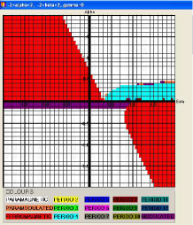
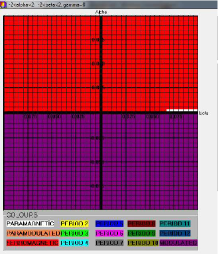
Figure 16: (Colour online) Left-hand: Phase diagram of the Potts model [17] for $\gamma=0$ on the rectangular region $[-2,2]\times[-2,2]$. Right-hand: The phase diagram of Potts model [17] for $\gamma=0$ on the rectangular region $[-0.1,0.1]\times[-0.1,0.1]$ (see [17] for the figure) (see [17] for the figure).

By examining the variation of the wave vectors, it is possible to determine the commensurate phases in the modulated regions. Looking at the related work, the regions in the considered phase diagrams are examined in smaller intervals and the transitions from one phase to the other are seen more clearly.

Let us use the fixed value $\gamma=0$ to see the diagrams. A two phase diagram is shown in figure 16. The modulated phase is reached in a very narrow interval $-0.11<\alpha<0$ with $\beta<0$ [see figure 16 (left)]. In order to investigate the phases with a very small mesh width of 0.005, in a more narrow square $[-0.1,0.1]\times[-0.1,0.1]$, the phase diagrams of the Potts model associated with the Hamiltonian (4.4) are plotted [see figure 16 (right)].

Remark 4.2

In the results that we have obtained as a team in the last decade, we followed the above method to investigate the dynamical behaviour of $q$-state Potts models and to plot the phase diagrams in detail (see [41, 17]).

4.4 The phase diagrams of 3-state Potts model on the Cayley tree of the order 3

As emphasized earlier, getting the recurrence equations associated to the Potts model is much more difficult compared to the Ising model. When the number of branches increases, it becomes even more difficult to find the recursive equations. The systems of nonlinear equations have been obtained for some Potts models with the competing interaction on the Cayley tree of arbitrary order. The behavior of the nonlinear dynamical systems corresponding to the Potts models obtained for Hamiltonians with various coupling constants on the Cayley tree has been studied.

Note that this subsection is based on the paper [60]. The appropriate Hamiltonian for the 3-state Potts model has the form with competitive NN, PNNN, and two-level triple interactions as:

$$H(\sigma)=-{{J}_{tt}}\sum\limits_{\langle\overline{x,y,z}\rangle}{{{\delta}_{\sigma(x)\sigma(y)\sigma(y)}}}-{{J}_{pn}}\sum\limits_{\rangle\widetilde{x,y}\langle}{{{\delta}_{\sigma(x)\sigma(y)}}}-{{J}_{nn}}\sum\limits_{\langle x,y\rangle}{{{\delta}_{\sigma(x)\sigma(y)}}},$$ (4.18)

where ${{J}_{tt}},{{J}_{pn}},{{J}_{nn}}\in\mathbb{R}$ are coupling constants and $\delta$ is the Kronecker symbol. Here, the function

$${{\delta}_{\sigma(x)\sigma(y)\sigma(y)}}=\left\{\begin{matrix}1;&\sigma(x)=\sigma(y)=\sigma(y)\\ 0;&\text{otherwise},\\ \end{matrix}\right.$$

is expressed as the generalized Kronecker’s symbol.

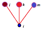
Figure 17: (Colour online) Representation of the configurations in $V_{1}$ on a Cayley tree of the order three, $i,j,k,m\in\{1,2,3\}$. For $n=1$, the number of configurations is 81.

If we take into account the 3-state Potts model associated with the Hamiltonian given in (4.18) on a Cayley tree of the order 3, we obtain the following partition equation:

$$Z^{(n)}\left(\begin{array}[]{ccc}j&k&m\\ &i&\end{array}\right) = \mathrm{e}^{A}\mathrm{e}^{B}\mathrm{e}^{C}Z^{(n)}(i,j)Z^{(n)}(i,k)Z^{(n)}(i,m),$$ (4.21)

where $A=\beta J_{nn}(\delta_{ij}+\delta_{ik}+\delta_{im}),B=\beta J_{tt}(\delta_{ijk}+\delta_{ikm}+\delta_{ijm}),C=\beta J_{pn}(\delta_{jk}+\delta_{jm}+\delta_{km})$.

Due to $i,j,k,m\in\{1,2,3\}$ there are $3^{4}=81$ different partial partition functions

$$Z^{(n)}\left(\begin{array}[]{ccc}i_{1}&i_{2}&i_{3}\\ &i_{0}&\end{array}\right).$$

Moreover, the total partition function $Z^{(n)}$ in volume $V_{n}$ is obtained as;

$$Z^{(n)}=\sum_{i_{0},i_{1},i_{2},i_{3}=1}^{3}Z^{(n)}\left(\begin{array}[]{ccc}i_{1}&i_{2}&i_{3}\\ &i_{0}&\end{array}\right).$$

However, it is reasonable to assume that the different branches are comparable, as is common in the tree models. We have only chosen five independent variables in [60] as follows;

$$z_{1}^{(n)}=Z^{(n)}\left(\begin{array}[]{ccc}1&1&1\\ &1&\end{array}\right),\quad z_{2}^{(n)}=Z^{(n)}\left(\begin{array}[]{ccc}1&1&1\\ &2&\end{array}\right),\quad z_{3}^{(n)}=Z^{(n)}\left(\begin{array}[]{ccc}2&2&2\\ &1&\end{array}\right),$$

$$\quad z_{4}^{(n)}=Z^{(n)}\left(\begin{array}[]{ccc}2&2&2\\ &2&\end{array}\right),\quad z_{5}^{(n)}=Z^{(n)}\left(\begin{array}[]{ccc}3&3&3\\ &2&\end{array}\right).$$

We investigate the relationship between the partition function on $V_{n}$ and the partition function on subsets of $V_{n-1}$ to get the recursive equations [60]. If we add the following five new variables to the equation:

$$u_{i}^{(n)}=\sqrt[3]{z_{i}^{(n)}},\ \text{for}\ i=1,2,...5,$$

after some very long and tedious calculations, we derive the corresponding recursive equations:

$$\left\{\begin{array}[]{l}u_{1}^{(n+1)}=a^{3}c\left[\sum\limits_{i=0}^{3}C_{i}^{3}\left(bu_{1}^{(n)}\right)^{3-i}+\left(2u_{2}^{(n)}\right)^{i}a^{\frac{3i(i-3)}{2}}\right],\\ u_{2}^{(n+1)}=\sum\limits_{i=0}^{3}C_{i}^{3}(u_{3}^{(n)})^{i}b^{i}\left[\sum\limits_{j=0}^{3-i}C_{j}^{3-i}\left(u_{4}^{(n)}\right)^{j}\left(u_{5}^{(n)}\right)^{3-i-j}a^{\frac{3j(j-3)}{2}}\right],\\ u_{3}^{(n+1)}=\sum\limits_{i=0}^{3}\left[\left(u_{1}^{(n)}\right)^{3-i}\left(u_{2}^{(n)}\right)^{i}(b+1)^{i}a^{\frac{3i(i-3)}{2}}\right],\\ u_{4}^{(n+1)}=a^{3}c\left[\sum\limits_{i=0}^{3}C_{i}^{3}(bu_{4}^{(n)}){}^{i}a^{\frac{3i(i-3)}{2}}\sum\limits_{j=0}^{3-i}\left(C_{j}^{3-i}\left(u_{3}^{(n)}\right)^{j}\left(u_{5}^{(n)}\right)^{3-i-j}\right)\right],\\ u_{5}^{(n+1)}=\sum\limits_{i=0}^{3}C_{i}^{3}(u_{5}^{(n)})^{i}b^{i}\left[\sum\limits_{j=0}^{3-i}C_{j}^{3-i}\left(u_{4}^{(n)}\right)^{j}\left(u_{3}^{(n)}\right)^{3-i-j}a^{\frac{3j(j-3)}{2}}\right],\end{array}\right.$$ (4.27)

where $C_{i}^{3}=\left(\begin{array}[]{c}3\\ i\end{array}\right)$. Let $\alpha=T/J_{nn}$, $\beta=-J_{pn}/J_{p}$ and $\gamma=J_{tt}/J_{nn}$. In [60], to investigate the phase diagrams, as it is a common approach in the literature, we obtained the recursive relations:

$$\left\{\begin{array}[]{l}x^{(n)}=\frac{2u_{2}^{(n)}+u_{3}^{(n)}+u_{5}^{(n)}}{u_{1}^{(n)}+u_{4}^{(n)}},y_{1}^{(n)}=\frac{u_{1}^{(n)}-u_{4}^{(n)}}{u_{1}^{(n)}+u_{4}^{(n)}},\\ y_{2}^{(n)}=\frac{u_{2}^{(n)}-u_{3}^{(n)}}{u_{1}^{(n)}+u_{4}^{(n)}},y_{3}^{(n)}=\frac{u_{2}^{(n)}-u_{5}^{(n)}}{u_{1}^{(n)}+u_{4}^{(n)}}.\end{array}\right.$$ (4.30)

If we substitute

$$u_{1} = \frac{(1+y_{1})A}{2},\quad u_{2}=\frac{(x+y_{2}+y_{3})A}{2},\quad u_{3}=\frac{(x+y_{3}-3y_{2})A}{2},$$

$$u_{4} = \frac{(1-y_{1})A}{2},\quad u_{5}=\frac{(x+y_{2}-3y_{3})A}{2},$$

where $A=u_{1}+u_{4}$, we finally obtain a system of the following recursive relations;

$$\left\{\begin{array}[]{l}x^{(n+1)}=F(x^{(n)},y_{1}^{(n)},y_{2}^{(n)},y_{3}^{(n)}),\\ y_{1}^{(n+1)}=G(x^{(n)},y_{1}^{(n)},y_{2}^{(n)},y_{3}^{(n)}),\\ y_{2}^{(n+1)}=H(x^{(n)},y_{1}^{(n)},y_{2}^{(n)},y_{3}^{(n)}),\\ y_{3}^{(n+1)}=K(x^{(n)},y_{1}^{(n)},y_{2}^{(n)},y_{3}^{(n)}).\end{array}\right.$$ (4.31)

Note that since the equations are excessively long, we do not write the complete result of the iterative system of equations (4.31) here. As a result, we recommend consulting the reference [60].

We obtain the initial conditions on $V_{1}$ under boundary conditions $\overline{\sigma}^{(n)}(V\setminus V_{n})\equiv 1$ as follows:

$$x^{(1)}=\frac{2b^{2}+a^{2}c^{2}+1}{a^{3}c^{3}b^{2}+ac},\quad y_{1}^{(1)}=\frac{a^{2}c^{2}b^{2}-1}{a^{2}c^{2}b^{2}+1},\quad y_{2}^{(1)}=\frac{b^{2}-a^{2}c^{2}}{a^{3}c^{3}b^{2}+ac},\quad y_{3}^{(1)}=\frac{a^{2}c^{2}-1}{a^{3}c^{3}b^{2}+ac}.$$

The recursive equations (4.30) show how their impact propagates along the tree.

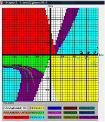
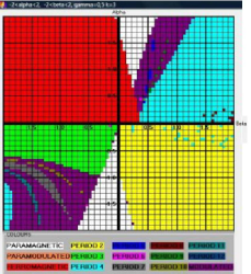
Figure 18: (Colour online) The phase diagrams of the model for $k=3$, $\gamma=0$ (left-hand) and $\gamma=0.5$ (right-hand), respectively (see [60]).

As mentioned in [60], in the simplest situation a fixed point $\left(x^{*},\,\,y_{1}^{*},\,\,y_{2}^{*},\,\,y_{3}^{*}\right)$ is reached. After a large number of iterations, if the fixed point is satisfied as $y_{1}^{*}=0,\,\,y_{2}^{*}=0,\,\,y_{3}^{*}=0$, then it corresponds to a paramagnetic phase. If $y_{1}^{*},\,\,y_{2}^{*},\,\,y_{3}^{*}\neq 0$, the phase diagram corresponds to the ferromagnetic phase. When we look at the figures 18 here, we can see that there are many different and diversified phases compared to the previous ones.

In [91], the phase diagrams of $q=5,q=6$ and $q=15$ spin states Potts models were obtained. Additionally, Gok [91] analyzed the phase diagrams of 3-state Potts model with competing for nearest neighbor, next nearest neighbor and one level triple of neighbors interactions.

Ganikhodjaev et al. [92] defined a single-trunk Cayley tree, obtained recursive equations for the model with competing interactions on the Cayley tree and for the same model on the single-trunk Cayley tree, and demonstrated how to reduce the recursion equations on the Cayley tree to the simpler recursive equations on the single-trunk Cayley tree, extended the results of [37] to the Potts model with competing interactions on a Cayley tree of arbitrary order $k$. The role of the order $k$ was clarified. They studied the differences between both types of the model on Cayley tree order 3 and order 4 and order 10. They extended the findings of [37] to the Potts model with competing interactions on a Cayley tree of any order $k$. The role of the order $k$ was described. They investigated the differences between the two types of models on Cayley tree of orders 3, 4, and 10. They demonstrated that there were six phases in the phase diagrams: ferromagnetic, paramagnetic, antiferromagnetic, period 3, antiphase, and modulated phase.

4.5 Comments and remarks

Note that the results in the section 4 are based on the studies [17, 41, 56, 60, 89, 90, 91, 92]. In this section, the system of nonlinear equations for 3-state Potts model on Cayley tree of the finite-order is derived. Secondly, the structure of the phase diagrams of given $q$-state Potts models is examined and compared and the wave vectors are plotted.

In the case $k=3$, the recursive equations are obtained. When the phase diagrams are compared with the results in the Potts model given in the previous sections, it is found that new phase regions appear in the phase diagrams. Thus, we show that the coupling constants have considerable effects on the phase diagrams.

In our works, we also see that the number of branches in the Cayley tree causes considerable changes in the phase diagrams. The phase types obtained in some regions are either completely lost or shrinking. In this case, in the regions where the modulated phases are observed, the differences are also determined by drawing the wave vectors corresponding to the magnetization in order to distinguish between the superimposed phases and the long period phases. Since more comprehensive information and findings are included in the related studies, details are not given here.

This is not rewritten here because of the length of the recursive equations. In [60], we generalized the results of Ganikhodjaev et al. [41] to the 3-state Potts model with competing NN, PNNN and two-level triple neighbor interactions on a a third-order Cayley tree. We studied the modulated phases arising from the frustration effects introduced by NN, PNNN and two-level triple neighbor interactions.

For $(x^{*},0,0,0)$, we performed the stability of the dynamical system in our previous work. However, the problem of linearization around $(x^{*},y_{1}^{*},y_{2}^{*},y_{3}^{*})$ (where at least one of $y_{1}^{*},y_{2}^{*},y_{3}^{*}$ is different from zero) is extremely difficult.

In [92], Ganikhodjaev et al. defined a single-trunk Cayley tree. By deriving the recursion equations for the same model on the single-trunk Cayley tree, they showed how to reduce the recursion equations on a Cayley tree to the simpler recursion equations on the single-trunk Cayley tree. There are many open problems to be solved using this approach.

A detailed examination of $q$-state Potts models on Cayley tree of arbitrary order has not yet been done. In order to fully understand the overlapping phase regions in modulated phases, we should investigate the Lyapunov exponents, the magnetization, and the length of wave-vectors. In addition, as the number of spins increases, it becomes more difficult for us to analyze the corresponding $q$-state Potts models. Therefore, we need new methods to dissect the $q$-state Potts models with arbitrary spin values $q$.

Remark 4.3

If there is no paramagnetic phase, then the transition between the phases and the analysis of the stability problem become a more complex issue which leads to many challenging problems. We will investigate these unresolved problems in the future.

5 The dynamical behaviors of the Ising models on chandelier networks

I have an interesting story regarding how the chandelier networks model came to be. During the days when I was focused on obtaining the phase diagrams of the lattice models on the Cayley tree as part of our project’s scope, I noticed the chandelier in our living room’s ceiling while playing on the floor with my two-year-old son. When I thought of the Cayley tree’s structure, I imagined that by duplicating the tree’s structure, a Cayley-like lattice, which was the reverse of the tree, could be identified. Thus, since that date, I have been working on the concept of chandelier network.

Take, for example, a chandelier network with $k$ bulbs suspended from the ceiling. Assume that the identical $k$ quadrants are strung on each light of the first chandelier. We get a chandelier set that looks like a semi-infinite Cayley tree in this case. We presume that the nearest lighting on the same level are linked. By computing the internal, external, and entire energies corresponding to a Hamiltonian on the chandelier network that we have established, we can analyze the themes investigated in statistical physics.

As stated in the introduction, the Cayley tree is an unrealistic lattice. Many problems in statistical physics have been studied in the Cayley tree (or Bethe lattice), because the various operations and computations on this lattice are easier to grasp than the d-dimensional $\mathbf{Z}^{\text{d}}$ lattice. Hence, the results of the Cayley tree have served as inspiration for the d-dimensional $\mathbf{Z}^{\text{d}}$ lattice.

Then, we considered a matching chandelier network, which we labelled triple, quadruple, quintuple, and so on. Furthermore, we looked at how Ising models behaved dynamically on these chandelier networks. A limited number of studies have been carried out on chandelier networks so far [75, 84, 94, 95]. Although the results are similar to those of lattice models on the Cayley tree, I believe that in the future we will be able to find more realistic results about the lattice models (Ising and Potts) defined on a chandelier network. Now, let us briefly present our findings obtained by elaboration. For more comprehensive information, we encourage the readers to consult [75, 94].

5.1 Structure of the chandelier networks

In this subsection, we are going to introduce a chandelier network with $k$ branches which is similar to a semi-infinite Cayley tree of order $k$ ($k\geqslant 3$).

In a chandelier network with $k$ branches (order), the starting vertex of the chandelier network is connected to $k$ vertices, while all the other vertices are related to $k+3$ vertices. Let $C^{k}=(V,E,i)$ be order $k$ chandelier network with a root vertex $x^{(0)}\in V$. The set of vertices in the lattice is denoted by $V$, and the set of edges is denoted by $E$. The notation $i$ represents the incidence function corresponding to each edge $e\in E$, with end points $x_{1},x_{2}\in V$. Except for the initial vertex $x^{(0)}$, each vertex has $(k+3)$ nearest neighbors belonging to $V$ as the set of vertices and the set of edges. It is obvious that the root vertex $x^{(0)}$ has $k$ nearest neighbors (see figure 19). Consider a three-lamp chandelier that hangs from a ceiling. Assume that the same three quadrants from the first chandelier were added to each bulb (see figure 19).

In this case, we get a network resembling a semi-infinite Cayley tree. We suppose that each lamp is linked to the lamps in its immediate vicinity. For $x,y\in V$, the number of edges in the shortest path from $x$ to $y$ on the chandelier network $C^{k}$ ($k>2$) is denoted by $d(x,y)$. The $0$-th level refers to the fixed vertex $x^{(0)}$, while the $n$-th level refers to the vertices in $W_{n}$. We set $|x|=d(x,x^{(0)})$, $x\in V$ for the sake of simplicity.

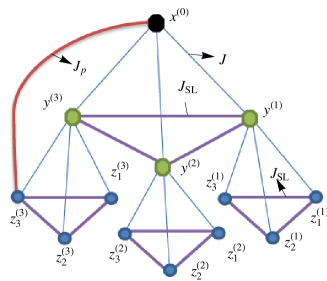
Figure 19: (Colour online) third order chandelier network of two level.

The sphere with radius $n$ on $V$ is denoted by

$$W_{n}^{(P)}=\{x\in V:d(x,x^{(0)})=n\}.$$

For example, the sphere with radius $2$ on $V$ is denoted by $W_{2}^{(P)}=\{z^{(u)}_{v}:u,v=1,2,3\}$ (see figure 19).
The ball with radius $n$ is denoted by

$$V_{n}^{(P)}=\{x\in V:d(x,x^{(0)})\leqslant n\}=\bigcup_{k=0}^{n}W_{k}^{(P)}.$$

The set of direct prolonged successors of any vertex $x\in W_{n}$ is denoted by

$$S_{k}(x)=\{y\in W_{n+1}:d(x,y)=1\}.$$

The set of the same-level neighborhoods of any vertex $x\in W_{n}$ will be denoted by

$$SL_{k}(x)=\{y\in W_{n}:d(x,y)=1\}.$$

It is clear that $|SL_{k}(x)|=2$, for all vertices $x\in W_{n}$.
Now, let us give the definitions of the neighborhood types that we considered in the chandelier networks.

Definition 5.1

1. Two vertices $x$ and $y$, $x,y\in V$ are called nearest-neighbors (NN) if there exists an edge $e\in E$ connecting them, which is denoted by $e=\langle x,y\rangle$.

2. The nearest-neighbor vertices $x,y\in V$ that are not prolonged are called same-level nearest-neighbors (SLNN) if $|x|=|y|$ and are denoted by $\widetilde{\rangle x,y\langle}$.

3. Two vertices $x,y\in V$ are called the next-nearest-neighbors (NNN) if there exists a vertex $z\in V$ such that $x,z$ and $y,z$ are NN, that is if $d(x,y)=2$.

4. The next-nearest-neighbor vertices $x\in W_{n}^{(P)}$ and $y\in W_{n+2}^{(P)}$ are called prolonged next-nearest-neighbors if $|x|\neq|y|$, $d(x,y)=2$ and is denoted by $\rangle x,y\langle$ (see figure 20).

5.2 An Ising model on triangular chandelier network (TCN)

The phase diagrams for the Ising model on a third order triangular chandelier network (TCN, shortly) are studied in [84], with competing nearest-neighbor interactions $J_{1}$, prolonged next-nearest-neighbor interactions $J_{p}$, and one-level next-nearest-neighbor quadruple interactions $J_{l_{1}}$ (figure 20).

The phase diagrams show the nonzero temperature multicritical points (Lifshitz points) as well as various modulated phases. An iterative technique similar to that found in real space renormalization group frameworks is used to carry out this study.

Let us consider the following Hamiltonian;

$$H(\sigma) = -J_{1}\sum_{\langle x,y\rangle}\sigma(x)\sigma(y)-J_{p}\sum_{\widetilde{\rangle x,y\langle}}\sigma(x)\sigma(y)$$ (5.1)

$$-J_{o}\sum_{\rangle\widehat{x,y}\langle}\sigma(x)\sigma(y)-J_{l_{1}}\sum_{\rangle x,\widehat{y,z},t\langle}\sigma(x)\sigma(y)\sigma(z)\sigma(t),$$

where we have competing nearest-neighbor $J_{1}$, prolonged next-nearest-neighbor binary interactions $J_{p}$, one-level next-nearest-neighbour binary interactions $J_{o}$, and one-level next-nearest-neighbor quadruple interactions $J_{l_{1}}$.

In [84], for some given values and signs of $J_{1},J_{p},J_{o}$ and $J_{l_{1}}$, the phase diagrams were fully determined at vanishing temperature. For typical values of $J_{l_{1}}/J_{1}$ and $J_{p}/J_{1}$ at finite temperatures, numerous interesting aspects were ovserved.

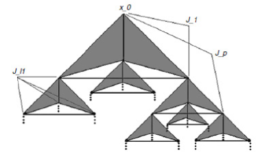
Figure 20: An infinite TCN.

5.3 The phase diagrams of an Ising model on rectangular chandelier network (RCN)

On a new kind of lattice which we called the rectangular chandelier, the authors of [75] investigated the phase diagrams of the Ising model with competing ternary and nearest-neighbor binary interactions, as well as one-level quinary interactions. Moreover, we observed the existence of multicritical Lifshitz points at non-zero temperature. The same methods can be used to obtain the phase diagrams on tetragon, pentagon, hexagon, …, and generally to understand the role of $k$ for triangular $(k=3)$ and rectangular ($k=4$) chandelier networks as in the case of a Cayley tree [62].

To plot the phase diagrams of Ising models on chandelier networks, we first derived the systems of nonlinear equations by applying the procedure in the previous sections. We investigated relevant phase diagrams in detail with the help of computer code by calculating the initial conditions (see [75, 62, 95] for details).

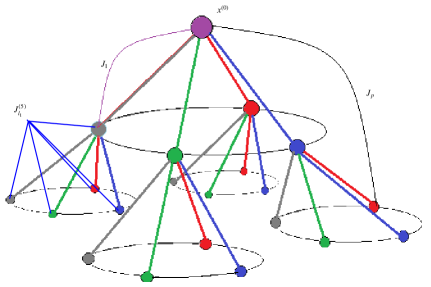
Figure 21: (Colour online) A infinite RCN. $x^{(0)}$ is the root of this lattice, and four new branches (edges) are formed from the root of the lattice. We take into account competing interactions $J_{1}$, $J_{p}$, and $J^{(5)}_{l_{1}}$, in this model.

In [95], we considered the following Hamiltonian:

$$H(\sigma)=-J_{1}\sum_{\langle x,y\rangle}\sigma(x)\sigma(y)-J_{p}\sum_{\rangle\overset{\tilde{}}{x,y}\langle}\sigma(x)\sigma(y)-J_{l_{1}}^{(5)}\sum_{\langle x,y,\overline{z},t,w\rangle}\sigma(x)\sigma(y)\sigma(z)\sigma(t)\sigma(w).$$ (5.2)

We studied the Ising model associated with Hamiltonian (5.2) on the RCN (see figure 21). The recursion relations numerically provided us the phase diagrams in $(T/J_{1}=\alpha;-J_{p}/J_{1}=\beta;J^{(5)}_{l_{1}}/J_{1}=\gamma)$ space. In addition, in [95], the authors presented the variation of the wave-vector with temperature in the modulated phase for some critical points. For the case $\beta=0.22$, we observed a distinctive feature of the phase diagram. We detected new interesting phases containing geometric figures, i.e., the phases with P5, P6, P7, and P8 in the first and second quadrants (see the figures given in 22 and 23). As can be seen in these figures, small changes in the value of $\beta$ completely change the phase diagrams.

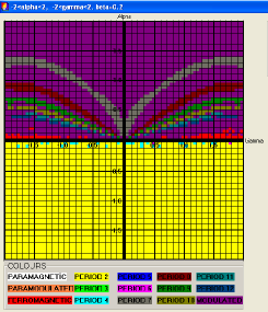
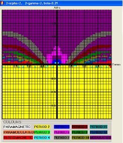
Figure 22: (Colour online) The phase diagrams of an Ising model associated with the Hamiltonian (5.2) on RCN, for $\beta=0.2$ (left-hand) and $\beta=0.21$ (right-hand) (see [95]).

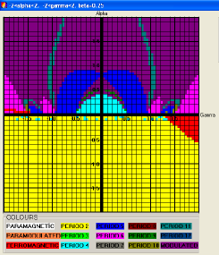
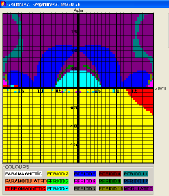
Figure 23: (Colour online) The phase diagrams of an Ising model associated with the Hamiltonian (5.2) on RCN, for $\beta=0.25$ (left-hand) and $\beta=0.26$ (right-hand) (see [95]).

Note that when the phase diagrams obtained in [95] and [75] are compared, the paramagnetic phase completely disappears in the phase diagrams obtained for the model associated with the Hamiltonian in [75].

5.4 The phase diagrams of an Ising model on pentagonal chandelier network (PCN)

We referred to the lattice in figure 24 as pentagonal chandelier network (PCN, shortly).

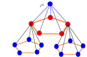
Figure 24: (Colour online) The first and second-generation branch of a PCN.

On this network shown in figure 24, we consider a Hamiltonian with spin values in $\Phi=\{-1,+1\}$ defined by

$$H(\sigma)= - J_{1}\sum_{\langle x_{1},x_{2}\rangle}\sigma(x_{1})\sigma(x_{2})-J_{p}\sum_{\rangle\widetilde{x_{1},x_{2}}\langle}\sigma(x_{1})\sigma(x_{2})$$ (5.3)

$$- J_{l_{1}}^{(6)}\sum_{\rangle x_{1},x_{2},\ldots,x_{2}\langle}\sigma(x_{1})\sigma(x_{2})\ldots\sigma(x_{6}),$$

where $J_{1},J_{p},J_{l_{1}}^{(6)}\in\mathbf{R}$ are the coupling constants. Similar to the previous models, we derived the recurrence equations corresponding to the Hamiltonian given in (5.3) as:

$$x^{\prime} = \frac{1}{a^{2}D}\left\{\sum_{r=0}^{5}C_{r}^{5}\left[b^{5-2r}c^{(-1)^{r+1}}(x-y_{2})^{5-r}(1-y_{1})^{r}+b^{-5+2r}c^{(-1)^{r}}(1+y_{1})^{5-r}(x+y_{2})^{r}\right]\right\},$$

$$y^{\prime}_{1} = \frac{1}{D}\left\{\sum_{r=0}^{5}C_{r}^{5}\left[b^{5-2r}c^{(-1)^{r}}(1+y_{1})^{5-r}(x+y_{2})^{r}-b^{-5+2r}c^{(-1)^{r+1}}(x-y_{2})^{5-r}(1-y_{1})^{r}\right]\right\},$$

$$y^{\prime}_{2} = \frac{1}{a^{2}D}\left\{\sum_{r=0}^{5}C_{r}^{5}\left[b^{5-2r}c^{(-1)^{r+1}}(x-y_{2})^{5-r}(1-y_{1})^{r}-b^{-5+2r}c^{(-1)^{r}}(1+y_{1})^{5-r}(x+y_{2})^{r}\right]\right\},$$

and

$$D(x,y_{1},y_{2}) = \sum_{r=0}^{5}C_{r}^{5}\left[b^{5-2r}c^{(-1)^{r}}(1+y_{1})^{5-r}(x+y_{2})^{r}+b^{-5+2r}c^{(-1)^{r+1}}(x-y_{2})^{5-r}(1-y_{1})^{r}\right],$$

where $a=\exp(J_{1}/T),\quad b=\exp(J_{p}/T),c=\exp(J^{(k+1)}_{l_{1}}/T)$ and $C_{r}^{5}=\left(\begin{array}[]{c}5\\ r\end{array}\right)$.

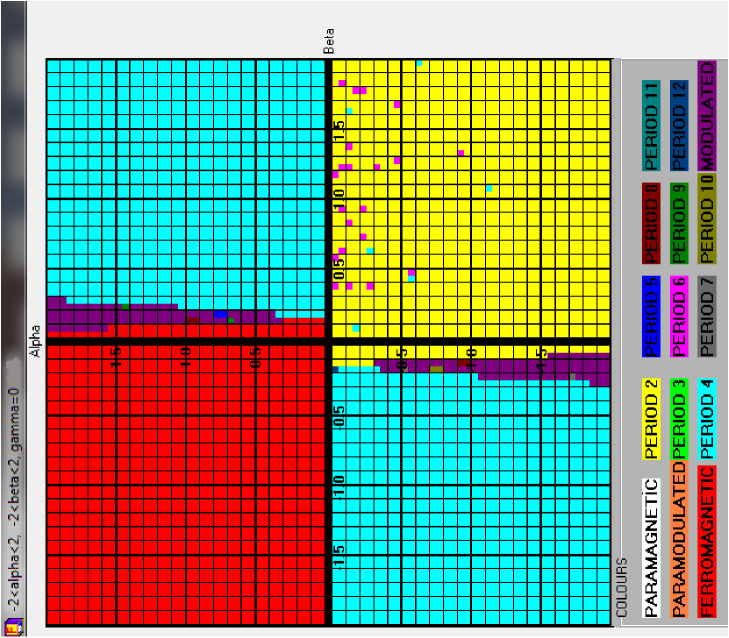
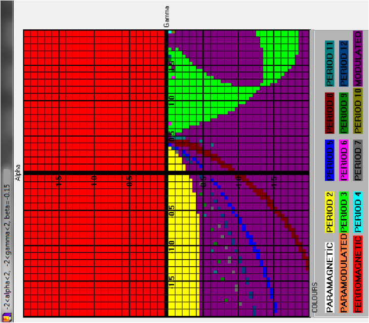
Figure 25: (Colour online) The phase diagrams of the Ising model associated to Hamiltonian (5.3) on the PCN for $(\alpha,\beta)\in[-2,2]\times[-2,2]$, $\gamma=0$ (left-hand) and $\beta=-0.15$ (right-hand).

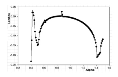
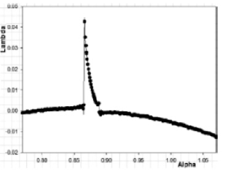
Figure 26: Lyapunov exponents of the Ising model associated with (5.3) for some values .

For the Ising model corresponding to Hamiltonian in (5.3), by using the method given in the previous sections, we can plot the phase diagrams. For example, for $\gamma=0$ and $\alpha\in[-2,2],\beta\in[-2,2]$ we have plotted the phase diagram of the Ising model associated with the Hamiltonian (5.3) in figure 25. In the diagram, P2, P4, Ferromagnetic and modulated phases mainly appear. Phases in different types of islands are also observed (see figure 25). Figure 25 (right-hand) shows a phase diagram of the Ising model associated to the Hamiltonian (5.3) for $(\alpha,\gamma)\in[-2,2]\times[-2,2]$ and $\beta=-0.15$. When figures given in 25 are compared with each other, it is seen that the phase diagrams change completely.

As known, the negative Lyapunov exponent shows that an infinitesimal perturbation in the beginning conditions has an infinitesimal effect. The negative Lyapunov exponent $\lambda$ coincides with a particular cycle phase. The positive Lyapunov exponent leads to a totally different trajectory [96]. Therefore, we calculated the Lyapunov exponents for certain critical parameter values to reveal the details in the phases.

In this way, for $\beta=0.33$ value in different intervals of $\alpha$, in figure 26, we plotted the Lyapunov exponents of the Ising model associated with the Hamiltonian given in (5.3). The figure on the right is the enlarged version of the Lyapunov exponent in the narrower range of the values. As seen in the figures, the value of the Lyapunov exponent is positive between 0.86 and 0.89. This implies that the model is chaotic in the range $(0.86,0.89)$. We look at the relevant works for details. Considering figure 25, in figure 26, we plot two variations of the Lyapunov exponent $\lambda$, $\beta=0.33$ with $\alpha\in[0.4,1.5]$ (left) and $\alpha\in[0.75,1.1]$ (right-hand). Note that the figures given in 25 are borrowed from [94].

5.5 Comments and remarks

The results in this section are based on the papers [75, 84, 94, 95, 96]. As we have seen in the relevant studies, the morphology of phase diagrams associated with a given Hamiltonian on the chandelier networks is completely different from the phase diagrams corresponding to the Ising model on the Cayley tree, if different coupling constants are added to the same Hamiltonian.

Many problems in statistical physics have lately been considered on the Cayley tree [67, 97], because other operations and computations based on this lattice are considerably simpler than the d-dimensional $\mathbf{Z}^{\text{d}}$ lattice. As a result, the Cayley tree’s results provide a source of inspiration for the d-dimensional $\mathbf{Z}^{\text{d}}$ lattice. The Ising model has relevance to physical, chemical, and biological systems [28, 98, 99]. Compared with $\mathbf{Z}^{\text{d}}$ lattice, we think that the chandelier networks are more realistic than the Cayley tree [75, 84, 94, 95, 100].

The phase diagrams for the Ising model defined on a pentagonal chandelier network with competing one-level pentagon interactions were studied by Ganikhodjaev and Rodzhan [96]. They studied the variation of wavevector with temperature in the modulated phase to detect narrow commensurate steps between incommensurate regions. They also investigated the Lyapunov exponent associated with the trajectory of the system.

5.5.1 Open problem in chandelier networks

Let us consider the following Hamiltonian

$$H(\sigma)=-J\sum\limits_{\langle x,y\rangle}{\sigma(x)\sigma(y)}-{{J}_{p}}\sum\limits_{\rangle x,y\langle}{\sigma(x)\sigma(y)}-{{J}_{SL}}\sum\limits_{\langle\widetilde{x,y}\rangle}{\sigma(x)\sigma(y)},$$ (5.4)

where the first sum encompasses all nearest neighbors, the second sum encompasses all prolonged next-nearest-neighbors, and the third sum encompasses all same-level nearest-neighbors, and $J,J_{p},J_{\text{SL}}\in\mathbf{R}$ are coupling constants (see figure 19). If $J_{\text{SL}}=0$, the Hamiltonian (5.4) coincides with the Hamiltonian of Vannimenus [2].

In this case, unlike the symmetry of a Cayley tree of arbitrary order [6], the $k$-order chandelier networks do not have symmetry when $k>3$. As a result, to derive the recursive equations associated with the Hamiltonian (5.4) for $k>3$ is much more complicated.

6 Conclusions and recommendations

I should emphasize that many of the figures given in this review paper are borrowed from the related articles.

Vannimenus [2] and Mariz et al. [3] investigated the phase diagrams of the Ising model associated with given Hamiltonian on the Cayley tree of 2th order.

Considering Vannimenus’s approach, we have determined the Lifshitz points (critical points) in the phase diagrams for certain models. The system of nonlinear equations corresponding to the Ising model was analyzed. Then, the phase diagrams of a given model were plotted and the phase diagram of Vannimenus’s model was plotted in four regions. The results and the suggestions associated with the Ising and Potts models are expressed in the discussion parts of the publications which we have accomplished, so we will not discuss them here in detail. The literature concerning the phase diagrams of the lattice models is enormous. We have tried to be as complete as possible in the bibliography, so the reader is invited to study further this interesting theory.

We have also cited some papers concerning Ising and Potts on the Cayley tree, for which many of the results presented here hold as well.

Let us summarize some of the results given in this review paper now;

1. The phase diagram of the Ising model associated with the Hamiltonian

   $$H(\sigma)=-{{J}_{p}}\sum\limits_{\langle x,y,z\rangle}{\sigma(x)\sigma(y)\sigma(z)}-J\sum\limits_{\langle x,y\rangle}{\sigma(x)\sigma(y)}$$

   was studied and the fixed points were searched to obtain the phase transition curve. The relevant phase diagram was published in the study [38].

2. The limiting behaviors of the new Ising systems with three competing interactions were studied. This phenomenon was published in the study of the corresponding phase diagrams [68]. These phase diagrams are much richer compared to the previous ones, and the Lifshitz points exhibited different properties.

3. The phase diagrams of the 3-state Potts model associated with the relevant Hamiltonian with competing nearest-neighbor, prolonged next-nearest-neighbor and two-level triple interactions were analyzed. The system of equations corresponding to the $q$-state Potts model is essentially more complicated than the similar basic equations of the Ising model [68].

4. Ganikhodjaev et al. [14] investigated the different $q$-state Potts models associated with given Hamiltonians on the Cayley tree. In this case, different and richer phase diagrams were obtained for some coupling constants and temperatures. The computer codes obtained in the study [14] were further improved by using computer programming languages such as $C^{++}$, MATLAB, MAPLE, DELPHI, VISUAL BASIC. In this context, we examined in detail the phase diagrams of the $q$-state Potts models on the Cayley tree by comparing the results obtained in the references [17, 89, 90].

5. The problem given in 5 is generalized for the Potts model, and both the phase diagrams and the linearization problem were studied. However, the Potts model encountered a longer and more complicated situation than in the investigation of these problems. The analysis of this model was examined for $k=3$.

6. We have talked about the emergence of chandelier networks. We have presented the results obtained about the lattice models described on chandelier networks so far.

7 Open problems

• When the prolonged ternary next nearest-neighbor interaction is added to the Hamiltonian, although paramagnetic phase regions for the Ising system disappear, the paramagnetic phase regions appear for the Potts model associated to similar Hamiltonian. This cannot be explained at the moment.

• On a Cayley tree of order three, Akın [101] has recently analytically analysed the recurrence equations of an Ising model with three competing interactions. He precisely described the Ising model’s paramagnetic and ferromagnetic phases. To analytically derive the phases associated with similar models on higher order Cayley trees is a difficult task.

• For both Ising and Potts models, we have obtained multiple critical points in non-zero temperatures, contrary to the works of Vannimenus [2] and Mariz et al. [3]. In the phase diagrams drawn for a model, we could perform the linearization process around the multi-critical point in the presence of the paramagnetic phase. If there is no P phase for the model, then different methods are needed to examine the stability of the system.

• It is possible to study the strange attractors of the given systems more in detail. In this context, we studied the strange attractor of an Ising system on the $k$-branch Cayley tree [63].

• Ganikhodjaev [74] studied the strange attractor in the Potts model on a Cayley tree in the presence of competing interactions. We tried to draw “Strange attractors” of Potts models for the 3rd and 4th order Cayley tree generalization of this work [74]. Relevant equations were obtained. In order to draw the graphs of these recursive equations, we need computer code studies.

• On the Cayley tree of arbitrary order, we continue to investigate Potts models with various coupling constants. The system of nonlinear equations corresponding to the Ising models was obtained as a consequence of a long calculation in the previous chapter, and new results for the Potts model associated with the Hamiltonian are expected to be investigated in the near future.

• We considered the Potts models with arbitrary spin valence ($q>3$) and came up with some interesting results. We are first referred to as phase diagrams of 4-state Potts model with mutual interaction in this manner (see [91]).

• As already mentioned, the models we have studied in this paper indicate the existence of a chaotic structure because of the diversity of the wave vectors of the phase diagrams obtained and the positive values of the Lyapunov exponents [6, 63]. We think that these calculations could be a source of inspiration for investigating more realistic models studied in physics, chemistry and other basic sciences as a result of adjusting these calculations to be more accurate with Monte Carlo and other computational techniques.

• Silva et al. [9] investigated the Ising model in the presence of an external magnetic field on a Cayley tree of any order with competitive interactions between the first-, second-, and third-nearest-neighbor interactions spins adhering to the same branch. Ganikhodjaev and Rodzhan [96] investigated phase diagrams of the Ising model on the Cayley tree with competing interactions up to the third-nearest-neighbor generation for critical variables in their paper [77]. There are numerous issues with this model. In the future, we will pursue these unsolved issues.

• Note that investigation of the stability of the Potts model is much more difficult than the stability of Ising model (see [17]). Moreover, we could not examine the quantity of Lyapunov exponent and the strange attractors associated to the Potts models in our works. We are going to investigate these concepts in the future works.

• I should note that, as far as I know, the phase diagrams of the $q$-state Potts models on $k$-order chandelier networks have not yet been studied. In [102], we investigated the reversibility of a family of linear cellular automata (LCAs) on Cayley tree of order $k$ over the field $\mathbb{F}_{p}$ and computed the measure theoretic entropy of the family of these LCAs. We will examine similar problems such as entropy and ergodic properties of these LCAs on the chandelier network. In [103], we investigated the Gibbs measures of an Ising model with competing interactions on the TCL. Gibbs measures on the other chandelier networks have not yet been explored.

Ukrainian 0

Ôàçîâi äiàãðàìè ґðàòêîâèõ ìîäåëåé íà äåðåâi Êåéëi òà ëþñòðîïîäiáíi ìåðåæi: îãëÿä [Õ. Àêèí]Õ. Àêèí${}^{\textsf{\footnotesize{\mbox{?}}}}$${}^{\textsf{\footnotesize{\mbox{?}}}}$

             
${}^{\textsf{\footnotesize 1}}$ Ìiæíàðîäíèé öåíòð òåîðåòèчíî¿ ôiçèêè iì. Àáäóñà Ñàëàìà (ICTP), Strada Costiera, 11, I - 34151 Òðiåñò, Iòàëiÿ ${}^{\textsf{\footnotesize 2}}$ Êàôåäðà ìàòåìàòèêè, ôàêóëüòåò íàóêè òà ìèñòåöòâ Õàððàíñüêîãî óíiâåðñèòåòó, 63290, Øàíëèóðôà, Òóðåччèíà

References

- [1] Baxter R. J., Exactly Solved Models in Statistical Mechanics, Academic Press, London/New York, 1982.
- [2] Vannimenus J., Z. Phys. B, 1981, 43, 141–148, doi:10.1007/BF01293605.
- [3] Mariz M., Tsalis C., Albuquerque A. L., J. Stat. Phys., 1985, 40, 577–592, doi:10.1007/BF01017186.
-
[4]
Yokoi C. S. O., Oliveira M. J., Salinas S. R.,
Phys. Rev. Lett., 1985, 54, 163–166,
doi:10.1103/PhysRevLett.54.163. - [5] Aubry S., In: The Riemann Problem, Complete Integrability and Arithmetic Applications, Springer, Berlin Heidelberg, 1982, 925, 221–245.
-
[6]
Uguz S., Ganikhodjaev N. N., Akın H., Temir S.,
Int. J. Mod. Phys. C, 2012, 23, 1250039,
doi:10.1142/S0129183112500398. - [7] Bleher P. M., Ganikhodjaev N. N., Theory Probab. Appl., 1990, 35, 216–227.
-
[8]
Coutinho S., Morgado W. A. M., Curado E. M. F., da
Silva L., Phys. Rev. B, 2006, 74, 094432,
doi:10.1103/PhysRevB.74.094432. - [9] Da Silva C.R., Coutinho S., Phys. Rev. B, 1986, 34, 7975–7985, doi:10.1103/PhysRevB.34.7975.
- [10] Marques M. C., J. Phys. A: Math. Gen., 1988, 21, 1061–1068, doi:10.1088/0305-4470/21/4/031.
- [11] Peierls R., Math. Proc. Cambridge Philos. Soc., 1936, 32, 477–481, doi:10.1017/S0305004100019174.
- [12] Pirogov S. A., Sinai Ya. G., Theor. Math. Phys., 1975, 25, 1185–1192, doi:10.1007/BF01040127.
- [13] Pirogov S. A., Sinai Ya. G., Theor. Math. Phys., 1976, 26, 39–49, doi:10.1007/BF01038255.
-
[14]
Ganikhodjaev N. N., Mukhamedov F., Pah C.H.,
Phys. Lett. A, 2008, 373, No. 1, 33–38,
doi:10.1016/j.physleta.2008.10.060. - [15] Ganikhodjaev N. N., Temir S., Akın, H., CUBO, 2005, 7, No. 3, 39–48.
- [16] Ganikhodjaev N. N., Uguz S., Physica A, 2011, 390, No. 23–24, 4160–4173, doi:10.1016/j.physa.2011.06.044.
- [17] Ganikhodjaev N. N., Temir S., Akın H., Uguz S., J. Korean Phys. Soc., 2011, 59, 2971–2979, doi:10.3938/jkps.59.2971.
- [18] Minlos R. A., Introduction to Mathematical Statistical Physics, University Lecture Series, 2000, 19.
- [19] Monroe J. L., J. Stat. Phys., 1992, 67, 1185–2000, doi:10.1007/BF01049014.
- [20] Simon B., The Statistical Mechanics of Lattice Gases, Vol. 1, Princeton University Press, Princeton, NY, 1993.
- [21] Sinai Ya. G., Theory of Phase Transitions: Rigorous Results, Pergamon, Oxford, 1982.
- [22] Takeoka Y., Berker A. N., Du R., Enoki T., Grosberg A., Kardar M., Oya T., Tanaka K., Wang G., Yu X., Tanaka T., Phys. Rev. Lett., 1999, 82, 4863–4865, doi:10.1103/PhysRevLett.82.4863.
- [23] Yang C. N., Lee T. D., Phys. Rev., 1952, 87, 410–419, doi:10.1103/PhysRev.87.410.
- [24] Yasar F., Gunduc Y., Celik T., Phys. Rev. E, 1998, 58, 4210–4212, doi:10.1103/PhysRevE.58.4210.
- [25] Monroe J. L., Phys. Rev. E, 2003, 67, 017103, doi:10.1103/PhysRevE.67.017103.
- [26] Liu Z., Luo J., Shao C., Phys. Rev. E, 2001, 64, 046134, doi:10.1103/PhysRevE.64.046134.
- [27] Schelling T. C., J. Math. Sociol., 1971 1, 143–186. doi:10.1080/0022250X.1971.9989794.
-
[28]
Georgi H.-O., Gibbs Measures and Phase Transitions, Walter
de Grugter, Berlin, 2005,
doi:10.1515/9783110250329. - [29] Inawashiro S., Thompson C. J., Honda G., J. Stat. Phys., 1983, 33, 419–436, doi:10.1007/BF01009804.
- [30] Inawashiro S., Thompson C. J., Phys. Lett. A, 1983, 97, 245–248, doi:10.1016/0375-9601(83)90758-2.
- [31] Onsager, L., Phys. Rev., 1944, 65, 117, doi:10.1103/PhysRev.65.117.
- [32] Wu F. Y., Rev. Mod. Phys., 1982, 54, No. 1, 235–268, doi:10.1103/RevModPhys.54.235.
- [33] Dobrushin R. L., Theor. Probability Appl., 1965, 10, 193–213.
- [34] Ganikhodjaev N. N., Theor. Math. Phys., 2002, 130, 419–424.
- [35] Ganikhodjaev N. N., Akın H., Temir S., Turkish J. Math., 2007, 31, 229–238.
-
[36]
Ganikhodjaev N. N., Rozikov U. A., The Abdus Salam International Center for Theoretical Physics,
Preprint IC/2004/115, Miramare-Trieste, 2004. -
[37]
Ganikhodjaev N. N., Akın H.,
Uguz S., Temir S.,
J. Stat. Mech: Theory Exp., 2011, 2011, P03025,
doi:10.1088/1742-5468/2011/03/P03025. - [38] Ganikhodjaev N. N., Akın H., Uguz S., Temir S., Phase Transitions, 2011, 84, 1045–1063, doi:10.1080/01411594.2011.579395.
- [39] Monroe J. L., Phys. Lett. A., 1994, 188, 80–84, doi:10.1016/0375-9601(94)90121-X.
- [40] Tragtenberg M. H. R., Yokoi C. S. O., Phys. Rev. E, 1995, 52, 2187–2197, doi:10.1103/PhysRevE.52.2187.
- [41] Ganikhodjaev N. N., Temir S., Akın H., J. Stat. Phys., 2009, 137, 701–715, doi:10.1007/s10955-009-9869-z.
- [42] Ganikhodjaev N. N., Rozikov U. A., Osaka J. Math., 2000, 37, 373–383.
- [43] Ganikhodjaev N. N., Theor. Math. Phys., 1990, 85, 1125–1134, doi:10.1007/BF01086840.
- [44] Ganikhodjaev N. N., Rozikov U. A., Lett. Math. Phys., 2006, 75, 99–109, doi:10.1007/s11005-005-0032-8.
- [45] Ganikhodjaev N. N., J. Math. Phys., 2004, 45, 1121–1127, doi:10.1063/1.1643194.
-
[46]
Akın H., Ganikhodjaev N. N., Uguz S., Temir S.,
Acta Phys. Pol. A, 2012, 121, 104–107,
doi:10.12693/APhysPolA.121.104. - [47] Potts R. B., Proc. Cambridge Philos. Soc., 1952, 48, 106–109, doi:10.1017/S0305004100027419.
- [48] Elliott R. J., Phys. Rev., 1961, 124, 340–345, doi:10.1103/PhysRev.124.340.
- [49] Graner F., Glazier J. A., Phys. Rev. Lett., 1992, 69, 2013–2016, doi:10.1103/PhysRevLett.69.2013.
- [50] Merks R. M. H., Glazier J. A., Physica A, 2005, 352, 113–130, doi:10.1016/j.physa.2004.12.028.
-
[51]
Ouchi N. B., Glazier J. A., Rieu J. P., Upadhyaya
A., Sawada Y., Physica A, 2003, 329, 451–458,
doi:10.1016/S0378-4371(03)00574-0. - [52] Berthod M., Kato Z., Yu S., Zerubia J., Image Vision Comput., 1996, 14, 285–295.
- [53] Won C. S., Gray R. M., Stochastic Image Processing, Kluwer Academics/Plenum Publishers, New York, 2004.
- [54] Zinati R. B. A., Codello A., J. Stat. Mech: Theory Exp., 2018, 2018, 013206, doi:10.1088/1742-5468/aa9dcc.
- [55] Akın H., Ulusoy S., Physica B, 2022, 640, 413944, doi:10.1016/j.physb.2022.413944.
-
[56]
Ganikhodjaev N. N., Mukhamedov F. M., Mendes J. F. F.,
J. Stat. Mech., 2006, 2006,
P08012, doi:10.1088/1742-5468/2006/08/P08012. -
[57]
Ganikhodjaev N. N., Rozikov U. A.,
Math. Phys. Anal. Geom., 2009, 12, 141–156,
doi:10.1007/s11040-009-9056-0. -
[58]
Ganikhodjaev N. N., Rozikov U. A., The Abdus Salam International Center for Theoretical Physics,
Preprint IC/2004/117, Miramare-Trieste, 2005. - [59] Ganikhodjaev N. N., Rozikov U. A., Theor. Math. Phys., 1997, 111, 480–486, doi:10.1007/BF02634202.
- [60] Temir S., Ganikhodjaev N. N., Uguz S., Akın H., Acta Phys. Pol. A, 2013, 123, 476–479, doi:10.12693/APhysPolA.123.476.
-
[61]
Uguz S., Ganikhodjaev N. N., Temir S., Akın H.,
AIP Conf. Proc., 2010, 1281, 2074–2077,
doi:10.1063/1.3498359. - [62] Ganikhodjaev N. N., Uguz S., Physica A, 2011, 390, 4160–4173, doi:10.1016/j.physa.2011.06.044.
-
[63]
Ganikhodjaev N. N., Akın H., Temir S., Uguz S.,
Nawi A. M.,
J. Phys. Conf. Ser., 2013, 435,
012031, doi:10.1088/1742-6596/435/1/012031. - [64] Ostilli M., Physica A, 2012, 391, 3417–3423, doi:10.1016/j.physa.2012.01.038.
- [65] Rozikov U. A., Rev. Math. Phys., 2013, 25, 1330001, doi:10.1142/S0129055X1330001X.
- [66] Rozikov U., Gibbs Measures on Cayley Trees, World scientific, Singapore, 2013.
- [67] Dang H., Weiguo Y., Zhiyan S., IEEE Trans. Inf. Theory, 2015, 61, 1640–1648, doi:10.1109/TIT.2015.2404310.
- [68] Ganikhodjaev N. N., Akın H., Uguz S., Temir S., J. Concr. Appl. Math., 2011, 9, 26–34.
- [69] Ising E., Z. Phys., 1925, 31, 253-258, doi:10.1007/BF02980577.
- [70] Peierls, R., Math. Proc. Cambridge Philos. Soc., 1936, 32, 477–481, doi:10.1017/S0305004100019174.
- [71] Akın H., Rozikov U. A., Temir S., J. Stat. Phys., 2011, 142, 314–321, doi:10.1007/s10955-010-0106-6.
- [72] Kindermann R., Snell J. L., Contemp. Math., 1980, 1, 99–112, doi:10.1090/conm/001/05.
- [73] Weidlich W., Br. J. Math. Stat. Psychol., 1971, 24, 251–266, doi:10.1111/j.2044-8317.1971.tb00470.x.
- [74] Ganikhodjaev N. N., J. Concr. Appl. Math., 2011, 9, 47–54.
- [75] Akın H., Uguz S., Temir S., AIP Conf. Proc., 2010, 1281, 607-611 (2010), doi:10.1063/1.3498550.
- [76] Yesilleten D., Berker A. N., Phys. Rev. Lett., 1997, 78, 1564–1567, doi:10.1103/PhysRevLett.78.1564.
- [77] Ganikhodjaev N., Mohd Rodzhan M. H., Malay. J. Math. Sci., 2016, 10, 167–180.
- [78] Tome T., Salinas S. R., Phys. Rev. A, 1989, 39, 2206–2213, doi:10.1103/PhysRevA.39.2206.
- [79] Moreira J. G., Salinas S. R., Phys. Rev. B, 1993, 47, 778–786, doi:10.1103/PhysRevB.47.778.
- [80] Pasquini M., Paladin G., Serva M., J. Stat. Phys., 1995, 80, 357–373, doi:10.1007/BF02178363.
- [81] Ganikhodjaev N., Mohamed Nawi A., AIP Conf. Proc., 2013, 1522, 1300–1305, doi:10.1063/1.4801280.
-
[82]
Akın H., Ganikhodjaev N. N., Temir S., Uguz S.,
Acta Phys. Pol. A, 2013, 123, 484–487,
doi:10.12693/APhysPolA.123.484. -
[83]
Saygili H., Akın H.,
Ucuncu mertebeden Cayley agaci uzerinde bir Ising modelinin faz
diyagramlari,
6. Ankara Matematik Günleri, Hacettepe Üniversitesi, 2-3 Haziran 2011, Ankara. - [84] Uguz S., Akın H., Physica A, 2010, 389, 1839, doi:10.1016/j.physa.2009.12.057.
- [85] Beaudin L., Rose-Hulman Undergrad. Math. J., 2007, 8, 13.
- [86] Beaudin L., Ellis-Monaghan J., Pangborn G., Shrock R., Discrete Math., 2010, 310, 2037–2053.
- [87] Peruggi F., di Liberto F., Monroy G., J. Phys. A: Math. Gen., 1983, 16, 811, doi:10.1088/0305-4470/16/4/018.
- [88] Peruggi F., di Liberto F., Monroy G., Physica A, 1987, 141, 151–186, doi:10.1016/0378-4371(87)90267-6.
- [89] Ganikhodjaev N. N., Temir S., Uguz S., Akın H., Applications in Physical, Biological and Financial Systems, Part 1, 2011, 117–125, doi:10.1007/978-1-4614-0231-2_9.
-
[90]
Temir S., Ganikhodjaev N. N., Akın H., Uguz S.,
AIP Conf. Proc., 2010, 1281, 2069–2073,
doi:10.1063/1.3498356. - [91] Gök G., Investigation of the phase diagrams of the Potts models with different interactions on second and third order Cayley tree (Unpublished master thesis https://tez.yok.gov.tr/No: 300063), Harran University, 2011.
-
[92]
Ganikhodjaev N., Nawi A. M., Rodzhan M. H. M.,
J. Phys. Conf. Ser., 2013, 435,
012033,
doi:10.1088/1742-6596/435/1/012033. - [93] Uguz S., Ganikhodjaev N., Dogan H., J. Korean Phys. Soc., 2015, 66, 1467–1474, doi:10.3938/jkps.66.1467.
-
[94]
Uguz S., Ganikhodjaev N. N., Akın H., Temir S.,
Acta Phys. Pol. A, 2012, 121, 114–118,
doi:10.12693/APhysPolA.121.114. - [95] Uguz S., Akın H., Chin. J. Phys., 2011, 49, 785–798.
- [96] Ganikhodjaev N., Rodzhan M. H. M., AIP Conf. Proc., 2014, 1635, 86–93, doi:10.1063/1.4903567.
- [97] Akın H., Chin. J. Phys., 2016, 54, 635–649, doi:10.1016/j.cjph.2016.07.010.
- [98] Ioffe D., Lett. Math. Phys., 1996, 37, 137–143, doi:10.1007/978-3-0348-9037-3-1.
- [99] Lebowitz J. L., J. Stat. Phys., 1977, 16, 463–476, doi:10.1007/BF01152284.
- [100] Moraal H., Physica A, 1978, 92, 305–314, doi:10.1016/0378-4371(78)90037-7.
- [101] Akın H., Condens. Matter Phys., 2021, 24, 13001, doi:10.5488/CMP.24.13001.
- [102] Akın H., Chang C. H., Int. J. Bifurcation Chaos, 2020, 30, 2050061, doi:10.1142/S0218127420500613.
- [103] Akın H., Condens. Matter Phys., 2019, 22, 23002, doi:10.5488/CMP.22.23002.
Ukrainian \adddialect\l@ukrainian0 \l@ukrainian