Quantum scar affecting the motion of three interacting particles in a circular trap

Abstract

We theoretically propose a quantum scar affecting the motion of three interacting particles in a circular trap. We numerically calculate the quantum eigenstates of the system and show that some of them are scarred by a classically unstable periodic trajectory, in the vicinity of which the classical analog exhibits chaos. The few–body scar we consider is stabilized by quantum mechanics, and we analyze it along the lines of the original quantum scarring mechanism [Heller, Phys. Rev.  Lett. 53, 1515 (1984)]. In particular, we identify towers of scarred quantum states which we fully explain in terms of the unstable classical trajectory underlying the scar. Our proposal is within experimental reach owing to very recent advances in Rydberg atom trapping.

I Introduction

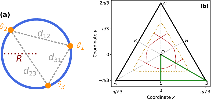
Figure 1: (a) Three particles (orange disks) interacting via a repulsive van der Waals interaction of strength $C_{6}>0$, constrained to move on a circle of radius $R$, their angular coordinates $\theta_{i}$ and distances $d_{ij}$. (b) The $(x,y)$ configuration space is the inside of the triangle defined by the points $A(-\pi/\sqrt{3},-\pi/3)$, $B(+\pi/\sqrt{3},-\pi/3)$, $C(0,2\pi/3)$. The dashed golden line limits the classically accessible region for the energy $E=7C_{6}/R^{6}$. The three dotted red lines show the three classical periodic trajectories of type $B$ for this energy. The small green triangle $OLB$ is the reduced configuration space within which quantum wavefunctions are calculated.

The thermalization of closed interacting quantum systems Polkovnikov et al. (2011) may be impeded by various mechanisms Sutherland (2004); Abanin et al. (2019) whose investigation is strongly motivated by contemporary applications Gross and Bloch (2017); Zhu et al. (2022). Indeed, slowly–thermalizing systems retain memory of their initial state over longer times Alet and Laflorencie (2018), making them useful for quantum simulation Gross and Bloch (2017) and quantum information processing Zhu et al. (2022). Atomic systems are an excellent test–bed for chaos Blümel and Reinhardt (1997); Friedrich and Wintgen (1989); Courtney et al. (1995), and techniques for the individual manipulation Browaeys and Lahaye (2020) of Rydberg atoms Saffman et al. (2010) have extended its exploration to interacting systems. A recent experiment on Rydberg atom arrays Bernien et al. (2017) has initiated the investigation of weak ergodicity breaking in many–body systems Turner et al. (2018); Serbyn et al. (2021). Systems exhibiting this phenomenon thermalize rapidly for most initial conditions, but specific initial states yield non–ergodic dynamics. This behavior is analogous to the quantum scars initially predicted Heller (1984) and observed Stein and Stöckmann (1992) in the absence of interactions, which also lead to weak ergodicity breaking Berry (1989) by impacting some (Heller, 2018, chap. 22) quantum eigenstates. Hence, it is also called ‘many–body scarring’ Jepsen et al. (2022). A similar phenomenon has been predicted in the context of the Dicke model Furuya et al. (1992), where the quantum scars are due to the collective light–matter interaction and impact many quantum eigenstates Pilatowsky-Cameo et al. (2021).

Despite the intense theoretical scrutiny Moudgalya et al. (2022), only two experiments Bernien et al. (2017); Su et al. (2022) and one explicit proposal Jepsen et al. (2022) explore many–body scarring so far Bernien et al. (2017); Jepsen et al. (2022); Su et al. (2022). In all three cases, the observed non–ergodic behavior is linked to classical physics. The experiments of Refs. Bernien et al. (2017); Su et al. (2022) both probe the PXP model Ho et al. (2019) in regimes where the classical analog system Turner et al. (2021) explores the vicinity of classically stable periodic trajectories, so that the absence of thermalization may be traced back to the classical Kolmogorov–Arnold–Moser theorem (Michailidis et al., 2020, Sec. VI). The proposal of Ref. Jepsen et al. (2022) refers to spin helices in various geometries. Their classical limit is stable Jepsen et al. (2021), and from the quantum point of view they generalize helices predicted Popkov et al. (2021) and observed Jepsen et al. (2022) in the integrable XXZ chain. Hence, the proximity of integrable models is expected to play a key role.

In this article, we propose a three–body system hosting a quantum scar which relies on the interaction between particles. It may be realized experimentally owing to very recent advances in Rydberg atom trapping Barredo et al. (2020); Cortiñas et al. (2020). It is simple enough to be fully analyzed by combining the numerical calculation of stationary states and well–established tools for the analysis of chaotic systems Gutzwiller (1990), in the spirit of Heller’s original proposal Heller (1984).

The system we consider exhibits “towers” of scarred states which are approximately evenly spaced in energy. These are a key feature of both quantum scars Heller (1991) and many–body scars Turner et al. (2018); Su et al. (2022); Moudgalya et al. (2022); Choi et al. (2019); Serbyn et al. (2021). In the present context, we explain them in terms of the classically unstable periodic trajectory causing the scar, in the spirit of Heller’s original argument (Heller, 1991, Fig. 22). The phase space dimensionality of the few–body system we consider (4, see below) matches the maximum number of independent parameters introduced so far in the variational approaches applied to the many–body PXP model and its generalizations (Michailidis et al., 2020, §III.A). In stark contrast to the many–body PXP model where approximate classical limits have to be cleverly constructed Turner et al. (2021), our few–body system affords an exact reduction to four parameters and the identification of the classical analog is straightforward.

We formulate our proposal in terms of trapped Rydberg atoms Barredo et al. (2020); Cortiñas et al. (2020). However, we expect other interacting systems with the same symmetries to exhibit similar quantum scars. We substantiate this claim in the Appendix (Sec. A.1) by identifying the quantum scar for the Hénon–Heiles (HH) potential Hénon and Heiles (1964). In particular, the scar may be probed using three dipolar particles Baranov et al. (2012).

II The considered system

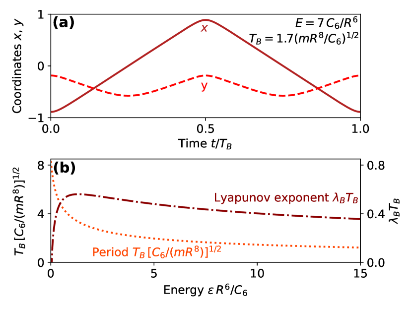
Figure 2: (a) Periodic trajectory $B$ for the energy $\epsilon=7\,C_{6}/R^{6}$, described by its coordinates $x(t)$ and $y(t)$ as a function of time $t$. (b) The period $T_{B}(\epsilon)$, and the product $\lambda_{B}\times T_{B}$ of the Lyapunov exponent and the period, for the periodic trajectory $B$ as a function of the energy $\epsilon$.

We consider three identical bosonic particles of mass $m$ in a circular trap of radius $R$. The Hamiltonian reads:

$$H=(l_{1}^{2}+l_{2}^{2}+l_{3}^{2})/(2mR^{2})+v(d_{12})+v(d_{23})+v(d_{31})\ ,$$ (1)

where $l_{i}$ is the component of the angular momentum of particle $i$ along the rotation axis, which is perpendicular to Fig. 1a. We assume that the interaction $v(d_{ij})$ between the particles $i$ and $j$ only depends on their distance $d_{ij}=2R|\sin[(\theta_{i}-\theta_{j})/2]|$. For circular Rydberg atoms whose electronic angular momenta are perpendicular to the plane, $v(d_{ij})=C_{6}/d_{ij}^{6}$ with $C_{6}>0$ (Nguyen et al., 2018, App. A).

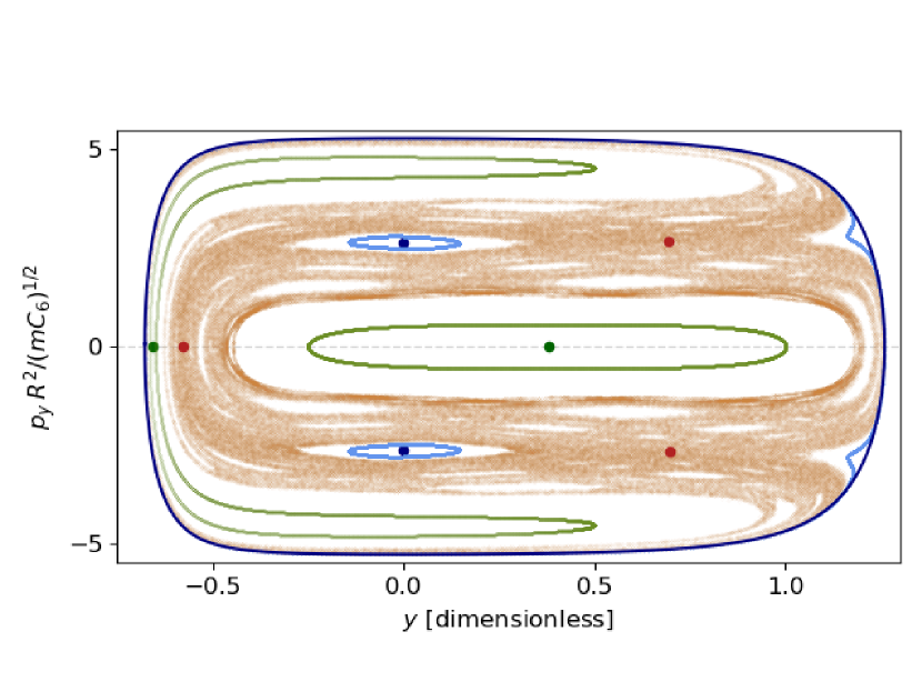
Figure 3: Classical surface of section (Lichtenberg and Lieberman, 1992, §1.2) for the Hamiltonian of Eq. (2) with $p_{z}=0$, $\epsilon=7C_{6}/R^{6}$, $x=0$, and $p_{x}\geq 0$. The dark blue dots and outer curve indicate the periodic trajectories of type $A$; the red and green dots show those of types $B$, and $C$. The closed blue and green curves show non–ergodic trajectories near $A$ and $C$. The $\sim 287,000$ thin brown dots all belong to the same ergodic trajectory. The periodic trajectories of type $B$, which yield the quantum scar, are all within the classically ergodic region.

We introduce the Jacobi coordinates (Faddeev and Merkuriev, 1993, §1.2.2) $x=[(\theta_{1}+\theta_{2})/2-\theta_{3}+\pi]/\sqrt{3}$, $y=(\theta_{2}-\theta_{1})/2-\pi/3$, $z=(\theta_{1}+\theta_{2}+\theta_{3})/3-2\pi/3$, and their conjugate momenta $p_{x}$, $p_{y}$, $p_{z}$ (which carry the unit of action). In terms of these, $H=p_{z}^{2}/(3mR^{2})+H_{\mathrm{2D}}$, where

$$H_{\mathrm{2D}}=(p_{x}^{2}+p_{y}^{2})/(4mR^{2})+V(x,y)\ .$$ (2)

Here, $V(x,y)=v(x,y)C_{6}/R^{6}$, with

$$v(x,y)=[\sin^{-6}(\pi/3+y)+\sin^{-6}(\pi/3+x\,\sqrt{3}/2-y/2)\\ +\sin^{-6}(\pi/3-x\,\sqrt{3}/2-y/2)]/64-1/9\ ,$$ (3)

energies being measured from the minimum $V(\mathbf{0})$. The free motion of the coordinate $z$ reflects the conservation of the total angular momentum $p_{z}=l_{1}+l_{2}+l_{3}$. The Hamiltonian $H$ is invariant under the point group $C_{3v}$ (Landau and Lifshitz, 1977, §93), generated by the 3–fold rotation about the axis $(x=y=0)$ and the reflection in the plane $(x=0)$.

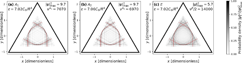
Figure 4: Probability density $|\psi(x,y)|^{2}$ of the scarred quantum eigenstate whose energy is closest to $7C_{6}/R^{6}$ in each irreducible representation $\rho=$ (a) $A_{1}$, (b) $A_{2}$, and (c) $E$. The dashed red lines show the three classically unstable periodic trajectories of type $B$ for the corresponding energy $\epsilon$. The densities are maximal near the unstable trajectories, signalling the quantum scar. The integer $\nu^{(\rho)}$ in an approximation to the index of the shown quantum state in the representation $\rho$.

III Classical physics

We first analyze the classical dynamics described by the Hamiltonian $H$. Expressing momenta, energies, and times in units of $P_{\mathrm{ref}}=(mC_{6}/R^{4})^{1/2}$, $C_{6}/R^{6}$, and $(mR^{8}/C_{6})^{1/2}$, respectively, the classical results are independent of $m$, $C_{6}$, and $R$, leading to the scaled predictions in Figs. 1–4. We choose the rotating reference frame such that $p_{z}=0$ and $z=0$. The divergence of $v(d_{ij})$ prevents the particles from crossing, so that we assume $\theta_{1}<\theta_{2}<\theta_{3}<\theta_{1}+2\pi$ at all times. Hence, the classical problem is reduced to a point moving in the 2D plane $(x,y)$ within the equilateral triangle of Fig. 1b, in the presence of the potential $V(x,y)$.

We have characterized the periodic trajectories of $V$ using our own C++ implementation of the numerical approach of Ref. Baranger et al. (1988). We find three families of periodic trajectories, existing for all energies $\epsilon>0$: we label them $A$, $B$, $C$ in analogy with the results for the HH potential Davies et al. (1992). We shall analyze them and their bifurcations in a forthcoming paper Papoular and Zumer (2023). Here, we focus on family $B$, which yields the quantum scar. For a given $\epsilon$, there are three trajectories of type $B$, due to the three–fold rotational symmetry of the potential $V$. They are represented in the $(x,y)$ plane in Fig. 1b, and the one which is symmetric about the vertical axis is shown as a function of time in Fig. 2a. They are unstable for all energies, as shown by the Lyapunov exponent $\lambda_{B}>0$ in Fig. 2b. Figure 2b shows that trajectory $B$ satisfies both conditions heralding a quantum scar: $\lambda_{B}T_{B}<2\pi$ (Heller, 2018, ch. 22), and lower values of $\lambda_{B}T_{B}$ signal stronger scarring (Ozorio de Almeida, 1988, §9.3). The unstable trajectory $B$ does not bifurcate (Ozorio de Almeida, 1988, §2.5), so that the scar strengths associated with it for all $E>0$ do not benefit from the classical enhancement due to the proximity of bifurcations Keating and Prado (2001). This sets it apart from a previous proposal involving a scar hinging on this enhancement Prado et al. (2009) so that, in stark contrast to ours, it is captured by Einstein–Brillouin–Keller quantization Zembekov et al. (1997).

In order to visualize effects beyond the linear regime, Fig. 3 shows the surface of section (Lichtenberg and Lieberman, 1992, §1.2) of $H$ for $\epsilon=7C_{6}/R^{6}$ and the conditions $x=0$, $p_{x}>0$ (allowing for a comparison with the HH potential Gustavson (1966)). It exhibits both non–ergodic regions comprising tori (Arnold, 1989, App. 8) and an ergodic region, as is typical for a non–integrable system (Bohigas et al., 1993, §1). The three fixed points corresponding to trajectories $B$ are all located in the ergodic region. This precludes their stabilization by any classical mechanism.

IV Quantum physics

We seek the eigenfunctions of $H$ in the form $\Psi_{n}(\theta_{1},\theta_{2},\theta_{3})=\psi_{n}(\mathbf{r})e^{inz}$, where $\mathbf{r}=(x,y)$ and $n=p_{z}/\hbar$. The wavefunction $\psi_{n}$ is an eigenstate of $H_{\mathrm{2D}}$ with the energy $\epsilon$. It is defined on the whole $(x,y)$ plane. Its symmetries are related to (i) angular periodicity, (ii) bosonic symmetry, and (iii) the point group $C_{3v}$.

We first discuss ${(i)}$ and ${(ii)}$. (i) The $2\pi$–periodicity of $\Psi_{n}$ in terms of $(\theta_{i})_{1\leq i\leq 3}$ yields $\psi_{n}(\mathbf{r}-\mathbf{BC})=\psi_{n}(\mathbf{r}-\mathbf{CA})=\psi_{n}(\mathbf{r}-\mathbf{AB})=\psi_{n}(\mathbf{r})e^{-i2\pi n/3}$, so that $n$ is an integer. (ii) The bosonic symmetry of $\Psi_{n}$ leads to $\psi_{n}(\mathcal{S}\mathbf{r})=+\psi_{n}(\mathbf{r})$, where $\mathcal{S}$ is the symmetry about any of the lines $(AB)$, $(BC)$ or $(CA)$ in the $(x,y)$ plane. Hence, we may restrict the configuration space to the inside of the triangle $ABC$ of Fig. 1b. Along its edges, $v(x,y)$ strongly diverges (e.g. $v\approx(y+\pi/3)^{-6}$ near $[AB]$), so that $\psi_{n}=0$ there. Combining (i) and (ii), and calling $\mathcal{R}$ the rotation of angle $2\pi/3$ about $O$, $\psi_{n}(\mathcal{R}\mathbf{r})=\psi_{n}(\mathbf{r})e^{2in\pi/3}$.

We now analyze the role of the point group $C_{3v}$. We classify the energy levels in terms of its three irreducible representations $\rho=A_{1}$, $A_{2}$, and $E$ (Landau and Lifshitz, 1977, §95). Hence, Hilbert space is split into three unconnected blocks. These may be told apart through the behavior of $\psi_{n}$ under two operations in the $(x,y)$ plane Feit et al. (1982): $\mathcal{R}$ and the reflection $\mathcal{S}_{\Delta}$ about the line $\Delta=(CL)$ (see Fig. 1b). Wavefunctions pertaining to the 1D representations $A_{1}$ or $A_{2}$ satisfy $\psi_{n}(\mathcal{R}\mathbf{r})=\psi_{n}(\mathbf{r})$, so that $n=0$ modulo 3. Under reflection, $\psi_{n}(\mathcal{S}_{\Delta}\mathbf{r})=\pm\psi_{n}$, where the $+$ and $-$ signs hold for $A_{1}$ and $A_{2}$, respectively. Wavefunctions pertaining to the 2D representation $E$ satisfy $\psi_{n}(\mathcal{R}\mathbf{r})=\exp(\pm 2i\pi/3)\psi_{n}(\mathbf{r})$, so that $n=\pm 1$ modulo 3 Brack et al. (1998). Then, exploiting time–reversal invariance (see Sec. A.2.2 in the Appendix) we may choose the two degenerate basis states to be $\psi_{n}$ and its complex conjugate $\psi_{n}^{*}$ with $\psi_{n}(\mathcal{S}_{\Delta}\mathbf{r})=\psi_{n}^{*}(\mathbf{r})$.

These symmetry considerations further reduce the configuration space to the green triangle $OLB$ of Fig. 1b. We deal with representations $A_{1}$, $A_{2}$, and $E$ separately by applying different boundary conditions on its edges (see Sec. A.2 in the Appendix). We solve the resulting stationary Schrödinger equations using the finite–element software FreeFEM Hecht (2012). The classical scaling no longer holds. Instead, the energy spectra and wavefunctions depend on the dimensionless ratio $\eta=\hbar/P_{\mathrm{ref}}=\hbar R^{2}/(mC_{6})^{1/2}$. Smaller values of $\eta$ signal deeper quasiclassical behavior: we choose $\eta=0.01$. We focus on energies $\epsilon\sim 7C_{6}/R^{6}$, which are large enough for the classical ergodic trajectory (brown dots on Fig. 3) to occupy a substantial part of phase space.

Figure 4 shows the probability density for the quantum scarred state whose energy is closest to $7C_{6}/R^{6}$ for each $\rho$. It is maximal near the three classical trajectories $B$. This signals a stabilization of trajectory $B$, whose origin is purely quantum since the unstable trajectories belong to the ergodic region of classical phase space (see Fig. 3).

V Semiclassical analysis

	$T_{B}^{(\rho)}$	$S_{B}^{(\rho)}$	$\alpha_{B}^{(\rho)}$	$k^{(\rho)}$
$A_{1}$	$T_{B}/2$	$S_{B}/2$	$\lambda_{B}T_{B}/2$	$k$
$A_{2}$	$T_{B}/2$	$S_{B}/2$	$\lambda_{B}T_{B}/2$	$k-1/2$
$E$	$2T_{B}$	$S_{B}$	$\lambda_{B}T_{B}$	$k+1/2$

Table 1: Parameters $T_{B}^{(\rho)}$, $S_{B}^{(\rho)}$, $\alpha_{B}^{(\rho)}$, $k^{(\rho)}$ for Eq. 4, depending on the irreducible representation $\rho=A_{1}$, $A_{2}$, or $E$.

For the majority of the calculated quantum states, the probability density $|\psi(x,y)|^{2}$ is unrelated to the periodic trajectories of type B. Nevertheless, for each representation, we find multiple scarred quantum states, represented by the vertical dashed lines in Fig. 5, whose energy spacing is approximately regular. This is analogous to the tower of scarred many–body states with an approximately constant energy separation found in a PXP chain Turner et al. (2018), which is a recurrent feature in theoretical analyses of weak ergodicity breaking Choi et al. (2019); Serbyn et al. (2021); Moudgalya et al. (2022). In the present context, we explain the series of scarred quantum states semiclassically. We use Gutzwiller’s trace formula (Gutzwiller, 1990, chap. 17) describing the impact of the classical periodic trajectories on the quantum density of states $n(\epsilon)$. We isolate the contribution $\Delta n_{B}^{(\rho)}$ to $n$ coming from the unstable trajectory $B$, which depends on the representation $\rho$ Robbins (1989); Lauritzen (1991):

$$(\Delta n_{B}^{(\rho)}\>2\pi\hbar/T_{B}^{(\rho)}+1)/\alpha_{B}^{(\rho)}=\\ \sum_{k=0}^{\infty}\{[S_{B}^{(\rho)}/\hbar-2\pi(k^{(\rho)}+1/2)]^{2}+(\alpha_{B}^{(\rho)}/2)^{2}\}^{-1}\ .$$ (4)

The parameters $T_{B}^{(\rho)}(\epsilon)$, $S_{B}^{(\rho)}(\epsilon)$, $\alpha_{B}^{(\rho)}(\epsilon)$, and $k^{(\rho)}$ in Eq. (4) are defined in Table 1 for each representation. They are directly related to the classical period $T_{B}(\epsilon)$ and action $S_{B}(\epsilon)=\oint\mathbf{p}\cdot d\mathbf{x}$ along one trajectory $B$, the product $\lambda_{B}(\epsilon)T_{B}(\epsilon)$, and the summation index $k$, respectively. Figure 5 shows $\Delta n_{B}^{(\rho)}(\epsilon)$ for each representation. Its maxima agree with the energies of the scarred states. Hence, the series of scarred states found in each representation reflects the multiple resonances in $n(\epsilon)$ due to the unstable trajectory $B$. The regularity in their energy spacing follows from the resonance maxima being evenly spaced in terms of the classical action, $S_{B\mathrm{max}}^{(\rho)}/\hbar=2\pi(k^{(\rho)}+1/2)$.

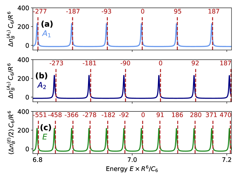
Figure 5: For each irreducible representation $\rho=$ (a) $A_{1}$, (b) $A_{2}$ and (c) $E$, the solid curve shows the semiclassical contribution $\Delta n_{B}$ (Eq. 4) to the density of states $n$ due to the periodic trajectory $B$, as a function of the energy $\epsilon$. The dashed vertical lines show the energies of the scarred quantum states, which closely match the maxima of $\Delta n_{B}$. The integers above them specify the relative state indices $\Delta\nu^{A_{1}}$, $\Delta\nu^{A_{2}}$, $\Delta\nu^{E}/2$ with respect to the index $\nu^{(\rho)}$ of the scarred states in Fig. 4.

VI Experimental prospects and outlook

We consider e.g. ${}^{87}\mathrm{Rb}$ atoms in the $50C$ circular Rydberg state Nguyen et al. (2018); Brune and Papoular (2020), for which $C_{6}/h=3\,\mathrm{GHz}\,\mathrm{\mu m}^{6}$. The value $\eta=0.01$ corresponds to $R=7\,\mu\mathrm{m}$. The ring–shaped trap may be realized optically using Laguerre–Gauss laser beams and light sheets (Amico et al., 2022, §II.C.2). The energy $\epsilon=7C_{6}/R^{6}=h\times 200\,\mathrm{kHz}$ is within experimental reach Nguyen et al. (2018). For small angular momenta, the centrifugal energy, which is proportional to $(\eta n)^{2}/3$, is negligible compared to $\epsilon$. The position of the atoms may be detected at a given time by turning on a 2D optical lattice trapping individual Rydberg atoms Nguyen et al. (2018); Anderson et al. (2011), which freezes the dynamics, followed by atomic deexcitation and site–resolved ground–state imaging Scholl et al. (2022).

Further investigation will be devoted to the stability of the quantum scar. Recent experiments Bluvstein et al. (2021); Su et al. (2022) have shown that it may be enhanced by periodically modulating the parameters. Depending on the stabilization mechanism (see e.g. Ref. Hudomal et al. (2022) or Ref. (Landau and Lifshitz, 1976, §27)), this may lead to a discrete time crystal Else et al. (2020) which is either quantum or classical.

Appendix A

The goal of this Appendix is twofold. In Section A.1, we identify novel quantum scars supported by the Hénon–Heiles Hamiltonian, and characterize them using the same semiclassical argument as in the main text. In Section A.2, for each of the three irreducible representations of the group $C_{3v}$, we derive boundary conditions defining quantum stationary states within the reduced configuration space.

A.1 Quantum scars in the Hénon–Heiles model

In this Section, we briefly describe our results, analogous to those of the main text, for the Henon–Heiles Hamiltonian Hénon and Heiles (1964) $H_{\mathrm{HH}}=(p_{x}^{2}+p_{y}^{2})/(2m)+V_{\mathrm{HH}}$, where:

$$V_{\mathrm{HH}}=m\omega_{0}^{2}(x^{2}+y^{2})/2+\alpha(x^{2}y-y^{3}/3)\ .$$ (5)

Equation 5 is written in the dimensional form of Ref. (Brack and Bhaduri, 1997, §5.6.4) which assumes that the coordinates $x$ and $y$ carry the unit of length. The quantities $p_{x}$, $p_{y}$ are their conjugate momenta, the parameters $m$ and $\omega_{0}$ denote a mass and a frequency, and the coefficient $\alpha$ sets the strength of the cubic term. If lengths, momenta, energies, and times are expressed in units of $L_{\mathrm{HH}}=m\omega_{0}^{2}/\alpha$, $P_{\mathrm{HH}}=m^{2}\omega_{0}^{3}/\alpha$, $E_{\mathrm{HH}}=m^{3}\omega_{0}^{6}/\alpha^{2}$, $T_{\mathrm{HH}}=1/\omega_{0}$, the dimensionless form matches that of Ref. Hénon and Heiles (1964). As in the main text, in terms of these units, the classical dynamics is independent of $m$, $\omega_{0}$ $\alpha$. As for quantum physics, the classical scaling no longer holds, and the energy spectra and wavefunctions depend on the dimensionless parameter $\eta_{\mathrm{HH}}=\hbar/(L_{\mathrm{HH}}P_{\mathrm{HH}})=\hbar\alpha^{2}/(m^{3}\omega_{0}^{5})$. Smaller values of $\eta_{\mathrm{HH}}$ signal deeper quasiclassical behavior.

The Hénon–Heiles potential is related to our main discussion for two reasons. First, its symmetry group is $C_{3v}$ Lauritzen (1991), which is the point group of the system analyzed in the main text. Second, expanding Eq. (3) there to third order in $x$ and $y$ near the equilibrium position $O$ shows that it reduces to Eq. 5 in the low–energy limit.

The Hénon–Heiles Hamiltonian has been extensively studied (see e.g. Ref. (Lichtenberg and Lieberman, 1992, §1.4)). Our goal in revisiting it was twofold. First, we have calibrated our codes against published results for this potential. Second, we have identified quantum scars for the Hénon–Heiles Hamiltonian which, to the best of our knowledge, are novel. At the end of the section, we point out the relevance of the Hénon-Heiles potential in relation to a broad family of systems, which includes the case of dipolar particles.

A.1.1 Calibration

We have used our codes to reproduce the known classical periodic trajectories of $H_{\mathrm{HH}}$, their periods and Lyapunov exponents Davies et al. (1992), and its surfaces of section for various energies Gustavson (1966). We have also recovered the quantum energy levels and wavefunctions, belonging to all three representations, in Refs. David and Heller (1979); Feit et al. (1982) for $\eta_{\mathrm{HH}}=1/80$ and in Ref. Brack et al. (1998) for $\eta_{\mathrm{HH}}=0.06^{2}$.

A.1.2 Quantum scars for the Hénon–Heiles potential

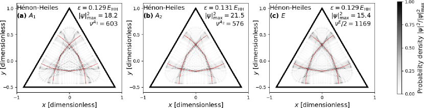
Figure 6: Probability density $|\psi_{\mathrm{(}}x,y)|^{2}$ of the scarred quantum eigenstate of the Hénon–Heiles Hamiltonian $H_{\mathrm{HH}}$ whose energy is closest to $0.13E_{\mathrm{HH}}$ in each irreducible representation (a) $A_{1}$, (b) $A_{2}$, and (c) $E$. The dashed red lines show the three classically unstable periodic trajectories of type $B$ for the corresponding energy $\epsilon$. The densities are maximal near the unstable trajectories, signaling the quantum scar. The integer $\nu^{(\rho)}$ is the index of the shown quantum state in the representation $\rho$. (This figure is the analog, for the Hénon–Heiles potential, of Fig. 4 in the main text.)

We now turn to the lower value $\eta=0.04^{2}$, so as to consider the deep quasiclassical regime. We focus on energies $\epsilon\sim 0.13\,E_{\mathrm{HH}}$: these are large enough for the ergodic region to occupy a substantial part of phase space Gustavson (1966), while remaining below the threshold energy $E_{\mathrm{HH}}/6$ above which $H_{\mathrm{HH}}$ supports trajectories that are not bound Davies et al. (1992). Figure 6 shows the probability density density for the scarred state with the energy $\epsilon$ closest to $0.13\,E_{\mathrm{HH}}$ for each representation. It is maximal near the three trajectories $B$ for the energy $\epsilon$, signaling the scar.

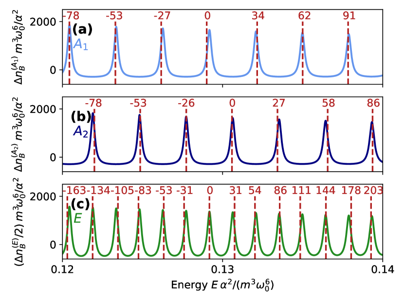
Figure 7: For each irreducible representation $\rho=$ (a) $A_{1}$, (b) $A_{2}$, and (c) $E$, the solid curve shows the semiclassical contribution $\Delta n_{B}$ to the density of states $n$ of the Hénon–Heiles potential due to the periodic trajectory $B$, as a function of the energy $\epsilon$. The dashed vertical lines show the energies of the scarred quantum states, which closely match the maxima of $\Delta n_{B}$. The integers above them specify the relative state indices $\Delta\nu^{A_{1}}$, $\Delta\nu^{A_{2}}$, $\Delta\nu^{E}/2$ with respect to the index $\nu^{(\rho)}$ of the scarred states in Fig. 6. (This figure is the analog, for the Hénon–Heiles potential, of Fig. 5 in the main text.)

In each irreducible representation $\rho=A_{1}$, $A_{2}$, and $E$, we find multiple scarred quantum states for the Hénon–Heiles potential (vertical dashed lines in Fig. 7) whose energy spacing is approximately regular, in direct analogy with the results of the main text. They may be explained using the same semiclassical argument relying on Gutzwiller’s trace formula. We isolate the contribution $\Delta n_{B}^{(\rho)}$ to the density of states $n$ for each representation $\rho$ due to the unstable trajectory $B$. Both Eq. 4 and Table I in the main text are applicable to the Hénon–Heiles potential with no change. We have calculated the required period $T_{B}$, action $S_{B}$ and Lyapunov exponent $\lambda_{B}$ characterizing the periodic trajectory $B$ in the Hénon–Heiles potential as a function of the energy $\epsilon$ using our codes. Figure 7 shows $\Delta n_{B}^{(\rho)}$ for each representation $\rho$. Just like in the main text, its maxima coincide with the energies of the scarred states. Hence, the same conclusion holds, and we may ascribe the regularity in their energy spacing to the resonance maxima being equally spaced in terms of the classical action $S_{B}$.

A.1.3 Generality of the Hénon–Heiles potential

The potential $V_{\mathrm{HH}}$ combines a 2D isotropic harmonic trap with a two–variable cubic polynomial function. Hence, it may be seen as the simplest possible 2D potential exhibiting $C_{3v}$ symmetry. The three-body Hamiltonian given by Eq. 1 in the main text reduces to it near one of its (equivalent) minima for the repulsive pair–wise interaction $v(d_{ij})=a\,d_{ij}^{-\alpha}$ regardless of the power law exponent $\alpha>0$. The presence of quantum scars in the Hénon–Heiles model leads us to expect similar scars in all of these systems. In particular, the dipole–dipole interaction Baranov et al. (2012) in the case where all three dipole moments are polarized perpendicular to the plane, corresponding to $\alpha=3$, is expected to yield the same phenomena.

A.2 Boundary conditions defining a basis of quantum stationary states

In this Section, we exploit the spatial symmetries of the point group $C_{3v}$ and time–reversal symmetry to state boundary conditions uniquely defining a basis of quantum stationary states. We state our reasoning in terms of the system considered in the main text, but it applies without change to the Hénon–Heiles Hamiltonian discussed in Sec. A.1 above.

We expect the quantum states scarred by the classically unstable periodic trajectory $B$ to exhibit an enhanced probability density along all three trajectories $B$ at a given energy (red dotted lines in Figs. 1a and 4a–c in the main text for the system discussed there, and in Figs. 6a–c in the present Appendix for the Hénon–Heiles model). Hence, the probability density for the scarred states is expected to exhibit $C_{3v}$ symmetry. Therefore, we construct a basis of quantum stationary states whose corresponding density profiles all exhibit this symmetry. This property is not automatically satisfied and requires choosing appropriate basis functions. For example, Figs. 7a and 7b in Ref. Feit et al. (1982) show probability densities corresponding to eigenstates of the Hénon–Heiles model which do not exhibit $C_{3v}$ symmetry despite the fact that the Hamiltonian does, see Sec. A.1 above.

The group $C_{3v}$ admits 3 irreducible representations, $\rho=A_{1}$, $A_{2}$, and $E$ (Landau and Lifshitz, 1977, §95). Representations $A_{1}$ and $A_{2}$ are 1D, whereas representation $E$ is 2D. For each representation, we shall formulate a boundary condition defining basis functions belonging to it. All wavefunctions $\psi(\mathbf{r})$ are normalized according to $\iint_{ABC}d^{2}r|\psi(\mathbf{r})|^{2}=1$, the integral being taken over the triangle $ABC$.

A.2.1 One–dimensional representations $A_{1}$ and $A_{2}$

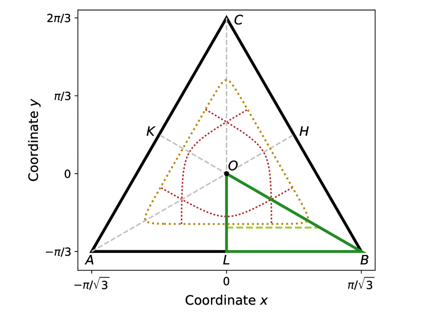
Figure 8: The black triangle $ABC$ is the classical configuration space for the Hamiltonian $H_{\mathrm{2D}}$ of the main text. The smaller green triangle $OLB$ is the reduced configuration space within which we solve for the quantum stationary states. The classically accessible region, limited by the dotted golden line, is shown for the energy $\epsilon=7C_{6}/R^{6}$. We enforce the boundary condition $\psi=0$ on the quantum wavefunctions along the horizontal dashed green line. The three classical periodic trajectories $B$ (dotted red lines) are also shown.

We first consider a 1D representation $\rho=A_{1}$ or $A_{2}$. Let $\psi$ be an eigenstate of $H_{\mathrm{2D}}$ for the energy $\epsilon$ transforming according to $\rho$. We call $\mathcal{S}_{1}$, $\mathcal{S}_{2}$, $\mathcal{S}_{3}=\mathcal{S}_{\Delta}$ the reflections about $(AH)$, $(BK)$, $(CL)$ in the $(x,y)$ plane (see Fig. 8). The wavefunction $\psi(\mathcal{S}_{i}\mathbf{r})$ is also an eigenstate of $H_{\mathrm{2D}}$ for the same energy $\epsilon$. Because $\rho$ is 1D, $\psi(\mathcal{S}_{i}\mathbf{r})=\chi_{i}\psi(\mathbf{r})$ for some complex number $\chi_{i}$. The reflections $\mathcal{S}_{i}$ satisfy $\mathcal{S}_{i}^{2}=1$, so that $\chi_{i}=\pm 1$. They also satisfy $\mathcal{S}_{2}\mathcal{S}_{1}=\mathcal{S}_{3}\mathcal{S}_{2}=\mathcal{R}$, with $\mathcal{R}$ being the rotation of angle $2\pi/3$ about the point $O$. The transformation $\mathcal{R}^{3}=1$, so that $(\chi_{1}\chi_{2})^{3}=(\chi_{2}\chi_{3})^{3}=1$. Hence, $\chi_{1}=\chi_{2}=\chi_{3}=\pm 1$.

The case $\chi_{1}=\chi_{2}=\chi_{3}=1$ leads to $\rho(\mathcal{R})=\rho(\mathcal{S}_{i})=1$, so that $\rho=A_{1}$ (Landau and Lifshitz, 1977, §95, Table 7). Then, $\psi(S_{i}\mathbf{r})=+\psi(\mathbf{r})$, leading to the boundary condition $\partial_{n}\psi=0$ along the sides $[LO]$ and $[OB]$ of the green triangle $OBL$ in Fig. 8. Combined with the condition $\psi=0$ along the side $[LB]$ derived in the main text, it defines a basis of wavefunctions $\psi$ for Representation $A_{1}$.

The case $\chi_{1}=\chi_{2}=\chi_{3}=-1$ leads to $\rho(\mathcal{R})=1$ and $\rho(\mathcal{S}_{i})=-1$, so that $\rho=A_{2}$. Then, $\psi(\mathcal{S}_{i}\mathbf{r})=-\psi(\mathbf{r})$, leading to the condition $\psi=0$ along the sides $[LO]$ and $[OB]$. Hence, imposing the Dirichlet boundary condition on the three edges of the triangle $OBL$ defines a basis of wavefunctions $\psi$ for Representation $A_{2}$.

The energy levels transforming according to the 1D representations $A_{1}$ and $A_{2}$ are non–degenerate, hence, the time–reversal invariance of $H_{\mathrm{2D}}$ allows us to choose all basis wavefunctions $\psi(\mathbf{r})$ to be real (Landau and Lifshitz, 1977, §18). Furthermore, $\psi(\mathbf{r})=\psi(\mathcal{R}^{-1}\mathbf{r})=\chi_{i}\psi(\mathcal{S}_{i}\mathbf{r})$ differ by a sign at most. Hence, the corresponding probability densities coincide, and $|\psi(\mathbf{r})|^{2}$ does exhibit $C_{3v}$ symmetry.

A.2.2 Two–dimensional representation $E$

We now turn to the 2D representation $\rho=E$. Let $\epsilon$ be a twice–degenerate energy level of $H_{\mathrm{2D}}$. The corresponding eigenspace is spanned by two complex wavefunctions, $\phi_{+}$ and $\phi_{-}$ which transform according to $\rho$:

$$\phi_{\pm}(\mathcal{R}^{-1}\mathbf{r}) =e^{\pm i2\pi/3}\phi_{\pm}(\mathbf{r})\ ,$$ (6a)

$$\phi_{\pm}(\mathcal{S}_{\Delta}\mathbf{r}) =\phi_{\mp}(\mathbf{r})\ ,$$ (6b)

where the transformations $\mathcal{R}$ and $\mathcal{S}_{\Delta}$ are defined as in Sec. A.2.1 above and the main text.

The time–reversal invariance (Landau and Lifshitz, 1977, §18) of $H_{\mathrm{2D}}$ entails that the complex–conjugate wavefunctions $\phi_{+}^{*}(\mathbf{r})$ and $\phi_{-}^{*}(\mathbf{r})$ are also eigenstates of $H_{\mathrm{2D}}$ with the same energy $\epsilon$. Complex–conjugating Eqs. (6a), accounting for normalization, and writing $(\phi_{+}^{*})^{*}=\phi_{+}$ lead to $\phi_{\pm}^{*}=e^{i\alpha}\phi_{\mp}$, where $e^{i\alpha}$ is a complex number of modulus 1. Introducing the new basis wavefunctions $\psi_{+}(\mathbf{r})=e^{i\alpha/2}\phi_{+}(\mathbf{r})$ and $\psi_{-}(\mathbf{r})=\psi_{+}^{*}(\mathbf{r})$, Eqs. (6) reduce to 2 conditions on $\psi_{+}$:

$$\psi_{+}(\mathcal{R}^{-1}\mathbf{r}) =e^{i2\pi/3}\psi_{+}(\mathbf{r})\ ,$$ (7a)

$$\psi_{+}(\mathcal{S}_{\Delta}\mathbf{r}) =\psi_{+}^{*}(\mathbf{r})\ .$$ (7b)

The probability densities $|\psi_{+}(\mathbf{r})|^{2}=|\psi_{+}(\mathcal{R}^{-1}\mathbf{r})|^{2}=|\psi_{+}(\mathcal{S}_{\Delta}\mathbf{r})|^{2}$ coincide. Hence, $|\psi_{+}(\mathbf{r})|^{2}$ exhibits $C_{3v}$ symmetry: this is the probability density plotted in Figs. 4a–c of the main text (three Rydberg atoms) and Figs. 6a–c (Hénon–Heiles model).

We seek $\psi_{+}(\mathbf{r})$ in the following form, which is more amenable to numerical computation:

$$\psi_{+}(\mathbf{r})=(x-iy)(u_{1}(\mathbf{r})+iu_{2}(\mathbf{r}))\ ,$$ (8)

where $u_{1}$ and $u_{2}$ are two real functions satisfying coupled Schrödinger equations. In Eq. (8), the factor $(x-iy)$ accounts for the fact that $\psi_{+}(\mathbf{0})=0$, like for the stationary states of the 2D isotropic harmonic oscillator carrying angular momentum (Landau and Lifshitz, 1977, §112). Equations 7 yield the boundary conditions $u_{1}=0$, $\partial_{n}u_{2}=0$ along both $[LO]$ and $[OB]$ (see Fig. 8). Combined with the condition $\psi=0$ along $[LB]$ derived in the main text, they define a basis of stationary states related to Representation $E$. For each of the twice–degenerate energy levels, $\psi_{+}(\mathbf{r})$ is given by Eq. (8) and the second basis function is $\psi_{+}^{*}(\mathbf{r})$.

A.2.3 Spatial extent of the wavefunctions

For a given energy level $\epsilon$, the spatial extent of the stationary states defined in Secs. A.2.1 and A.2.2 barely exceeds the classically accessible region (limited by the dotted golden line in Fig. 8 for the Hamiltonian $H_{\mathrm{2D}}$ of the main text and $\epsilon=7C_{6}/R^{6}$). Therefore, we restrict the region within which we solve for the wavefunctions to a part of the triangle $OLB$ which slightly exceeds this region. In other words, we enforce the condition $\psi=0$ not on $[LB]$, but on the horizontal dashed line in Fig. 8.

A.2.4 Indices of the quantum states

We order the quantum states pertaining to a given irreducible representation $\rho$ by increasing energies. This gives rise to the state index $\nu^{(\rho)}$ appearing in Figs. 4 and 5 in the main text, and Figs. 6 and 7 in the present Appendix. The irreducible representations $A_{1}$ and $A_{2}$ have dimension 1, so that, barring accidental degeneracies, the corresponding energy levels are non–degenerate. By contrast, the irreducible representation $E$ has dimension 2, meaning that each energy level is twice degenerate. For this representation, we consistently indicate one half of the state index, $\nu^{(E)}/2$, and one half of the density of states contribution $\Delta n_{B}^{(E)}/2$.

The relative level indices $\Delta\nu^{(\rho)}$ given in Fig. 5 of the main text and in Fig. 7 of this Appendix are exact. The level indices of Fig. 6, concerning the Hénon–Heiles model, are also exact. We obtain approximations to the level indices of Fig. 4 in the main text, concerning three Rydberg atoms moving along a circle, using the semiclassical appproximation to the density of states, accounting for the role of discrete spatial symmetries Lauritzen and Whelan (1995).

References

- Polkovnikov et al. (2011) A. Polkovnikov, K. Sengupta, A. Silva, and M. Vengalattore, Rev. Mod. Phys. 83, 863 (2011).
- Sutherland (2004) B. Sutherland, Beautiful models (World Scientific, 2004).
- Abanin et al. (2019) D. A. Abanin, E. Altman, I. Bloch, and M. Serbyn, Rev. Mod. Phys. 91, 021001 (2019).
- Gross and Bloch (2017) C. Gross and I. Bloch, Science 357, 995 (2017).
- Zhu et al. (2022) Q. Zhu, Z. H. Sun, M. Gong, F. Chen, Y. R. Zhang, Y. Wu, Y. Ye, C. Zha, S. Li, S. Guo, H. Qian, H. L. Huang, J. Yu, H. Deng, H. Rong, J. Lin, Y. Xu, L. Sun, C. Guo, N. Li, F. Liang, C. Z. Peng, H. Fan, X. Zhu, and J. W. Pan, Phys. Rev. Lett. 128, 160502 (2022).
- Alet and Laflorencie (2018) F. Alet and N. Laflorencie, C. R. Phys. 19, 498 (2018).
- Blümel and Reinhardt (1997) R. Blümel and W. P. Reinhardt, Chaos in atomic physics (Cambridge University Press, 1997).
- Friedrich and Wintgen (1989) H. Friedrich and D. Wintgen, Phys. Rep. 183, 37 (1989).
- Courtney et al. (1995) M. Courtney, N. Spellmeyer, H. Jiao, and D. Kleppner, Phys. Rev. A 51, 3604 (1995).
- Browaeys and Lahaye (2020) A. Browaeys and T. Lahaye, Nat. Phys. 16, 132 (2020).
- Saffman et al. (2010) M. Saffman, T. G. Walker, and K. Mølmer, Rev. Mod. Phys. 82, 2313 (2010).
- Bernien et al. (2017) H. Bernien, S. Schwartz, A. Keesling, H. Levine, A. Omran, H. Pichler, S. Choi, A. S. Zibrov, M. Endres, M. Greiner, V. Vuletić, and M. D. Lukin, Nature 551, 579 (2017).
- Turner et al. (2018) C. J. Turner, A. A. Michailidis, D. A. Abanin, M. Serbyn, and Z. Papić, Nat. Phys. 14, 745 (2018).
- Serbyn et al. (2021) M. Serbyn, D. A. Abanin, and Z. Papić, Nat. Phys. 17, 675 (2021).
- Heller (1984) E. J. Heller, Phys. Rev. Lett. 53, 1515 (1984).
- Stein and Stöckmann (1992) J. Stein and H. J. Stöckmann, Phys. Rev. Lett. 68, 2867 (1992).
- Berry (1989) M. Berry, Proc. R. Soc. Lond. A 423, 219 (1989).
- Heller (2018) E. J. Heller, The semiclassical way to physics and spectroscopy (Princeton University Press, 2018).
- Jepsen et al. (2022) P. N. Jepsen, Y. K. Lee, H. Liu, I. Dimitrova, Y. Margalit, W. W. Ho, and W. Ketterle, Nat. Phys. 18, 899 (2022).
- Furuya et al. (1992) K. Furuya, M. A. M. D. Aguiar, C. H. Lewenkopf, and M. C. Nemes, Ann. Phys. 216, 313 (1992).
- Pilatowsky-Cameo et al. (2021) S. Pilatowsky-Cameo, D. Villaseñor, M. A. Bastarrachea-Magnani, S. Lerma-Hernández, L. F. Santos, and J. G. Hirsch, Nat. Commun. 12, 852 (2021).
- Moudgalya et al. (2022) S. Moudgalya, B. A. Bernevig, and N. Regnault, Rep. Prog. Phys. 85, 086501 (2022).
- Su et al. (2022) G. Su, H. Sun, A. Hudomal, J. Desaules, Z. Zhou, B. Yang, J. C. Halimeh, Z. Yuan, Z. Papić, and J. Pan, arXiv:2201.00821 (2022).
- Ho et al. (2019) W. W. Ho, S. Choi, H. Pichler, and M. D. Lukin, Phys. Rev. Lett. 122, 040603 (2019).
- Turner et al. (2021) C. J. Turner, J. Y. Desaules, K. Bull, and Z. Papić, Phys. Rev. X 11, 021021 (2021).
- Michailidis et al. (2020) A. A. Michailidis, C. J. Turner, Z. Papić, D. A. Abanin, and M. Serbyn, Phys. Rev. X 10, 011055 (2020).
- Jepsen et al. (2021) P. N. Jepsen, W. W. Ho, J. Amato-Grill, I. Dimitrova, E. Demler, and W. Ketterle, Phys. Rev. X 11, 041054 (2021).
- Popkov et al. (2021) V. Popkov, X. Zhang, and A. Klümper, Phys. Rev. B 104, L081410 (2021).
- Barredo et al. (2020) D. Barredo, V. Lienhard, P. Scholl, S. de Léséleuc, T. Boulier, A. Browaeys, and T. Lahaye, Phys. Rev. Lett. 124, 023201 (2020).
- Cortiñas et al. (2020) R. G. Cortiñas, M. Favier, B. Ravon, P. Méhaignerie, Y. Machu, J. M. Raimond, C. Sayrin, and M. Brune, Phys. Rev. Lett. 124, 123201 (2020).
- Gutzwiller (1990) M. C. Gutzwiller, Chaos in classical and quantum mechanics (Springer, 1990).
- Heller (1991) E. J. Heller, in Les Houches Session LII (1989): chaos and quantum physics, edited by M. J. Giannoni, A. Voros, and J. Zinn-Justin (Elsevier, 1991).
- Choi et al. (2019) S. Choi, C. J. Turner, H. Pichler, W. W. Ho, A. A. Michailidis, Z. Papić, M. Serbyn, M. D. Lukin, and D. A. Abanin, Phys. Rev. Lett. 122, 220603 (2019).
- Hénon and Heiles (1964) M. Hénon and C. Heiles, Astron. J. 69, 73 (1964).
- Baranov et al. (2012) M. A. Baranov, M. Dalmonte, G. Pupillo, and P. Zoller, Chem. Rev. 112, 5012 (2012).
- Nguyen et al. (2018) T. L. Nguyen, J. M. Raimond, C. Sayrin, R. Cortiñas, T. Cantat-Moltrecht, F. Assemat, I. Dotsenko, S. Gleyzes, S. Haroche, G. Roux, T. Jolicoeur, and M. Brune, Phys. Rev. X 8, 011032 (2018).
- Lichtenberg and Lieberman (1992) A. J. Lichtenberg and M. A. Lieberman, Regular and stochastic dynamics, 2nd ed. (Springer, 1992).
- Faddeev and Merkuriev (1993) L. D. Faddeev and S. P. Merkuriev, Quantum scattering theory for several particle systems (Springer, 1993).
- Note (1) The full plane group characterizing the symmetries of is (Hahn, 2005, Part 6).
- Landau and Lifshitz (1977) L. D. Landau and E. M. Lifshitz, Quantum mechanics, non-relativistic theory (Butterworth-Heinemann, 1977).
- Baranger et al. (1988) M. Baranger, K. T. R. Davies, and J. H. Mahoney, Ann. Phys. 186, 95 (1988).
- Davies et al. (1992) K. T. R. Davies, T. E. Huston, and M. Baranger, Chaos 2, 215 (1992).
- Papoular and Zumer (2023) D. J. Papoular and B. Zumer, In preparation (2023).
- Ozorio de Almeida (1988) A. Ozorio de Almeida, Hamiltonian systems: chaos and quantization (Cambridge University Press, 1988).
- Keating and Prado (2001) J. P. Keating and S. D. Prado, Proc. R. Soc. Lond. A 457, 1855 (2001).
- Prado et al. (2009) S. D. Prado, E. Vergini, R. M. Benito, and F. Borondo, EPL 88, 40003 (2009).
- Zembekov et al. (1997) A. A. Zembekov, F. Borondo, and R. M. Benito, J. Chem. Phys. 107, 7934 (1997).
- Gustavson (1966) F. G. Gustavson, Astron. J. 71, 670 (1966).
- Arnold (1989) V. I. Arnold, Mathematical methods of classical mechanics, 2nd ed. (Springer, 1989).
- Bohigas et al. (1993) O. Bohigas, S. Tomsovic, and D. Ullmo, Phys. Rep. 223, 43 (1993).
- Feit et al. (1982) M. D. Feit, J. A. Fleck, J. A. Fleck, Jr., and A. Steiger, J. Comput. Phys. 47, 412 (1982).
- Brack et al. (1998) M. Brack, R. K. Bhaduri, J. Law, C. Maier, and M. V. N. Murthy, Chaos 5, 317 (1998).
- Hecht (2012) F. Hecht, J. Numer. Math. 20, 251 (2012).
- Robbins (1989) J. M. Robbins, Phys. Rev. A 40, 2128 (1989).
- Lauritzen (1991) B. Lauritzen, Phys. Rev. A 43, 603 (1991).
- Brune and Papoular (2020) M. Brune and D. J. Papoular, Phys. Rev. Research 2, 023014 (2020).
- Amico et al. (2022) L. Amico, D. Anderson, M. Boshier, J. Brantut, L. Kwek, A. Minguzzi, and W. von Klitzking, arXiv:2107.08561 (2022).
- Anderson et al. (2011) S. E. Anderson, K. C. Younge, and G. Raithel, Phys. Rev. Lett. 107, 263001 (2011).
- Scholl et al. (2022) P. Scholl, H. J. Williams, G. Bornet, F. Wallner, D. Barredo, L. Henriet, A. Signoles, C. Hainaut, T. Franz, S. Geier, A. Tebben, A. Salzinger, G. Zürn, T. Lahaye, M. Weidemüller, and A. Browaeys, PRX Quantum 3, 020303 (2022).
- Bluvstein et al. (2021) D. Bluvstein, A. Omran, H. Levine, A. Keesling, G. Semeghini, S. Ebadi, T. T. Wang, A. A. Michailidis, N. Maskara, W. W. Ho, S. Choi, M. Serbyn, M. Greiner, V. Vuletić, and M. D. Lukin, Science 371, 1355 (2021).
- Hudomal et al. (2022) A. Hudomal, J. Y. Desaules, B. Mukherjee, G. X. Su, J. C. Halimeh, and Z. Papić, Phys. Rev. B 106, 104302 (2022).
- Landau and Lifshitz (1976) L. D. Landau and E. M. Lifshitz, Mechanics, 3rd ed. (Butterworth-Heinemann, 1976).
- Else et al. (2020) D. V. Else, C. Monroe, C. Nayak, and N. Y. Yao, Annu. Rev. Condens. Matter Phys. 11, 467 (2020).
- Brack and Bhaduri (1997) M. Brack and R. K. Bhaduri, Semiclassical physics (Addison-Wesley, 1997).
- David and Heller (1979) M. J. David and E. J. Heller, J. Chem. Phys. 71, 3383 (1979).
- Lauritzen and Whelan (1995) B. Lauritzen and N. D. Whelan, Ann. Phys. 244, 112 (1995).
- Hahn (2005) T. Hahn, ed., International tables for crystallography volume A: space-group symmetry (Springer, 2005).