OCD: Learning to Overfit with Conditional Diffusion Models

Abstract

We present a dynamic model in which the weights are conditioned on an input sample $x$ and are learned to match those that would be obtained by finetuning a base model on $x$ and its label $y$. This mapping between an input sample and network weights is approximated by a denoising diffusion model. The diffusion model we employ focuses on modifying a single layer of the base model and is conditioned on the input, activations, and output of this layer. Since the diffusion model is stochastic in nature, multiple initializations generate different networks, forming an ensemble, which leads to further improvements. Our experiments demonstrate the wide applicability of the method for image classification, 3D reconstruction, tabular data, speech separation, and natural language processing. Our code is attached as supplementary material.

1 Introduction

Here is a simple local algorithm: For each testing pattern, (1) select the few training examples located in the vicinity of the testing pattern, (2) train a neural network with only these few examples, and (3) apply the resulting network to the testing pattern.

Bottou & Vapnik (1992)

Thirty years after the local learning method in the epigraph was introduced, it can be modernized in a few ways. First, instead of training a neural network from scratch on a handful of samples, the method can finetune, with the same samples, a base model that is pre-trained on the entire training set. The empirical success of transfer learning methods (Han et al., 2021) suggests that this would lead to an improvement.

Second, instead of retraining a neural network each time, we can learn to predict the weights of the locally-trained neural network for each set of input samples. This idea utilizes a dynamic, input-dependent architecture, also known as a hypernetwork (Ha et al., 2016).

Third, we can take the approach to an extreme and consider local regions that contain a single sample. During training, we finetune the base model for each training sample separately. In this process, which we call “overfitting”, we train on each specific sample $s=(x,y)$ from the training set, starting with the weights of the base model and obtaining a model $f_{\theta_{s}}$. We then learn a model $g$ that maps between $x$ (without the label) and the shift in the weights of $f_{\theta_{s}}$ from those of the base model. Given a test sample $x$, we apply the learned mapping $g$ to it, obtain model weights, and apply the resulting model to $x$.

The overfitted models are expected to be similar to the base model, since the samples we overfit are part of the training set of the base model. As a result, it is likely that a diffusion process would be able to generate the weights of the fine-tuned networks. Recently, diffusion models, such as DDPM (Ho et al., 2020) and DDIM (Song et al., 2020) were shown to be highly successful in generating perceptual samples (Dhariwal & Nichol, 2021b; Kong et al., 2021). Here, we employ such models as hypernetworks, i.e., as means for conditionally generating network weights.

In order to make the diffusion models suitable for predicting network weights, we make three adjustments. First, we automatically select a specific layer of the neural model and modify only this layer. This considerably reduces the size of the generated data and, in our experience, is sufficient for supporting the overfitting effect. Second, we condition the diffusion process on the input of the selected layer, its activations, and its output. Third, since the diffusion process assumes unit variance scale (Ho et al., 2020), we learn the scale of the weight modification separately.

Similarly to other diffusion processes, our hypernetwork is initialized with normal noise and different initializations lead to slightly different results. Using this feature of the diffusion model, we generate multiple models from the same instance and use the resulting ensemble technique to further improve the prediction accuracy. Our method is widely applicable, and we evaluate it across five very different domains: image classification, image synthesis, regression in tabular data, speech separation, and few-shot NLP. In all cases, the results obtained by our method improve upon the baseline model to which our method is applied. Whenever the baseline model is close to the state of the art, the leap in performance sets new state-of-the-art results.

2 Related Work

Local learning approaches perform inference with models that are focused on training samples in the vicinity of each test sample. This way, the predictions are based on what are believed to be the most relevant data points. K-nearest neighbors, for example, is a local learning method. Bottou & Vapnik (1992) have presented a simple algorithm for adjusting the capacity of the learned model locally, and discuss the advantages of such models for learning with uneven data distributions. Alpaydin & Jordan (1996) combine multiple local perceptrons in either a cooperative or a discriminative manner, and Zhang et al. (2006) combine multiple local support vector machines. These and other similar contributions rely on local neighborhoods containing multiple samples. The one-shot similarity kernel of Wolf et al. (2009) contrasts a single test sample with many training samples, but it does not finetune a model based on a single sample, as we do.

More recently, Wang et al. (2021) employ local learning to perform single-sample domain adaptation (including robustness to corruption). The adaptation is performed through an optimization process that maximizes the entropy of the prediction provided for each test sample. Our method does not require any test-time optimization and focuses (on the training samples) on improving the accuracy of the ground truth label rather than label-agnostic confidence.

Alet et al. (2021) propose a method called Tailoring that employs, like our method, meta-learning to local learning. The approach is based on applying unsupervised learning on a dataset that is created by augmenting the test sample, in a way that is related to the adaptive instance normalization of Huang & Belongie (2017). Our method does not employ any such augmentation and is based on supervised finetuning on a single sample.

Tailoring was tested on synthetic datasets with very specific structures, in a very specific unsupervised setting of CIFAR-10. Additionally, it was tested as a defense against adversarial samples, with results that fell short of the state of the art in this field. Since the empirical success obtained by Tailoring so far is limited and since there is no published code, it is not used as a baseline in our experiments.

As far as we can ascertain, all existing local learning contributions are very different from our work. No other contribution overfits samples of the training set, trains a hypernetwork for local learning, nor builds a hypernetwork based on diffusion models.

Hypernetworks (Ha et al., 2016) are neural models that generate the weights of a second primary network, which performs the actual prediction task. Since the inferred weights are multiplied by the activations of the primary network, hypernetworks are a form of multiplicative interactions (Jayakumar et al., 2020), and extend layer-specific dynamic networks, which have been used to adapt neural models to the properties of the input sample (Klein et al., 2015; Riegler et al., 2015).

Hypernetworks benefit from the knowledge-sharing ability of the weight-generating network and are therefore suited for meta-learning tasks, including few-shot learning (Bertinetto et al., 2016), continual learning (von Oswald et al., 2020), and model personalization (Shamsian et al., 2021). When there is a need to repeatedly train similar networks, predicting the weights can be more efficient than backpropagation. Hypernetworks have, therefore, been used for neural architecture search (Brock et al., 2018; Zhang et al., 2019), and hyperparameter selection (Lorraine & Duvenaud, 2018).

MEND by Mitchell et al. (2021) explores the problem of model editing for large language models, in which the model’s parameters are updated after training to incorporate new data. In our work, the goal is to predict the label of the new sample and not to update the model. Unlike MEND, our method does not employ the label of the new sample.

Diffusion models  Many of the recent generative models for images (Ho et al., 2022; Chen et al., 2020; Dhariwal & Nichol, 2021a) and speech (Kong et al., 2021; Chen et al., 2020) are based on a degenerate form of the Focker-Planck equation. Sohl-Dickstein et al. (2015) showed that complicated distributions could be learned using a simple diffusion process. The Denoising Diffusion Probabilistic Model (DDPM) of Ho et al. (2020) extends the framework and presents high-quality image synthesis. Song et al. (2020) sped up the inference time by an order of magnitude using implicit sampling with their DDIM method. Watson et al. (2021) propose a dynamic programming algorithm to find an efficient denoising schedule and San-Roman et al. (2021) apply a learned scaling adjustment to noise scheduling. Luhman & Luhman (2021) combined knowledge distillation with DDPMs.

The iterative nature of the denoising generation scheme creates an opportunity to steer the process, by considering the gradients of additional loss terms. The Iterative Latent Variable Refinement (ILVR) method Choi et al. (2021) does so for images by directing the generated image toward a low-resolution template. A similar technique was subsequently employed for voice modification Levkovitch et al. (2022). Direct conditioning is also possible: Saharia et al. (2022) generate photo-realistic text-to-image scenes by conditioning a diffusion model on text embedding; Amit et al. (2021) repeatedly condition on the input image to obtain image segmentation. In voice generation, the mel-spectrogram can be used as additional input to the denoising network Chen et al. (2020); Kong et al. (2021); Liu et al. (2021a), as can the input text for a text-to-speech diffusion model Popov et al. (2021). The conditioning we employ is of the direct type.

3 Method

Our method is based on a modified diffusion process. Denote the training dataset as $S=\{(x_{i},y_{i})\}_{i=1}^{n}$, where $x_{i}$ are the data points in the dataset $S$, and $y_{i}$ are the associated labels. First, a base model, $f_{\theta}(x)=f(x,\theta)$ is trained over the entire dataset, $S$, where $\theta$ are the learned weights of the model when trained over the entire dataset.

Next, for every training sample $s\in S$ we run fine-tuning based on that single sample to obtain the overfitted parameters (function) as $\theta_{s}$ ($f_{\theta_{s}}$).

$$\theta_{s}=\theta+\operatorname*{arg\,min}_{\Delta}(\mathcal{L}(f(x_{s},\theta+\Delta),y_{s}))\,,$$ (1)

where $\mathcal{L}$ is the loss function that is minimized in the training of the base model, $x_{s},y_{s}$ are the data point and label of sample $s$, and $\Delta$ is the weight difference obtained when finetuning the model. Finetuning is performed with three gradient descent iterations, and, as shown in our runtime analysis, is typically much less computationally demanding than the training of the base network.

The meta-learning problem we consider is the one of learning a model $g$, which maps $x$ (the input domain of sample $s$), and potentially multiple latent representations of $x$ in the context of $f_{\theta}$, collectively denoted as $I(x)$, to a vector of weight differences, such that

$$g(x,I(x))=\theta_{s}-\theta$$ (2)

where $\theta$ are the base model’s parameters trained over $S$, and $g(x,I(x))$ is a mapping function that maps the input, i.e., the $x$ part of $s$, and multiple latent representations of it, $I(x)$, to the desired shift in the model parameters.

Layer selection  Current deep neural networks can have millions or even billions of parameters. Thus, learning to modify all network parameters can be a prohibitive task. Therefore, we opt to modify, via function $g$, a single layer of $f_{\theta}$.

To select this layer, we follow Lutati & Wolf (2021) and choose the layer that presents the maximal entropy of the loss, when fixing the samples $(x,y)\in s$, and perturbing the layer’s parameters.

The layer that yields the highest entropy score when perturbed is a natural candidate for a fine-tuning algorithm, since a large entropy reflects that, near the layer’s base parameters, the surface imposed by the loss function has a large variance. Thus, a small perturbation could result in a dramatic change in loss when the perturbation is in the right direction.

Denote the perturbed weights, in which only layer $L$ is perturbed, as $\theta^{L}$. The score used for selection is

$$Score=\frac{1}{|S|}\sum_{(x,y)\in S}\text{Entropy}_{\theta_{L}}(\mathcal{L}(f(x,\theta^{L}),y))\,,$$ (3)

where $\mathcal{L}$ is the loss objective on which the function of $f_{\theta}$ is trained, and the entropy is computed over multiple draws of $\theta^{L}$. Since sampling does not involve a backpropagation computation, the process is not computationally demanding, and $10,000$ samples per each training sample $s=(x,y)$ are used.

The entropy, per each sample $s$, is computed by fitting a Gaussian Kernel Density Estimation (GKDE) (Silverman, 1986) to the obtained empirical distribution of the loss function. The layer that obtains the highest mean entropy is selected.

The conditioning signal  The latent representation, $I(x)$, has three components. Given a selected layer, $L$, we denote the input to this layer, when passing a sample $x$ to $f(x,\theta)$, as $i_{L}(x)$ and the activation of this layer as $a_{L}(x)$. We also use the output of the base function $f_{\theta}(x)$. $I(x)$ is given by the tuple

$$I(x)=[i_{L}(x),a_{L}(x),f_{\theta}(x)]$$ (4)

3.1 Diffusion Process

The goal of the diffusion process is to reconstruct $\Delta$, the difference between the fine-tuned weights $\theta_{s}$, and the base model weights, $\theta$. The process iteratively starts a random $\Omega_{T}$, with the same dimensions as $\theta_{s}$.

$$\Omega_{T}\sim\mathcal{N}(0,1)$$ (5)

Next, it iterates with $\Omega_{t}$, where $t$ is decreasing and is the diffusion step, and returns $\Omega_{0}$. After appropriate diffusion steps, $\Omega_{0}$ should be as close as possible to $\Delta$ for a given point $s$.

The diffusion error estimation network, $\epsilon_{\Omega}$ is a function of the current estimation, $\Omega_{t}$, the latent representation tuple, $I(x)$, and the diffusion timestep, $t$. The last is encoded through a positional encoding network (Vaswani et al., 2017), $PE$. All inputs, except for $\Omega_{t}$, are combined into one vector: $e=PE(t)+E_{i}(i_{L})+E_{a}(a_{L})+E_{o}(f_{\theta}(x))$, where $E_{i}$, $E_{a}$, $E_{o}$ are the encodings of the layer input, layer activations, and network output. Note that most of the components of $e$ do not change during the diffusion process, and can be computed only once. This way, the conditioning overhead is reduced to a minimum. The conditional diffusion process is depicted in Fig 1.

Training Phase  The complete training procedure of $\epsilon_{\Omega}$ is depicted in Alg. 1. The first phase is overfitting, using vanilla gradient descent over a single input-output pair, see line 1-5. The overfitting phase is not demanding, since the backpropagation is conducted only over the selected layer and a single sample.

As stated in Sec. 3.2, while regular diffusion assumes that the input has unit variance, when estimating network weights, scaling has a crucial impact. The normalization in line 6 ensures that the diffusion is trained over unit-variant input. We denote by $\Delta_{s}^{\text{norm}}$ the normalized difference between $\theta_{s}$ and the parameters $\theta$ of the base model.

Following Song et al. (2020), linear scheduling is used for the diffusion process, and $\beta_{t}$, $\alpha_{t}$, $\bar{\alpha}_{t}$, $\tilde{\beta}_{t}$ are set in line 8. A training example is then sampled:

$$\Omega_{t}=\sqrt{\bar{\alpha_{t}}}\Delta_{s}^{\text{norm}}+\sqrt{1-\bar{\alpha_{t}}}\epsilon\,,$$ (6)

where $\epsilon\sim\mathcal{N}(0,1)$ is normal noise. Since our goal is to recover the noiseless $\Delta_{s}^{\text{norm}}$, the objective is

$$||\epsilon-\epsilon_{\Omega}(\Omega_{t},(I(x),t))||\,,$$ (7)

where $\epsilon_{\Omega}$ is the diffusion error estimating model defined above. A gradient step is taken in order to optimize this objective, see line. 10.

Inference Phase  Given an unseen input $x$, $I(x)$ is computed using the base network $f(x,\theta)$ and is used for all calls to the diffusion network $\epsilon_{\Omega}$. The diffusion steps are listed in Appendix A.

Figure 1: The diffusion process. $x$ is the input of the base network, $f_{\theta}(x)$. $I(x)$ is a tuple of latent representations of $x$. $E_{i}$,$E_{a}$, and $E_{o}$ are the input, activation, and output encoders, respectively, of the selected layer that is being modified. $t$ is the diffusion step, and $\Omega_{t}$ is the current diffusion estimation.

Algorithm 1 Training Algorithm.
Input: $S$ training set, $\theta$ base network parameters, $\mathcal{L}$ the loss of the primary task, $T$ diffusion steps
Output: $\epsilon_{\Omega}$ diffusion network (incl. $E_{i}$,$E_{a}$, $E_{o}$).

1:  repeat

2:     sample $(x,y)\sim S$ and set $\theta_{s}=\theta$

3:     repeat

4:        Grad step on $\nabla\mathcal{L}(y,f_{\theta_{s}}(x))$ to update $\theta_{s}$

5:     until $\mathcal{L}(y,f_{\theta_{s}}(x))$ converges

6:     $\Delta_{s}^{\text{norm}}=\frac{\theta_{s}-\theta}{||\theta_{s}-\theta||}$

7:     $t\sim Uniform({1...T})$, $\epsilon=N(\mathbf{0},\mathbf{1})$

8:     $\beta_{t}=\frac{10^{-4}(T-t)+10^{-2}(t-1)}{T-1}$,$\alpha_{t}=1-\beta_{t}$, $\bar{\alpha_{t}}=\Pi_{k=0}^{k=t}\alpha_{k}$

9:     $\Omega_{t}=\sqrt{\bar{\alpha_{t}}}\Delta_{s}^{\text{norm}}+\sqrt{1-\bar{\alpha_{t}}}\epsilon$

10:     Grad step on $\nabla||\epsilon-\epsilon_{\Omega}(\Omega_{t},(I(x),t))||$, updating $\epsilon_{\Omega}$, $PE$ and the components of $I$

11:  until $||\epsilon-\epsilon_{\Omega}(\Omega_{t},(I(x),t))||$ converges

3.2 Scale Estimation

The Evidence Lower Bound (ELBO) used in Ho et al. (2020) assumes that the generated data has unit variance. In our case, where the generated data reflects a difference in the layer’s weights, the scale of data presents considerable variation. Naturally, shifting the weights of a network by some vector $d$ or by some scale times $d$ can create a significant difference.

We, therefore, use an MLP network $\rho(x,I(x))$ to estimate the appropriate scale factor, based on the same conditioning signal that is used for the network $\epsilon_{\Omega}$ that implements $g$ as a diffusion process. When learning network $\rho$, the following objective function is used

$$\mathcal{L}_{\text{scale}}=\sum_{s=(x,y)\in S}10\cdot log_{10}(\frac{|\rho(x,I(x))-\rho_{s}|^{2}}{\rho_{s}^{2}})\,,$$ (8)

where $\rho_{s}=||\theta_{s}-\theta||$. The use of the log scale is due to the large variance of $\Delta$. When a data point $s$ is misclassified by the base model $f\theta$, the change in the model’s weights, which results from finetuning, will be of a larger magnitude. In contrast, in the case of a sample $s$ for which the output of $f_{\theta}$ matches the label, finetuning would result in a minor update.

3.3 Architecture

Following Ho et al. (2020), the network $\epsilon_{\Omega}$ is a U-Net (Ronneberger et al., 2015). Each resolution level has residual blocks and an attention layer. The bottleneck contains two attention layers. The weights $\theta$ are arranged as a matrix, with zeros added at the edges to create a square input matrix. The output of $\epsilon_{\Omega}$ is cropped to return the original dimensions of $\theta$.

The positional encoder is composed of stacked sine and cosine encodings, following Vaswani et al. (2017). The encoders of $i_{L},a_{L}$ are both single fully-connected layers, with dimensions to match the positional embedding. The encoder of the base network’s output $f_{\theta}(x)$ depends on the output type. In the case of a classification network, where the output is a vector in $\mathbb{R^{C}}$, where $C$ is the number of classes, the encoder $E_{O}$ is a single fully-connected layer. This is also the case for our NLP experiments, which are multiclass classification experiments. In the case of image generation, the output image is first encoded using a VGG11 encoder (Simonyan & Zisserman, 2014), and then the latent representation is passed through a single fully-connected layer, again matching the dimension of the positional encoder. For speech separation, the estimated speech is first transformed to a spectogram with 1024 bins of FFT, and then encoded using the same VGG11.

4 Experiments

In all experiments, the UNet $\epsilon_{\Omega}$ has 128 channels and five downsampling layers. The positional encoding, $PE$ has dimensions of 128x128. The Adam optimizer (Kingma & Ba, 2014) is used, with a learning rate of $10^{-4}$. A linear noise schedule is used based on Song et al. (2020), and the number of diffusion steps is 10. All experiments are repeated three times to report the standard deviation (SD) of the success metrics.

In addition to the full method, we also show results for the network that overfits the test data, which serves as an upper bound that cannot be materialized without violating the train/test protocol. On some datasets we check to what extent selecting a single layer limits our results, by performing the overfitting process on all of the model weights. On all datasets, we ablate the scale component of our “Overfit with Conditional Diffusion models” (OCD) method, by estimating a fixed global scale factor $\bar{\rho}=\mathbb{E}_{s\in S}(\rho_{s})$ as the mean value of the scale factor $\rho_{s}$ over the training set. An additional ablation selects the model $f_{\theta_{s}}$ of the training sample $s$ with the closest $x$ to the test sample. This “nearest neighbor” ablation can be seen as the simplest way to implement the concept of OCD. Finally, we present an ablation that selects the layer with the second-highest layer selection score, to evaluate the significance of the selection criterion.

As an additional baseline, we employ Tent’s official implementation published by Wang et al. (2021). This baseline is employed in the vanilla classification experiments, which are similar in nature to the type of experiments Tent was previously evaluated for.

Image Classification  Results for the MNIST dataset (LeCun & Cortes, 2010) are obtained with the LeNet5 architecture (Lecun et al., 1998). The selected layer is the one next to the last fully connected layer, which, as can be seen in Appendix B has the maximal entropy among LeNet5’s layers. CIFAR10 images (Krizhevsky et al., 2009) are classified using GoogleNet (Szegedy et al., 2015). The selected layer was the last fully-connected layer, see Appendix B. For both architectures, the three encoders $E_{L_{i}},E_{L_{o}},E_{O}$ are simple fully-connected layers, with dimensions to match the number of channels in the UNet (128).

For classification experiments, we measure both the cross entropy (evaluated on the test set) and the test accuracy. As can be seen in Tab. 2, our method reduces the CE loss by a factor of 8 in comparison to the base network and there is an improvement of 0.5% in accuracy. Ablating the scale prediction, the results considerably degrade in comparison to the full method. The Nearest-Neighbor ablation yields slightly better results than the base network.

The ablation that selects an alternative layer results in performance that is similar to or slightly better than the base network. This is congruent with the small difference between fitting the selected layer and fitting all layers, which may suggest that much of the benefit of overfitting occurs in the selected layer.

On CIFAR10, our method improves classification accuracy from 92.9% to 93.7%. As in MNIST, much of the improvement is lost when the three ablations are run. In both MNIST and CIFAR, when using the ground truth to overfit a specific example, the accuracy becomes, as expected, 100%. Considering the CE loss, overfitting the entire model instead of the selected layers yields only mild improvement (below the standard deviation for MNIST). This indicates that the added improvement gained by applying our method to all layers (and not just to the selected one) may not justify the additional resources required.

Experiments were also conducted on the TinyImageNet dataset (Le & Yang, 2015). The baseline network used is the (distilled) Data efficient transformer (DeiT-B/16-D) of Touvron et al. (2022). The selected layer is the weight of the head module. Our method is able to improve on the baseline network, achieving $90.8\%$ accuracy on the test set, and falls short of the current state of the art - which requires twice as many parameters - by less than 0.5%.

The weights in the OCD hypernetwork are obtained by a diffusion process, and multiple networks can be drawn for each sample $x$. When an ensemble of five classifiers is employed, using different initializations of noise in the diffusion process, the results surpass the current state of the art, yielding $92.00\%$ ($4.7\%$ better than the baseline model, and $0.65\%$ better than the current state of the art).

Tent is not competitive with OCD on any of the image classification datasets. In the results tables, in addition to the default of 10 Tent iterations, we provide results for 1 iteration, as provided by Wang et al. (2021), and for 30 iterations, for good measure. For all benchmarks and configurations, OCD is markedly better than Tent. While Tent improves over the baseline in both MNIST and TinyImageNet, in the latter case by almost a full percent, OCD, even without an ensemble, achieves more than 2.5 percent higher accuracy.

Table 1: Performance on classification tasks. CE=Cross Entropy

	MNIST (LeNet5)		CIFAR10 (GoogleNet)
Method	Test-CE $(\downarrow)$	Accuracy %$(\uparrow)$	Test-CE $(\downarrow)$	Accuracy %$(\uparrow)$
Base network	$0.080\pm 0.009$	$99.2\pm 0.1$	$0.085\pm 0.01$	$92.85\pm 0.40$
Overfitting on test	$0.002\pm 0.0001$	$100$	$0.075\pm 0.005$	$100$
Overfitting on test (All Layers)	$0.002\pm 0.0001$	$100$	$0.073\pm 0.003$	$100$
OCD nearest neighbor ablation	$0.073\pm 0.010$	$99.3\pm 0.1$	$0.082\pm 0.02$	$93.03\pm 0.40$
OCD no scaling ablation	$0.069\pm 0.010$	$99.3\pm 0.1$	$0.084\pm 0.02$	$93.01\pm 0.35$
OCD alternative layer ablation	$0.078\pm 0.010$	$99.2\pm 0.1$	$0.084\pm 0.01$	$92.96\pm 0.27$
OCD (ours)	$\mathbf{0.010\pm 0.006}$	$\mathbf{99.7\pm 0.1}$	$\mathbf{0.080\pm 0.01}$	$\mathbf{93.68\pm 0.38}$
Base network + Tent (Wang et al. (2021), 1 iter)	$0.075\pm 0.006$	$99.4\pm 0.1$	$0.085\pm 0.03$	$92.8\pm 0.40$
Base network + Tent (Wang et al. (2021), 10 iters)	$0.073\pm 0.004$	$99.4\pm 0.1$	$0.083\pm 0.04$	$92.8\pm 0.41$
Base network + Tent (Wang et al. (2021), 30 iters)	$0.073\pm 0.004$	$99.3\pm 0.1$	$0.083\pm 0.03$	$92.8\pm 0.40$

Table 2: Classification accuracy for TinyImageNet dataset.

Method	Test-CE $(\downarrow)$	Accuracy %$(\uparrow)$
Swin L/4  (Liu et al., 2021b)	NA	$91.35$
DeiT-B/16-D (Touvron et al., 2022)	$0.71\pm 0.08$	$87.29$ $\pm 0.3$
DeiT-B/16-D + OCD	$0.65\pm 0.09$	$90.80$ $\pm 0.35$
DeiT-B/16-D + OCD, ensemble of five	$0.65\pm 0.09$	$\mathbf{92.00}$ $\pm 0.6$
DeiT-B/16-D + Tent (Wang et al. (2021), 1 iter)	$0.71\pm 0.05$	$88.15\pm 0.20$
DeiT-B/16-D + Tent (Wang et al. (2021), 10 iters)	$0.70\pm 0.02$	$88.20\pm 0.20$
DeiT-B/16-D + Tent (Wang et al. (2021), 30 iters)	$0.070\pm 0.03$	$88.20\pm 0.18$

Table 3: MSE$\pm$SD, lower is better, for the TinyNeRF network.

Method	Lego	Hotdog	Drums
Base model	$.010\pm.004$	$.012\pm.004$	$.015\pm.003$
Overfitting on test	$.006\pm.001$	$.008\pm.001$	$.009\pm.003$
OCD no scaling	$.009\pm.008$	$.012\pm.005$	$.011\pm.008$
OCD (ours)	$\mathbf{.008\pm.006}$	$\mathbf{.009\pm.004}$	$\mathbf{.010\pm.004}$

(a)	(b)	(c)

Figure 2: Sample TinyNeRF results (Lego model). More results can be found in Appendix C. (a) Base model on a test view. (b) Same test view, overfitted using the ground truth (c) OCD (ours).

Image Synthesis  We further tested our method on the image generation task of novel view synthesis, using a NeRF architecture (Mildenhall et al., 2021) and the “Synthetic-Blender” dataset. The Tiny-NeRF architecture (Murthy, 2020) employs an MLP network consisting of three fully-connected layers. The input is a 3D ray as a 5D coordinate (spatial location and viewing direction). The output is the corresponding emitted radiance. For each view, a batch of 4096 rays is computed, from which the interpolated image is synthesized.

We experimented with three objects from the dataset: Lego, Hotdog, and Drums. For each object, a different TinyNeRF base model is trained over the corresponding training set. A single overfitting example is produced by considering a batch of 4096 rays from the same viewpoint.

Based on the data in Appendix B, the first layer is selected. We, therefore, changed the layer-input encoder, $E_{i}$, such that the input image is first encoded by the VGG-11 encoder of Simonyan & Zisserman (2014) (pretrained over ImageNet-1k), followed by a fully-connected layer, to match the dimensions of UNet channels. The encoders $E_{a},E_{o}$ are simple fully-connected layers, with dimensions to match the number of channels in the UNet (128).

As can be seen in Tab. 3, our method improves the MSE by 31% for the Lego model, by 25% for Hotdog, and 16% for Drums. Without input-dependent scaling, the performance is much closer to the base network than to that of our complete method. Sample test views are shown in Fig. 2 and in Appendix C. Evidently, our method improves both image sharpness and color palette, bringing the synthesized image closer to the one obtained by overfitting the test image.

Tabular Data  Gorishniy et al. (2021) have extensively benchmarked various architectures and tabular datasets. We use their simple MLP architecture as a base network (3 Layers). We were unable to reproduce the reported transformer, since the hyperparameters are not provided, and our resources did not allow us to run a neural architecture search, as Gorishniy et al. (2021) did. We run on two of the benchmarks listed: California Housing Kelley Pace & Barry (1997) (CA), which is the first listed and has the least number of samples, and Microsoft LETOR4.0(MI) (Qin & Liu, 2013), which is the last listed and has the largest number of samples.

Based on the layer selection criterion, as depicted in Appendix B, the first layer chosen for both datasets. As can be seen in Tab. 4, for CA the base MLP model falls behind ResNet. Applying our method, the simple architecture achieves better results.

For MI when applying our method, the simple baseline achieves a record MSE of $0.743$, surpassing the current best record on this dataset, which is 0.745 (Popov et al., 2020). The ablation that removes input-dependent scaling degrades the performance of the base network, emphasizing the importance of accurate scaling per sample.

Table 4: Tabular benchmarks. $MSE\pm SD$, lower is better.

Method	CA	MI
MLP	$0.4990\pm 0.0030$	$0.7470\pm.0004$
ResNet	$0.4860\pm 0.0030$	$0.7480\pm.0003$
Overfit MLP on test	$0.4750\pm.0020$	$0.7410\pm.0003$
OCD + MLP no scale	$0.5000\pm.0030$	$0.7490\pm.0006$
OCD + MLP (ours)	$\mathbf{0.4800\pm.0020}$	$\mathbf{0.7430\pm.0004}$

Table 5: Audio separation. DM: Dynamic Mixing

Method	SI-SDRi[dB]($\uparrow$)
SepIt (Lutati et al., 2022)	$13.2\pm 0.2$
Baseline (Dovrat et al., 2021)	$12.7\pm 0.1$
Overfit baseline on test	$13.5\pm 0.1$
Baseline + OCD no scale	$12.8\pm 0.3$
Baseline + OCD (ours)	$\mathbf{13.4\pm 0.1}$
Baseline + OCD + DM (ours)	$\mathbf{13.9\pm 0.1}$

Table 6: Accuracy for few-shot NLP classification with 8 samples per class.

Method	SST-5	AmazonCF	CR	Emotion	Enron	Mean
T-few 3B (Liu et al., 2022)	$\mathbf{55.0}$	$19.0$	$92.1$	$\mathbf{57.4}$	$\mathbf{93.1}$	$63.3$
SetFit (Tunstall et al., 2022)	$43.6$	$40.3$	$88.5$	$48.8$	$90.1$	$62.2$
SetFit + OCD	$47.8$	$41.0$	$90.5$	$50.2$	$92.2$	${64.3}$
Mean of 5 OCD instances	$47.9$	$41.0$	$90.3$	$50.2$	$92.3$	${64.3}$
Ensemble of SetFit + OCD	$48.6$	$\mathbf{41.2}$	$\mathbf{91.2}$	$50.5$	$92.7$	$\mathbf{64.8}$

Speech Separation  To tackle the task of single microphone speech separation of multiple speakers, Nachmani et al. (2020) introduce the Gated-LSTM architecture with MulCat block and Dovrat et al. (2021) introduced a permutation-invariant loss based on the Hungarian matching algorithm, using the same architecture. Lutati et al. (2022) further improved results for this architecture, by employing an iterative method based on a theoretical upper bound, achieving state-of-the-art results.

The same backbone and Hungarian-method loss are used in our experiments, which run on the Libri5Mix dataset without augmentations, measuring the SI-SDRi score. The selected layer was the projection layer of the last MulCat block (Appendix B). The output of the Gated-LSTM is the separated sounds, and to encode it, we apply the audio encoding described in Sec. 3.3 to each output channel separately and concatenate before applying the linear projection to $\mathbb{R}^{128}$.

As can be seen in Tab. 6, applying our diffusion model over the Gated-LSTM model, we achieve $13.9dB$, surpassing current state-of-the-art results and approaching the results obtained by overfitting on the test data. The ablation that removes input-dependent scaling is much closer in performance to the base network than to our complete method.

Prompt-free Few-Shot NLP Classification  Recent few-shot methods have achieved impressive results in label-scarce settings. However, they are difficult to employ, since they require language models with billions of parameters and hand-crafted prompts. Very recently, Tunstall et al. (2022) introduced a lean hypernetwork architecture, named SetFit, for finetuning a pretrained sentence transformer over a small dataset (8 examples per class), and then employing logistic regression over the corresponding embedding. In our experiments, we apply OCD to the last linear layer of the SetFIT sentence transformer. The U-Net has 64 channels, with 5 downsample layers. The size of the last linear layer is $768x768$. $I(x)\in\mathbb{R}^{768x1}$ is the embedding of the Sentence Transformer.

As can be seen in Tab. 6 using OCD and this lean architecture (with 110M parameters) outperforms, on average, the state-of-the-art model of Liu et al. (2022), which has 3B parameters. The mean performance across the datasets is improved by 1.0% over the state-of-the-art and by 2.1% over the SetFIT model we build upon. Recall that since the weights in the OCD hypernetworks are obtained by a diffusion process, one can draw multiple networks for each sample $x$. The variability that arises from the random initialization of the diffusion process allows us to use an ensemble. As can be seen in Tab. 6, when applying an ensemble of five inferences, the results of OCD further improve by 0.4% (on average) to a gap of 1.5% over the state-of-the-art.

Interestingly, when testing the average network weights of the 5 networks, the accuracy is virtually identical to that obtained with a single OCD network. However, there is some reduction in Cross-Entropy for the mean network, see Appendix D).

Runtime  Tab. 7 lists the measured runtime with and without OCD for both training and inference, on the low-end Nvidia RTX2060 GPU on which all experiments were run. Since overfitting each sample includes only 3 gradient descent steps over a single layer, most of the data collection results are shorter than the training time of the base model, with the exception of LeNet5 training that used a batch size of 16 versus batch size of 1 in the overfitting stage. Training the diffusion model is slower in most experiments than training the base model, except for the speech model, in which training the base model is lengthy.

The inference overhead is almost constant across the six models, since it consists of running the UNet $\epsilon_{\Omega}$ ten times. The inference overhead due to a U-Net forward pass is 27[ms] (there are ten such passes, one per diffusion step). In absolute terms, the overhead incurred by OCD, even on a very modest GPU, is only a quarter of a second, while the results improve substantially. We note that the same $\epsilon_{\Omega}$ is used for all experiments, padding the actual weight matrix, which induces an unnecessary computational cost in the case of small networks.

Table 7: Runtime on a low-end Nvidia RTX2060GPU. Training includes the base model training, the collection of data for OCD by overfitting each sample in the training set, and the training of the diffusion model. The main overhead between the base model and the OCD one during inference is a result of running the UNet of the diffusion process for ten iterations.

	Training[hrs]			Inference[ms]
Architecture	Base	Overfit	Diffusion	Base	OCD
LeNet5	0.5	1.0	6.0	15	288
GoogleNet	2.5	1.0	5.0	20	298
TinyNeRF	1.1	0.2	5.2	230	510
MLP	1.2	0.1	6.2	75	355
Gated-LSTM	30	2.5	6.8	450	730
SetFit	0.2	0.1	5.1	125	401

5 Conclusions

We present what is, as far as we can ascertain, the first diffusion-based hypernetwork, and show that independently learning the scale is required for obtaining the best performance. The hypernetwork is studied in the specific context of local learning, in which a dynamic model is conditioned on a single input sample.

The training samples for the hypernetwork are collected by finetuning a model on each specific sample from the training set used by the base model. By construction, this is only slightly more demanding than fitting the base model on the training set. More limiting is the size of the output of the hypernetwork, which for modern networks can be larger than the output dimensions of other diffusion processes. We, therefore, focus on a single layer, which is selected as the one most affected by weight perturbations.

We tested our method extensively, tackling a very diverse set of tasks with the same set of hyperparameters. We are yet to find a single dataset or architecture on which our OCD method does not significantly improve the results of the baseline architecture.

Appendix A The inference time algorithm

The steps of the inference algorithm are listed on Alg. 2.

Algorithm 2 Inference Algorithm.
Input: $x$ input sample, $\theta$ the parameters of the base network, $\epsilon_{\Omega}$ diffusion network, T diffusion steps.
Output: $g(x,I(x))$ estimated normalized ($\theta_{s}-\theta$) for $s$ associates with $x$.

1:  $t=T$

2:  $\epsilon=N(\mathbf{0},\mathbf{1})$

3:  while $t\geq 0$ do

4:     $\beta_{t}=\frac{10^{-4}(T-t)+10^{-2}(t-1)}{T-1}$, $\alpha_{t}=1-\beta_{t}$, $\bar{\alpha_{t}}=\Pi_{k=0}^{k=t}\alpha_{k}$, $\tilde{\beta_{t}}=\frac{1-\bar{\alpha_{t-1}}}{1-\bar{\alpha_{t}}}\beta_{t}$

5:     $\Omega_{t-1}=\frac{\Omega_{t}-\frac{1-\alpha_{t}}{\sqrt{1-\bar{\alpha_{t}}}}\epsilon_{\Omega}(\Omega_{t},I(x),t)}{\sqrt{\alpha_{t}}}+\mathbf{1}_{t>1}\sqrt{\tilde{\beta_{t}}}$

6:     $t=t-1$

7:  end while

8:  return $\Omega_{0}$

Appendix B Layer selection plots

Fig. 3 depicts the layer selection criterion for various experiments.

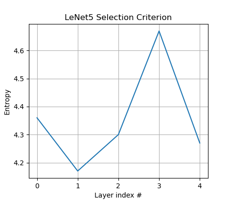
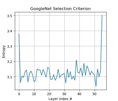
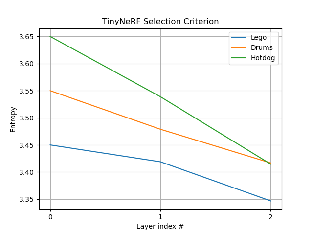
(a)	(b)	(c)
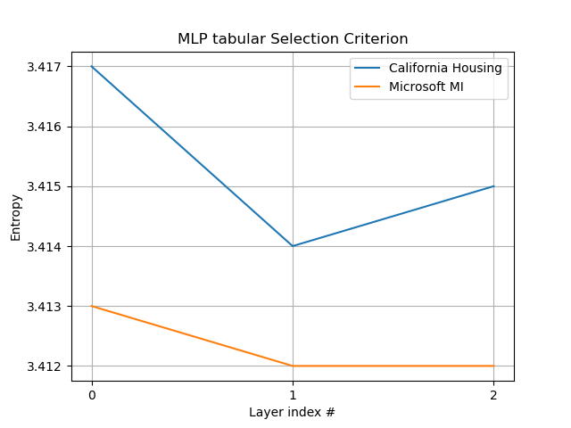
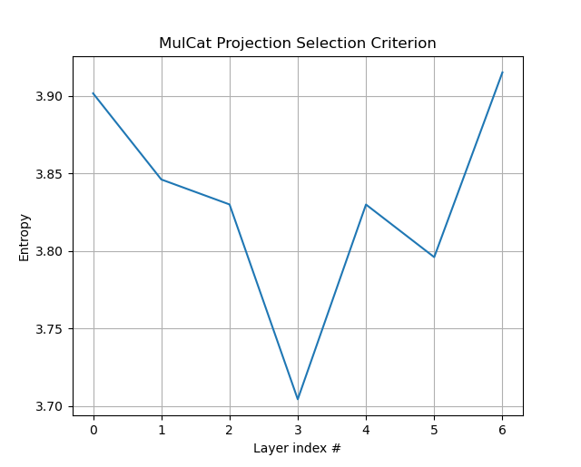
(d)	(e)

Figure 3: Layer Selection Criterion for different experiments. (a) For LeNet5 on MNIST, the next to last Fully-Connected layer is selected since it has the maximal entropy. (b) For GoogleNet on CIFAR10, the last Fully-Connected layer is selected. (c) For TinyNeRF (three datasets), the first Fully-Connected layer is selected. (d) For Tabular MLP the first layer is selected. (e) For MulCat the last projection layer is selected.

Appendix C TinyNeRF sample results

Fig. 4 presents sample results for the reconstruction of the Lego/Hotdog/Drums Model. The quality of the OCD results approaches that of the model that overfits on the test view.

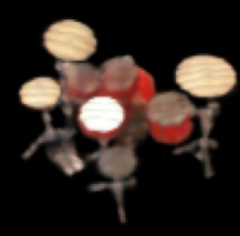
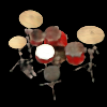
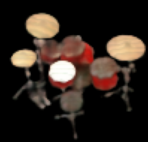
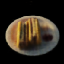
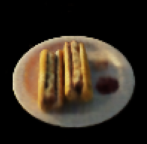
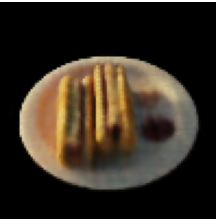
(a)	(b)	(c)

Figure 4: Sample TinyNeRF results on the Drums/Lego/Hotdog model. (a) Base model on a test view. (b) Same test view, overfitted using the ground truth (c) OCD (ours).

Appendix D Cross entropy statistics for the NLP experiments

Table 8 depicts the cross entropy loss for the NLP task of few-shot classification using SetFIT+OCD, when using one random initialization of the diffusion process or when averaging the networks obtained by five random initializations.

Method	SST-5	AmazonCF	CR	Emotion	EnronSpam
One instance	$0.45\pm 0.19$	$0.65\pm 0.30$	$0.41\pm 0.11$	$0.63\pm 0.31$	$0.39\pm 0.20$
Mean network of 5 instances	$0.42\pm 0.20$	$0.61\pm 0.25$	$0.39\pm 0.11$	$0.59\pm 0.32$	$0.38\pm 0.19$

Table 8: The Cross-Entropy loss for the NLP task of few-shot classification with 8 samples per class using SetFIT + OCD, comparing one instance to the mean network obtained with 5 instances.

References

- Alet et al. (2021) Alet, F., Bauza, M., Kawaguchi, K., Kuru, N. G., Lozano-Pérez, T., and Kaelbling, L. Tailoring: encoding inductive biases by optimizing unsupervised objectives at prediction time. Advances in Neural Information Processing Systems, 34:29206–29217, 2021.
- Alpaydin & Jordan (1996) Alpaydin, E. and Jordan, M. I. Local linear perceptrons for classification. IEEE Transactions on Neural Networks, 7(3):788–794, 1996.
- Amit et al. (2021) Amit, T., Nachmani, E., Shaharbany, T., and Wolf, L. Segdiff: Image segmentation with diffusion probabilistic models. arXiv preprint arXiv:2112.00390, 2021.
- Bertinetto et al. (2016) Bertinetto, L., Henriques, J. F., Valmadre, J., Torr, P., and Vedaldi, A. Learning feed-forward one-shot learners. In Advances in Neural Information Processing Systems, pp. 523–531, 2016.
- Bottou & Vapnik (1992) Bottou, L. and Vapnik, V. Local learning algorithms. Neural Computation, 4(6):888–900, 1992. doi: 10.1162/neco.1992.4.6.888.
- Brock et al. (2018) Brock, A., Lim, T., Ritchie, J., and Weston, N. SMASH: One-shot model architecture search through hypernetworks. In International Conference on Learning Representations, 2018. URL https://openreview.net/forum?id=rydeCEhs-.
- Chen et al. (2020) Chen, N., Zhang, Y., Zen, H., Weiss, R. J., Norouzi, M., and Chan, W. Wavegrad: Estimating gradients for waveform generation. arXiv preprint arXiv:2009.00713, 2020.
- Choi et al. (2021) Choi, J., Kim, S., Jeong, Y., Gwon, Y., and Yoon, S. Ilvr: Conditioning method for denoising diffusion probabilistic models. In 2021 IEEE/CVF International Conference on Computer Vision (ICCV), pp. 14347–14356. IEEE, 2021.
- Dhariwal & Nichol (2021a) Dhariwal, P. and Nichol, A. Diffusion models beat gans on image synthesis. Advances in Neural Information Processing Systems, 34:8780–8794, 2021a.
- Dhariwal & Nichol (2021b) Dhariwal, P. and Nichol, A. Diffusion models beat gans on image synthesis. Advances in Neural Information Processing Systems, 34:8780–8794, 2021b.
- Dovrat et al. (2021) Dovrat, S., Nachmani, E., and Wolf, L. Many-speakers single channel speech separation with optimal permutation training. In INTERSPEECH, 2021.
- Gorishniy et al. (2021) Gorishniy, Y., Rubachev, I., Khrulkov, V., and Babenko, A. Revisiting deep learning models for tabular data. Advances in Neural Information Processing Systems, 34:18932–18943, 2021.
- Ha et al. (2016) Ha, D., Dai, A., and Le, Q. V. Hypernetworks. arXiv preprint arXiv:1609.09106, 2016.
- Han et al. (2021) Han, X., Zhang, Z., Ding, N., Gu, Y., Liu, X., Huo, Y., Qiu, J., Yao, Y., Zhang, A., Zhang, L., et al. Pre-trained models: Past, present and future. AI Open, 2:225–250, 2021.
- Ho et al. (2020) Ho, J., Jain, A., and Abbeel, P. Denoising diffusion probabilistic models. Advances in Neural Information Processing Systems, 33:6840–6851, 2020.
- Ho et al. (2022) Ho, J., Saharia, C., Chan, W., Fleet, D. J., Norouzi, M., and Salimans, T. Cascaded diffusion models for high fidelity image generation. Journal of Machine Learning Research, 23(47):1–33, 2022.
- Huang & Belongie (2017) Huang, X. and Belongie, S. Arbitrary style transfer in real-time with adaptive instance normalization. In Proceedings of the IEEE international conference on computer vision, pp. 1501–1510, 2017.
- Jayakumar et al. (2020) Jayakumar, S. M. et al. Multiplicative interactions and where to find them. In International Conference on Learning Representations, 2020.
- Kelley Pace & Barry (1997) Kelley Pace, R. and Barry, R. Sparse spatial autoregressions. Statistics Probability Letters, 33(3):291–297, 1997. ISSN 0167-7152. doi: https://doi.org/10.1016/S0167-7152(96)00140-X. URL https://www.sciencedirect.com/science/article/pii/S016771529600140X.
- Kingma & Ba (2014) Kingma, D. P. and Ba, J. Adam: A method for stochastic optimization. arXiv preprint arXiv:1412.6980, 2014.
- Klein et al. (2015) Klein, B., Wolf, L., and Afek, Y. A dynamic convolutional layer for short range weather prediction. In Proc. IEEE Conference on Computer Vision and Pattern Recognition, pp. 4840–4848, 2015.
- Kong et al. (2021) Kong, Z., Ping, W., Huang, J., Zhao, K., and Catanzaro, B. Diffwave: A versatile diffusion model for audio synthesis. In International Conference on Learning Representations, 2021.
- Krizhevsky et al. (2009) Krizhevsky, A., Hinton, G., et al. Learning multiple layers of features from tiny images. 2009.
- Le & Yang (2015) Le, Y. and Yang, X. Tiny imagenet visual recognition challenge. CS 231N, 7(7):3, 2015.
- LeCun & Cortes (2010) LeCun, Y. and Cortes, C. MNIST handwritten digit database. http://yann.lecun.com/exdb/mnist/, 2010. URL http://yann.lecun.com/exdb/mnist/.
- Lecun et al. (1998) Lecun, Y., Bottou, L., Bengio, Y., and Haffner, P. Gradient-based learning applied to document recognition. Proceedings of the IEEE, 86(11):2278–2324, 1998. doi: 10.1109/5.726791.
- Levkovitch et al. (2022) Levkovitch, A., Nachmani, E., and Wolf, L. Zero-shot voice conditioning for denoising diffusion tts models. In INTERSPEECH, 2022.
- Liu et al. (2022) Liu, H., Tam, D., Muqeeth, M., Mohta, J., Huang, T., Bansal, M., and Raffel, C. Few-shot parameter-efficient fine-tuning is better and cheaper than in-context learning. arXiv preprint arXiv:2205.05638, 2022.
- Liu et al. (2021a) Liu, J., Li, C., Ren, Y., Chen, F., Liu, P., and Zhao, Z. Diffsinger: Singing voice synthesis via shallow diffusion mechanism. arXiv preprint arXiv:2105.02446, 2021a.
- Liu et al. (2021b) Liu, Z., Lin, Y., Cao, Y., Hu, H., Wei, Y., Zhang, Z., Lin, S., and Guo, B. Swin transformer: Hierarchical vision transformer using shifted windows. In Proceedings of the IEEE/CVF International Conference on Computer Vision, pp. 10012–10022, 2021b.
- Lorraine & Duvenaud (2018) Lorraine, J. and Duvenaud, D. Stochastic hyperparameter optimization through hypernetworks. arXiv preprint arXiv:1802.09419, 2018.
- Luhman & Luhman (2021) Luhman, E. and Luhman, T. Knowledge distillation in iterative generative models for improved sampling speed. arXiv preprint arXiv:2101.02388, 2021.
- Lutati & Wolf (2021) Lutati, S. and Wolf, L. Hyperhypernetwork for the design of antenna arrays. In International Conference on Machine Learning, pp. 7214–7223. PMLR, 2021.
- Lutati et al. (2022) Lutati, S., Nachmani, E., and Wolf, L. Sepit: Approaching a single channel speech separation bound. In INTERSPEECH, 2022.
- Mildenhall et al. (2021) Mildenhall, B., Srinivasan, P. P., Tancik, M., Barron, J. T., Ramamoorthi, R., and Ng, R. Nerf: Representing scenes as neural radiance fields for view synthesis. Communications of the ACM, 65(1):99–106, 2021.
- Mitchell et al. (2021) Mitchell, E., Lin, C., Bosselut, A., Finn, C., and Manning, C. D. Fast model editing at scale. In International Conference on Learning Representations, 2021.
- Murthy (2020) Murthy, K. nerf-pytorch. https://github.com/krrish94/nerf-pytorch/blob/master/tiny_nerf.py, 2020.
- Nachmani et al. (2020) Nachmani, E., Adi, Y., and Wolf, L. Voice separation with an unknown number of multiple speakers. In International Conference on Machine Learning, pp. 7164–7175. PMLR, 2020.
- Popov et al. (2020) Popov, S., Morozov, S., and Babenko, A. Neural oblivious decision ensembles for deep learning on tabular data. In International Conference on Learning Representations, 2020. URL https://openreview.net/forum?id=r1eiu2VtwH.
- Popov et al. (2021) Popov, V., Vovk, I., Gogoryan, V., Sadekova, T., and Kudinov, M. Grad-tts: A diffusion probabilistic model for text-to-speech. In International Conference on Machine Learning, pp. 8599–8608. PMLR, 2021.
- Qin & Liu (2013) Qin, T. and Liu, T.-Y. Introducing letor 4.0 datasets. arXiv preprint arXiv:1306.2597, 2013.
- Riegler et al. (2015) Riegler, G., Schulter, S., Ruther, M., and Bischof, H. Conditioned regression models for non-blind single image super-resolution. In Proceedings of the IEEE International Conference on Computer Vision, pp. 522–530, 2015.
- Ronneberger et al. (2015) Ronneberger, O., Fischer, P., and Brox, T. U-net: Convolutional networks for biomedical image segmentation. In International Conference on Medical image computing and computer-assisted intervention, pp. 234–241. Springer, 2015.
- Saharia et al. (2022) Saharia, C., Chan, W., Saxena, S., Li, L., Whang, J., Denton, E., Ghasemipour, S. K. S., Ayan, B. K., Mahdavi, S. S., Lopes, R. G., et al. Photorealistic text-to-image diffusion models with deep language understanding. arXiv preprint arXiv:2205.11487, 2022.
- San-Roman et al. (2021) San-Roman, R., Nachmani, E., and Wolf, L. Noise estimation for generative diffusion models. arXiv preprint arXiv:2104.02600, 2021.
- Shamsian et al. (2021) Shamsian, A., Navon, A., Fetaya, E., and Chechik, G. Personalized federated learning using hypernetworks. In International Conference on Machine Learning, pp. 9489–9502. PMLR, 2021.
- Silverman (1986) Silverman, B. W. Density Estimation for Statistics and Data Analysis. Chapman & Hall, London, 1986.
- Simonyan & Zisserman (2014) Simonyan, K. and Zisserman, A. Very deep convolutional networks for large-scale image recognition. arXiv preprint arXiv:1409.1556, 2014.
- Sohl-Dickstein et al. (2015) Sohl-Dickstein, J., Weiss, E., Maheswaranathan, N., and Ganguli, S. Deep unsupervised learning using nonequilibrium thermodynamics. In International Conference on Machine Learning, pp. 2256–2265. PMLR, 2015.
- Song et al. (2020) Song, J., Meng, C., and Ermon, S. Denoising diffusion implicit models. In International Conference on Learning Representations, 2020.
- Szegedy et al. (2015) Szegedy, C., Liu, W., Jia, Y., Sermanet, P., Reed, S., Anguelov, D., Erhan, D., Vanhoucke, V., and Rabinovich, A. Going deeper with convolutions. In Proceedings of the IEEE conference on computer vision and pattern recognition, pp. 1–9, 2015.
- Touvron et al. (2022) Touvron, H., Cord, M., and Jégou, H. Deit iii: Revenge of the vit. arXiv preprint arXiv:2204.07118, 2022.
- Tunstall et al. (2022) Tunstall, L., Reimers, N., Jo, U. E. S., Bates, L., Korat, D., Wasserblat, M., and Pereg, O. Efficient few-shot learning without prompts. arXiv preprint arXiv:2209.11055, 2022.
- Vaswani et al. (2017) Vaswani, A., Shazeer, N., Parmar, N., Uszkoreit, J., Jones, L., Gomez, A. N., Kaiser, Ł., and Polosukhin, I. Attention is all you need. Advances in neural information processing systems, 30, 2017.
- von Oswald et al. (2020) von Oswald, J., Henning, C., Sacramento, J., and Grewe, B. F. Continual learning with hypernetworks. In International Conference on Learning Representations, 2020.
- Wang et al. (2021) Wang, D., Shelhamer, E., Liu, S., Olshausen, B., and Darrell, T. Tent: Fully test-time adaptation by entropy minimization. In International Conference on Learning Representations, 2021. URL https://openreview.net/forum?id=uXl3bZLkr3c.
- Watson et al. (2021) Watson, D., Ho, J., Norouzi, M., and Chan, W. Learning to efficiently sample from diffusion probabilistic models. arXiv preprint arXiv:2106.03802, 2021.
- Wolf et al. (2009) Wolf, L., Hassner, T., and Taigman, Y. The one-shot similarity kernel. In 2009 IEEE 12th International Conference on Computer Vision, pp. 897–902. IEEE, 2009.
- Zhang et al. (2019) Zhang, C., Ren, M., and Urtasun, R. Graph hypernetworks for neural architecture search. In Int. Conf. on Learning Representations, 2019. URL https://openreview.net/forum?id=rkgW0oA9FX.
- Zhang et al. (2006) Zhang, H., Berg, A. C., Maire, M., and Malik, J. Svm-knn: Discriminative nearest neighbor classification for visual category recognition. In CVPR, volume 2, pp. 2126–2136. IEEE, 2006.