Speed Up the Cold-Start Learning in Two-Sided Bandits with Many Arms

Speed Up the Cold-Start Learning in Two-Sided Bandits with Many Arms

Mohsen Bayati Graduate School of Business, Stanford University, bayati@stanford.edu Junyu Cao McCombs School of Business, The University of Texas at Austin, junyu.cao@mccombs.utexas.edu Wanning Chen Foster School of Business, University of Washington, wnchen@uw.edu

Multi-armed bandit (MAB) algorithms are efficient approaches to reduce the opportunity cost of online experimentation and are used by companies to find the best product from periodically refreshed product catalogs. However, these algorithms face the so-called cold-start at the onset of the experiment due to a lack of knowledge of customer preferences for new products, requiring an initial data collection phase known as the burn-in period. During this period, MAB algorithms operate like randomized experiments, incurring large burn-in costs which scale with the large number of products. We attempt to reduce the burn-in by identifying that many products can be cast into two-sided products, and then naturally model the rewards of the products with a matrix, whose rows and columns represent the two sides respectively. Next, we design two-phase bandit algorithms that first use subsampling and low-rank matrix estimation to obtain a substantially smaller targeted set of products and then apply a UCB procedure on the target products to find the best one. We theoretically show that the proposed algorithms lower costs and expedite the experiment in cases when there is limited experimentation time along with a large product set. Our analysis also reveals three regimes of long, short, and ultra-short horizon experiments, depending on dimensions of the matrix. Empirical evidence from both synthetic data and a real-world dataset on music streaming services validates this superior performance.

online experimentation, multi-armed bandit with many arms, cold-start, low-rank matrix.

1 Introduction

Online experimentation has been a major force in assessing different versions of a product, finding better ways to engage customers and generating more revenue. These experiments happen on a recurring basis with periodically refreshed product catalogs. One family of online experimentation is the so-called multi-armed bandit (MAB) algorithms, where each arm models a version of the product. At each time period, the decision-maker tests out a version, learns from the observed outcome, and proceeds to the next time period. Bandit algorithms can dynamically allocate experimentation effort to versions that are performing well, in the meantime allocating less effort to versions that are underperforming. These algorithms have gained much attention in recent years because they can identify the optimal product quickly under relatively low opportunity cost, which is incurred by selecting suboptimal products. Consequently, they manage to reduce customers’ exposure to a potentially inferior experience. We want to highlight that what is treated as product in this context is not confined to merchandise in the e-commerce setting. It includes broader categories from ads campaign product in online advertisement to drug product in drug development.

At the onset of the experimentation, MAB algorithms face what is known as the cold-start problem when there is a large product set: many versions of a product are brand new to the customers. It is not yet clear to the algorithms how to draw any useful inferences before gathering some information. Therefore, many of MAB algorithms involve an initial data collection phase, known as the burn-in period (Lu 2019). During this period, MAB algorithms operate as nearly equivalent to randomized experiments, incurring costs that scale with the number of products. Under such circumstances, the cumulative cost, or regret, of current practices is huge due to a costly and lengthy burn-in period.

Our goal is to come up with a framework that can be cost-effective, which is achieved by first identifying a two-sided structure of the products. In many of the applications, because the products have two major components, the bandit arms can be viewed as versions of a two-sided product. To be more specific, let us provide two examples that will reappear in the later empirical studies.

Example 1.1

Consider an online platform that wants to select one user segment and one content creator segment that interact the most to target an advertisement campaign. Such advertisement campaign is a two-sided product since user segment and content creator segment are its two sides. There are many user segments and many content creator segments. In each time period, the platform tests a pair of user segment and content creator segment and observes the amount of interaction between them, based on which the platform decides which pair to test next. The number of products scales quickly: ten user segments and ten content creator segments already give rise to one hundred pairs, and this is just an underestimate of how many segments there are for each side.

Example 1.2

Consider an online platform that wants to design a homepage with a headline and an image. The platform’s goal is to select a pair of homepage and headline that attracts the most amount of user engagement. The homepage design is a two-sided product with headline and image as two sides. Similar to Example 1.1, the number of pairs can easily be over several hundreds.

Besides the two examples above, there are plenty of other two-sided products: Airbnb experiences (activities and locations), Stitch Fix personal styling (tops and pants), Expedia travel (hotels and flights), car sales (packages and prices), drug development (composition of ingredients and dosages) and so on.

The task of finding the best version of a two-sided product can be translated into finding the maximum entry of a partially observed reward matrix, which can help accelerate the learning process. That is, we can model different choices of one side to be rows of the matrix, different choices of the other side to be the columns, and the unknown rewards for the corresponding row-column pairs (e.g. the amount of interaction in Example 1.1 and the amount of user engagement in Example 1.2) to be the matrix entries. Mathematically, suppose the first side of the product has $d_{r}$ number of choices and the second side has $d_{c}$ number of choices, then this matrix contains the rewards of $d_{r}d_{c}$ versions of the two-sided product as entries. As aforementioned, current algorithms will randomize on the initial $\Omega(d_{r}d_{c})$ number of periods, leading to a very costly burn-in period as $d_{r}$ and $d_{c}$ are often very large. Furthermore, when the time horizon $T$ is rather small compared to the order $d_{r}d_{c}$, a large cumulative regret that scales with $d_{r}d_{c}$ would ensue. By casting the rewards into a matrix and considering its low-dimensional approximation, we can reduce the regret by orders of magnitudes.

Specifically, it is the natural low-rank structure of the underlying ground truth reward matrix that helps expedite the experiment. Intuitively, the rewards for different versions of a two-sided product depend on the interactions between some latent features of the two sides. Low-rank simply means that we only need as few as $\mathfrak{r}$ latent features to explain each side, such that $\mathfrak{r}\ll\min(d_{r},d_{c})$, where $\mathfrak{r}$ is the rank of the matrix. Because of such low-rank property and with the help from low-rank matrix estimators, we only need to collect very few data to have an estimate of the rewards for all arms of interest in the burn-in period that is accurate enough to help screen out majority of the sub-optimal arms, and hence requiring substantially less downstream exploration which greatly reduces the burn-in cost.

1.1 Our Contributions

Algorithm. Specifically, we have designed a new and efficient bandit algorithm called the Low-Rank Bandit. The algorithm and its variation via submatrix sampling can efficiently choose from a large product set of two-sided products given a short time horizon. It is split into two phases: “pure exploration phases” and “targeted exploration + exploitation phases”. At each period, the algorithm follows a schedule to enter either of the two phases. If it is in a pure exploration phase, a forced sample is selected uniformly at random and is used for the low-rank matrix estimation. The forced-sample estimates are used to screen out arms that are far from the optimal arm. The remaining arms form a targeted set whose size is much smaller than the initial product set. If the algorithm is in a targeted exploration + exploitation phase, we choose a product based on an off-the-shelf stochastic multi-armed bandit algorithm (e.g. UCB, Thompson Sampling) applied on the current targeted set. For illustration purpose, we will use UCB algorithm throughout the paper.

We introduce a subsampling technique when we are extremely sensitive about time. Given an ultra-short horizon (formally defined in Section 3.6) in the face of a huge number of arms, we can instead sample a submatrix of smaller dimensions and apply the Low-Rank Bandit to it. The intuition behind this is as follows. Even though the best entry in the submatrix might be suboptimal, because the horizon is ultra-short, the cost we save from not exploring the much larger matrix compensates for the regret we incur from picking a suboptimal entry.

Theory. We establish non-asymptotic dependent and independent regret bounds and show that the Low-Rank Bandit achieves expected cumulative regret that scales with $d_{r}+d_{c}$ rather than $d_{r}d_{c}$. Most existing theoretical analysis for bandit algorithms study dependence of the regret on the time horizon asymptotically and may not perform well when the time horizon is short. Unlike them, ours shed light on customized strategies given different time horizon lengths and the product set sizes.

A crucial step in our regret analysis is providing entry-wise estimation error bound. However, most existing matrix estimation results provide a bound on the estimation error of the entire matrix, which would be a crude upper bound for our task. Rather, using estimation error on each row to bound entry-wise estimation error, realized by the “row-enhancement” procedure (Hamidi et al. 2019), saves us an unnecessary $\sqrt{\max(d_{r},d_{c})}$ factor.

Empirics. Empirical evidence from both synthetic data and a real-world dataset on music streaming services validates the superior performance of our algorithm. Numerical simulations demonstrate that the Low-Rank Bandit significantly outperforms benchmarks in the cumulative regret, under various time horizon lengths. With the real data, we apply the Low-Rank Bandit to learn the best combination of user group and creator group to target for an advertisement campaign. We show that our algorithm significantly outperforms existing bandit algorithms in finding the best combination efficiently. In particular, the Low-Rank Bandit (via its submatrix sampling version) successfully leverages limited amount of available data to make better decisions in ultra-short horizon, while continuing to perform well in longer horizon regimes.

A reduction model for contextual bandits. We propose a new modeling framework to transform a stochastic linear bandit setting (a general class of bandit problems that contains contextual bandits) to the scope of our low-rank bandit problem. This allows us to empirically showcase the Low-Rank Bandit’s effectiveness of reducing the burn-in in contextual settings by comparing it with a canonical linear bandit method, OFUL.

1.2 Related Literature

We will first give an overview of the bandit literature since our work addresses the setting of online decision making under bandit feedback. Next, because our work evolves around low-rank models and matrix-shaped data, we will introduce relevant literature to those topics as well.

The bandit problem originates from the field of online experimentation. There are different objectives, including regret minimization and best-arm identification (Gabillon et al. 2012, Russo 2016). Our work focuses on the former objective, where algorithms such as Thompson Sampling (Thompson 1933, Agrawal and Goyal 2012, Gopalan et al. 2014, Russo et al. 2017) and Upper Confidence Bound (Lai 1987, Katehakis and Robbins 1995, Kaelbling 1993, Auer et al. 2002a) are some canonical works for i.i.d. stochastic bandits. Like ours, these algorithms explore and exploit without contextual information. That is, they make no assumptions on dependence of the arm rewards. There is also a large literature on bandit problems with contextual information, when the arm rewards are parametric function of the observed contexts. Linear bandit (Auer et al. 2002b, Dani et al. 2008, Rusmevichientong and Tsitsiklis 2010, Li et al. 2010, Chu et al. 2011, Agrawal and Devanur 2014, Abbasi-Yadkori et al. 2011) and its extension under generalized linear models (GLM) (Filippi et al. 2010, Li et al. 2017, Kveton et al. 2020) have been under the spotlight of many works. As the name of linear bandit suggests, the arm rewards are linear functions of the observed contexts. We refer the readers to Lattimore and Szepesvári (2020) for more information on bandit algorithms.

However, as discussed earlier, existing bandit algorithms perform very poorly when there are many arms due to the linear dependence of the cumulative regret on the number of arms at the beginning of the experiment. Such a cold-start problem is commonly seen in online experimentation and there is a substantial amount of literature on this topic (Ye et al. 2020, Lika et al. 2014, Zhang et al. 2014, Volkovs et al. 2017). Examples of existing works to overcome the cold-start problem involve combining clustering and MAB algorithms (Miao et al. 2019, Keskin et al. 2020), warm starting the bandit problem using historical data (Banerjee et al. 2022), or using an integer program to constrain the action set Bastani et al. (2022). A separate stream of literature studying many-armed or infinitely-armed bandit problems has addressed this cold-start problem by using subsampling to reduce the opportunity cost (Berry et al. 1997, Bonald and Proutiere 2013, Wang et al. 2009, Audibert et al. 2007, Carpentier and Valko 2015, Chaudhuri and Kalyanakrishnan 2018, Bayati et al. 2020). The main differentiating factor between our work and this literature is that the inherent matrix structure of the two-sided products allows us to make a more informed selection of the arms to use for targeted exploration + exploitation.

An alternative solution to tackle infinitely-armed bandit problems is to assume that the reward function is a linear function of actions that belong to a compact set, e.g., as in (Mersereau et al. 2009, Rusmevichientong and Tsitsiklis 2010). In such cases, pulling any action provides information for reward function of all actions. However, in our two-sided products setting such information sharing is only available if two arms are in the same row or in the same column of the matrix of products.

Low-rank matrix structure has joined force with bandit settings in many other works (Katariya et al. 2017, Trinh et al. 2020, Kveton et al. 2017). They considered different set-ups than ours.

Jun et al. (2019) incorporated low-rank matrix structure as well in their algorithm, addressing the contextual setting.

Lu et al. (2020) proposed a UCB-type algorithm for low-rank generalized linear models. The ESTR algorithm in Jun et al. (2019) and LowESTR algorithm in Lu et al. (2020) use a novel way of exploiting the subspace so as to reduce the problem to linear bandits after exploration. However, both methods are not efficiently implementable because of the exponentially weighted average forecaster for solving the online low-rank linear prediction problem. Kallus and Udell (2020) imposed a low-rank structure to their underlying parameter matrix. However, they analyzed the dynamic assortment personalization problem in which a decision maker picks a best subset of products for a user, with quite different settings and models from ours.

Hamidi et al. (2019) also imposed a low-rank structure on the arm parameter set to expedite the learning process, but in their setting, contexts are observed which is different from ours. Nakamura (2015) proposed a heuristic UCB-like strategy of collaborative filtering for a recommendation problem that selects the best user-item pairs, which they called the direct mail problem, but no theoretical guarantee for that approach is known. Sam et al. (2022) studied a class of Markov decision processes that exhibits latent low-dimensional structure with respect to the relationship between large number of states and actions. Zhu et al. (2022) considered learning the Markov transition matrix under the low-rank structure. For other low-rank bandit works, we refer the readers to Lu et al. (2018) and Hao et al. (2020).

Though the low-rank structure is utilized in all the above-mentioned works, we want to emphasize that our work focuses on a short-horizon many arms learning problem, and the purpose of utilizing the low-rank property is to efficiently filter suboptimal arms in order to construct a more focused targeted set, under very limited experimentation time.

Low-rank matrix estimators are building blocks for many applications that have inherent low-rank models (Athey et al. 2021, Farias et al. 2021, Agarwal et al. 2021). For a survey paper on low-rank matrix estimators, we refer the readers to Davenport and Romberg (2016) and Chen et al. (2020) for a detailed discussion.

There are recent papers such as (Gupta and Rusmevichientong 2021, Gupta and Kallus 2022) and (Allouah et al. 2021, Besbes and Mouchtaki 2021) that focused on practical small data regime with limited sample size: the former group studied how to optimize decison-making in a large number of small-data problems, while the latter group studied classical pricing and newsvendor problems and showed how a small number of samples can provide valuable information, leveraging structure of the problems. Even though we focus on the burn-in period with small data, our bandit formulation with two-sided products and low-rank structure is completely different from their offline set-ups. Our problem is also different from the recent work of Xu and Bastani (2021) that studied how one can learn across many contextual bandit problems, because in our model the contexts are hidden and will be estimated through learning of the low-rank structure.

Finally, we note that recent works such as Bajari et al. (2021) and Johari et al. (2022) also looked at online experimentation for two-sided settings. However, they looked at a completely different problem. Specifically, their objective is to remove bias due to the spillover effect by using two-sided randomization.

1.3 Organization of the Paper

The remainder of the paper is organized as follows. We describe the problem formulation in Section 2. We present the Low-Rank Bandit algorithm and our main result on the algorithm’s performance in Section 3. In Section 4, we present the Submatrix Sampling technique to further enhance Low-Rank Bandit’s performance when the time horizon is ultra-short. Finally, empirical results on simulated data as well as our evaluation on real music streaming data for the task of advertisement targeting are presented in Section 5. It also includes numerical comparison against linear bandits in contextual settings.

2 Model and Problem

In this section, we formally introduce the learning and decision-making problem that we study. For this, we consider a stochastic multi-armed bandit with (two-sided) arms represented as row-column pairs of a matrix and arm mean rewards represented as entries of the matrix. We explain what it means for the reward matrix to have a low-rank structure, paving our way to understand the Low-Rank Bandit algorithm. We also introduce some necessary notation and assumptions that will be used throughout the paper. We use bold capital letters (e.g. $\operatorname{\mathbf{B}}$) for matrices and non-bold capital letters for vectors (e.g., $V$, except for $T$, which denotes the total time horizon). For a positive integer $m$, we denote the set of integers $\{1,\ldots,m\}$ by $[m]$. For a matrix $\operatorname{\mathbf{B}}$, $\operatorname{\mathbf{B}}_{ij}$ refers to its entry $(i,j)$ and $\operatorname{\mathbf{B}}_{j}$ refers to its $j$-th row.

2.1 Rewards as a Low-Rank Matrix

We work with a $d_{r}\times d_{c}$ matrix $\operatorname{\mathbf{B}}^{*}$ and our goal is to find the entry with the biggest reward as we sequentially observe noisy version of picked entries. As introduced earlier, the $d_{r}$ number of rows of this matrix correspond to $d_{r}$ different choices for the first side of the two-sided products and the $d_{c}$ number of columns correspond to different choices for the second side. Entries of $\operatorname{\mathbf{B}}^{*}$ correspond to the mean rewards for different combinations of the two sides and we assume they are bounded. However, to simplify the mathematical expressions in the analysis, we assume $\ell_{2}$-norm of each row is bounded by $b^{*}$, which absorbs a factor of $\sqrt{d_{c}}$. [Boundedness] Assume $\|\operatorname{\mathbf{B}}^{*}\|_{\infty,2}\leq b^{*}$, where $\|\cdot\|_{\infty,2}$ denotes the largest $\ell_{2}$-norm among the rows of a matrix, i.e.,

$$\|\operatorname{\mathbf{B}}\|_{\infty,2}=\max_{j\in[d_{r}]}\left(\sum_{k=1}^{d_{c}}|\operatorname{\mathbf{B}}_{jk}|^{2}\right)^{1/2}.$$

This is a standard assumption made in the bandit literature, making sure that the maximum regret at any time step is bounded. This is likely satisfied since user preferences are bounded in practice.

We will use the two-sided product in Example 1.1, ads campaign, as a running example. In this case, the marketer needs to pick a pair of user segment and content creator segment to target the ads. Then we can model user segments as rows of matrix $\operatorname{\mathbf{B}}^{*}$ and content creator segments as columns of matrix $\operatorname{\mathbf{B}}^{*}$. The amount of interaction between different combinations of user segments and content creator segments are the entries of $\operatorname{\mathbf{B}}^{*}$. The goal under this scenario is to find the pair that interacts the most to target the ads by experimenting with different pairs.

We model the ground truth mean reward matrix as a low-rank matrix. That is, let $\mathfrak{r}$ be the rank of $\operatorname{\mathbf{B}}^{*}$, we have $\mathfrak{r}\ll\min\{d_{r},d_{c}\}$. This means the reward for the entry corresponding to row $j$ and column $k$ is a dot product of two $\mathfrak{r}$-dimensional latent feature vectors. Therefore, our reward model is a contextual reward with unobserved features. In Section 5.3 we show an alternative contextual bandit representation of our reward function that is motivated by the standard linear bandit setting framework.

Motivated by the literature on low-rank matrix completion, we introduce the row-incoherence parameter that is related to the rank of the matrix. It quantifies how much information observing an entry gives about other entries in a matrix.

Definition 2.1

For a $d_{r}\times d_{c}$ matrix $\operatorname{\mathbf{B}}$ of rank $\mathfrak{r}$ with singular value decomposition $\operatorname{\mathbf{B}}=\operatorname{\mathbf{U}}\operatorname{\mathbf{D}}\operatorname{\mathbf{V}}^{\top}$, we define the row-incoherence parameter as

$$\mu(\operatorname{\mathbf{B}})=\sqrt{\frac{d_{r}}{\mathfrak{r}}}\cdot\frac{\|\operatorname{\mathbf{B}}\|_{\infty,2}}{\operatorname{\mathbf{D}}_{\mathfrak{r}\mathfrak{r}}}\,.$$ (2.1)

We let $\mu^{*}:=\mu(\operatorname{\mathbf{B}}^{*})$ denote the row-incoherence parameter for the ground truth matrix $\operatorname{\mathbf{B}}^{*}$. Intuitively, the more information about other products we can get from observing an entry, the more tractable it is to estimate the rewards for all products based on a limited number of observed entries. Such a reward matrix is more incoherent. Consequently, less experimentation cost is incurred to explore among a large product set. In contrast, coherent matrices are those which have most of their mass in a relatively small number of elements and are much harder to recover under limited observations. They tend to have larger row-incoherence parameters. The notion of incoherence was introduced by Candes and Recht (2009) and Keshavan et al. (2010) and has been widely adopted in the matrix-completion literature.

2.2 Bandit under the Matrix-Shaped Rewards

Consider a $T$-period horizon for the experimentation; at each time step $t$, the marketer has access to $d_{r}d_{c}$ arms (ads campaigns) and each arm yields an uncertain reward (amount of interaction). At time $t$, if the marketer pulls arm $(j_{t},k_{t})\in[d_{r}]\times[d_{c}]$, it yields reward

$$y_{t}:=\operatorname{\mathbf{B}}^{*}_{j_{t}k_{t}}+\epsilon_{t}\,,$$

where we assume the observational noises $\epsilon_{t}$ to be independent 1-subgaussian random variables.

Natural examples of subgaussian random variables include any centered and bounded random variable, or a centered Gaussian.

Our task is to design a sequential decision-making policy $\pi$ that learns the underlying arm rewards (parameter matrix $\operatorname{\mathbf{B}}^{*}$) over time in order to maximize the expected reward. Let $\pi_{t}=(j_{t},k_{t})$, an element of $[d_{r}]\times[d_{c}]$, denote the arm chosen by policy $\pi$ at time $t\in[T]$. We compare to an oracle policy $\pi^{*}$ that already knows $\operatorname{\mathbf{B}}^{*}$ and thus always chooses the best arm (in expectation), $\pi^{*}=(j^{*},k^{*})=\argmax_{(j,k)\in[d_{r}]\times[d_{c}]}\operatorname{\mathbf{B}}^{*}_{jk}$. Thus, if the arm $\pi_{t}=(j_{t},k_{t})$ is chosen at time $t$, expected regret incurred is $\mathbb{E}[\operatorname{\mathbf{B}}^{*}_{j^{*}k^{*}}-\operatorname{\mathbf{B}}^{*}_{j_{t}k_{t}}],$ where the expectation is with respect to the randomness of $\epsilon_{t}$ and potential randomness introduced by the policy $\pi$. This is simply the difference in expected rewards of $\pi_{t}^{*}$ and $\pi_{t}$. We seek a policy $\pi$ that minimizes the cumulative expected regret

$$\textnormal{{Regret}}_{\pi}(T)=\sum_{t=1}^{T}\mathbb{E}_{\pi}\left[\operatorname{\mathbf{B}}^{*}_{j^{*}k^{*}}-\operatorname{\mathbf{B}}^{*}_{j_{t}k_{t}}\right]\,.$$

Note that throughout this paper we assume the matrix $\operatorname{\mathbf{B}}^{*}$ is deterministic which means our notion of regret is frequentist.

Together with policy $\pi$, the observation model can be characterized by a trace regression model (Hastie et al. 2015). For a given subset $\mathcal{I}=\{t_{1},\dots,t_{n}\}$ of $[T]$, we define

$$Y=\mathfrak{X}^{\pi}_{\mathcal{I}}(\operatorname{\mathbf{B}}^{*})+E\,,$$

with observation operator $\mathfrak{X}^{\pi}_{\mathcal{I}}$ (defined below), vector of observed values $Y\in\mathbb{R}^{n}$ equal to $[y_{t_{1}},y_{t_{2}},\dots,y_{t_{n}}]^{\top}$, and noise vector $E\in\mathbb{R}^{n}$ equal to $[\epsilon_{t_{1}},\epsilon_{t_{2}},\dots,\epsilon_{t_{n}}]^{\top}$. The observation operator $\mathfrak{X}^{\pi}_{\mathcal{I}}(\cdot)$ takes in a matrix $\operatorname{\mathbf{B}}$ and outputs a vector of dimension $n$ (i.e., $\mathfrak{X}^{\pi}_{\mathcal{I}}:\mathbb{R}^{d_{r}\times d_{c}}\rightarrow\mathbb{R}^{n}$). Elements of the output vector are the entries of $\operatorname{\mathbf{B}}$ at $n$ observed locations, determined by $\pi_{t_{1}},\dots,\pi_{t_{n}}$. Specifically, $\mathfrak{X}^{\pi}_{\mathcal{I}}(\operatorname{\mathbf{B}})$ is a vector in $\mathbb{R}^{n}$, and for each $i$ in $[T]$, its $i$-th entry is defined by

$$\left[\mathfrak{X}^{\pi}_{\mathcal{I}}(\operatorname{\mathbf{B}})\right]_{i}:=\langle\operatorname{\mathbf{B}},\operatorname{\mathbf{X}}_{t_{i}}^{\pi}\rangle\,,$$ (2.2)

where design matrix $\operatorname{\mathbf{X}}_{t_{i}}^{\pi}\in\mathbb{R}^{d_{r}\times d_{c}}$ has all of its entries equal to $0$, except for the $\pi_{t_{i}}=(j_{t_{i}},k_{t_{i}})$-th entry, which is equal to $1$. The notation $\langle\cdot,\cdot\rangle$ refers to the trace inner product of two matrices that is defined by

$$\langle\operatorname{\mathbf{B}}_{1},\operatorname{\mathbf{B}}_{2}\rangle:=\operatorname{Tr}(\operatorname{\mathbf{B}}_{1}\operatorname{\mathbf{B}}_{2}^{\top})\,.$$

The observation operator will appear in the matrix estimator we use.

3 Low-Rank Bandit Algorithm

Intuitively, Low-Rank Bandit algorithm benefits from the low-rank reward structure because such structure allows the algorithm to have a decent understanding of all the arms of interest by only observing a few arms. Thus, we can speed up the cold-start given a relatively short horizon in the face of many arms. In a typical but unrealistic formulation of this problem, the set of arms is assumed to be “small” relative to the time horizon $T$. In particular, in standard asymptotic analysis of the MAB setting, the horizon $T$ scales to infinity while the number of arms remains constant. However, as discussed earlier, the number of arms could be large relative to the time horizon of interest in many practical situations. In such a short horizon, standard MAB algorithms will incur at least $\Omega(d_{r}d_{c})$ regret. By taking advantage of the low-rank matrix structure of the arms, we can shrink the regret to $O(\mathfrak{r}(d_{r}+d_{c}))$.

As mentioned in Section 1.1, Low-Rank Bandit algorithm is constructed using a two-phase approach—it is split into “pure exploration phases” and “targeted exploration + exploitation phases”. This approach partially builds on the ideas in Goldenshluger and Zeevi (2013) that were later extended by Bastani and Bayati (2020), Hamidi et al. (2019). Specifically, those studies centered around the contextual bandit problem. They built two sets of estimators (namely, forced-sample and all-sample estimators) in such a way that the former estimator is used to construct a targeted set that filters sub-optimal arms which fall outside the confidence region of the optimal reward, and the latter estimator is used to select the best arm in the targeted set. The first step which is a pure exploration procedure aims at ensuring that during a constant proportion of time periods, only a single arm is left in the targeted set so the algorithm can collect i.i.d. samples in the second phase, despite the fact that the second phase is pure exploitation.

However, in our study, the two-phase procedure serves a different purpose. More specifically, in the first phase, we utilize the low-rank structure to filter sub-optimal arms that are $\frac{h}{2}$-away from the highest estimated reward by forced-sample estimators, where $h$ is called the filtering resolution and will be discussed in depth in Section 3.3 and Section 3.5. While our first step seems similar to the aforementioned papers, our second phase is itself a UCB algorithm that both explores and exploits the targeted set to find the optimal arm. This distinction results in a different requirement for the first phase: the filtered set does not need to contain just one element; rather, it only needs to be much smaller than $d_{r}\times d_{c}$ to meaningfully reduce the exploration cost of a regular UCB algorithm. This fact results in a different selection criteria for the filtering resolution $h$. As we will discuss in detail later, the optimal value of $h$ is determined by both the matrix size and the total time horizon.

Furthermore, we want to emphasize that the two-phase approach in the aforementioned studies cannot be directly applied to our problem. They focused on long enough experimentation time horizon so that their algorithms can take time to learn arms well and leave only the optimal choice in the targeted set for some fixed $h$. However, as we mentioned before, we are facing a short horizon under many circumstances. Thus it is impossible to construct a targeted set with fine-enough filtering resolution that only contains the optimal choice as the single arm, because forced-sample estimation is not accurate enough under limited experimentation time to achieve that. Indeed, the finer $h$ is, the more accurate forced-sample estimation needs to be. Such will be explained in more details in Lemma 3.4.

Finally, we note that one cannot use the low-rank estimator to construct confidence sets for the UCB algorithm because existing bounds for the low-rank estimators do not work in presence of adaptively collected data. The only exception (to the best of our knowledge) is the all-sampling estimator of Hamidi et al. (2019), but as discussed above, their approach would not work when the targeted set has more than one arm.

3.1 Description of the Algorithm

The main idea of the two-phase algorithm is to reduce the initially large set of arms via a low-rank estimator and pass the smaller set of arms to a UCB algorithm. Specifically, we forced-sample arms at prescribed times and use a sharp low-rank estimator with a row-enhancement procedure to obtain an estimation of each row of $\operatorname{\mathbf{B}}^{*}$ and use that to select a targeted set of arms that with high probability contains the optimal arm.

The Low-Rank Bandit takes as input the matrix row and column dimension $d_{r}$ and $d_{c}$, the forced-sampling rule $f_{\cdot}$, and a filtering resolution $h>0$ (discussed further in Section 3.3). The complete procedure is in Algorithm 1.

Forced-sampling rule:

Our forced-sampling rule is $f:\mathbb{N}^{+}\rightarrow([d_{r}]\times[d_{c}])\cup\{\emptyset\}$. At time $t$, the forced-sampling rule decides between forcing the arm $f_{t}\in[d_{r}]\times[d_{c}]$ to be pulled or exploiting the past data, indicated by $f_{t}=\emptyset$. By $\mathcal{F}_{t}$, we denote the time periods that an arm is forced to be pulled, i.e. $\mathcal{F}_{t}:=\{t^{\prime}\leq t:f_{t^{\prime}}\in[d_{r}]\times[d_{c}]\}$. The forced-sampling rule that we use is a randomized function that picks an arm $(j,k)\in[d_{r}]\times[d_{c}]$ with probability

$$\mathbb{P}\big{(}f_{t}=(j,k)\big{)}=\begin{cases}\frac{1}{d_{r}d_{c}}&\text{ if }t\leq 2\rho\log(\rho),\\ \frac{\rho}{d_{r}d_{c}[t-\rho\log(\rho)+1]}&\text{ if }t>2\rho\log(\rho),\end{cases}$$ (3.1)

and $f_{t}=\emptyset$ otherwise. We will specify the parameter $\rho$ in Section 3.4.

Estimators:

At any time $t$, the Low-Rank Bandit maintains two sets of parameter estimates for $\operatorname{\mathbf{B}}^{*}$:

1. the forced-sample estimates $\widehat{\operatorname{\mathbf{B}}}^{F}$ based only on forced samples. Note that this is obtained by applying a low-rank estimator $\bar{\operatorname{\mathbf{B}}}$ (described in Section 3.2) to the forced samples followed by the row-enhancement procedure (described in Appendix 7);

2. the UCB estimator $\widehat{\operatorname{\mathbf{B}}}^{UCB}_{jk}$ based on all samples observed for each arm $(j,k)$.

Execution:

If the current time $t$ is in $\mathcal{F}_{t}$, then arm $f_{t}$ is played. Otherwise, we follow a two-phase process: first, we use the forced-sample estimates to find the highest estimated reward achievable across all $d_{r}\times d_{c}$ entries. We then select the subset of arms $\mathcal{C}\subset[d_{r}]\times[d_{c}]$ whose estimated rewards are within $h/2$ of the maximum achievable (in step 6 of Algorithm 1). After this pre-processing step, we use the empirical mean estimates to choose the arm with the highest estimated optimistic reward within the set $\mathcal{C}$ (in step 7 of Algorithm 1). The function $w(t)$ used in this step is defined by $w(t)=1+t\log^{2}(t)$ for the empirical experiment and $w(t)=t$ for the analysis part for simpilcity. We will specify how to choose $\lambda$ in the next subsection.

Algorithm 1 Low-Rank Bandit

1:Input: Forced-sampling rule $f$, gap $h$, row dimension $d_{r}$, column dimension $d_{c}$.

2:for $t=1,2,\dots$ do

3:     if $f_{t}\neq\emptyset$ then “pure exploration phase”

4:         $\pi_{t}\leftarrow f_{t}$ (forced-sampling)

5:     else“targeted exploration + exploitation phases”

6:         Define the set of near-optimal arms, $\mathcal{C}$, according to the forced-sample estimator:

$$\mathcal{C}=\Bigg{\{}(j,k)\in[d_{r}]\times[d_{c}]\mid\widehat{\operatorname{\mathbf{B}}}_{jk}^{F}(\mathcal{F}_{t-1})\geq\max_{(l,m)\in[d_{r}]\times[d_{c}]}\widehat{\operatorname{\mathbf{B}}}_{lm}^{F}(\mathcal{F}_{t-1})-\frac{h}{2}\Bigg{\}}$$

7:         Choose the best arm within $\mathcal{C}$ according to the UCB estimator, i.e.,

$$\pi_{t}\leftarrow(j_{t},k_{t})=\argmax_{(j,k)\in\mathcal{C}}\ \widehat{\operatorname{\mathbf{B}}}^{UCB}_{jk}\,,$$

where $\widehat{\operatorname{\mathbf{B}}}^{UCB}_{jk}=\bar{x}_{(j,k)}+\sqrt{\frac{2\log w(t)}{n_{(j,k)}}}$ is such that $\bar{x}_{(j,k)}$ is the average observed value for entry $(j,k)$, and $n_{(j,k)}$ is the number of times entry $(j,k)$ has been played so far.

8:     end if

9:     Play arm $\pi_{t}=(j_{t},k_{t})$, observe $y_{t}=\operatorname{\mathbf{B}}^{*}_{j_{t}k_{t}}+\epsilon_{t}$.

10:end for

3.2 Low-Rank Estimator

As described in the last subsection, our forced-sample estimator is a product of applying a row-enhancement procedure on a low-rank estimator. In this section, we will discuss what low-rank estimators we can use.

Low-rank estimation.

We will obtain our forced-sample estimator from a row-enhancement procedure on any low-rank estimator $\bar{\operatorname{\mathbf{B}}}$ that satisfies the following bound on the estimation error.

[Tail bound for low-rank estimators] Suppose that $n$ denotes the number of $i.i.d.$ observations. Then it holds that

$$\mathbb{P}(\|\bar{\operatorname{\mathbf{B}}}-\operatorname{\mathbf{B}}^{*}\|_{F}\geq\delta)\leq\exp\Bigg{(}-\frac{\alpha_{1}\delta^{2}n}{(d_{r}+d_{c})\mathfrak{r}}\Bigg{)}\,,$$

when $(n/\log n)\geq\alpha_{2}(1+\delta^{-2})\mathfrak{r}(d_{r}+d_{c})$ where $\alpha_{1}$ and $\alpha_{2}$ are positive constants.

One estimator that satisfies such assumption is the solution to the nuclear norm penalized least square problem, which is defined below.

Definition 3.1 (Nuclear norm penalized least square)

Given a regularization parameter $\lambda\geq 0$, the nuclear norm penalized least square estimator is

$$\bar{\operatorname{\mathbf{B}}}=\argmin_{\operatorname{\mathbf{B}}\in\mathbb{R}^{d_{r}\times d_{c}}}\left(\frac{1}{n}\|Y-\operatorname{\mathfrak{X}}^{\pi}_{\mathcal{F}_{t}}(\operatorname{\mathbf{B}})\|_{2}^{2}+\lambda\|\operatorname{\mathbf{B}}\|_{*}\right)\,.$$

The fact that the nuclear norm-penalized least-square estimator satisfies a tail inequality such as the one in Assumption 3.2 is well studied in the matrix completion literature (Candes and Recht 2009, Gross 2011, Rohde et al. 2011, Negahban and Wainwright 2012, Klopp 2014). But specifically, we refer readers to Eq. (5.4) of Hamidi and Bayati (2019) for the tail bound. Based on their analysis, we can set $\lambda=\sqrt{1/t}$ in Algorithm 1 to satisfy Assumption 3.2.

There are two parameters, filtering resolution $h$ and forced-sampling parameter $\rho$, that need to be optimized for Algorithm 1. We will discuss how to determine these two parameters in the next subsection.

3.3 Near-Optimality Determined by the Filtering Resolution

The filtering resolution $h$ controls the arm set $\mathcal{C}$ used by the UCB subroutine (step 7 of Algorithm 1). We introduce the following near-optimal set $\mathcal{S}_{opt}^{h}(\mathcal{I}_{r},\mathcal{I}_{c})$, where $\mathcal{I}_{r}\times\mathcal{I}_{c}\subset[d_{r}]\times[d_{c}]$ refers to entries in a submatrix of $\operatorname{\mathbf{B}}^{*}$.

Definition 3.2 (Near-optimal and sub-optimal set)

We define the near-optimal set as the following:

$$\mathcal{S}^{h}_{opt}(\mathcal{I}_{r},\mathcal{I}_{c})=\{(j,k)\in\mathcal{I}_{r}\times\mathcal{I}_{c}\mid\operatorname{\mathbf{B}}^{*}_{jk}\geq\max_{(j^{\prime},k^{\prime})\in\mathcal{I}_{r}\times\mathcal{I}_{c}}\operatorname{\mathbf{B}}^{*}_{j^{\prime}k^{\prime}}-h\}\,.$$

That is, it contains elements in $\mathcal{I}_{r}\times\mathcal{I}_{c}$ that are at most $h$ smaller than the best arm in $\mathcal{I}_{r}\times\mathcal{I}_{c}$. Similarly, we define the sub-optimal set as the following:

$$\mathcal{S}_{sub}^{h}(\mathcal{I}_{r},\mathcal{I}_{c})=\{(j,k)\in\mathcal{I}_{r}\times\mathcal{I}_{c}\mid\operatorname{\mathbf{B}}^{*}_{jk}<\max_{(j^{\prime},k^{\prime})\in\mathcal{I}_{r}\times\mathcal{I}_{c}}\operatorname{\mathbf{B}}^{*}_{j^{\prime}k^{\prime}}-h\}\,.$$

That is, it contains entries in $\mathcal{I}_{r}\times\mathcal{I}_{c}$ that are at least $h$ smaller than the best arm in $\mathcal{I}_{r}\times\mathcal{I}_{c}$.

Note that $\mathcal{S}_{sub}^{h}(\mathcal{I}_{r},\mathcal{I}_{c})\cup\mathcal{S}_{opt}^{h}(\mathcal{I}_{r},\mathcal{I}_{c})$ characterizes the entire set of $\mathcal{I}_{r}\times\mathcal{I}_{c}$, and these two sets are mutually exclusive. We additionally introduce the near-optimal function $g(h;\mathcal{I}_{r},\mathcal{I}_{c})$ next.

Definition 3.3 (Near-optimal function)

We define the near-optimal function $g(h;\mathcal{I}_{r},\mathcal{I}_{c})=|\mathcal{S}_{opt}^{h}(\mathcal{I}_{r},\mathcal{I}_{c})|$, which is the number of elements that are at least $h$ smaller than the best arm in $\mathcal{I}_{r}\times\mathcal{I}_{c}$.

In the remaining of this section, $\mathcal{I}_{r}$ and $\mathcal{I}_{c}$ will be the entire $[d_{r}]$ and $[d_{c}]$ respectively. In such cases, for brevity, we often use shorter notation $\mathcal{S}_{opt}^{h}$, $\mathcal{S}_{sub}^{h}$, and $g(h)$ for $\mathcal{S}^{h}_{opt}([d_{r}],[d_{c}])$, $\mathcal{S}^{h}_{sub}([d_{r}],[d_{c}])$, and $g(h;[d_{r}],[d_{c}])$ respectively. The more general case with $\mathcal{I}_{r}\times\mathcal{I}_{c}\neq[d_{r}]\times[d_{c}]$ will be considered in Section 4. When entries of $\operatorname{\mathbf{B}}^{*}$ are sampled from certain distributions, we can describe the expected value of the near-optimal function in a closed form. We refer the readers to Appendix 13 for an example under uniform distributions.

The filtering resolution $h$ on one hand decides for the filtered arm set size, and on the other hand controls how accurate the forced-sample estimator needs to be. As mentioned earlier, smaller $h$ includes fewer arms in the targeted set, and thus more accurate forced-sample estimation is needed to include arms that are estimated to be highly rewarding and are indeed highly rewarding. Vice versa, bigger $h$ leads to larger targeted set that allows for more crude forced-sample estimation.

The following result states that the forced-sample estimator $\widehat{\operatorname{\mathbf{B}}}^{F}$ satisfies $\|\widehat{\operatorname{\mathbf{B}}}_{j}^{F}-\operatorname{\mathbf{B}}^{*}_{j}\|_{2}\leq O(1)$ with probability at least $1-O(1/t)$ for all arms when the forced-sampling parameter $\rho$ is big enough. As the theorem shows, the smaller $h$ is, the bigger $\rho$ needs to be to ensure more forced samples.

Lemma 3.4

Suppose Assumption 3.2 holds. For all $\rho\geq\max\{32,{32d_{r}}{\alpha_{3}^{-1}},\alpha_{4}{\gamma(h)^{-2}},{\alpha_{5}}{h^{-1}}\}$, $t\geq 2\rho\log(\rho)$, and $j\in[d_{r}]$, with probability at least $1-9t^{-3}$, the following inequality holds

$$\|\widehat{\operatorname{\mathbf{B}}}_{j}^{F}-\operatorname{\mathbf{B}}_{j}^{*}\|_{2}\leq h/4\,,$$

where $\alpha_{3}$, $\alpha_{4}$ and $\alpha_{5}$ are constants and

$$\gamma(h)=\sqrt{\frac{d_{r}}{\mathfrak{r}}}\cdot\frac{h}{64\mu^{*}}\,.$$

Proof of Lemma 3.4 is provided in Appendix 8. By plugging in the definition of $\mu^{*}$ (2.1), we note that $\gamma(h)=h\operatorname{\mathbf{D}}_{\mathfrak{r},\mathfrak{r}}/(64\|\operatorname{\mathbf{B}}\|_{\infty,2})$, which is a dimension-free parameter.

For ease of notation, we use $G(\cdot)$ to refer to the event

$$G(\mathcal{F}_{t}):=\left\{\|\widehat{\operatorname{\mathbf{B}}}_{j}^{F}(\mathcal{F}_{t-1})-\operatorname{\mathbf{B}}_{j}^{*}\|_{2}\leq\frac{h}{4}\text{ for all }j\in[d_{r}]\right\}\,.$$

Our next step is to provide the regret analysis of the Low-Rank Bandit algorithm.

3.4 Regret Analysis of Low-Rank Bandit

Our main result establishes that the Low-Rank Bandit achieves expected cumulative regret that scales with the product of matrix rank and the sum of row dimension and column dimension. We present both a gap-dependent bound and a gap-independent bound. The regret bounds in both Theorems 3.5 and 3.6 are functions of the filtering resolution $h$ that has a selection range. The upper bound of this range is controlled by the range of the arm rewards (entries of $\operatorname{\mathbf{B}}^{*}$) and is $2b^{*}$ per Assumption 2.1. The lower bound of the range involves more algebra and is discussed below.

Define

$$\rho(h;d_{r},d_{c}):=2\alpha_{2}(1+\gamma(h)^{-2})\mathfrak{r}(d_{r}+d_{c}).$$

In order to satisfy the condition in Lemma 3.4, we need $\max\{\alpha_{4}{\gamma(h)^{-2}},{\alpha_{5}}{h^{-1}}\}\leq\rho\leq T/2$, if ignoring the logarithm term. That is, we need a lower bound on the range of $h$ to ensure that $h$ is not too small relative to the time horizon, so that our algorithm can learn an accurate-enough estimator within the designated time frame. Thus, the minimum value $h$ can take, denoted by $\underline{h}(T)$, is

$$\underline{h}(T)=\max\left\{64\mu^{*}\sqrt{\frac{2\alpha_{4}\mathfrak{r}}{Td_{r}}},\frac{2\alpha_{5}}{T}\right\},$$

which is of order $\Omega({1}/{\sqrt{T}})$, up to logarithmic terms. Intuitively, $\underline{h}(T)$ is the minimum filtering resolution that the algorithm needs to ensure the optimal arm is in the targeted set within $T$ periods. Therefore, both gap-dependent and gap-independent bounds are established for $h$ that are bigger than $\underline{h}(T)$, and we derive them as functions of $h$.

Gap-dependent bound.

Our gap-dependent bound relies on the underlying gap $\Delta$ that is the difference between the biggest element and the second biggest element of $\operatorname{\mathbf{B}}^{*}$, i.e.,

$$\Delta:=\min_{(j,k)\in d_{r}\times d_{c}}\left\{(\operatorname{\mathbf{B}}^{*}_{j^{*}k^{*}}-\operatorname{\mathbf{B}}^{*}_{jk})\operatorname{\mathbb{I}}[\operatorname{\mathbf{B}}^{*}_{j^{*}k^{*}}-\operatorname{\mathbf{B}}^{*}_{jk}>0]\right\}\,,$$

where $\operatorname{\mathbb{I}}[\cdot]$ is the indicator function.

Theorem 3.5 (Gap-dependent Bound)

For any $h$ such that $h\geq\underline{h}(T)$, the cumulative regret of Algorithm 1 is bounded above by

$$\textnormal{{Regret}}_{T}(h)\leq C_{1}\alpha_{2}b^{*}\left(1+\gamma(h)^{-2}\right)\mathfrak{r}(d_{r}+d_{c})\log T+\frac{8g(h)\log T}{\Delta}+\Bigg{(}1+\frac{\pi^{2}}{3}\Bigg{)}hg(h)+100b^{*}\,,$$ (3.2)

where $C_{1}>0$ is a constant and the forced-sampling parameter $\rho$ is equal to $2\alpha_{2}(1+\gamma(h)^{-2})\mathfrak{r}(d_{r}+d_{c})$.

Gap-independent bound.

With the next theorem, we can turn the regret bound into one that does not depend on $\Delta^{-1}$ which would be helpful when $\Delta$ is very small.

Theorem 3.6 (Gap-independent Bound)

Define $\Delta_{jk}=\operatorname{\mathbf{B}}^{*}_{j^{*}k^{*}}-\operatorname{\mathbf{B}}^{*}_{jk}$. For any $h\geq\underline{h}(T)$, the cumulative regret at time $T$ is upper bounded by:

$$\textnormal{{Regret}}_{T}(h)\leq C_{1}\Big{[}\alpha_{2}b^{*}(1+\frac{1}{\gamma(h)^{2}})\mathfrak{r}(d_{r}+d_{c})\log T\Big{]}+4\sqrt{2Tg(h)\log(T)}+100b^{*}+C_{2},$$

where $C_{1}>0$ is a constant and $C_{2}=(1+{\pi^{2}}/{3})\sum_{j\in[d_{r}],k\in[d_{c}]}\Delta_{jk}$.

The details of the proof will be discussed in Section 9. As emphasized earlier, the low-rank structure helps lower the regret. To be more specific, we use low-rank estimators rather than the empirical mean of the arms to select the targeted arms in the first phase so that we can learn the arms faster. Indeed, in order to select the optimal arm into the targeted set, we need to control the estimation error within the order of $O(h)$ (see Lemma 9.11 in Appendix 9.7). When there are $d_{r}d_{c}$ number of arms, low-rank estimators only use $O(\mathfrak{r}(d_{r}+d_{c})\log T/h^{2})$ explorations to achieve the aforementioned estimation accuracy (shown earlier by Theorem 3.7), whereas empirical mean estimator needs $O(d_{r}d_{c}\log T/h^{2})$ explorations. This is because empirical mean estimator for each arm only focuses on information for that particular arm, ignoring helpful information from other arms.

The filtering resolution $h$ plays a very important role in the regret analysis. By setting $h$ properly, we can filter out undesirable arms and deal with a much smaller arm set to minimize the regret. In the next subsection, we discuss how $h$ balances regrets of the two phases in Algorithm 1.

3.5 Balancing Regrets of Two Phases in Algorithm 1 with $h$

Our algorithm can adjust $h$ to balance the cost of achieving the desired filtering resolution via forced-sampling and the cost of UCB subroutine after the filtering. Finer filtering resolution incurs more costs in the first phase due to more forced-sampling rounds, but alleviates the burden in the second phase. Less refined filtering resolution results in a larger targeted set and thus incurs more costs in the second phase, but saves costs in the first phase. To elaborate further, a small filtering resolution $h$ entails a long pure exploration phase to achieve the estimation accuracy controlled by the small $h$, with which it is more confident to filter out more sub-optimal arms, and makes the targeted set size small and manageable. Vice versa, a large filtering resolution $h$ does not require many rounds of forced-sampling to achieve the low-rank estimation accuracy, thus leaving more rounds for the second phase of targeted exploration + exploitation.

Based on whether the cost is incurred due to the pure exploration phase or the targeted exploration + exploitation phase, the regret bound can be decomposed into two parts that interact with $h$:

1. forced-sampling regret and regret incurred by not including the best arm in the targeted set based on an inaccurate forced-sample estimator;

2. regret incurred by the UCB subroutine with respect to the best arm in the targeted set.

Note that part (1) has two sub-parts:

1. forced-sampling rounds regret;

2. regret due to the difference between the best arm in the targeted set and the optimal arm.

We show in Lemma 9.11 that if the forced-sample estimator is accurate enough (i.e. the event $G(\mathcal{F}_{t})$ follows), then the best arm will be included in the targeted set. Thus the regret in part (1)(ii) will be zero since the difference is zero. Under such a scenario, as $h$ decreases, part (1) increases (we are only left with (i)) while part (2) decreases. That is, on one hand, we need more rounds of forced-sampling to achieve higher estimation accuracy and allow finer filtering resolution; on the other hand, smaller $h$ includes fewer arms in the targeted set, so that the best arm in the targeted set can be found in the UCB subroutine phase with less cost.

According to the proof of Theorem 3.6, mathematically, part (1) can be bounded above by $\phi_{1}$ and part (2) can be bounded above by $\phi_{2}$, where:

$$\phi_{1}(h;d_{r},d_{c},\mathfrak{r},t)=C_{1}\Big{[}\alpha_{2}b^{*}(1+\frac{1}{\gamma(h)^{2}})\mathfrak{r}(d_{r}+d_{c})\log t\Big{]}\quad\text{and}\quad\phi_{2}(h;d_{r},d_{c},\mathfrak{r},t)=4\sqrt{2tg(h)\log(t)}\,.$$

Note that we ignore the constant term $C_{2}$ and omit $50b^{*}$ for both $\phi_{1}$ and $\phi_{2}$ above (and in subsequent expressions we omit these terms for simplicity). The upper bound of the regret $\overline{\textnormal{{Regret}}}_{T}(h;d_{r},d_{c},\mathfrak{r},t)$ can be written as

$$\overline{\textnormal{{Regret}}}_{T}(h;d_{r},d_{c},\mathfrak{r},t)=\phi_{1}(h;d_{r},d_{c},\mathfrak{r},t)+\phi_{2}(h;d_{r},d_{c},\mathfrak{r},t)\geq\textnormal{{Regret}}_{T}(h).$$

The quantity $\phi_{1}(h)$ depends on $h$ via the term $\gamma(h)$, which increases in $h$. The bigger the $h$, the fewer rounds of forced-sampling are needed to achieve the forced-sample estimation accuracy described in Lemma 3.4. Consequently, less regret is incurred in the first part which leads to smaller $\phi_{1}(h)$. The quantity $\phi_{2}(h)$ depends on $h$ via the term $g(h)$, which increases in $h$. The bigger the $h$, the more arms are included in the targeted set. Consequently, more regret is incurred in the second part to find the best arm in the targeted set, which makes $\phi_{2}(h)$ bigger.

Based on the interaction between $\phi_{1}$ and $\phi_{2}$, we characterize the best filtering resolution that optimizes the regret bound in the following lemma (its derivation is in Appendix 10).

Lemma 3.7 (Best filtering resolution)

Given the total time horizon $T$, let the optimal $h$ be defined as

$$h^{*}=\argmin_{h\in[\underline{h}(T),2b^{*}]}\overline{\textnormal{{Regret}}}_{T}(h)\,.$$

We consider the following three cases:

1. If $\phi_{1}(h;T)<\phi_{2}(h;T)$ for any $h\in[\underline{h}(T),2b^{*}]$, then $\tilde{h}=\underline{h}(T)$ is optimal up to a factor of $2$, i.e., $\overline{\textnormal{{Regret}}}_{T}(\tilde{h})\leq 2\overline{\textnormal{{Regret}}}_{T}(h^{*})$. Further, the gap-independent bound satisfies

   $$\textnormal{{Regret}}_{T}(\underline{h}(T))\leq 8\sqrt{2Tg(\underline{h}(T))\log T}\,.$$

2. If $\phi_{1}(h;T)=\phi_{2}(h;T)$ for some $h=\tilde{h}\in[\underline{h}(T),2b^{*}]$, then $\overline{\textnormal{{Regret}}}_{T}(\tilde{h})\leq 2\overline{\textnormal{{Regret}}}_{T}(h^{*})$.

3. If $\phi_{1}(h;T)>\phi_{2}(h;T)$ for any $h\in[\underline{h}(T),2b^{*}]$, then $\tilde{h}=2b^{*}$ is optimal up to a factor of $2$, i.e., $\overline{\textnormal{{Regret}}}_{T}(\tilde{h})\leq 2\overline{\textnormal{{Regret}}}_{T}(h^{*})$. Further, the forced-sampling parameter $\rho$ is set to zero and the gap-independent bound satisfies

   $$\textnormal{{Regret}}_{T}(2b^{*})\leq 4\sqrt{2Td_{r}d_{c}\log T}\,.$$

Similar arguments hold for the gap-dependent bound in (3.2).

Although Lemma 3.7 only analyzes the regret upper bounds $\phi_{1}$ and $\phi_{2}$ rather than the actual regret of part (1) and part (2), we empirically show that the actual regret quantities follow the same behavior in numerical simulations. We plot the cumulative regret for part (1) and part (2) for low-rank matrices that are $100\times 100$ with rank 3 with respect to a sequence of $h$, and observe that $h=1$ with 225 number of forced samples gives the lowest cumulative regret. Further, the curves for part (1) and part (2) cross at around $h=1.4$, and the cumulative regret at $h=1.4$ is within factor of 2 of the lowest cumulative regret. Please refer to Appendix 12 for this experiment.

The best filtering resolution does not directly correlate with the time horizon length. The best $h$ decides how to optimally trade-off between the number of forced-sampling rounds and the number of targeted exploration + exploitation rounds and optimally balance the regrets, but it does not monotonically decrease or increase in the time horizon. Nonetheless, the range of $h$ gets bigger with the time horizon. This can be seen via the lower bound of $h$, $\underline{h}(T)=\Omega({1}/{\sqrt{T}})$, which characterizes the best achievable estimation accuracy if we spend the entire time horizon forced-sampling, and it decreases in the time horizon. Hence, for shorter time horizons, the best achievable accuracy of the low-rank estimator is less refined than for longer time horizons, but more arms will be included in the targeted set to ensure good arms are not filtered out due to lower quality estimation.

When $h\in[\underline{h}(T),2b^{*}]$ is tuned to its two extremes as in case (1) and case (3) in Lemma 3.7, we recover two familiar territories: UCB and Epsilon-Greedy algorithms, discussed in the following remark.

Remark 3.8 (Connection to the UCB and Epsilon-Greedy algorithms)

Under one extreme case when $h=2b^{*}$, we are invoking UCB algorithm on the entire arm set. In this case, all arms are within the near-optimal set $\mathcal{S}_{opt}^{h}$ and $g(h)=d_{r}d_{c}$. When $h$ is small enough, we are invoking the Epsilon-Greedy algorithm and making greedy decisions outside of the forced-sampling periods, since only one arm is in the near-optimal set.

As mentioned before, traditional bandit algorithms such as UCB and Epsilon-greedy algorithms focus on long time horizons and try to achieve the best order of $T$. They need at least $O(k)$ (where $k$ stands for the total number of arms, which is $d_{r}d_{c}$ in our setting) number of time periods to perform pure exploration, which is undesirable when the time horizon is short (much smaller than $O(d_{r}d_{c})$).

Case (1) and case (3) in Lemma 3.7 also shed light on the regret lower bound of our algorithm.

Remark 3.9

The optimal lower bound of stochastic i.i.d. bandits is $\Omega(\sqrt{kT})$ from the literature (Lattimore and Szepesvári 2020, Theorem 13.1). We then look at two extreme cases. When $T$ goes to infinity (the long horizon regime), our regret bound in Lemma 3.7(1) matches with the lower bound in terms of $T$ (up to logarithmic factors). When $T$ is ultra-short and the total number of products goes to infinity ($d_{r}d_{c}$ goes to infinity), our bound in Lemma 3.7(3) also matches the best possible bound in terms of $d_{r},d_{c}$ since the regret is of order $O(\sqrt{d_{r}d_{c}})$.

An accurate-enough low-rank estimation and a shrunken arm set controlled by the adjustable $h$ makes our algorithm perform well even in short time horizons. We show that the total time horizon $T$ can be orders of magnitude smaller than $O(d_{r}d_{c})$ for our LRB algorithm to be effective.

3.6 The Effectiveness of LRB in Short Horizons

Our algorithm can adapt to different time horizons, even when the time horizon is short. In real-world practices, the product set size and experimentation time vary a lot by applications. While some have small product set and the experimentation can effectively occur over a long time horizon, others have huge product set and the experimentation needs to be completed in a very short time. Therefore, it is important for our algorithm to be effective under different time horizon lengths. The next theorem shows that our algorithm takes effect when $T$ is as small as $\Theta(\mathfrak{r}(d_{r}+d_{c}))$. We defer its proof to Appendix 10.

Theorem 3.10

When $T/\log T\geq\beta_{1}\mathfrak{r}(d_{r}+d_{c})$ for some $\beta_{1}>0$, there exists $\tilde{h}\in[\underline{h}(T),2b^{*}]$ such that $\phi_{1}(\tilde{h};T)=\phi_{2}(\tilde{h};T)$.

When $T$ is above the threshold in Theorem 3.10, with the proper selection of the filtering resolution $h$, LRB no longer sticks with pure exploration phase but activates the targeted exploration + exploitation phase. We will see below that, Theorem 3.10 implies when $T$ is below the threshold, our algorithm can only perform pure exploration due to very limited time. We call such very short time horizons ultra-short regime and will provide an improved algorithm in the next section. But before that, we formally state this phenomenon and discuss its implications.

Corollary 3.11

When $T/\log T\leq\beta_{2}\mathfrak{r}(d_{r}+d_{c})$ for some $\beta_{2}>0$, our algorithm only does forced-sampling.

Since low-rank structure improves the performance starting from $T\geq\Theta(\mathfrak{r}(d_{r}+d_{c}))$, when $\mathfrak{r}$ gets larger, the total time horizon needs to be longer for our algorithm to do better than pure forced-sampling. In the extreme scenario where $\mathfrak{r}=d_{r}=d_{c}=d$, the matrix is full rank and the total time horizon threshold would be $\tilde{O}(d^{2})$, which is equal to the total number of arms. This result is consistent with UCB algorithm applied to i.i.d. stochastic bandits where it takes $d^{2}$ rounds to pull each arm at least once. So when $T\leq d^{2}$, UCB algorithm only performs forced-sampling.

Bayati et al. (2020) suggested that subsampling may help when the time horizon is ultra-short. Their work states that when the number of arms $k\geq\sqrt{T}$, it is optimal to sample a subset of $\Theta(\sqrt{T})$ arms and execute UCB on that subset (in our setting, the number of arms $k=d_{r}d_{c}$). We have shown that low-rank structure on the entire matrix cannot help filter out the sub-optimal arms due to insufficient amount of samples and our algorithm only performs forced sampling in the ultra-short regime. Directly adopting random subsampling from Bayati et al. (2020) will demolish the helpful matrix structure. To preserve the potential advantage of low-rank matrix structure to time horizons that are smaller than $\Theta(\mathfrak{r}d)$, we integrate a slightly different subsampling strategy into our Low-Rank Bandit algorithm: sample a submatrix and take advantage of the low-rank structure of that submatrix, of which we detail the benefits in the next section.

4 Submatrix Sampling for Ultra-Short Horizons

As drawn through the conclusion of Corollary 3.11, when the time horizon is ultra-short, our two-phase algorithm is not guaranteed to benefit from the low-rank structure of the entire matrix. This is because there is only limited amount of exploration due to the time constraint and the large product set size, which may not be able to yield an accurate enough low-rank estimator on the entire matrix. To address this issue, we add a sampling step to further expedite the experimentation for two-sided products in the face of an ultra-short horizon. Compared with the Low-Rank Bandit policy that exploits and estimates the entire matrix and incurs $O(\mathfrak{r}(d_{r}+d_{c}))$ regret (discussed in Section 3), the subsampling approach can potentially incur less cost.

We denote the number of subsampled rows as $m_{r}$ and the number of subsampled columns as $m_{c}$. With the sampled submatrix of $m_{r}\times m_{c}$, we implement the Low-Rank Bandit on it and we only incur $O(\mathfrak{r}(m_{r}+m_{c}))$ regret relative to the biggest element in this submatrix. The submatrix is easier and quicker to learn due to smaller sample complexity. However, we cannot ensure that the biggest element in this submatrix is necessarily the biggest element of the entire matrix. Therefore, we also incur a cost of not having the biggest element of the entire matrix in the sampled submatrix.

To measure the difference between the biggest element of the entire matrix and the biggest element of a random submatrix, we introduce the following subsampling cost function, which is a function of the matrix size, the submatrix size and the rank of the full matrix:

Definition 4.1 (Subsampling Cost)

Let $\mathcal{I}_{r}$ ($\mathcal{I}_{c}$ respectively) be an index set of $i$ where $i$ is drawn uniformly from $[d_{r}]$ ($[d_{c}]$ respectively). The subsampling cost function is defined as follows:

$$\psi(m_{r},m_{c};d_{r},d_{c},\mathfrak{r}{}):=\max_{j,k}\ \operatorname{\mathbf{B}}^{*}_{jk}-\mathbb{E}_{\mathcal{I}_{r},\mathcal{I}_{c}:|\mathcal{I}_{r}|=m_{r},|\mathcal{I}_{c}|=m_{c}}\left[\max_{(j^{\prime},k^{\prime})\in\mathcal{I}_{r}\times\mathcal{I}_{c}}\operatorname{\mathbf{B}}^{*}_{j^{\prime}k^{\prime}}\right].$$

When the arm rewards follow some common distributions, the subsampling cost function has a closed form, which is presented in Appendix 14.

We will show in our theoretical analysis that, even if the biggest entry in the submatrix might be suboptimal, because the horizon is ultra-short, the cost we save from not exploring the much larger matrix compensates for the regret incurred from picking a suboptimal entry. We want to emphasize that the Low-Rank Bandit algorithm only estimates the submatrix, which is a much easier task if the submatrix dimension is small. The specific procedures are summarized in Algorithm 2.

Algorithm 2 Submatrix-Sampled Low-Rank Bandit (ss-LRB) Algorithm

1:Decide the submatrix size $(m_{r},m_{c})$ as a function of $(d_{r},d_{c}),\mathfrak{r},T$.

2:Draw a set of $m_{r}$ number of row indices $\mathcal{I}_{r}$ and a set of $m_{c}$ number of column indices $\mathcal{I}_{c}$ uniformly at random (without replacement) from $[d_{r}]$ and $[d_{c}]$ respectively.

3:Run Low-Rank Bandit algorithm (Algorithm 1) on the submatrix indexed by ($\mathcal{I}_{r}$, $\mathcal{I}_{c}$).

4.1 Regret Analysis under Submatrix Sampling

Our main result establishes that the Low-Rank Bandit algorithm with submatrix sampling achieves expected cumulative regret that improves on the regular version without subsampling under ultra-short horizons.

Recall that

$$\phi_{1}(h;m_{r},m_{c},\mathfrak{r},t)=C_{1}\alpha_{2}b^{*}[1+{\gamma(h)^{-2}}]\mathfrak{r}(m_{r}+m_{c})\log t\,,$$

where $C_{1}>0$ is a constant, the forced-sampling parameter $\rho(h;m_{r},m_{c})=2\alpha_{2}[1+\gamma(h)^{-2}]\mathfrak{r}(m_{r}+m_{c})$, and $\gamma(h;m_{r})=\sqrt{{m_{r}}/{\mathfrak{r}}}\cdot{h}/({64\mu^{*}})$. Similarly, we have

$$\phi_{2}(h;m_{r},m_{c},\mathfrak{r},t)=4\sqrt{2t\log t}\cdot\mathbb{E}_{|\mathcal{I}_{r}|=m_{r},|\mathcal{I}_{c}|=m_{c}}[\sqrt{g(h;\mathcal{I}_{r},\mathcal{I}_{c})}].$$

For a fixed pair $(m_{r},m_{c})$, we use $h^{*}_{m_{r},m_{c}}$ to denote the optimal $h$ that minimizes the regret upper bound $\overline{\textnormal{{Regret}}}_{T}(h)$ (characterized in Lemma 3.7), where we omit $\mathfrak{r}$ and $T$ for simplicity.

The following theorem summarizes the gap-independent bound for our algorithm with submatrix sampling.

Theorem 4.2

The total regret of ss-LRB is bounded by:

$$\textnormal{{Regret}}_{T}(m_{r},m_{c}) \leq\psi(m_{r},m_{c};d_{r},d_{c},\mathfrak{r})T+\phi_{1}(h^{*}_{m_{r},m_{c}};m_{r},m_{c},\mathfrak{r},T)+\phi_{2}(h^{*}_{m_{r},m_{c}};m_{r},m_{c},\mathfrak{r},T)\,.$$ (4.1)

The first term $\psi(m_{r},m_{c};d_{r},d_{c},\mathfrak{r})T$ describes the regret incurred from the difference between the biggest element in the submatrix and the biggest element in the entire matrix. The remaining sum, $\phi_{1}(h^{*}_{m_{r},m_{c}};m_{r},m_{c},\mathfrak{r},T)+\phi_{2}(h^{*}_{m_{r},m_{c}};m_{r},m_{c},\mathfrak{r},T)$, bounds the regret of running Low-Rank Bandit on the submatrix. The gap-dependent bound for the submatrix sampling algorithm can be constructed in the same spirit, such that the first term $\psi(m_{r},m_{c};d_{r},d_{c},\mathfrak{r})T$ stays the same, and for the remaining terms, we use the gap-dependent regret bound on the submatrix.

Note that even though the first term grows linearly with time horizon $T$ in (4.1), it is still more efficient to work with a submatrix in the ultra-short horizon regime, since the subsampling cost function is not too large when $T$ is small and the low-rank estimation for the sampled submatrix will be less costly.

Subsampling allows the algorithm to gain advantage from the low-rank structure even under the ultra-short horizon with the help from the filtering resolution $h$. For a fixed time horizon, the filtering resolution can be finer for a submatrix sampling scheme due to smaller sample complexity, leading to a more accurate low-rank estimation. Thus, the selection range of $h$ expands, which makes case (2) in Lemma 3.7 more likely to happen.

As the experimentation time expands, the algorithm wants to work with a larger submatrix so that it has more chance to include the largest element of the entire matrix to reduce the subsampling cost which grows linearly in time. Eventually, the algorithm will choose to work with the entire matrix when the time horizon is long enough. In the next subsection, we quantify the optimal submatrix size and the time threshold to switch from working with a submatrix to working with the entire matrix.

4.2 Optimal Submatrix Size and the Time Threshold to Switch away from Subsampling

A key result of our analysis is quantifying the number of rows and columns when choosing the submatrix. Intuitively, to specify the submatrix size $m_{r}$ and $m_{c}$, we need to consider the interplay between three quantities, the full matrix size $(d_{r},d_{c})$, the rank of the matrix $\mathfrak{r}$, and the time horizon $T$. The recipe is summarized in the proposition below. Its proof is deferred to Appendix 11.1.

Proposition 4.3

Suppose $\tilde{h}_{m_{r},m_{c}}$ is the filtering resolution selected by Lemma 3.7 for fixed $m_{r},m_{c}$. Let $(\tilde{m}_{r},\tilde{m}_{c})$ be the pair that minimizes

$$\overline{\textnormal{{Regret}}}_{T}(\tilde{h}_{m_{r},m_{c}};m_{r},m_{c}):=\psi(m_{r},m_{c};d_{r},d_{c},\mathfrak{r})T+\phi_{1}(\tilde{h}_{m_{r},m_{c}};m_{r},m_{c},\mathfrak{r},T)+\phi_{2}(\tilde{h}_{m_{r},m_{c}};m_{r},m_{c},\mathfrak{r},T)\,.$$

Then, it holds that

$$\overline{\textnormal{{Regret}}}_{T}(\tilde{h}_{m_{r},m_{c}};\tilde{m}_{r},\tilde{m}_{c})\leq 2\overline{\textnormal{{Regret}}}_{T}(h_{m_{r},m_{c}}^{*};m_{r}^{*},m_{c}^{*})\,,$$

where $(m_{r}^{*},m_{c}^{*})$ is the minimizer of the right hand side of Inequality (4.1). Similar arguments hold for the gap-dependent bound.

The next proposition presents the time horizon threshold of switching between the regular version and the subsampling version. Its proof is relegated to Appendix 11.2.

Proposition 4.4

There exists a time threshold $T_{ss}$ such that, when $T\geq T_{ss}$, $m_{r}^{*}=d_{r}$ and $m_{c}^{*}=d_{c}$. That is, we perform the regular version without subsampling when $T$ is larger than $T_{ss}$. Moreover, when $T$ satisfies

$$\sqrt{T\log T}\min_{(m_{r},m_{c})\neq(d_{r},d_{c})}\Big{[}\psi(m_{r},m_{c};d_{r},d_{c},\mathfrak{r})+C_{1}\alpha_{2}b^{*}\mathfrak{r}(m_{r}+m_{c})\log T/T\Big{]}\geq 4\sqrt{2d_{r}d_{c}}\,,$$

then we perform the regular version without subsampling.

Proposition 4.4 implies that subsampling is only beneficial when the time horizon is short. When the experimentation horizon is long enough, the algorithm does not want to miss the chance to draw the best arm in the entire matrix. That is, the algorithm wants to focus on the entire product set and utilize the low-rank structure on the entire matrix to filter suboptimal arms using the finest filtering resolution.

When we know the functional form of the near-optimal function $g(h)$ and the subsampling cost function $\psi(\eta)$, where $0<\eta\leq 1$ is the submatrix row and column sampling proportion, we can characterize the time threshold to switch from subsampling to regular version of LRB more concretely. Using synthetic data, we generate a family of low-rank matrices (product of two gaussian matrices) to check their functional forms of $g(h)$ and $\psi(\eta)$. We empirically find that these functions can be very accurately approximated by $e^{a_{1}h+b_{1}}$ and $a_{2}\log(\eta)+b_{2}$ (more details are provided in Appendix 15). We plug them in to calculate the time threshold in the next example. The derivation is relegated to Appendix 11.2.

Example 4.5

When $g(h;\eta d_{r},\eta d_{c})=e^{a_{1}h+b_{1}}$ and $\psi(\eta)=a_{2}\log(\eta)+b_{2}$, where $a_{1}>0$ and $a_{2}<0$, no subsampling is needed if $T\geq T_{ss}$ where

$$T_{ss}=\min\{T:T/\log T\geq c\,\mathfrak{r}(d_{r}+d_{c})\}\,.$$

where $c>0$ is a constant.

We have shown that $T_{ss}$ is at most on the magnitude of $\tilde{O}(\mathfrak{r}{}d)$ for a family of low-rank matrices in this example, where we assume $d_{r}=d_{c}=d$ for notation simplicity, indicating that we do not need subsampling as long as the total time horizon exceeds the ultra-short horizons.

When the matrix entries are i.i.d. and follow exponential distribution, its near-optimal function $g$ shares the same functional form as in Example 4.5 empirically and its subsampling cost $\psi(\cdot)$ shares the same functional form as well (see the derivation in Example 14.3). Hence the result from Example 4.5 follows: no subsampling is needed if $T\geq c\,\mathfrak{r}d$, and $\mathfrak{r}=d$ due to i.i.d. exponential entries. This result is consistent with the analysis in Bayati et al. (2020). Exponential distribution is $\beta$-regular where $\beta$ is arbitrarily large. For any arbitrary $\beta$-regular priors, Bayati et al. (2020) showed that the best policy is to subsample $T^{\beta/(\beta+1)}$ arms. Since $\beta$ is arbitrarily large, then the suggested subsample size is $T$. Hence, their analysis drew the same conclusion that no subsampling is needed when $T\geq c\,d^{2}$.

To summarize, the key idea of subsampling is to tolerate the possibility of not being able to pick the best arm when working with a submatrix, and instead spend much less experimentation cost for selecting a relatively good arm from a smaller product set given a short amount of time. when the horizon is ultra-short, the regular version of working with the entire matrix may lead to pure forced-sampling, since the number of forced samples are not enough to support an accurate enough low-rank estimator to filter out suboptimal arms. Instead, our algorithm with subsampling can activate the second phase, where the number of forced-samples from the submatrix is big enough to support low-rank structure of the submatrix to help filter out suboptimal arms from the submatrix (a smaller product set) and incur less overall cost.

We conclude this section by outlining different learning policies under different time horizons. We ignore the logarithm term $\log T$ in the following discussions. When $T\leq\beta_{1}\mathfrak{r}(d_{r}+d_{c})$, we are in the ultra-short regime and need help from subsampling. Low-rank structure on the submatrix might be helpful, depending on the horizon length. When the horizon is extremely short, our algorithm will only conduct pure forced-sampling on the submatrix. As the time horizon gets longer, the low-rank structure on the submatrix can collect enough forced samples for low-rank estimation to help filter out sub-optimal arms in the submatrix. When $\beta_{2}\mathfrak{r}(d_{r}+d_{c})\leq T\leq d_{r}d_{c}$, we are in the short regime. This regime cannot be tackled by traditional MAB algorithms, as they perform like randomized experiments when the time horizon is smaller than the product set size. When $T\geq d_{r}d_{c}$, we are in the long regime, which is the focus of many existing literature. Our LRB algorithm with $O(\mathfrak{r}{}(d_{r}+d_{c}))$ regret still outperforms existing MAB algorithms with $O(d_{r}d_{c})$ regret. $T_{ss}$, the time threshold to switch from subsampling to regular version of LRB, may belong to either the short regime or the long regime. When $\beta_{2}\mathfrak{r}(d_{r}+d_{c})\leq T\leq T_{ss}$, the subsampling and low-rank structure on the submatrix are still less costly than the non-subsampling version. When $T\geq T_{ss}$, subsampling of LRB is no longer needed since low-rank structure on the entire matrix is more cost-effective.

5 Empirical Results

The objective of this section is to compare the performance of Low-Rank Bandit algorithm and Low-Rank Bandit algorithm with Submatrix Sampling against existing algorithms. First, we present two sets of empirical results evaluating our algorithm on both synthetic data and a real world dataset on NetEase Cloud Music App’s impression-level data. Then, we consider a contextual bandit setting and show simulations supporting fast learning of Low-Rank Bandit compared to an optimism-based contextual bandit algorithm.

5.1 Synthetic Data

Synthetic Data Generation.

In Figure 1, we evaluate the Low-Rank Bandit algorithm and its submatrix sampling version over 200 simulations, for two sets of parameters $T,d_{r},d_{c}$: a) $d_{r}=d_{c}=100=d$, $\mathfrak{r}{}=3$, $T=1000$ and b) $d_{r}=d_{c}=100=d$, $\mathfrak{r}{}=3$, $T=2000$. In each case, we consider $d_{r}d_{c}$ number of arms that form a $d_{r}\times d_{c}$ matrix $\operatorname{\mathbf{B}}^{*}$ of rank $\mathfrak{r}{}$. We use the underlying model $\operatorname{\mathbf{B}}^{*}=\operatorname{\mathbf{U}}\operatorname{\mathbf{V}}^{\top}$, where $\operatorname{\mathbf{U}}$ and $\operatorname{\mathbf{V}}$ are random matrices of size 100 by 3 with entries drawn independently and uniformly from $[0,1]$. We compare the cumulative regret at period $T$. We set the observation noise variance to be $0.1^{2}$. The error bars are 95% confidence intervals.

Results.

We compare the Low-Rank Bandit algorithm and its submatrix sampling version against ss-UCB from (Bayati et al. 2020). Their method lowers cost from UCB notably due to the presence of many arms. Our results demonstrate that the Low-Rank Bandit and its submatrix sampling version significantly outperform the benchmark given different time horizon lengths. Specifically, in the shorter time horizon $T=1000$, we see the importance of subsampling. We observe that subsampling improves the performance of both UCB and LRB. In particular, ss-LRB with submatrix size equal to 40 achieves the lowest regret and reduces the LRB regret by 10%. Further, by utilizing the low-rank structure of the subsample matrix, ss-LRB with submatrix size equal to 40 reduces ss-UCB regret by 21%. In the longer time horizon $T=2000$, because the time horizon is no longer ultra-short, ss-LRB algorithms lose their competitive edge to the LRB algorithm. In fact, LRB algorithm cuts the regret of ss-UCB by 31%, which shows that the benefit from the low-rank structure outweighs the benefit from subsampling.

Figure 1: Distribution of the cumulative regret at $T=1000$ and at $T=2000$. The list of algorithms is as follows: (1) ss-LRB Algorithm 2 with submatrix size=10, (2) ss-LRB Algorithm 2 with submatrix size=20, (3) ss-LRB Algorithm 2 with submatrix size=30, (4) ss-LRB Algorithm 2 with submatrix size=40, (5) ss-LRB Algorithm 2 with submatrix size=50, (6) ss-LRB Algorithm 2 with submatrix size=60, (7) LRB Algorithm 1, (8) ss-UCB of Bayati et al. (2020) with subsampling size=$\lfloor 4\sqrt{T}\rfloor$.

Algorithm Inputs.

Bandit algorithms require the decision-maker to specify a variety of input parameters that are often unknown in practice. In Figure 1, we sweep a set of parameters for each algorithm (see Appendix 16 for the set of parameters) and indeed the choice of parameters $f$, $h$, $m_{r}$ and $m_{c}$ has a non-trivial impact on the performance (with a slight abuse of notation, we use $f$ to denote the total number of forced samples in the experiment). Note that, in these simulations, the gap between the largest arm and the second largest arm is at most 0.16, with mean 0.034 and standard error 0.003. The order of $h$ is more than an order of magnitude larger, which validates the claims at the opening of Section 3 about the fact that our targeted set may not necessarily contain just a single arm. In practice, when no past data is available to tune these parameters, one can guide selection of these parameters using the insights provided in Section 3-4. For the benchmark ss-UCB algorithm, we use parameters suggested in computational experiments by the authors of (Bayati et al. 2020) on the number of subsampled arms.

5.2 Case Study: NetEase Cloud Music App

Preliminaries.

Designing advertising campaign is an ideal application for our problem formulation and algorithm. One of the important questions in this setting is ad targeting mentioned in Example 1.1. Often times, the advertiser needs to specify a target segment of the user group and a content creator group in which the advertisement campaign is most effective (Bhargava 2021, Lops et al. 2011, Geng et al. 2020). The number of combinations of a user group and a creator group can be large. This is because we can distinguish user groups with many different information such as demographics, geographic information and behavior. We can distinguish creator groups with many distinct features as well. Our algorithm (and other algorithms) would seek to find the best combination of a user group and a creator group to maximize overall interaction between the user group and the creator group. As such, we choose an application in the music streaming industry, where we have access to user and creator interaction data. We will suppress the interaction data information and let different algorithms learn such information over time.

Advertisement Targeting on Music Streaming App.

With the development of fast internet and stable mobile connections, music entertainment industry has been reshaped by streaming services. Apps such as Spotify and Apple Music are very popular nowadays. In fact, acoording to Recording Industry Association of America (RIAA), the percentage of streaming in 2019 rose to 80% of the U.S. music market in 2019, while it only accounts for 7% in 2010. Further, paid streaming subscriptions rocketed to 611 million by the middle of 2019 from 1.5 million. Streaming has also surpassed both digital downloads and physical products and accounts for 80% of the market (Aswad 2019).

Dataset.

We use a publicly available dataset collectively supplied by the Revenue Management and Pricing (RMP) Section of INFORMS and NetEase Cloud Music, one of the largest music streaming companies in China. The dataset contains more than 57 million impressions/displays of music content cards recommended to a random sample of 2 million users from November 1st, 2019 to November 30th, 2019. For each impression, the dataset provides the corresponding user activities, such as clicks, likes, shares, follows, whether the user commented the impression, whether the user viewed the comments or whether the user visited the creator’s homepage. The dataset also contains information on each user, such as the location, age, gender, number of months registered, number of followed, and the activity intensity level. It also has information on each creator, such as gender, number of months registered, number of followers and number of followed, anonymized creator type and activity intensity level. Details on the dataset can be found in Zhang et al. (2020).

Bandit Formulation.

We formulate the problem as a 5776-armed stochastic bandit.

Arms: We bucket users using different locations (provinces) and activity intensity levels. We bucket creators using the anonymous creator types and activity intensity levels. As a result, we have 76 user groups and 76 creator groups. In total, we have $76\times 76=5776$ different combinations as arms.

Reward: For each (user group, creator group)-pair, we take the average of all interaction data between this user group and this creator group (including clicks, likes, shares, whether the user commented, whether the user viewed the comments and whether the user visited the creator’s homepage) and treat it as reward for this pair.

Evaluation and Results.

We consider 30 runs. We evaluate the regret of each algorithm after it chooses an arm by comparing its reward with the biggest reward.

Figure 2: Distribution of the per-instance regret under different time horizons. The list of algorithms is as follows: (1) ss-LRB Algorithm 2 with submatrix size=40, (2) LRB Algorithm 1, (3) ss-UCB of Bayati et al. (2020) sub-arm size=$4\sqrt{T}$

In Figure 2, we show the performance of ss-LRB with submatrix size equal to 40, LRB and ss-UCB. The error bars are 95% confidence intervals. When the time horizon is ultra-short, i.e. $T=1000$, subsampling technique again shows its power and the LRB regret is cut by 50% by ss-LRB. ss-UCB has a similar performance to ss-LRB. When the horizon gets a little longer and reaches $T=2000$, ss-UCB cannot sustain the lowest regret anymore and incurs similar cost to LRB. In the meantime, ss-LRB cuts the regret of LRB by 25% and cuts the regret of ss-UCB by 23%. This is the regime where we can see both subsampling and low-rankness help expedite the experiment. The performance of LRB catches up when we are at $T=4000$. This is where we can see that when the time horizon is longer, subsampling technique will suffer even if it is structure-aware, simply because it does not have the best arm in its targeted set. Finally, at the longest time horizon, $T=5000$, LRB achieves the lowest regret, and it cuts the regret of ss-LRB by 16%, and that of ss-UCB by a whopping 49%.

In this real data experiment, without knowing whether the data generation produces low-rank matrix of rewards, we still see the effectiveness of LRB and its subsampled version ss-LRB.

In the experiments so far, we did not use any contextual information. In the next section, we show that Low-Rank Bandit performs better than linear bandit that uses contextual information when the time horizon is short, because linear bandits take a long time to learn all the context information to initialize.

5.3 Fast Learning in the Contextual Setting

In this section, we consider a classical contextual bandit setting and show how we use the Low-Rank Bandit algorithm to lower the cost in a synthetic experiment. We compare to a bandit algorithm, OFUL, that is designed to learn all the contextual information from Abbasi-Yadkori et al. (2011). This comparison is motivated by the observation that the regret of linear bandits at the initial rounds of an experiment increases almost linearly since the algorithm is essentially collecting initial data to perform a baseline estimate of the model parameters. Our algorithm deals with this so-called cold-start learning problem by identifying the low-rank structure behind the arm rewards, ignoring the learning of a large number of parameters. Even though our algorithm does not observe the contextual information, it learns latent feature vectors of the two-sided products quickly and incurs less cost.

Contextual bandit setting.

We consider a bandit setting with $d_{r}d_{c}$ number of arms whose parameters are unknown. We index the $d_{r}d_{c}$ arms by $(j,k)$ for every $j\in[d_{r}]$ and every $k\in[d_{c}]$. We denote each arm feature with a $p$-dimensional vector $A^{*}_{jk}\in\mathbb{R}^{p}$. At time $t$, by selecting arm $(j,k)$, we observe a linear reward $A^{*\top}_{jk}X+\epsilon_{t}$, where $X\in\mathbb{R}^{p}$ is the (population-level) known context. The expected regret incurred at period $t$ is

$$\argmax_{A^{*}_{j^{\prime}k^{\prime}}}\ A^{*\top}_{j^{\prime}k^{\prime}}X-A^{*\top}_{jk}X.$$

We want to minimize the cumulative expected regret and find the arm that corresponds to the highest reward.

To match this bandit formulation with an example, let us consider the case of tailoring a homepage of an app to a user segment with a known context $X$ mentioned in Example 1.2. The home page consists of a welcome text message and a picture background, and thus can be considered a two-sided product. We have $d_{r}$ choices of welcome text messages and $d_{c}$ choices for picture backgrounds. $A_{jk}^{*}$ is the unknown ground truth arm feature of homepage indexed by $(j,k)$.

Low-rank reward matrix.

The mean rewards can be shaped into the following matrix $\operatorname{\mathbf{B}}^{*}$:

$$\operatorname{\mathbf{B}}^{*}=\begin{bmatrix}\operatorname{\mathbf{A}}^{*}_{1}X|\operatorname{\mathbf{A}}^{*}_{2}X|\dots|\operatorname{\mathbf{A}}^{*}_{d_{c}}X\end{bmatrix}\in\mathbb{R}^{d_{r}\times d_{c}},$$

where

$$\operatorname{\mathbf{A}}^{*}_{k}=\begin{bmatrix}A^{*\top}_{1k}\\ A^{*\top}_{2k}\\ \vdots\\ A^{*\top}_{d_{r}k}\end{bmatrix}\in\mathbb{R}^{d_{r}\times p}.$$

The low-rank structure of $\operatorname{\mathbf{B}}^{*}$ attributes to the modeling detailed next. Let $\operatorname{\mathbf{A}}^{*}_{k}=\operatorname{\mathbf{U}}\operatorname{\mathbf{V}}_{k}^{\top}$ where $\operatorname{\mathbf{U}}\in\mathbb{R}^{d_{r}\times\mathfrak{r}}$ and $\operatorname{\mathbf{V}}_{k}\in\mathbb{R}^{p\times\mathfrak{r}}$. Then

$$\operatorname{\mathbf{B}}^{*}=\begin{bmatrix}\operatorname{\mathbf{U}}\operatorname{\mathbf{V}}_{1}^{\top}X|\operatorname{\mathbf{U}}\operatorname{\mathbf{V}}_{2}^{\top}X|\dots|\operatorname{\mathbf{U}}\operatorname{\mathbf{V}}_{d_{c}}^{\top}X\end{bmatrix}=\operatorname{\mathbf{U}}\begin{bmatrix}\operatorname{\mathbf{V}}_{1}^{\top}X|\operatorname{\mathbf{V}}_{2}^{\top}X|\dots|\operatorname{\mathbf{V}}_{d_{c}}^{\top}X\end{bmatrix}.$$

Under this design, the mean reward matrix $\operatorname{\mathbf{B}}^{*}$ is of rank $\mathfrak{r}$ since $\operatorname{\mathbf{U}}$ is in $\mathbb{R}^{d_{r}\times\mathfrak{r}{}}$ and $[\operatorname{\mathbf{V}}_{1}^{\top}X|\operatorname{\mathbf{V}}_{2}^{\top}X|\dots|\operatorname{\mathbf{V}}_{d_{c}}^{\top}X]$ is in $\mathbb{R}^{\mathfrak{r}{}\times d_{c}}$. We assume $\mathfrak{r}$ is small, so the mean reward matrix is of low-rank. This is because we only need very few features to explain each welcome text message and each picture background.

In the example of designing homepage, each row of $\operatorname{\mathbf{U}}$ can be interpreted as the feature vector of a text message, and each column of $\begin{bmatrix}\operatorname{\mathbf{V}}_{1}^{\top}X|\operatorname{\mathbf{V}}_{2}^{\top}X|\dots|\operatorname{\mathbf{V}}_{d_{c}}^{\top}X\end{bmatrix}$ can be interpreted as the feature vector of a picture background. Welcome text messages are more straightforward and the interpretation would be the same across different user segments, so they are assumed to be independent of $X$. Picture backgrounds, on the other hand, are more subjective and up to each user segment’s interpretation. Thus the representation depends on $X$.

LRB policy.

To use our LRB method in Algorithm 1, we can treat the observed reward $A^{*\top}_{jk}X+\epsilon_{t}$ as the noisy observation of entry $(j,k)$ in $\operatorname{\mathbf{B}}^{*}$. Note that $A^{*\top}_{jk}X=\operatorname{\mathbf{B}}^{*}_{jk}$.

OFUL policy.

To apply OFUL in this setting, we need the following transformation. We work with an arm set that is established by the known context $X$ and an unknown vector $\Theta\in\mathbb{R}^{d_{r}d_{c}p}$ that is constructed by using $A^{*}_{jk}$. The arm set is:

$$\Big{\{}\tilde{A}_{jk}\in\mathbb{R}^{d_{r}d_{c}p}\mid j\in[d_{r}],k\in[d_{c}]\Big{\}}$$

such that

$$\tilde{A}_{jk}=[X_{11}^{\top},X_{12}^{\top},\dots,X_{jk}^{\top},\dots,X_{d_{r}d_{c}}^{\top}]^{\top}\,,$$

where $X_{jk}=X$ and, for $(j^{\prime},k^{\prime})\neq(j,k)$, $X_{j^{\prime}k^{\prime}}$ is the vector of all zeros in $\mathbb{R}^{p}$. The parameter $\Theta$ is defined by

$$\Theta=[A^{*\top}_{11},A^{*\top}_{12},\dots,A^{*\top}_{jk},\dots,A^{*\top}_{d_{r}d_{c}}]^{\top}\,,$$

which gives $\tilde{A}^{\top}_{jk}\Theta=A^{*\top}_{jk}X$. At time $t$, by pulling arm $(j,k)$ with known feature $\tilde{A}_{jk}$, it is equivalent to say that we observe a linear reward $\tilde{A}^{\top}_{jk}\Theta+\epsilon_{t}$.

Synthetic data generation.

We set $d_{r}=8$, $d_{c}=10$, $\mathfrak{r}=3$, $p=7$. Entries in $\operatorname{\mathbf{U}}$ and $\operatorname{\mathbf{V}}_{k}$ follow normal distribution $\mathcal{N}(0,1)$ independently. The observation noise $\epsilon_{t}$ is independently drawn from $\mathcal{N}(0,0.1)$. Arguments in the context vector $X$ also follow $\mathcal{N}(0,1)$ independently.

Our goal is to seek a policy that minimizes the cumulative expected regret over time horizon $T=500$. We evaluate different policies over 10 simulations. The error bars are 95% confidence intervals.

Results.

In Figure 3(a), focusing on time $T=500$, the average cumulative regret of OFUL is 5662 and the average cumulative regret of LRB is 723. LRB lowers the regret of OFUL by nearly 87%. This result shows that, while OFUL takes time to learn each dimension of $\Theta$ with $d_{r}\times d_{c}\times p=8\times 10\times 7=560$ dimensions, LRB efficiently transfers knowledge learned for some arms to other arms by taking advantage of the low-rank structure and thus learns much quicker and incurs much smaller costs.

We tried many different combinations of the number of forced samples $f$ and the filtering resolution $h$, whose cumulative regrets (at $T=500$) are displayed in Figure 3(b). While, as shown in Figure 3(b), there is at most a factor two impact on the regret or LRB, when parameters $h$ and $f$ vary, but in comparison to OFUL, such impact is negligible, which shows that our LRB Algorithm is robust under a wide range of parameters in terms of performing better than the benchmark OFUL.

It is possible to design a variation of OFUL as a benchmark that takes advantage of the special structure of the transformed arms (most dimensions of which are zeros). For example, the OFUL can learn a subset of dimensions in $\Theta$ or it can learn a sparse model, in similar spirit to Lasso Bandit. However, the objective here was to show the advantage of looking at the low-rank reward structure, compared to a standard linear bandit implementation.

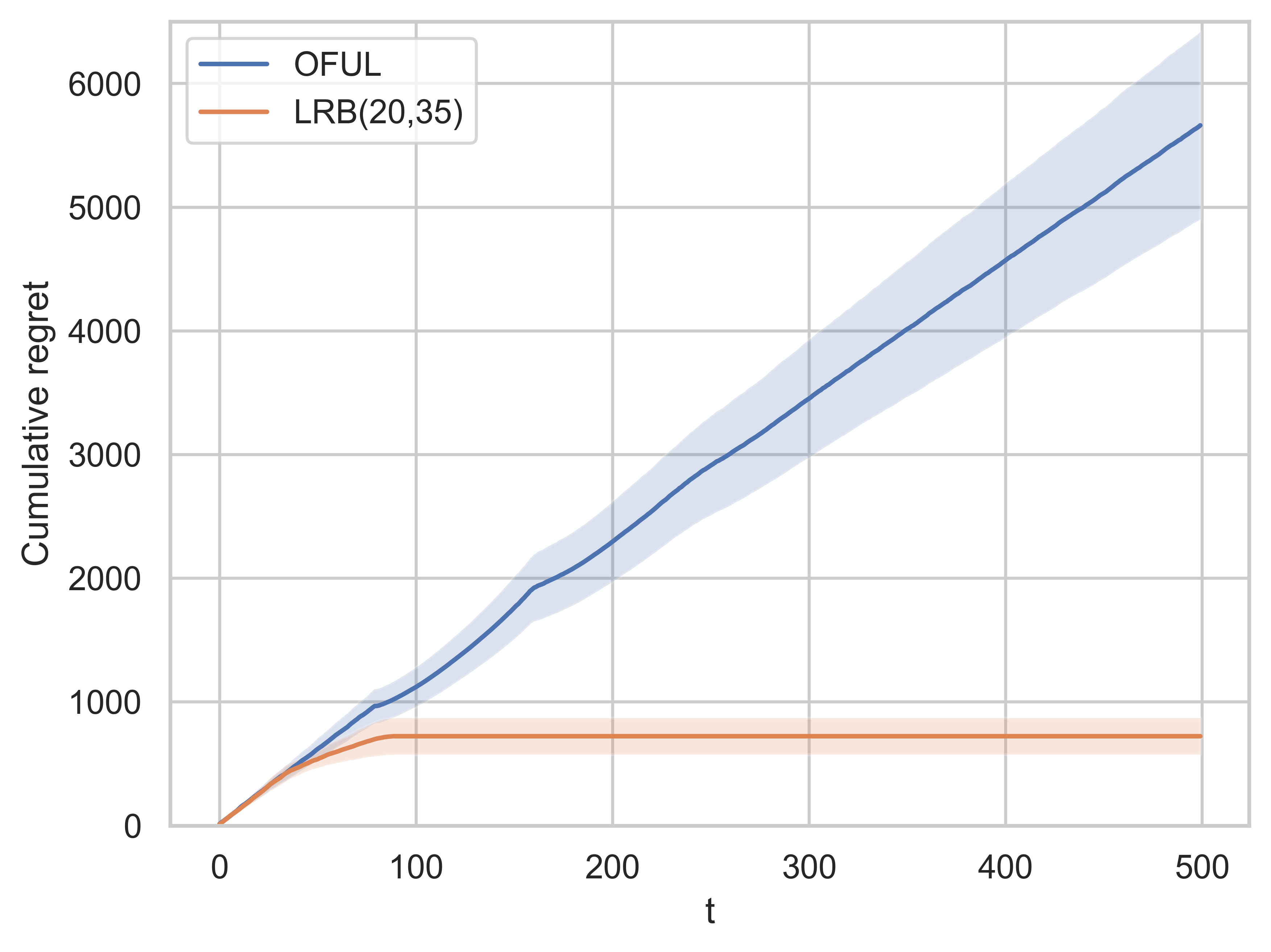
(a)

(b)

Figure 3: Regrets of OFUL and LRB under the contextual setting. Panel 3(a) shows confidence intervals for the cumulative regret of OFUL Algorithm from Abbasi-Yadkori et al. (2011) and LRB (Algorithm 1) with ($h$,$f$) = ($20$,$35$) as functions of time, and panel 3(b) shows average cumulative regrets of the LRB Algorithm 1 at different combinations of number of forced samples $f$ and filtering resolution $h$.

6 Conclusion

This paper introduced a new approach that reduces the opportunity cost of online experimentation for finding the best product from a large product set. We achieved such goals by lowering the cost incurred in the burn-in period and overcoming the cold-start problem. We first identified that many products can be viewed as two-sided products. Then we formulated the problem as a stochastic bandit problem with many arms, where each arm corresponds to a version of the two-sided product. We shaped the rewards of the products into a matrix format and proposed the Low-Rank Bandit algorithm, an efficient algorithm whose gap-dependent regret bound scales with the sum of the number of choices for the first side and the number of choices for the second side theoretically, rather than the total number of versions in the existing literature, which is orders of magnitude improvement.

We empirically demonstrated that the Low-Rank Bandit is more versatile than existing methods: it can adjust to different lengths of the time horizon by modifying the size of the submatrix it works with. We illustrated the Low-Rank Bandit’s practical relevance by evaluating it on an advertisement targeting problem for a music streaming service. We found that it surpasses existing bandit methods to target the right segment of the user population and the creator population, largely reduces the cost of experimentation and expedites the process. It is noteworthy that we also came up with a low-rank reduction model for contextual bandits, under which we showed our algorithm’s superior performance in cost reduction than a classical contextual bandit algorithm. We conclude by discussing some directions for future endeavor.

Future directions.

First, in certain applications, more dimensions can be used to characterize a product. For example, Airbnb Experiences can be modeled as three-sided products in the following manner. Besides the content and the location of one activity, we can leverage its temporal side as well. Thus, how to deal with multi-sided products remains a promising future direction.

On a related note, for settings such as Stitch Fix personalized styling, we have a unique reward profile for each user. Different user reward profiles might share similarity. How to leverage information among different users is also an exciting next step: learning reward matrix on one two-sided product for a user will help us understand the reward matrix (even on other two-sided products) for other users better.

For the two points we have discussed so far, the data can be shaped into a tensor. Thus, literature on tensor-shaped data and tensor completion may shed light on possible solutions.

In addition, it would be interesting to tackle the following related scenario: we have users and products as rows and columns, upon a user’s arrival, we want to recommend a product (or an array of products) he/she likes the best. We do this experiment in an online fashion and our goal is to find the product(s) that each user likes the best. This is a classical product assortment problem. The question is how to leverage the low-rank structure to expedite the experiment.

Finally, our work also taps into the field of product bundling (Stigler 1963), since two-sided products can be viewed as a bundle between the two sides. Canonical works such as Adams and Yellen (1976), Schmalensee (1984), McAfee et al. (1989) focus on the basic two-product case. Our work gives new perspectives on how to leverage potential low-rank matrix structure. For instance, we can shape the bundling data into a matrix whose entries are the expected rewards or purchase probabilities of bundles of two products. Through customer’s purchase behaviors, the preference regarding each bundle can be learned, which can inform the pricing scheme.

7 Row Enhancement Procedure

Note that the bound in Assumption 3.2 gives matrix-wise estimation error, and it does not characterize how this error is distributed across different entries. Using matrix-wise estimation error to bound entry-wise estimation error is rather loose. Instead, we use row-wise estimation error, derived from a row enhancement procedure adapted from Hamidi et al. (2019), to bound the entry-wise estimation error.

To be more specific, the trivial inequality $\|\bar{\operatorname{\mathbf{B}}}_{j}-\operatorname{\mathbf{B}}^{*}_{j}\|_{2}\leq\|\bar{\operatorname{\mathbf{B}}}-\operatorname{\mathbf{B}}^{*}\|_{F}$ would introduce an unnecessary $\sqrt{d_{r}}$ factor when bounding the row-wise estimation error. With the row-enhancement procedure described in Algorithm 3, such row-wise error bound can be improved. Specifically, let $\mathcal{J}=\{t_{1},\ldots,t_{n}\}$ be a given set of $n$ time periods with $t_{1}<t_{2}<\cdots<t_{n}$. In Algorithm 3, the data is split into two halves $\mathcal{J}_{1}=\{t_{1},\ldots,t_{\frac{n}{2}}\}$ and $\mathcal{J}_{2}=\{t_{\frac{n}{2}+1},\ldots,t_{n}\}$. The first portion, indexed by $\mathcal{J}_{1}$, will be fed to a low-rank estimator and the result is denoted by $\bar{\operatorname{\mathbf{B}}}(\mathcal{J}_{1})$. The second portion, indexed by $\mathcal{J}_{2}$, is then used to “enhance” each row of $\bar{\operatorname{\mathbf{B}}}(\mathcal{J}_{1})$. The final output is then denoted by $\hat{\operatorname{\mathbf{B}}}(\mathcal{J})$. The enhanced row-wise error bound is characterized by Proposition 8.5.

Algorithm 3 Row-Enhancement Procedure

1:Input: Low-rank matrix estimator $\bar{\operatorname{\mathbf{B}}}\in\mathbb{R}^{d_{r}\times d_{c}}$, $\mathcal{J}=\{t_{1},\dots,t_{n}\}$, and observations $(\operatorname{\mathbf{X}}^{\pi}_{t_{1}},y_{t_{1}}),\dots,(\operatorname{\mathbf{X}}^{\pi}_{t_{n}},y_{t_{n}})$

2:Initialize $\widehat{\operatorname{\mathbf{B}}}\in\mathbb{R}^{d_{r}\times d_{c}}$

3:Split $\mathcal{J}$ into $\mathcal{J}_{1}=\{t_{1},\dots,t_{\frac{n}{2}}\}$ and $\mathcal{J}_{2}=\{t_{\frac{n}{2}+1},\dots,t_{n}\}$

4:Compute singular value decomposition (SVD): $\bar{\operatorname{\mathbf{B}}}(\mathcal{J}_{1})=\operatorname{\mathbf{U}}\operatorname{\mathbf{D}}\operatorname{\mathbf{V}}^{\top}$

5:Let $\operatorname{\mathbf{V}}_{r}$ be the matrix containing first $\mathfrak{r}$ columns of $\operatorname{\mathbf{V}}$

6:for $j=1,2,\dots,d_{r}$ do

7:     Let $\hat{\vartheta}_{j}=\argmin_{\vartheta\in\mathbb{R}^{r}}\sum_{t_{i}\in\mathcal{J}_{2}^{j}}\left(y_{t_{i}}-[\operatorname{\mathbf{V}}_{r}\vartheta]_{t_{i}}\right)^{2}$

8:     Set row $j$ of $\widehat{\operatorname{\mathbf{B}}}$ to $(\operatorname{\mathbf{V}}_{r}\hat{\vartheta}_{j})^{\top}$

9:end for

10:return $\widehat{\operatorname{\mathbf{B}}}$

8 Proof for Row-Wise Guarantees of Forced-Sample Estimator

We introduce two lemmas which lead to the proof of row-wise guarantees in Lemma 3.4.

Lemma 8.1 (Lemma 1 in Hamidi et al. (2019))

The forced-sampling sets created by the forced sampling rule (3.1) satisfy the following inequalities, for all $t\geq 2\rho\log(\rho)$, provided that $\rho\geq 24$,

$$\mathbb{P}\big{(}|\mathcal{F}_{t}|\geq 6\rho\log(t)\big{)}\leq t^{-1}\quad\text{ and }\quad\mathbb{P}\big{(}|\mathcal{F}_{t}|\leq\rho\log(t)/2\big{)}\leq t^{-3}.$$

Proof 8.2

Proof of Lemma 8.1. Let $a:=2\rho\lfloor\log(\rho)\rfloor$. We have that

$$\theta: =\mathbb{E}[|\mathcal{F}_{t}|]=a+\sum_{i=a+1}^{t}\frac{\rho}{i-\rho\log(\rho)+1}$$

$$\leq a+\rho(\log(t-a)+1)$$

$$\leq 3\rho\log(t).$$

Similarly, we get that

$$\theta\geq a+\rho\log(t-\rho\log(\rho))\geq\rho\log(t).$$

Applying Chernoff inequality, we get that

$$\mathbb{P}(|\mathcal{F}_{t}|\geq 6\rho\log(t)) \leq\mathbb{P}(|\mathcal{F}_{t}|\geq 2\theta)$$

$$\leq\exp(-\frac{\theta}{3})$$

$$\leq\frac{1}{t}.$$

The other inequality can be obtained by applying lower tail Chernoff bound:

$$\mathbb{P}\Bigg{(}|\mathcal{F}_{t}|\leq\frac{\rho\log(t)}{2}\Bigg{)} \leq\mathbb{P}\left(|\mathcal{F}_{t}|\leq\frac{\theta}{2}\right)$$

$$\leq\exp\left(-\frac{\theta}{8}\right)$$

$$\leq\frac{1}{t^{3}}.$$

The last step follows because

$$\exp\left(-\frac{\theta}{8}\right)\leq\exp\left(-\frac{\rho\log(t)}{8}\right)\leq\exp(-3\log t)=\exp(\log(t^{-3}))=\frac{1}{t^{3}}.$$

 $\square$

Lemma 8.3 (Lemma 2 in Hamidi et al. (2019))

Let $\mathcal{I}$ be a (deterministic) subset of the forced-sampling observations, and by $\mathcal{I}_{j}\subseteq\mathcal{I}$, we denote the observations corresponding to row $j\in[d_{r}]$. Then, the following inequality holds,

$$\mathbb{P}\Bigg{(}\frac{|\mathcal{I}_{j}|}{|\mathcal{I}|}\leq\frac{1}{2d_{r}}\biggm{|}|\mathcal{I}|\Bigg{)}\leq\exp\Bigg{[}-\frac{|\mathcal{I}|}{8d_{r}}\Bigg{]}.$$

Proof 8.4

Proof of Lemma 8.3. We use Chernoff bound to prove this result. Note that, in the pure exploration phase, there is an equal chance of selecting each row. Therefore, conditional on the size of $\mathcal{I}$, the size of $\mathcal{I}_{j}$ is a binomial random variable with $\frac{1}{d_{r}}$ probability of success and $|\mathcal{I}|$ trials. To be more specific, we apply the lower tail Chernoff bounds $\mathbb{P}(\frac{|\mathcal{I}_{j}|}{|\mathcal{I}|}\leq(1-\delta)\mu)\leq e^{-\mu\delta^{2}/2}$ with $\delta=\frac{1}{2},\mu=\frac{|\mathcal{I}|}{d_{r}}$.  $\square$

Proposition 8.5 (Adapted from Hamidi et al. (2019). We refer to their paper for the proof)

Fix $\delta>0$. Suppose $(n/\log n)\geq\alpha_{2}(1+\delta^{-2})\mathfrak{r}(d_{r}+d_{c})$ and Assumption 3.2 holds. Also, for all $j\in[d_{r}]$, assume that the observation sets $\mathcal{J}_{1}^{j}$ and $\mathcal{J}_{2}^{j}$ each consists of $n$ independent observations (notation defined in Appendix 7). Then the inequalities

$$\|\widehat{\operatorname{\mathbf{B}}}_{j}(\mathcal{J})-\operatorname{\mathbf{B}}^{*}_{j}\|_{2}\leq 16\sqrt{\frac{\mathfrak{r}}{d_{r}}}\cdot\mu(\operatorname{\mathbf{B}}^{*})\cdot\delta\quad\text{for all $j\in[d_{r}]$}$$

hold simultaneously with probability at least

$$1-\mathbb{P}(\|\bar{\operatorname{\mathbf{B}}}(\mathcal{J}_{1})-\operatorname{\mathbf{B}}^{*}\|_{F}\geq\delta)-4d_{r}\cdot\exp(-\alpha_{3}n)-\mathfrak{r}d_{r}\cdot\exp\Big{(}-\frac{\delta n\mu(\operatorname{\mathbf{B}}^{*})^{2}}{d_{r}d_{c}}\Big{)},$$

where $\alpha_{3}$ is a constant.

Equipped with Proposition 8.5, we are ready to prove Lemma 3.4 below.

Proof 8.6

Proof of Lemma 3.4.

Let $\mathcal{J}_{1}$ and $\mathcal{J}_{2}$ be the first and second half of $\mathcal{F}_{t}$ respectively. Let $n$ denote the size of $\mathcal{F}_{t}$. Let $n_{l,j}$ for $l\in\{1,2\}$ and $j\in[d_{r}]$ denote the number of times row $j$ appears in $\mathcal{J}_{l}$.

When $n\geq\rho\log(t)/2$, we have $\frac{\rho\log(t)}{8d_{r}}\leq\frac{n}{4d_{r}}$, so that

$$\mathbb{P}\left(n_{l,j}\leq\frac{\rho\log(t)}{8d_{r}}\right)\leq\mathbb{P}\left(n_{l,j}\leq\frac{n}{4d_{r}}\right).$$

Using Lemma 8.3, we get

$$\mathbb{P}\left(n_{l,k}\leq\frac{n}{4d_{r}}\right)\leq\exp\left(-\frac{n/2}{8d_{r}}\right)=\exp\left(-\frac{n}{16d_{r}}\right)\leq\exp\left(-\frac{\rho d_{r}\log(t)}{16d_{r}}\right)\leq\exp\left(-\frac{64d_{r}\log(t)}{16d_{r}}\right)\leq\frac{1}{t^{4}},$$

provided that $\rho\geq 32$.

It follows from the union bound, Lemma 8.1 and Lemma 8.3 that for all $t\geq 2\rho\log(\rho)$, we have

$$\mathbb{P}\Bigg{(}\exists(l,j)\in\{1,2\}\times[d_{r}]:n_{l,j}\leq\frac{\rho\log(t)}{8d_{r}}\Bigg{)}$$

$$\leq \mathbb{E}\Bigg{[}\operatorname{\mathbb{I}}\left(\exists(l,j)\in\{1,2\}\times[d_{r}]:n_{l,j}\leq\frac{\rho\log(t)}{8d_{r}}\right)\cdot\operatorname{\mathbb{I}}\big{(}n\geq\rho\log(t)/2\big{)}\Bigg{]}+\mathbb{E}\Bigg{[}\operatorname{\mathbb{I}}\big{(}n<\rho\log(t)/2\big{)}\Bigg{]}$$

$$\leq \sum_{(l,j)}\mathbb{P}\left(n_{l,j}\leq\frac{n}{4d_{r}}\right)+\frac{1}{t^{3}}$$

$$\leq \frac{2d_{r}}{t^{4}}+\frac{1}{t^{3}}\leq\frac{3}{t^{3}},$$ (8.1)

where the second equality follows from $\mathbb{P}\Big{(}n<\rho\log(t)\Big{)}\leq 1/t^{3}$ by Lemma 8.1.

Next, note that all the samples in $\mathcal{F}_{t}$ are independent of each other. Therefore, the assumptions of Proposition 8.5 hold. Let $\rho\geq\frac{\alpha_{4}}{\delta^{2}}$ where $\alpha_{4}=\frac{3\mathfrak{r}(d_{r}+d_{c})}{\alpha_{1}}$, Assumption 3.2 suggests that when $n/2\geq\rho\log(t)/2$, it holds that

$$\mathbb{P}(\|\bar{\operatorname{\mathbf{B}}}^{F}(\mathcal{J})-\operatorname{\mathbf{B}}^{*}\|_{F}\geq\delta)\leq\frac{1}{t^{3}}.$$ (8.2)

The detail for showing this is below. When $\rho\geq\alpha_{4}/\delta^{2}$, it holds that $3\log t\frac{(d_{r}+d_{c})\mathfrak{r}}{\alpha_{1}\delta^{2}}\leq\rho\log t\leq n$. (8.2) then follows from Assumption 3.2.

Recall that

$$\gamma(h):=\sqrt{\frac{d_{r}}{\mathfrak{r}}}\cdot\frac{h}{64\mu^{*}}.$$

Then, plugging in $\delta=\gamma(h)$, Proposition 8.5 yields

$$\mathbb{P}\Bigg{(}\exists j:\|\hat{\operatorname{\mathbf{B}}}_{j}^{F}(\mathcal{J})-\operatorname{\mathbf{B}}^{*}_{j}\|_{2}\geq\frac{h}{4}\Bigg{)}\leq\frac{9}{t^{3}}.$$

In the above, we have used $\rho\geq 32d_{r}/\alpha_{3}$ and $n_{l,j}\geq\frac{\rho\log(t)}{8d_{r}}$ from 8.1 to get

$$4d_{r}\exp(-\alpha_{3}n_{l,j})\leq 4d_{r}\exp\Bigg{(}-\frac{\alpha_{3}\rho\log(t)}{8d_{r}}\Bigg{)}\leq\frac{4d_{r}}{t^{4}}\leq\frac{4}{t^{3}},$$ (8.3)

and $\rho\geq\alpha_{5}/h$ where $\alpha_{5}=1280d_{c}\sqrt{d_{r}\mathfrak{r}}/\mu^{*}$ to get

$$\mathfrak{r}d_{r}\cdot\exp\Bigg{(}-\frac{\delta\mu^{*}{{}^{2}}\rho\log(t)}{4d_{r}d_{c}}\Bigg{)}\leq\mathfrak{r}d_{r}\cdot\exp(-5\log(t))\leq\frac{1}{t^{3}}.$$ (8.4)

Combining (8.1), (8.2), (8.3) and (8.4), we get the claimed $9/t^{3}$ bound.  $\square$

9 Proofs for Cumulative Regret

9.1 Key Steps of the Regret Analysis

Let $t_{0}$ be the initial forced-sampling periods, determined by $2\rho\log(\rho)$ in (3.1). The key idea is to decompose the regret into three parts:

1. Initialization ($t\leq t_{0}$), and other forced sampling rounds.

2. Times $t>t_{0}$ when the event $G(\mathcal{F}_{t})$ does not hold.

3. Times $t>t_{0}$ when the event $G(\mathcal{F}_{t})$ holds but the Low-Rank Bandit plays a suboptimal arm chosen by the UCB algorithm from the targeted set $\mathcal{C}$.

The cumulative expected regret from pure exploration (part (a)) at time $T$ is bounded by at most $2b^{*}(t_{0}+6\rho\log T)$ (Lemma 9.1). This follows from the fact that the worst-case regret at any time step is at most $2b^{*}$ (Assumption 2.1), while there are only $t_{0}$ initialization samples and at most $6\rho\log T$ forced samples up to time $T$ (Lemma 8.1).

Next, the cumulative expected regret from part (b) where $G(\mathcal{F}_{t})$ does not hold is bounded by at most $20b^{*}\log(T)$ (Lemma 9.3). This follows from the tail inequality for the forced-sample estimator (Lemma 3.4), which bounds the probability that event $G(\mathcal{F}_{t})$ does not hold at time $t$ by at most $10/{t^{3}}$. The result follows from summing this quantity over time periods $t_{0}<t\leq T$.

Finally, the gap-dependent bound and the gap-independent bound differ in the derivation of the cumulative expected regret from part (c). This is bounded by at most ${8g(h)\log T}{\Delta^{-1}}+[1+{\pi^{2}}/{3}]2hg(h)$ for the gap-dependent bound (Lemma 9.5) and by at most $4\sqrt{2Tg(h)\log(T)}+(1+\frac{\pi^{2}}{3})\sum_{(j,k)\in\mathcal{S}_{opt}}\Delta_{jk}$ for the gap-independent bound (Lemma 9.7). To show this, we first observe that if event $G(\mathcal{F}_{t})$ holds, then the set $\mathcal{C}$ (chosen by the forced-sample estimator) contains the optimal arm $(j^{*},k^{*})=\argmax_{(j,k)\in[d_{r}]\times[d_{c}]}\operatorname{\mathbf{B}}^{*}_{jk}$ and no sub-optimal arms from the set $\mathcal{S}_{sub}$ (Lemma 9.11). Then the UCB subroutine will work with $g(h)$ number of near-optimal arms and pick the best among them as the arm for the current round.

Summing up the regret contributions from all parts gives us our main result.

9.2 Part (a)

Lemma 9.1

$$\textnormal{{Regret}}_{T}^{(a)}\leq 2b^{*}\mathbb{E}[t_{0}+|\mathcal{F}_{T}|]\leq 2b^{*}(t_{0}+6\rho\log T).$$ (9.1)

Proof 9.2

Proof for Lemma 9.1.

Note that, for each suboptimal choice, the regret incurred at each step is at most $\operatorname{\mathbf{B}}^{*}_{j^{*}k^{*}}-\operatorname{\mathbf{B}}^{*}_{jk}$ for some $(j,k)$. In addition, since $\|\operatorname{\mathbf{B}}^{*}\|_{\infty,2}\leq b^{*}$, then we must have $\|\operatorname{\mathbf{B}}^{*}\|_{\infty}\leq b^{*}$. In turn, we have

$$\operatorname{\mathbf{B}}^{*}_{j^{*}k^{*}}-\operatorname{\mathbf{B}}^{*}_{jk}\leq|\operatorname{\mathbf{B}}^{*}_{j^{*}k^{*}}-\operatorname{\mathbf{B}}^{*}_{jk}|\leq|\operatorname{\mathbf{B}}^{*}_{j^{*}k^{*}}|+|\operatorname{\mathbf{B}}^{*}_{jk}|\leq 2b^{*}.$$

Next, the number of times that each suboptimal arm is pulled is less than or equal to $t_{0}+|\mathcal{F}_{T}|$. Putting together and using Lemma 8.1, we get

$$\textnormal{{Regret}}_{T}^{(a)}\leq 2b^{*}\mathbb{E}[t_{0}+|\mathcal{F}_{T}|]\leq 2b^{*}(t_{0}+6\rho\log T).$$ (9.2)

 $\square$

9.3 Part (b)

Lemma 9.3

$$\textnormal{{Regret}}_{T}^{(b)}\leq 100b^{*}.$$ (9.3)

Proof 9.4

Proof for Lemma 9.3. Next, it follows from the definition of $G(\mathcal{F}_{t})$ and Lemma 3.4 that the number of times that $G(\mathcal{F}_{t})=0$ is controlled by

$$\mathbb{E}\Bigg{[}\sum_{t=t_{0}+1}^{T}[1-G(\mathcal{F}_{t})]\Bigg{]}=\sum_{t=t_{0}+1}^{T}\mathbb{P}(G(\mathcal{F}_{t})=0)\leq\sum_{t=t_{0}+1}^{T}9t^{-3}\leq 15.$$

During the rounds that $G(\mathcal{F}_{t})=0$, it is not guaranteed that the best arm is selected into the targeted set (according to Lemma 9.11). For these rounds, the regret incurred can be decomposed into two parts (part 1(ii) and part 2(i) as we define $\phi_{1}$ and $\phi_{2}$ in Section 3.5): (1) the gap between the best arm in the targeted set and the best arm in the entire arm set; (2) the regret incurred by UCB routine for not selecting the best arm in the targeted set. (1) can be bounded by $2b^{*}$ and (2) can be bounded by $2b^{*}$.

Hence, $\textnormal{{Regret}}_{T}^{(b)}\leq(2b^{*}+2b^{*})\mathbb{E}\Bigg{[}\sum_{t=t_{0}+1}^{T}[1-G(\mathcal{F}_{t})]\Bigg{]}$, we have

$$\textnormal{{Regret}}_{T}^{(b)}\leq 100b^{*}.$$ (9.4)

 $\square$

9.4 Gap-Dependent Bound for Part (c)

As mentioned before, to bound part (c) in the cumulative regret, we build on the standard proof for the UCB algorithm (Lattimore and Szepesvári 2020, Chapter 7), with the help from Lemma 9.11. Under the condition for Lemma 9.11, the biggest entry is for sure in the targeted set $\mathcal{C}$. So we only incur a cost when some element in $\mathcal{S}_{opt}^{h}$ other than the biggest entry is selected. Further, since $g(h)=|\mathcal{S}_{opt}^{h}|$, we can use $g(h)$ as an upper bound on the number of arms in the targeted set $\mathcal{C}$. We first show the gap-dependent bound for part (c).

Lemma 9.5

$$\textnormal{{Regret}}_{T}^{(c)} \leq\frac{8g(h)\log T}{\Delta}+\Bigg{(}1+\frac{\pi^{2}}{3}\Bigg{)}hg(h).$$ (9.5)

Proof 9.6

Proof of Lemma 9.5. We start by finding a bound on the number of times each non-best entry in $\mathcal{S}^{h}_{opt}$ is pulled when $G(\mathcal{F}_{t})=1$. Let $\xi_{(j,k)}(n)$ denote the number of times we have played action $(j,k)\in\mathcal{S}^{h}_{opt}$ in rounds $1\leq t\leq n$ when $G(\mathcal{F}_{t})=1$. Let $\xi^{A}_{(j,k)}(n)$ denote the total number of times we have played action $(j,k)$ in rounds $1\leq t\leq n$. Let $a(y,T)=\sqrt{2\log T/y}$. We know that, for some arbitrary $m\geq 0$,

$$\xi_{(j,k)}(T)=\sum_{t=1}^{T}\mathbb{I}\Big{(}(j_{t},k_{t})=(j,k)\text{ and }G(\mathcal{F}_{t})=1\Big{)} \leq m+\sum_{t=1}^{T}\mathbb{I}\Big{(}(j_{t},k_{t})=(j,k)\text{ and }\xi_{(j,k)}(t-1)\geq m\Big{)}$$

$$\leq m+\sum_{t=1}^{T}\mathbb{I}\Big{(}(j_{t},k_{t})=(j,k)\text{ and }\xi^{A}_{(j,k)}(t-1)\geq m\Big{)}.$$

Since $G(\mathcal{F}_{t})=1$, we must have $(j^{*},k^{*})$ in the targeted set $\mathcal{C}(t)$ by Lemma 9.11. Therefore, when $(j,k)$ is pulled at $t$ when $G(\mathcal{F}_{t})=1$, we must have

$$\bar{x}_{(j,k)}+a(\xi^{A}_{(j,k)}(t),t-1)\geq\bar{x}^{*}+a(\xi^{A}_{(j^{*},k^{*})}(t),t-1)$$

Therefore, we arrive at

$$\xi_{(j,k)}(T)\leq m+\sum_{t=1}^{T}\mathbb{I}\Big{(}\bar{x}_{(j,k)}+a(\xi^{A}_{(j,k)}(t),t-1)\geq\bar{x}^{*}+a(\xi^{A}_{(j^{*},k^{*})}(t),t-1)\text{ and }\xi^{A}_{(j,k)}(t-1)\geq m\Big{)}.$$

Denote by $\bar{x}_{(j,k),s}$ the random variable for the empirical mean after playing action $(j,k)$ a total of $s$ times, and $\bar{x}^{*}_{s}$ the corresponding quantity for the best entry. Then we must have

$$\xi_{(j,k)}(T)\leq m+\sum_{t=1}^{T}\mathbb{I}\Big{(}\max_{m\leq s<t}\bar{x}_{(j,k),s}+a(s,t-1)\geq\min_{0<s^{\prime}<t}\bar{x}^{*}_{s^{\prime}}+a(s^{\prime},t-1)\text{ and }\xi^{A}_{(j,k)}(t-1)\geq m\Big{)}.$$

It follows that

$$\xi_{(j,k)}(T)\leq m+\sum_{t=1}^{T}\sum_{s=m}^{t-1}\sum_{s^{\prime}=1}^{t-1}\mathbb{I}\Big{(}\bar{x}_{(j,k),s}+a(s,t-1)\geq\bar{x}^{*}_{s^{\prime}}+a(s^{\prime},t-1)\Big{)}.$$

So,

$$\xi_{(j,k)}(T)\leq m+\sum_{t=1}^{\infty}\sum_{s=m}^{t}\sum_{s^{\prime}=1}^{t}\mathbb{I}\Big{(}\bar{x}_{(j,k),s}+a(s,t)\geq\bar{x}^{*}_{s^{\prime}}+a(s^{\prime},t)\Big{)}.$$

Suppose that the event $\bar{x}_{(j,k),s}+a(s,t)\geq\bar{x}^{*}_{s^{\prime}}+a(s^{\prime},t)$ happens. Then we claim that at least one of the following events must happen:

1. $\bar{x}^{*}_{s^{\prime}}\leq\operatorname{\mathbf{B}}^{*}_{j^{*}k^{*}}-a(s^{\prime},t)$,

2. $\bar{x}_{(j,k),s}\geq\operatorname{\mathbf{B}}^{*}_{jk}+a(s,t)$,

3. $\operatorname{\mathbf{B}}^{*}_{j^{*}k^{*}}<\operatorname{\mathbf{B}}^{*}_{jk}+2a(s,t)$.

We prove this claim by contradiction. Suppose that none of the three events are true. Then we have

$$\bar{x}_{(j,k),s}+a(s,t)\geq\bar{x}^{*}_{s^{\prime}}+a(s^{\prime},t)>\operatorname{\mathbf{B}}^{*}_{j^{*}k^{*}}-a(s^{\prime},t)+a(s^{\prime},t)=\operatorname{\mathbf{B}}^{*}_{j^{*}k^{*}}$$

and

$$\operatorname{\mathbf{B}}^{*}_{jk}+2a(s,t)>\bar{x}_{(j,k),s}+a(s,t).$$

Putting the above two inequalities together, we get $\operatorname{\mathbf{B}}^{*}_{j^{*}k^{*}}<\operatorname{\mathbf{B}}^{*}_{jk}+2a(s,t)$. Here we reached a contradiction as this is exactly event 3. So we conclude that at least one of the three events is true.

Note that, if we take $m=8\log T/(\operatorname{\mathbf{B}}^{*}_{j^{*}k^{*}}-\operatorname{\mathbf{B}}^{*}_{jk})^{2}$, then $2a(s,t)\leq\operatorname{\mathbf{B}}^{*}_{j^{*}k^{*}}-\operatorname{\mathbf{B}}^{*}_{jk}$ for any $s\geq m$. Hence, $\operatorname{\mathbf{B}}^{*}_{j^{*}k^{*}}-\operatorname{\mathbf{B}}^{*}_{jk}-2a(s,t)\geq 0$. So when $m=8\log T/(\operatorname{\mathbf{B}}^{*}_{j^{*}k^{*}}-\operatorname{\mathbf{B}}^{*}_{jk})^{2}$, the probability that at least one of the three events above happens is $2t^{-4}$. This is based on the Chernoff-Hoeffding inequality that $\mathbb{P}\Big{(}\bar{x}_{(j,k),s}\geq\operatorname{\mathbf{B}}^{*}_{jk}+a(s,t)\Big{)}\leq t^{-4}$ and $\mathbb{P}\Big{(}\bar{x}^{*}_{s^{\prime}}\leq\operatorname{\mathbf{B}}^{*}_{j^{*}k^{*}}-a(s^{\prime},t)\Big{)}\leq t^{-4}$. Therefore,

$$\mathbb{E}[\xi_{(j,k)}(T)] \leq m+\sum_{t=1}^{\infty}\sum_{s=m}^{t}\sum_{s^{\prime}=1}^{t}\mathbb{P}\Big{(}\bar{x}_{(j,k),s}+a(s,t)\geq\bar{x}^{*}_{s^{\prime}}+a(s^{\prime},t)\Big{)}$$

$$\leq\frac{8\log T}{(\operatorname{\mathbf{B}}^{*}_{j^{*}k^{*}}-\operatorname{\mathbf{B}}^{*}_{jk})^{2}}+\sum_{t=1}^{\infty}\sum_{s=m}^{t}\sum_{s^{\prime}=1}^{t}2t^{-4}$$

$$\leq\frac{8\log T}{(\operatorname{\mathbf{B}}^{*}_{j^{*}k^{*}}-\operatorname{\mathbf{B}}^{*}_{jk})^{2}}+1+\sum_{t=1}^{\infty}\sum_{s=m}^{t}\sum_{s^{\prime}=1}^{t}2t^{-4}$$

$$\leq\frac{8\log T}{(\operatorname{\mathbf{B}}^{*}_{j^{*}k^{*}}-\operatorname{\mathbf{B}}^{*}_{jk})^{2}}+1+2\sum_{t=1}^{\infty}t^{-2}$$

$$\leq\frac{8\log T}{(\operatorname{\mathbf{B}}^{*}_{j^{*}k^{*}}-\operatorname{\mathbf{B}}^{*}_{jk})^{2}}+1+\frac{\pi^{2}}{3}.$$ (9.6)

It follows that

$$\textnormal{{Regret}}_{T}^{(c)} =\sum_{(j,k)\in\mathcal{S}_{opt}^{h}}(\operatorname{\mathbf{B}}^{*}_{j^{*}k^{*}}-\operatorname{\mathbf{B}}^{*}_{jk})\mathbb{E}[\xi_{(j,k)}(T)]$$

$$\leq\sum_{(j,k)\in\mathcal{S}_{opt}^{h}}\Bigg{[}\frac{8\log T}{\operatorname{\mathbf{B}}^{*}_{j^{*}k^{*}}-\operatorname{\mathbf{B}}^{*}_{jk}}+\Bigg{(}1+\frac{\pi^{2}}{3}\Bigg{)}(\operatorname{\mathbf{B}}^{*}_{j^{*}k^{*}}-\operatorname{\mathbf{B}}^{*}_{jk})\Bigg{]}$$

$$\leq\sum_{(j,k)\in\mathcal{S}_{opt}^{h}}\Bigg{[}\frac{8\log T}{\Delta}+\Bigg{(}1+\frac{\pi^{2}}{3}\Bigg{)}h\Bigg{]}$$

$$\leq\frac{8g(h)\log T}{\Delta}+\Bigg{(}1+\frac{\pi^{2}}{3}\Bigg{)}hg(h).$$

 $\square$

9.5 Gap-Independent Bound for Part (c)

Now we tackle the gap-independent bound for part (c).

Lemma 9.7

let $\Delta_{jk}=\operatorname{\mathbf{B}}^{*}_{j^{*}k^{*}}-\operatorname{\mathbf{B}}^{*}_{jk}$, for any given $(j,k)$,

$$R_{T}^{(c)} \leq 4\sqrt{2Tg(h)\log(T)}+(1+\frac{\pi^{2}}{3})\sum_{(j,k)\in\mathcal{S}_{opt}^{h}}\Delta_{jk}.$$ (9.7)

Proof 9.8

Proof for Lemma 9.7 (Adapted from proof of Theorem 7.2 in Lattimore and Szepesvári (2020)). From (9.6), we have the following inequality:

$$\mathbb{E}[\xi_{(j,k)}(T)] \leq\frac{8\log T}{(\operatorname{\mathbf{B}}^{*}_{j^{*}k^{*}}-\operatorname{\mathbf{B}}^{*}_{jk})^{2}}+1+\frac{\pi^{2}}{3}.$$

Therefore, using the basic regret decomposition, we have

$$R_{T}^{(c)} =\sum_{(j,k)\in\mathcal{S}_{opt}^{h}}(\operatorname{\mathbf{B}}^{*}_{j^{*}k^{*}}-\operatorname{\mathbf{B}}^{*}_{jk})\mathbb{E}[\xi_{(j,k)}(T)]$$

$$=\sum_{(j,k)\in\mathcal{S}_{opt}^{h},\Delta_{jk}\leq\chi}\Delta_{jk}\mathbb{E}[\xi_{(j,k)}(T)]+\sum_{(j,k)\in\mathcal{S}_{opt}^{h},\Delta_{jk}\geq\chi}\Delta_{jk}\mathbb{E}[\xi_{(j,k)}(T)]$$

$$\leq T\chi+\sum_{(j,k)\in\mathcal{S}_{opt}^{h},\Delta_{jk}\geq\chi}\Bigg{(}\frac{8\log T}{\Delta_{jk}}+\Delta_{jk}(1+\frac{\pi^{2}}{3})\Bigg{)}$$

$$\leq T\chi+\frac{8g(h)\log T}{\chi}+(1+\frac{\pi^{2}}{3})\sum_{(j,k)\in\mathcal{S}_{opt}^{h}}\Delta_{jk}$$

$$\leq 4\sqrt{2Tg(h)\log(T)}+(1+\frac{\pi^{2}}{3})\sum_{(j,k)\in\mathcal{S}_{opt}^{h}}\Delta_{jk},$$

where we choose $\chi=\sqrt{8g(h)\log(T)/T}$.  $\square$

9.6 Proofs for Theorem 3.5 and 3.6

Proof 9.9

Proof of Theorem 3.5. Combining Lemmas 9.1-9.5, and by plugging in $\rho=2\alpha_{2}[1+{\gamma(h)^{-2}}]r(d_{r}+d_{c})$, the cumulative regret is as (3.2). Specifically,

$$\textnormal{{Regret}}_{T}(h) \leq\overbrace{2b^{*}(t_{0}+6\rho\log T)}^{\text{Regret from (a)}}+\overbrace{100b^{*}}^{\text{Regret from (b)}}+\overbrace{\frac{8g(h)\log T}{\Delta}+\Bigg{(}1+\frac{\pi^{2}}{3}\Bigg{)}hg(h)}^{\text{Regret from (c)}}$$

$$=b^{*}\Big{[}2t_{0}+24\alpha_{2}(1+\frac{1}{\gamma(h)^{2}})\mathfrak{r}(d_{r}+d_{c})\log T\Big{]}+100b^{*}+\frac{8g(h)\log T}{\Delta}+\Bigg{(}1+\frac{\pi^{2}}{3}\Bigg{)}hg(h)$$

$$\leq b^{*}\Big{[}2t_{0}\alpha_{2}(1+\frac{1}{\gamma(h)^{2}})\mathfrak{r}(d_{r}+d_{c})\log T+24\alpha_{2}(1+\frac{1}{\gamma(h)^{2}})\mathfrak{r}(d_{r}+d_{c})\log T\Big{]}$$

$$\quad\quad+100b^{*}+\frac{8g(h)\log T}{\Delta}+\Bigg{(}1+\frac{\pi^{2}}{3}\Bigg{)}hg(h)$$

$$\leq C_{1}\Big{[}\alpha_{2}b^{*}(1+\frac{1}{\gamma(h)^{2}})\mathfrak{r}(d_{r}+d_{c})\log T\Big{]}+100b^{*}+\frac{8g(h)\log T}{\Delta}+\Bigg{(}1+\frac{\pi^{2}}{3}\Bigg{)}hg(h),$$

where $C_{1}>0$ is a constant.  $\square$

The proof for Theorem 3.6 follows the same strategy.

Proof 9.10

Proof of Theorem 3.6 Combining Lemmas 9.1-9.5, and by plugging in $\rho=2\alpha_{2}[1+{\gamma(h)^{-2}}]r(d_{r}+d_{c})$, the cumulative regret is as (3.2). Specifically,

$$\textnormal{{Regret}}_{T}(h) \leq\overbrace{2b^{*}(t_{0}+6\rho\log T)}^{\text{Regret from (a)}}+\overbrace{100b^{*}}^{\text{Regret from (b)}}+\overbrace{4\sqrt{2Tg(h)\log(T)}+(1+\frac{\pi^{2}}{3})\sum_{(j,k)\in\mathcal{S}_{opt}^{h}}\Delta_{jk}}^{\text{Regret from (c)}}$$

$$\leq\underbrace{C_{1}\Big{[}\alpha_{2}b^{*}(1+\frac{1}{\gamma(h)^{2}})\mathfrak{r}(d_{r}+d_{c})\log T\Big{]}+50b^{*}}_{\phi_{1}}$$

$$\hskip 14.22636pt+\underbrace{50b^{*}+4\sqrt{2Tg(h)\log(T)}+(1+\frac{\pi^{2}}{3})\sum_{(j,k)\in\mathcal{S}_{opt}^{h}}\Delta_{jk}}_{\phi_{2}}$$

where $C_{1}>0$ is a constant.  $\square$

9.7 Targeted Set as a Subset of the Near-Optimal Set

The following lemma used to bound part (c) shows that targeted set is a subset of the near-optimal set when the forced-sample estimation is accurate enough.

Lemma 9.11

If $G(\mathcal{F}_{t-1})=1$, then the largest entry $(j^{*},k^{*})$ belongs to the targeted set $\mathcal{C}$, defined in Algorithm 1. Furthermore, $\mathcal{C}$ contains no entries in the set $S_{sub}$. As a consequence, $\mathcal{C}\subseteq S_{opt}$.

Proof 9.12

Proof of Lemma 9.11. Since $G(\mathcal{F}_{t})=1$, then

$$\|\widehat{\operatorname{\mathbf{B}}}_{j}^{F}(\mathcal{F}_{t-1})-\operatorname{\mathbf{B}}_{j}^{*}\|_{2}\leq\frac{h}{4}.$$

It follows that $\|\widehat{\operatorname{\mathbf{B}}}_{jk}^{F}(\mathcal{F}_{t-1})-\operatorname{\mathbf{B}}^{*}_{jk}\|\leq\frac{h}{4}$.

$$\widehat{\operatorname{\mathbf{B}}}_{jk}-\widehat{\operatorname{\mathbf{B}}}_{j^{\prime}k^{\prime}} =\widehat{\operatorname{\mathbf{B}}}_{jk}-\operatorname{\mathbf{B}}^{*}_{jk}-\widehat{\operatorname{\mathbf{B}}}_{j^{\prime}k^{\prime}}+\operatorname{\mathbf{B}}^{*}_{j^{\prime}k^{\prime}}+\operatorname{\mathbf{B}}^{*}_{jk}-\operatorname{\mathbf{B}}^{*}_{j^{\prime}k^{\prime}}$$

$$\leq\frac{h}{2}+\operatorname{\mathbf{B}}^{*}_{jk}-\operatorname{\mathbf{B}}^{*}_{j^{\prime}k^{\prime}}$$

Let $(j,k)=\argmax\widehat{\operatorname{\mathbf{B}}}_{jk}$ and $(j^{\prime},k^{\prime})=(j^{*},k^{*})=\argmax\operatorname{\mathbf{B}}^{*}_{jk}$. Since $\operatorname{\mathbf{B}}^{*}_{jk}-\operatorname{\mathbf{B}}^{*}_{j^{*}k^{*}}\leq 0$, then $\widehat{\operatorname{\mathbf{B}}}_{jk}-\widehat{\operatorname{\mathbf{B}}}_{j^{*}k^{*}}\leq\frac{h}{2}$. So $(j^{*},k^{*})\in\mathcal{C}$.

Let $(j^{\prime},k^{\prime})\in\mathcal{S}_{sub}^{h}$, then $\operatorname{\mathbf{B}}^{*}_{j^{\prime}k^{\prime}}\leq\operatorname{\mathbf{B}}^{*}_{j^{*}k^{*}}-h$.

$$\widehat{\operatorname{\mathbf{B}}}_{jk}-\widehat{\operatorname{\mathbf{B}}}_{j^{\prime}k^{\prime}} \geq\widehat{\operatorname{\mathbf{B}}}_{j^{*}k^{*}}-\widehat{\operatorname{\mathbf{B}}}_{j^{\prime}k^{\prime}}=\widehat{\operatorname{\mathbf{B}}}_{j^{*}k^{*}}-\operatorname{\mathbf{B}}^{*}_{j^{*}k^{*}}-\widehat{\operatorname{\mathbf{B}}}_{j^{\prime}k^{\prime}}+\operatorname{\mathbf{B}}^{*}_{j^{\prime}k^{\prime}}+\operatorname{\mathbf{B}}^{*}_{j^{*}k^{*}}-\operatorname{\mathbf{B}}^{*}_{j^{\prime}k^{\prime}}$$

$$\geq-\frac{h}{2}+\operatorname{\mathbf{B}}^{*}_{j^{*}k^{*}}-\operatorname{\mathbf{B}}^{*}_{j^{\prime}k^{\prime}}\geq-\frac{h}{2}+h=\frac{h}{2}.$$

So $(j^{\prime},k^{\prime})\notin\mathcal{C}$.

 $\square$

10 Optimizing Filtering Resolution (Proofs in Sections 3.5 and 3.6)

Proof 10.1

Proof of Lemma 3.7. First note that $\phi_{1}(h)$ is monotonically decreasing with $h$ and $\phi_{2}(h)$ is monotonically increasing with $h$ and $h$ takes on possible values between $\underline{h}(T)$ and $2b^{*}$.

Case (1): If $\phi_{1}(h)<\phi_{2}(h)$ for any $h\in(\underline{h}(T),2b^{*}]$, we have $\phi_{1}(\underline{h}(T))<\phi_{2}(\underline{h}(T))\leq\phi_{2}(h^{*})$, which implies that $\overline{\textnormal{{Regret}}}_{T}(\underline{h}(T))=\phi_{1}(\underline{h}(T))+\phi_{2}(\underline{h}(T))\leq 2\phi_{2}(h^{*})\leq 2\overline{\textnormal{{Regret}}}_{T}(h^{*})$.

Case (2): Assume $\tilde{h}$ satisfies that $\phi_{1}(\tilde{h})=\phi_{2}(\tilde{h})$. If $h^{*}>\tilde{h}$, we have $\phi_{1}(h^{*})>\phi_{1}(\tilde{h})\geq\phi_{2}(\tilde{h})$, which implies that $\overline{\textnormal{{Regret}}}_{T}(\tilde{h})=\phi_{1}(\tilde{h})+\phi_{2}(\tilde{h})\leq 2\phi_{1}(h^{*})\leq 2\overline{\textnormal{{Regret}}}_{T}(h^{*})$. Instead, if $h^{*}<\tilde{h}$, we have $\phi_{2}(h^{*})>\phi_{2}(\tilde{h})\geq\phi_{1}(\tilde{h})$, which yields $\overline{\textnormal{{Regret}}}_{T}(\tilde{h})=\phi_{1}(\tilde{h})+\phi_{2}(\tilde{h})\leq 2\phi_{2}(h^{*})\leq 2\overline{\textnormal{{Regret}}}_{T}(h^{*})$.

Case (3): Assume the optimal $h$ is $h^{*}$. Then if $\phi_{1}(h)>\phi_{2}(h)$ for any $h\in(\underline{h}(T),2b^{*}]$, we have $\phi_{2}(2b^{*})<\phi_{1}(2b^{*})\leq\phi_{1}(h^{*})$, which implies that $\overline{\textnormal{{Regret}}}_{T}(2b^{*})=\phi_{1}(2b^{*})+\phi_{2}(2b^{*})\leq 2\phi_{1}(h^{*})\leq 2\phi_{1}(h^{*})+2\phi_{2}(h^{*})=2\overline{\textnormal{{Regret}}}_{T}(h^{*})$.

 $\square$

Proof 10.2

Proof of Theorem 3.10. When $T/\log T\geq\beta_{1}\mathfrak{r}(d_{r}+d_{c})$ where

$$\beta_{1}=\max\left\{\frac{1}{16}\Big{(}1+\frac{(64\mu^{*})^{2}}{(2b^{*})^{2}}\Big{)}^{2}C_{1}^{2}\alpha_{2}^{2}{b^{*}}^{2},\frac{32\alpha_{4}^{2}}{C_{1}^{2}\alpha_{2}^{2}{b^{*}}^{2}},\frac{\alpha_{5}^{2}}{2(32)^{2}{\mu^{*}}^{2}\alpha_{4}}\right\},$$

then we have

$$\sqrt{T/\log T} \geq\sqrt{\beta_{1}\mathfrak{r}(d_{r}+d_{c})}$$

$$\geq\sqrt{\frac{1}{16}\Big{(}1+\frac{(64\mu^{*})^{2}}{(2b^{*})^{2}}\Big{)}^{2}C_{1}^{2}\alpha_{2}^{2}{b^{*}}^{2}\mathfrak{r}(d_{r}+d_{c})}$$

$$\geq\sqrt{\frac{1}{32}\Big{(}1+\frac{(64\mu^{*})^{2}}{(2b^{*})^{2}}\Big{)}^{2}C_{1}^{2}\alpha_{2}^{2}{b^{*}}^{2}\mathfrak{r}(d_{r}+d_{c})\frac{\mathfrak{r}(d_{r}+d_{c})}{d_{r}d_{c}}}$$

$$\geq\frac{1}{4\sqrt{2}}\Big{(}1+\frac{\mathfrak{r}(64\mu^{*})^{2}}{d_{r}(2b^{*})^{2}}\Big{)}\frac{C_{1}\alpha_{2}b^{*}\mathfrak{r}(d_{r}+d_{c})}{\sqrt{d_{r}d_{c}}}.$$

The second last inequality holds because $\sqrt{\frac{\mathfrak{r}(d_{r}+d_{c})}{d_{r}d_{c}}}\leq\sqrt{2}$. It implies that

$$\phi_{1}(2b^{*};T)=\Big{(}1+\frac{\mathfrak{r}(64\mu^{*})^{2}}{d_{r}(2b^{*})^{2}}\Big{)}C_{1}\alpha_{2}b^{*}\mathfrak{r}(d_{r}+d_{c})\log T\leq 4\sqrt{2T\log Td_{r}d_{c}}=\phi_{2}(2b^{*};T)\,.$$

Recall that

$$\underline{h}(T)=\max\left\{64\mu^{*}\sqrt{\frac{2\alpha_{4}\mathfrak{r}}{Td_{r}}},\frac{2\alpha_{5}}{T}\right\}\,.$$

When $T/\log T\geq\beta_{1}\mathfrak{r}(d_{r}+d_{c})\geq(\frac{\alpha_{5}}{32\mu^{*}})^{2}\frac{d_{r}}{2\alpha_{4}\mathfrak{r}}$, the value of $\underline{h}(T)$ is $64\mu^{*}\sqrt{\frac{2\alpha_{4}\mathfrak{r}}{Td_{r}}}$. Then

$$\phi_{1}(\underline{h}(T);T) =C_{1}\alpha_{2}b^{*}\mathfrak{r}(d_{r}+d_{c})(1+\frac{T}{2\alpha_{4}})\log T$$

$$\geq C_{1}\alpha_{2}b^{*}\sqrt{d_{r}d_{c}}\cdot\frac{T}{\alpha_{4}}\cdot\log T$$

$$\geq C_{1}\alpha_{2}b^{*}\sqrt{d_{r}d_{c}}\cdot\frac{1}{\alpha_{4}}\cdot\frac{4\sqrt{2}\alpha_{4}}{C_{1}\alpha_{2}b^{*}}\sqrt{T\log T}$$

$$\geq 4\sqrt{2Td_{r}d_{c}\log T}$$

$$\geq\phi_{2}(\underline{h}(T);T)\,.$$

Since $\phi_{1}(\cdot)$ monotonically decreases in $[\underline{h}(T),2b^{*}]$ while $\phi_{2}(\cdot)$ monotonically increases in $[\underline{h}(T),2b^{*}]$, then $\phi_{1}(2b^{*};T)\leq\phi_{2}(2b^{*};T)$ and $\phi_{1}(\underline{h}(T);T)\geq\phi_{2}(\underline{h}(T);T)$ implies that there exists some $\tilde{h}\in[\underline{h}(T),2b^{*}]$ such that $\phi_{1}(\tilde{h};T)=\phi_{2}(\tilde{h};T)$.  $\square$

Proof 10.3

Proof of Corollary 3.11. First we note that the regret will not exceed $2b^{*}T$ for $T$ rounds by pure forced-sampling. Thus when $T/\log T\leq\beta_{2}\mathfrak{r}(d_{r}+d_{c})$ for $\beta_{2}=\frac{1}{2}C_{1}\alpha_{2}$, for any selection of $h$, it holds that

$$\phi_{1}(h;d_{r},d_{c},\mathfrak{r},T)\geq C_{1}\alpha_{2}b^{*}\mathfrak{r}(d_{r}+d_{c})\log T=2b^{*}\beta_{2}\mathfrak{r}(d_{r}+d_{c})\log T\geq 2b^{*}T\,.$$

Thus, our algorithm with any selection of $h$ behaves no better than pure forced-sampling.  $\square$

11 Optimizing Submatrix Size, and Switching Time away from Subsampling

We detail the proofs for choosing the optimal submatrix size in Proposition 4.3, and the time threshold to switch between the subsampling and the regular version or our algorithm in Proposition 4.4.

11.1 Optimal Submatrix Size

Proof 11.1

Proof of Proposition 4.3.

For a given pair of $m_{r}$ and $m_{c}$, let $\tilde{h}_{m_{r},m_{c}}$ be the solution provided by Lemma 3.7. Then according to Lemma 3.7, it holds that

$$\phi_{1}(\tilde{h}_{m_{r},m_{c}};m_{r},m_{c},\mathfrak{r},T)+\phi_{2}(\tilde{h}_{m_{r},m_{c}};m_{r},m_{c},\mathfrak{r},T)\leq 2[\phi_{1}(h^{*}_{m_{r},m_{c}};m_{r},m_{c},\mathfrak{r},T)+\phi_{2}(h^{*}_{m_{r},m_{c}};m_{r},m_{c},\mathfrak{r},T)]\,.$$

According to the definition of $(\tilde{m}_{r},\tilde{m}_{c})$, we have

$$\overline{\textnormal{{Regret}}}_{T}(\tilde{h}_{\tilde{m}_{r},\tilde{m}_{c}};\tilde{m}_{r},\tilde{m}_{c}):= \psi(\tilde{m}_{r},\tilde{m}_{c};d_{r},d_{c},\mathfrak{r})T+\phi_{1}(\tilde{h}_{\tilde{m}_{r},\tilde{m}_{c}};\tilde{m}_{r},\tilde{m}_{c},\mathfrak{r},T)+\phi_{2}(\tilde{h}_{\tilde{m}_{r},\tilde{m}_{c}};\tilde{m}_{r},\tilde{m}_{c},\mathfrak{r},T)$$

$$\leq \psi(m_{r}^{*},m_{c}^{*};d_{r},d_{c},\mathfrak{r})T+\phi_{1}(\tilde{h}_{m_{r}^{*},m_{c}^{*}};m_{r}^{*},m_{c}^{*},\mathfrak{r},T)+\phi_{2}(\tilde{h}_{m_{r}^{*},m_{c}^{*}};m^{*}_{r},m^{*}_{c},\mathfrak{r},T)$$

$$\leq 2[\psi(m_{r}^{*},m_{c}^{*};d_{r},d_{c},\mathfrak{r})T+\phi_{1}(h^{*}_{m_{r},m_{c}};m_{r}^{*},m_{c}^{*},\mathfrak{r},T)+\phi_{2}(h^{*}_{m_{r}^{*},m_{c}^{*}};m_{r}^{*},m_{c}^{*},\mathfrak{r},T)]$$

$$= 2\overline{\textnormal{{Regret}}}_{T}(h^{*}_{m_{r},m_{c}};m_{r}^{*},m_{c}^{*})\,.$$

 $\square$

11.2 Time Threshold for Switching between LRB and LRB with Subsampling

Proof 11.2

Proof of Proposition 4.4. Define function

$$F_{1}(T,h)= \min_{m_{r}<d_{r},m_{c}<d_{c}}\Bigg{\{}\psi(m_{r},m_{c};d_{r},d_{c},\mathfrak{r})T+C_{1}\Bigg{[}\alpha_{2}b^{*}(1+\frac{1}{\gamma(h)^{2}})\mathfrak{r}(m_{r}+m_{c})\log T\Bigg{]}$$

$$+\Bigg{[}4\sqrt{2T\log T}\cdot\mathbb{E}_{|\mathcal{I}_{r}|=m_{r},|\mathcal{I}_{c}|=m_{c}}[\sqrt{g(h;\mathcal{I}_{r},\mathcal{I}_{c})}]\Bigg{]}$$

and

$$F_{2}(T,h)=C_{1}\Bigg{[}\alpha_{2}b^{*}(1+\frac{1}{\gamma(h)^{2}})\mathfrak{r}(d_{r}+d_{c})\log T\Bigg{]}+4\sqrt{2Tg(h)\log T}$$

such that $F_{1}(T,h)$ is the minimum cost by a subsampling version and $F_{2}(T,h)$ is the minimum cost by a regular version. Let

$$F_{1}(T)=\min_{h}\ F_{1}(T,h)\quad\text{ and }\quad F_{2}(T)=\min_{h}\ F_{2}(T,h).$$

Let $\mathcal{T}_{ss}$ be a set of $T$ such that:

$$\mathcal{T}_{ss}:=\{T:F_{1}(T)<F_{2}(T)\}.$$

First, note that for a fixed set of parameters $(m_{r},m_{c},d_{r},d_{c},r)$, $F_{1}(T)$ grows linearly with $T$ while $F_{2}(T)$ grows in the order of $\tilde{O}(\sqrt{T})$. Thus, $F_{1}(T)\geq F_{2}(T)$ when $T$ is large enough, so $\mathcal{T}_{ss}$ is finite. Define $T_{ss}:=\max_{T\in\mathcal{T}_{ss}}T$. Then if a given time horizon $T\in\mathcal{T}_{ss}$, we perform the subsampling version with optimal $m_{r},m_{c}$. If a given time horizon $T\notin\mathcal{T}_{ss}$, we perform the regular version without subsampling. Consequently, when $T>T_{ss}$, we perform the regular version without subsampling.

Moreover, if $(m_{r},m_{c})\neq(d_{r},d_{c})$ note that

$$F_{1}(T,h)\geq\min_{m_{r},m_{c}}\psi(m_{r},m_{c};d_{r},d_{c},\mathfrak{r})T+C_{1}\alpha_{2}b^{*}\mathfrak{r}(m_{r}+m_{c})\log T$$

and

$$F_{2}(T,h)\leq 4\sqrt{2Td_{r}d_{c}\log T}\,.$$

Thus, when

$$4\sqrt{2Td_{r}d_{c}\log T}\leq\min_{(m_{r},m_{c})\neq(d_{r},d_{c})}\psi(m_{r},m_{c};d_{r},d_{c},\mathfrak{r})T+C_{1}\alpha_{2}b^{*}\mathfrak{r}(m_{r}+m_{c})\log T\,,$$

we have $F_{1}(T,h)\geq F_{2}(T,h)$ for all $h$. Equivalently, when

$$\sqrt{T/\log T}\min_{(m_{r},m_{c})\neq(d_{r},d_{c})}(\psi(m_{r},m_{c};d_{r},d_{c},\mathfrak{r})+C_{1}\alpha_{2}b^{*}\mathfrak{r}(m_{r}+m_{c})\log T/T)\geq 4\sqrt{2d_{r}d_{c}},$$

it holds that $F_{1}(T)\geq F_{2}(T)$. In this case, no subsampling is needed.

 $\square$

Proof 11.3

Proof of Example 4.5. In this example, we work on the case where $g(h;\eta d_{r},\eta d_{c})=e^{a_{1}h+b_{1}}$ for $h\leq\bar{h}$, and $\psi(\eta)=a_{2}\log(\eta)+b_{2}$ where $a_{2}<0$, and $b^{*}=d_{r}d_{c}$. For simplicity, we assume $d_{r}=d_{c}=d$. Recall that

$$\underline{h}(T)=\max\left\{64\mu^{*}\sqrt{\frac{2\alpha_{4}\mathfrak{r}}{Td_{r}}},\frac{2\alpha_{5}}{T}\right\}\,$$

and

$$\gamma(h)=\sqrt{\frac{d_{r}}{\mathfrak{r}}}\cdot\frac{h}{64\mu^{*}}=h\operatorname{\mathbf{D}}_{\mathfrak{r},\mathfrak{r}}/(64\|\operatorname{\mathbf{B}}\|_{\infty,2})\,.$$

From the proof of Proposition 4.4, the minimum regret upper bound of subsampling policy can be written as

$$\min_{0<\eta\leq 1,\underline{h}(T)\leq h\leq 2b^{*}}(a_{2}\log(\eta)+b_{2})T+C_{1}\alpha_{2}b^{*}(1+\frac{1}{\gamma(h)^{2}})\mathfrak{r}\eta(d_{r}+d_{c})\log T+4\sqrt{2T\log T}\exp(a_{1}^{\prime}h+b_{1}^{\prime}),$$ (11.1)

where $a_{1}^{\prime}=a_{1}/2$ and $b_{1}^{\prime}=b_{1}/2$. We discuss scenarios where $h\leq 1$ and $h\geq 1$, respectively.

The optimal $h^{*}$ is the optimal solution to the minimization problem

$$C_{1}\alpha_{2}b^{*}\frac{1}{\gamma(h)^{2}}\mathfrak{r}(d_{r}+d_{c})\sqrt{\log T/T}+4\sqrt{2}\exp(b_{1}^{\prime})\exp(a_{1}^{\prime}h).$$

For ease of notation, let $\kappa_{1}=C_{1}\alpha_{2}b^{*}(\operatorname{\mathbf{D}}_{\mathfrak{r},\mathfrak{r}}/(64\|\operatorname{\mathbf{B}}\|_{\infty,2}))^{2}$, $\kappa_{2}=4\sqrt{2}\exp(b_{1}^{\prime})$, then we solve the minimization problem

$$\kappa_{1}\mathfrak{r}(d_{r}+d_{c})\sqrt{\log T/T}h^{-2}+\kappa_{2}\exp(a_{1}^{\prime}h).$$

We first relax the constraint $\underline{h}(T)\leq h\leq 2b^{*}$. Taking the derivative with respect to $h$, $h^{*}$ satisfies

$$h^{3}\exp(a_{1}^{\prime}h)=2\kappa_{1}\mathfrak{r}(d_{r}+d_{c})\sqrt{\log T/T}/(\kappa_{2}a_{1}^{\prime})\,,$$

which implies that

$$h^{*}=\kappa_{3}(\log T/T)^{1/6}(\mathfrak{r}(d_{r}+d_{c}))^{1/3}\,,$$

where $\kappa_{3}$ satisfies that

$$\left(\frac{2\kappa_{1}}{\kappa_{2}a_{1}^{\prime}\exp(2a_{1}^{\prime})}\right)^{1/3}\leq\kappa_{3}\leq\left(\frac{2\kappa_{1}}{\kappa_{2}a_{1}^{\prime}}\right)^{1/3},\text{ if }h^{*}\leq 1.$$

Since $\underline{h}(T)\leq h^{*}\leq 2b^{*}$, we conclude that $h^{*}$ is the optimal solution. Let $h=h^{*}$. Taking derivative with respect to $\eta$ in (11.1), we get

$$a_{2}T/\eta+C_{1}\alpha_{2}b^{*}(1+c^{\prime}{h^{*}}^{-2})\mathfrak{r}(d_{r}+d_{c})\log T\,,$$

where $c^{\prime}=(\operatorname{\mathbf{D}}_{\mathfrak{r},\mathfrak{r}}/(64\|\operatorname{\mathbf{B}}\|_{\infty,2}))^{2}$. Thus, if $h^{*}\leq 1$, then we have

$$a_{2}T/\eta+C_{1}\alpha_{2}b^{*}(1+c^{\prime}{h^{*}}^{-2})\mathfrak{r}(d_{r}+d_{c})\log T$$

$$\leq a_{2}T+C_{1}\alpha_{2}b^{*}\mathfrak{r}(d_{r}+d_{c})\log T+\kappa_{3}^{\prime}(\mathfrak{r}(d_{r}+d_{c}))^{1/3}T^{1/3}\log^{2/3}T\,,$$

where $\kappa_{3}^{\prime}=C_{1}\alpha_{2}b^{*}c^{\prime}/\kappa_{3}^{2}$. Thus, when

$$\kappa_{5}T/\log T\geq\mathfrak{r}(d_{r}+d_{c}),$$

where $\kappa_{5}=\min\{-a_{2}/(2C_{1}\alpha_{2}b^{*}),(-a_{2}/(2\kappa_{3}^{\prime}))^{3}\}$, it holds that

$$a_{2}T+C_{1}\alpha_{2}b^{*}\mathfrak{r}(d_{r}+d_{c})\log T+\kappa_{3}^{\prime}(\mathfrak{r}(d_{r}+d_{c}))^{1/3}T^{1/3}\log^{2/3}T$$

$$\leq a_{2}T+C_{1}\alpha_{2}b^{*}\kappa_{5}T+\kappa_{3}^{\prime}(\kappa_{5}T/\log T)^{1/3}T^{1/3}\log^{2/3}T$$

$$\leq a_{2}T+C_{1}\alpha_{2}b^{*}\kappa_{5}T+\kappa_{3}^{\prime}\kappa_{5}^{1/3}T\leq 0\,.$$

Then the optimal $\eta=1$, which implies that the subsampling is not needed.

On the other hand, if $h^{*}\geq 1$,

$$a_{2}T/\eta+C_{1}\alpha_{2}b^{*}(1+c^{\prime}{h^{*}}^{-2})\mathfrak{r}(d_{r}+d_{c})\log T$$

$$\leq a_{2}T+C_{1}\alpha_{2}b^{*}(1+c^{\prime})\mathfrak{r}(d_{r}+d_{c})\log T\,.$$

Thus, when

$$\kappa_{5}^{\prime}T/\log T\geq\mathfrak{r}(d_{r}+d_{c}),$$

where $\kappa_{5}^{\prime}=C_{1}\alpha_{2}b^{*}(1+c^{\prime})/(-a_{2})$, it holds that

$$a_{2}T+C_{1}\alpha_{2}b^{*}(1+c^{\prime})\mathfrak{r}(d_{r}+d_{c})\log T\leq 0.$$

To sum up, when $\min\{\kappa_{5},\kappa_{5}^{\prime}\}T/\log t\geq\mathfrak{r}(d_{r}+d_{c})$, we reach the conclusion that no subsampling is needed.

 $\square$

12 Empirical Evidence for Regret Part (1) and Part (2) in Section 3.5

We have mentioned in Section 3.5 that even though Lemma 3.7 analyzes the regret upper bounds on part (1) and part (2) of the regret, the actual regret quantities have similar behaviors. We conduct the synthetic experiment with parameters $d_{r}=d_{c}=100=d$, $\mathfrak{r}{}=3$, $T=2000$ (experiment parameter set b) described in Section 5.1) under 50 runs. From Figure 4(a), we can see that LRB(225, 1) with number of forced samples $f=225$ and filtering resolution $h=1$ gives the lowest regret 480. If we single out the curve with $f=225$ and draw part (1) and part (2) of the regret separately, we end up with the two curves in Figure 4(b). In this figure, we can see that the two curves intersect at around $h=1.4$. When $h=1.4$, the total regret is 650. It is within factor of two of the lowest regret 480, which is what Lemma 3.7 Case 2 entails.

(a)

(b)

Figure 4: The regret incurred at the intersection of regret part (1) and regret part (2) defined in Section 3.5 is within factor of two of the minimum regret. Panel 4(a) shows regrets of LRB under different combinations of number of forced samples $f$ and filtering resolution $h$. and panel 4(b) shows regret part (1) and regret part (2) of LRB(f=225) at different $h$

13 The Near-Optimal Function under Uniform Distributions

Example 13.1 (Near-optimal function under uniform distribution)

If entries of $\operatorname{\mathbf{B}}^{*}$ are i.i.d. samples from uniform distribution over $[0,1]$, conditioning on the maximum value, the number of entries that are within $h$ of the maximum follows a Binomial distribution. We can therefore obtain the expected value of the near-optimal function by an integration which yields

$$\mathbb{E}[g(h)]=1+hd_{r}d_{c}-h^{d_{r}d_{c}}\,.$$

We detail the derivation below.

Conditioned on the maximum value $z$, the number of entries that are within $h$ of the maximum follows a Binomial distribution with $h/z$ probability of success and $d_{r}d_{c}$ trials if $h<z$. If $h>z$, then all the entries will be within $h$ of the maximum. Since the probability that the maximum value is no bigger than $z$ is $z^{d_{r}d_{c}}$, then the probability density function for $z$ is $d_{r}d_{c}z^{d_{r}d_{c}-1}$. The expectation is calculated the following way:

$$\mathbb{E}[g(h)]= \int_{0}^{h}d_{r}d_{c}\cdot d_{r}d_{c}\cdot z^{d_{r}d_{c}-1}dz+\int_{h}^{1}[1+(n-1)\frac{h}{z}]\cdot d_{r}d_{c}\cdot z^{d_{r}d_{c}-1}dz$$

$$= 1+hd_{r}d_{c}-h^{d_{r}d_{c}}.$$

14 The Subsampling Cost Function under Common Distributions

We provide closed form of the subsampling cost function when the arm reward means are independent and identically generated from common distributions such as uniform, gaussian and exponential.

Example 14.1 (uniform distribution)

For a matrix whose entry is sampled uniformly from [0,1], the expectation of the maximum value is $\frac{d_{r}d_{c}}{1+d_{r}d_{c}}$. Therefore, the cost of subsampling $\eta$-proportion of rows and columns, where $\eta$ is between (0,1], is

$$\psi(\eta d_{r},\eta d_{c};d_{r},d_{c})=\frac{d_{r}d_{c}}{1+d_{r}d_{c}}-\frac{\eta^{2}d_{r}d_{c}}{1+\eta^{2}d_{r}d_{c}}$$

$$\approx (\eta^{2}d_{r}d_{c})^{-1}-(d_{r}d_{c})^{-1}=(\eta^{2}d_{r}d_{c})^{-1}(1-\eta^{2}).$$

Note that the approximation takes place when the submatrix is very close to the whole matrix.

Example 14.2 (Gaussian distribution)

For a matrix whose entry is sampled from a standard Gaussian distribution, the expectation of the maximum value is $\log(d_{r}d_{c})$. Therefore, the subsampling cost is

$$\psi(\eta d_{r},\eta d_{c};d_{r},d_{c})=\sqrt{\log(d_{r}d_{c})}-\sqrt{\log(\eta^{2}d_{r}d_{c})}.$$

Example 14.3 (Exponential distribution)

For a matrix whose entry is sampled from an exponential distribution with mean 1, the median of the maximum value is $\log(d_{r}d_{c})$. Therefore, the subsampling cost is

$$\psi(\eta d_{r},\eta d_{c};d_{r},d_{c})=\log\left(\frac{d_{r}d_{c}}{\eta^{2}d_{r}d_{c}}\right)=-2\log(\eta).$$

15 Empirical Near-Optimal Function and Empirical Subsampling Cost Function for a Family of Low-Rank Matrices

We plot the empirical near-optimal function and empirical subsampling cost function for a family of low-rank matrices in Figure 5. The low-rank matrices are products of two randomly generated gaussian matrices of dimension $100\times 3$. We average over 100 runs when plotting $g(h)$ and average over 10000 runs when plotting $\psi$. We also show the empirical fitting of these two functions in Figure 6, which indicates that $g(h)$ can be accurately approximated by $1.719*h+0.057$ and $\psi(\eta)$ can be accurately approximated by $-2.074*\log(\eta)-0.002$, with $R^{2}=0.9997$ and $R^{2}=0.9999$ respectively. Such functional forms are used in Example 4.5 to calculate the time threshold for switching from subsampling to regular version of LRB.

(a)

(b)

Figure 5: Empirical simulation of the near-optimal function and the subsampling cost function of a family of low-rank matrices. Panel 5(a) plots the near-optimal function $g(h)$ and Panel 5(b) plots the subsampling cost function $\psi$

(a)

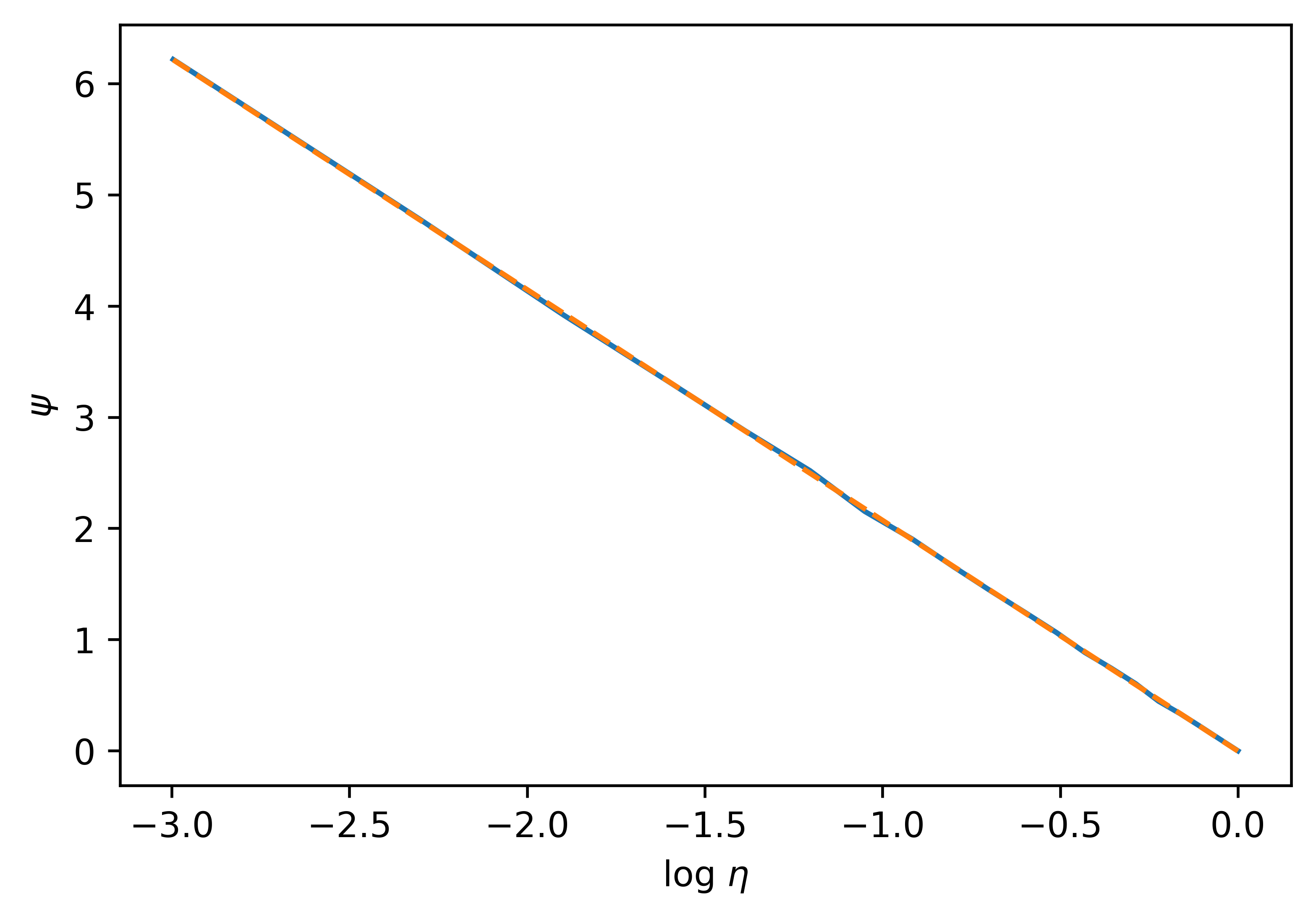
(b)

Figure 6: Evidence for the functional forms of the near-optimal function $g(h)$ and the subsampling cost function $\psi$. The dashed orange line in Panel 6(a) plots $\log g(h)=a_{1}h+b_{1}$ and the blue line plots the empirically observed $\log g(h)$ versus $h$. The dashed orange line in Panel 6(b) plots $\psi(\eta)=a_{2}\log\eta+b_{2}$ and the blue line plots the empirically observed $\psi(\eta)$ versus $\eta$.

16 Parameters used in Figure 1

Time Horizon	Method	$f$	$h$
T=1000	ss-LRB-10	45	1
	ss-LRB-20	70	1
	ss-LRB-30	100	0.9
	ss-LRB-40	100	0.9
	ss-LRB-50	100	0.9
	ss-LRB-60	100	1
	LRB	225	1
T=2000	ss-LRB-10	45	1.1
	ss-LRB-20	100	0.9
	ss-LRB-30	150	1
	ss-LRB-40	150	0.9
	ss-LRB-50	150	1
	ss-LRB-60	250	0.8
	LRB	225	1

References

- Abbasi-Yadkori et al. (2011) Abbasi-Yadkori, Yasin, Dávid Pál, Csaba Szepesvári. 2011. Improved algorithms for linear stochastic bandits. J. Shawe-Taylor, R. Zemel, P. Bartlett, F. Pereira, K. Q. Weinberger, eds., Advances in Neural Information Processing Systems, vol. 24. Curran Associates, Inc.
- Adams and Yellen (1976) Adams, William James, Janet L Yellen. 1976. Commodity bundling and the burden of monopoly. The quarterly journal of economics 475–498.
- Agarwal et al. (2021) Agarwal, Anish, Munther Dahleh, Devavrat Shah, Dennis Shen. 2021. Causal matrix completion. arXiv preprint arXiv:2109.15154 .
- Agrawal and Devanur (2014) Agrawal, Shipra, Nikhil R Devanur. 2014. Bandits with concave rewards and convex knapsacks. Proceedings of the fifteenth ACM conference on Economics and computation. 989–1006.
- Agrawal and Goyal (2012) Agrawal, Shipra, Navin Goyal. 2012. Analysis of thompson sampling for the multi-armed bandit problem. Conference on learning theory. 39–1.
- Allouah et al. (2021) Allouah, Amine, Achraf Bahamou, Omar Besbes. 2021. Optimal Pricing with a Single Point. arXiv e-prints arXiv:2103.05611.
- Aswad (2019) Aswad, Jem. 2019. Music streaming soared from 7% to 80% of u.s. market in the 2010s, riaa stats show.
- Athey et al. (2021) Athey, Susan, Mohsen Bayati, Nikolay Doudchenko, Guido Imbens, Khashayar Khosravi. 2021. Matrix completion methods for causal panel data models. Journal of the American Statistical Association 116(536) 1716–1730.
- Audibert et al. (2007) Audibert, Jean-Yves, Rémi Munos, Csaba Szepesvári. 2007. Tuning bandit algorithms in stochastic environments. International conference on algorithmic learning theory. Springer, 150–165.
- Auer et al. (2002a) Auer, Peter, Nicolo Cesa-Bianchi, Paul Fischer. 2002a. Finite-time analysis of the multiarmed bandit problem. Machine learning 47(2) 235–256.
- Auer et al. (2002b) Auer, Peter, Nicolo Cesa-Bianchi, Yoav Freund, Robert E Schapire. 2002b. The nonstochastic multiarmed bandit problem. SIAM journal on computing 32(1) 48–77.
- Bajari et al. (2021) Bajari, Patrick, Brian Burdick, Guido W Imbens, Lorenzo Masoero, James McQueen, Thomas Richardson, Ido M Rosen. 2021. Multiple randomization designs. arXiv preprint arXiv:2112.13495 .
- Banerjee et al. (2022) Banerjee, Siddhartha, Sean R Sinclair, Milind Tambe, Lily Xu, Christina Lee Yu. 2022. Artificial replay: A meta-algorithm for harnessing historical data in bandits. arXiv preprint arXiv:2210.00025 .
- Bastani and Bayati (2020) Bastani, Hamsa, Mohsen Bayati. 2020. Online decision making with high-dimensional covariates. Operations Research 68(1) 276–294.
- Bastani et al. (2022) Bastani, Hamsa, Pavithra Harsha, Georgia Perakis, Divya Singhvi. 2022. Learning personalized product recommendations with customer disengagement. Manufacturing & Service Operations Management 24(4) 2010–2028.
- Bayati et al. (2020) Bayati, Mohsen, Nima Hamidi, Ramesh Johari, Khashayar Khosravi. 2020. Unreasonable effectiveness of greedy algorithms in multi-armed bandit with many arms. Advances in Neural Information Processing Systems 33 1713–1723.
- Berry et al. (1997) Berry, Donald A, Robert W Chen, Alan Zame, David C Heath, Larry A Shepp. 1997. Bandit problems with infinitely many arms. The Annals of Statistics 2103–2116.
- Besbes and Mouchtaki (2021) Besbes, Omar, Omar Mouchtaki. 2021. How big should your data really be? data-driven newsvendor and the transient of learning. arXiv preprint arXiv:2107.02742 .
- Bhargava (2021) Bhargava, Hemant K. 2021. The creator economy: Managing ecosystem supply, revenue sharing, and platform design. Management Science .
- Bonald and Proutiere (2013) Bonald, Thomas, Alexandre Proutiere. 2013. Two-target algorithms for infinite-armed bandits with bernoulli rewards. Advances in Neural Information Processing Systems. 2184–2192.
- Brooks et al. (2011) Brooks, Steve, Andrew Gelman, Galin Jones, Xiao-Li Meng. 2011. Handbook of markov chain monte carlo. CRC press.
- Candes and Recht (2009) Candes, Emmanuel, Benjamin Recht. 2009. Exact matrix completion via convex optimization. Communications of the ACM 55(6) 111–119.
- Carpentier and Valko (2015) Carpentier, Alexandra, Michal Valko. 2015. Simple regret for infinitely many armed bandits. International Conference on Machine Learning. 1133–1141.
- Chaudhuri and Kalyanakrishnan (2018) Chaudhuri, Arghya Roy, Shivaram Kalyanakrishnan. 2018. Quantile-regret minimisation in infinitely many-armed bandits. UAI. 425–434.
- Chen et al. (2020) Chen, Y., Y. Chi, J. Fan, C. Ma, Y. Yan. 2020. Noisy matrix completion: Understanding statistical guarantees for convex relaxation via nonconvex optimization. SIAM Journal on Optimization 30(4) 3098–3121.
- Chu et al. (2011) Chu, Wei, Lihong Li, Lev Reyzin, Robert Schapire. 2011. Contextual bandits with linear payoff functions. Proceedings of the Fourteenth International Conference on Artificial Intelligence and Statistics. 208–214.
- Dani et al. (2008) Dani, Varsha, Thomas P Hayes, Sham M Kakade. 2008. Stochastic linear optimization under bandit feedback. Conference on Learning Theory .
- Davenport and Romberg (2016) Davenport, M. A., J. Romberg. 2016. An overview of low-rank matrix recovery from incomplete observations. IEEE Journal of Selected Topics in Signal Processing 10(4) 608–622. 10.1109/JSTSP.2016.2539100.
- Farias et al. (2021) Farias, Vivek F, Andrew A Li, Tianyi Peng. 2021. Uncertainty quantification for low-rank matrix completion with heterogeneous and sub-exponential noise. arXiv preprint arXiv:2110.12046 .
- Filippi et al. (2010) Filippi, Sarah, Olivier Cappe, Aurélien Garivier, Csaba Szepesvári. 2010. Parametric bandits: The generalized linear case. Advances in Neural Information Processing Systems. 586–594.
- Gabillon et al. (2012) Gabillon, Victor, Mohammad Ghavamzadeh, Alessandro Lazaric. 2012. Best arm identification: A unified approach to fixed budget and fixed confidence. Advances in Neural Information Processing Systems 25.
- Geng et al. (2020) Geng, Tong, Xiliang Lin, Harikesh S Nair. 2020. Online evaluation of audiences for targeted advertising via bandit experiments. Proceedings of the AAAI Conference on Artificial Intelligence, vol. 34. 13273–13279.
- Goldenshluger and Zeevi (2013) Goldenshluger, Alexander, Assaf Zeevi. 2013. A linear response bandit problem. Stochastic Systems 3(1) 230–261.
- Gopalan et al. (2014) Gopalan, Aditya, Shie Mannor, Yishay Mansour. 2014. Thompson sampling for complex online problems. International Conference on Machine Learning. 100–108.
- Gross (2011) Gross, David. 2011. Recovering low-rank matrices from few coefficients in any basis. IEEE Trans. Information Theory 57(3) 1548–1566.
- Gupta and Kallus (2022) Gupta, Vishal, Nathan Kallus. 2022. Data Pooling in Stochastic Optimization. Management Science 68(3) 1595–1615. 10.1287/mnsc.2020.3933. URL http://pubsonline.informs.org/doi/10.1287/mnsc.2020.3933.
- Gupta and Rusmevichientong (2021) Gupta, Vishal, Paat Rusmevichientong. 2021. Small-data, large-scale linear optimization with uncertain objectives. Management Science 67(1) 220–241.
- Hamidi and Bayati (2019) Hamidi, Nima, Mohsen Bayati. 2019. On low-rank trace regression under general sampling distribution. arXiv preprint arXiv:1904.08576 URL https://arxiv.org/pdf/1904.08576.pdf.
- Hamidi et al. (2019) Hamidi, Nima, Mohsen Bayati, Kapil Gupta. 2019. Personalizing many decisions with high-dimensional covariates. Advances in Neural Information Processing Systems. 11469–11480.
- Hao et al. (2020) Hao, Botao, Jie Zhou, Zheng Wen, Will Wei Sun. 2020. Low-rank tensor bandits. arXiv preprint arXiv:2007.15788 .
- Hastie et al. (2015) Hastie, Trevor, Robert Tibshirani, Martin Wainwright. 2015. Statistical Learning with Sparsity: The Lasso and Generalizations. Taylor & Francis, 2015.
- Johari et al. (2022) Johari, Ramesh, Hannah Li, Inessa Liskovich, Gabriel Y Weintraub. 2022. Experimental design in two-sided platforms: An analysis of bias. Management Science .
- Jun et al. (2019) Jun, Kwang-Sung, Rebecca Willett, Stephen Wright, Robert Nowak. 2019. Bilinear bandits with low-rank structure. International Conference on Machine Learning. PMLR, 3163–3172.
- Kaelbling (1993) Kaelbling, Leslie Pack. 1993. Learning in embedded systems. MIT press.
- Kallus and Udell (2020) Kallus, Nathan, Madeleine Udell. 2020. Dynamic assortment personalization in high dimensions. Operations Research 68(4) 1020–1037.
- Katariya et al. (2017) Katariya, Sumeet, Branislav Kveton, Csaba Szepesvari, Claire Vernade, Zheng Wen. 2017. Stochastic rank-1 bandits. Artificial Intelligence and Statistics. PMLR, 392–401.
- Katehakis and Robbins (1995) Katehakis, Michael N, Herbert Robbins. 1995. Sequential choice from several populations. Proceedings of the National Academy of Sciences of the United States of America 92(19) 8584.
- Keshavan et al. (2010) Keshavan, Raghunandan H, Andrea Montanari, Sewoong Oh. 2010. Matrix completion from a few entries. IEEE Trans. Informs. Theory 56 2980–2998.
- Keskin et al. (2020) Keskin, N Bora, Yuexing Li, Nur Sunar. 2020. Data-driven clustering and feature-based retail electricity pricing with smart meters. Available at SSRN 3686518 .
- Klopp (2014) Klopp, Olga. 2014. Noisy low-rank matrix completion with general sampling distribution. Bernoulli 20(1) 282–303.
- Kveton et al. (2017) Kveton, Branislav, Csaba Szepesvári, Anup Rao, Zheng Wen, Yasin Abbasi-Yadkori, S. Muthukrishnan. 2017. Stochastic low-rank bandits. CoRR abs/1712.04644.
- Kveton et al. (2020) Kveton, Branislav, Manzil Zaheer, Csaba Szepesvari, Lihong Li, Mohammad Ghavamzadeh, Craig Boutilier. 2020. Randomized exploration in generalized linear bandits. International Conference on Artificial Intelligence and Statistics. 2066–2076.
- Lai (1987) Lai, Tze Leung. 1987. Adaptive treatment allocation and the multi-armed bandit problem. The Annals of Statistics 1091–1114.
- Lattimore and Szepesvári (2020) Lattimore, Tor, Csaba Szepesvári. 2020. Bandit algorithms. Cambridge University Press.
- Li et al. (2010) Li, Lihong, Wei Chu, John Langford, Robert E Schapire. 2010. A contextual-bandit approach to personalized news article recommendation. Proceedings of the 19th international conference on World wide web. 661–670.
- Li et al. (2017) Li, Lihong, Yu Lu, Dengyong Zhou. 2017. Provably optimal algorithms for generalized linear contextual bandits. Proceedings of the 34th International Conference on Machine Learning-Volume 70. JMLR.org, 2071–2080.
- Lika et al. (2014) Lika, Blerina, Kostas Kolomvatsos, Stathes Hadjiefthymiades. 2014. Facing the cold start problem in recommender systems. Expert Systems with Applications 41(4) 2065–2073.
- Lops et al. (2011) Lops, Pasquale, Marco de Gemmis, Giovanni Semeraro. 2011. Content-based recommender systems: State of the art and trends. Recommender systems handbook 73–105.
- Lu (2019) Lu, Shaw. 2019. Beyond a-b testing: Multi-armed bandit experiments.
- Lu et al. (2018) Lu, Xiuyuan, Zheng Wen, Branislav Kveton. 2018. Efficient online recommendation via low-rank ensemble sampling. Proceedings of the 12th ACM Conference on Recommender Systems. 460–464.
- Lu et al. (2020) Lu, Y., A. Meisami, A. Tewari. 2020. Low-rank generalized linear bandit problems.
- McAfee et al. (1989) McAfee, R Preston, John McMillan, Michael D Whinston. 1989. Multiproduct monopoly, commodity bundling, and correlation of values. The Quarterly Journal of Economics 104(2) 371–383.
- Mersereau et al. (2009) Mersereau, Adam J, Paat Rusmevichientong, John N Tsitsiklis. 2009. A structured multiarmed bandit problem and the greedy policy. IEEE Transactions on Automatic Control 54(12) 2787–2802.
- Miao et al. (2019) Miao, Sentao, Xi Chen, Xiuli Chao, Jiaxi Liu, Yidong Zhang. 2019. Context-based dynamic pricing with online clustering. arXiv preprint arXiv:1902.06199 .
- Nakamura (2015) Nakamura, Atsuyoshi. 2015. A ucb-like strategy of collaborative filtering. Asian Conference on Machine Learning. PMLR, 315–329.
- Negahban and Wainwright (2012) Negahban, Sahand, Martin J Wainwright. 2012. Restricted strong convexity and weighted matrix completion: Optimal bounds with noise. Journal of Machine Learning Research 13(May) 1665–1697.
- Rohde et al. (2011) Rohde, Angelika, Alexandre B Tsybakov, et al. 2011. Estimation of high-dimensional low-rank matrices. The Annals of Statistics 39(2) 887–930.
- Rusmevichientong and Tsitsiklis (2010) Rusmevichientong, Paat, John N Tsitsiklis. 2010. Linearly parameterized bandits. Mathematics of Operations Research 35(2) 395–411.
- Russo (2016) Russo, Daniel. 2016. Simple bayesian algorithms for best arm identification. Conference on Learning Theory. PMLR, 1417–1418.
- Russo et al. (2017) Russo, Daniel, Benjamin Van Roy, Abbas Kazerouni, Ian Osband, Zheng Wen. 2017. A tutorial on thompson sampling. arXiv preprint arXiv:1707.02038 .
- Sam et al. (2022) Sam, Tyler, Yudong Chen, Christina Lee Yu. 2022. Overcoming the long horizon barrier for sample-efficient reinforcement learning with latent low-rank structure. arXiv preprint arXiv:2206.03569 .
- Schmalensee (1984) Schmalensee, Richard. 1984. Gaussian demand and commodity bundling. Journal of business S211–S230.
- Stigler (1963) Stigler, George J. 1963. United states v. loew’s inc.: A note on block-booking. The Supreme Court Review 1963 152–157.
- Thompson (1933) Thompson, William R. 1933. On the likelihood that one unknown probability exceeds another in view of the evidence of two samples. Biometrika 25(3/4) 285–294.
- Trinh et al. (2020) Trinh, Cindy, Emilie Kaufmann, Claire Vernade, Richard Combes. 2020. Solving bernoulli rank-one bandits with unimodal thompson sampling. Algorithmic Learning Theory. PMLR, 862–889.
- Volkovs et al. (2017) Volkovs, Maksims, Guangwei Yu, Tomi Poutanen. 2017. Dropoutnet: Addressing cold start in recommender systems. Advances in neural information processing systems 30.
- Wang et al. (2009) Wang, Yizao, Jean yves Audibert, Rémi Munos. 2009. Algorithms for infinitely many-armed bandits. D. Koller, D. Schuurmans, Y. Bengio, L. Bottou, eds., Advances in Neural Information Processing Systems 21. 1729–1736.
- Xu and Bastani (2021) Xu, Kan, Hamsa Bastani. 2021. Learning Across Bandits in High Dimension via Robust Statistics. Preprint.
- Ye et al. (2020) Ye, Zikun, Dennis Zhang, Heng Zhang, Renyu Philip Zhang, Xin Chen, Zhiwei Xu. 2020. Cold start to improve market thickness on online advertising platforms: Data-driven algorithms and field experiments. Available at SSRN 3702786 .
- Zhang et al. (2020) Zhang, Dennis, Ming Hu, Xiaofei Liu, Yuxiang Wu, Yong Li. 2020. Netease cloud music data .
- Zhang et al. (2014) Zhang, Mi, Jie Tang, Xuchen Zhang, Xiangyang Xue. 2014. Addressing cold start in recommender systems: A semi-supervised co-training algorithm. Proceedings of the 37th international ACM SIGIR conference on Research & development in information retrieval. 73–82.
- Zhu et al. (2022) Zhu, Ziwei, Xudong Li, Mengdi Wang, Anru Zhang. 2022. Learning markov models via low-rank optimization. Operations Research 70(4) 2384–2398.