Phase space representation of sound field in the Lake Kinneret

Abstract

The paper presents the analysis of pulsed sound fields recorded by a vertical array in the Lake Kinneret (Israel). The transition from the traditional representation of the complex amplitude of the received field as a function of depth and time to a function representing the field distribution in the phase space ‘depth - angle - time’ is considered. Due to the absence of multipath and problems with caustics, the sound field distribution in phase space is less sensitive to environmental disturbances and therefore more predictable than in configuration space. The transition is carried out using the coherent state expansion developed in the quantum theory. The found distribution of the field intensity in the phase space agrees with the calculation performed with an idealized environmental model. It is shown that this distribution can be taken as the input for solving the problem of source localization. The results of data processing demonstrate the possibility of using the coherent state expansion for isolating the field component formed by a given beam of rays.

1 Introduction

A characteristic feature of sound propagation in underwater waveguides is multipath [1, 2]. The field at the observation point usually represents a superposition of signals coming along different paths and therefore crossing different random inhomogeneities that are not taken into account in the available environmental model. As a result, the calculation of the complex amplitudes of these signals often turns out to be insufficiently accurate for theoretical prediction of the total field. This problem, which significantly complicates the solution of almost all problems of underwater acoustics, (source localization, underwater communication, remote sensing, etc.) is referred to as the uncertain environment [3, 4].

The present paper considers the approach introduced in Refs. [5, 6] for analyzing the sound field under condition of uncertain environment. This approach is based on the transition from the traditional description of the complex amplitude of the tonal field in the vertical section of the waveguide as a function of the depth $z$ to the amplitude distribution in the phase plane ‘depth - grazing angle’. This transition is carried out using the coherent state expansion developed in quantum mechanics [7, 8, 9]. The distributions of the amplitude and, especially, the intensity (squared amplitude) of the sound field in the phase space, represented in this example by the phase plane, turn out to be less sensitive to the medium perturbation than their distributions in the configuration space, represented by the $z$ axis. The reason is that there is no multipath in phase space: no more than one ray trajectory comes to any point in this space [10]. Similarly, when analyzing a field excited by a pulsed source, we can pass from the distribution of the field amplitude in the 2D phase plane ‘depth - time’ to its distribution in the 3D phase space ‘depth – angle – time’.

The function expressing the complex field amplitude dependence on the phase space coordinates is called the phase space representation of the sound field. Similar representations of wave fields are used in optics [9, 11].

Since the field amplitude distribution in the phase space, as noted above, is more stable with respect to the medium perturbation than the amplitude distribution in the configuration space, the transition to the phase space representation can reduce the requirements for the accuracy of environmental model when solving inverse problems. In Refs. [6, 12] this is demonstrated by the example of solving the problem of source localization in a waveguide.

In the present paper we examine the phase space representation of a pulsed sound field from a point source recorded in the Lake Kinneret (Israel) by a vertical receiving array. The measurements were taken in 2019 and 2021. The main attention is paid to the comparison of the received field intensity distribution in the phase space ‘depth - angle - time’ with the results of numerical simulation.

The paper is organized as follows. Section 2 describes the experiments and the data obtained. Two idealized models of range-independent waveguide used for numerical simulation are also presented here. The main provisions of the theory used in the construction of the phase space representation are outlined in Sec. 3. The results of data processing are presented in Sec. 4. In this section, the calculated and measured distributions of the field intensity in the phase space ’depth - angle - time’ are compared. This section also demonstrates the possibility of using these distributions as input to solve the source localization problem. The results of the work are summarized in Sec. 5.

2 Experimental data and environmental model

Subtropical Lake Kinneret (the Sea of Galilee) is an example of a fresh water reservoir, with changing stratification: approximately constant temperature 15-16^∘ C over all the depth in the Winter and reaching 30^∘ C in upper layer in the Summer. Approximate size is 12 x 22 km, maximal depth of the lake is 40 m, depth of thermocline 10-20 m.

Acoustic measurements were carried out in 2019 and 2021 in the central part of the lake where the bottom is almost flat. The signals were recorded using a receiving vertical array of 10 hydrophones, and the radiation was performed by a source lowered from a drifting vessel. The table shows the distances from which the signals were recorded.

Table 1: Observation distances

Year	Distances
2019	340 m, 380 m
2021	415 m, 905 m, 1445 m

In 2019, at each of the indicated distances, a source located at a depth of 10 m emitted chirp pulses with a duration of 1 s in the frequency band from 300 to 3500 Hz. The receiving hydrophones covered the depth interval from 10 to 37 m with a step of 3 m. The sound speed profile measured near the receiving array is shown on the left side of Fig. 1. The dots show the depths of the receiving hydrophones.

In 2021, at the distances indicated in the table, the source was located at a depth of 7 m and emitted chirp pulses with a duration of 5 s in the frequency band from 200 Hz to 10 kHz. The sound speed profile and hydrophone depths are shown on the right side of Fig. 1. The hydrophones covered the depth interval from 7 to 34 m with a step of 3 m.

Figure 1: Sound speed profiles and hydrophone positions in 2019 (left panel) and 2021 (right panel).

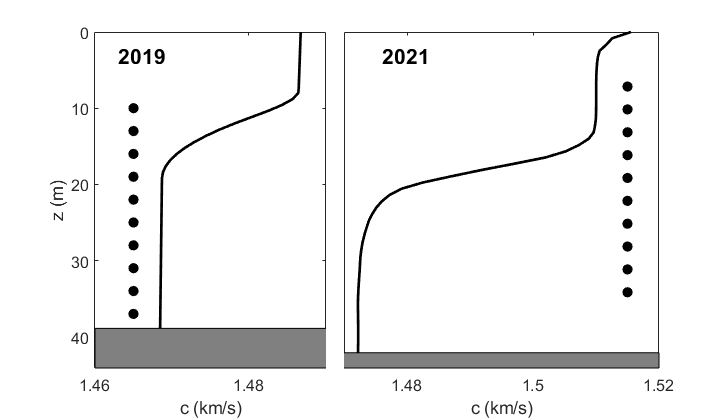
When simulating the measured acoustic fields, we used range-independent waveguide models with sound speed profiles from the left and right sides of Fig. 1. Due to the difference in water surface levels, the waveguide depths in 2019 and 2021 were slightly different (this is shown in Fig. 1). In simulation, they were taken equal to 38.9 m and 42.1 m, respectively.

The bottom structure of Lake Kinneret is complex. In central area, the sediment is composed mainly of clays and carbonate. The presence of gas (methane) bubbles in the upper sediment was found earlier and confirmed by many direct measurements. Both concentration of bubbles (less than 0.5 - 1%) and thickness of gassy layer (less than 50 - 70 cm) change in dependence on place and season [13]. For our purpose in this paper, we can use a simplified geoacoustic model representing a liquid homogeneous half-space.

In the present paper, our objective is to analyze the field components formed by narrow beams of rays whose grazing angles near the bottom do not exceed $42^{\circ}$. In Lake Kinneret, due to the high concentration of gas bubbles in sediments, waves with such grazing angles are almost completely reflected from the bottom. In both our waveguide models, the bottom is represented by a liquid half-space with a sound speed of 2 km/s and a density of 1400 kg/m³. Although these environmental models are obviously inexact, they correctly reflect the fact that waves with the indicated grazing angles are completely reflected from the lower boundary of the waveguide. In this case the reflection coefficients for all rays of a narrow beam are approximately equal to $V=\exp(i\phi)$, where $\phi$ is the angle whose value cannot be predicted within the framework of our model. We assume that, despite the inaccuracy of the bottom model, the desired field components can be approximately calculated up to unknown phase factors $V^{N}$, where $N$ is the number of beam reflections from the bottom. Below we will see that this is sufficient for the evaluation of the sound field intensity in the phase space.

The sound field of a point source in a range-independent waveguide is a function of distance $r$, depth $z$, and time $t$. The $z$ axis is directed vertically downwards and the water surface is at the horizon $z=0$. At the observation distance, that is, for a fixed $r$, we represent the complex field amplitude as the Fourier integral

$$v\left(z,t\right)=\int df~{}u\left(z,f\right)e^{-2\pi ift}.$$ (1)

The calculation of the Fourier components $u\left(z,f\right)$ at frequencies $f$ in the band of the emitted signal was performed by the normal mode method [1, 15].

As mentioned above, the sound field $v\left(z,t\right)$ was measured only at 10 horizons $z_{n}$, $n=1,\ldots,10$. Accordingly, the values of functions $u\left(z,f\right)$ are known only at these depths.Using these data, one can approximately estimate the amplitudes of the propagating modes [14] and then reconstruct functions $u\left(z,f\right)$ over the entire vertical section of the waveguide. Let us use the representation of the function $u\left(z,f\right)$ as a superposition of eigenfunctions $\varphi_{m}\left(z,f\right)$ of the Sturm-Liouville problem for a model waveguide

$$u\left(z,f\right)=\sum_{m=1}^{M\left(f\right)}b_{m}\left(f\right)\varphi_{m}\left(z,f\right),$$ (2)

where $M\left(f\right)$ is the number of propagating modes. Substituting the values of functions $u\left(z,f\right)$ and $\varphi_{m}\left(z,f\right)$ at 10 points $z_{n}$ into this equality, we get (at each frequency $f$) a system of 10 equations for the $M\left(f\right)$ unknowns $b_{m}\left(f\right)$. At all frequencies in the band of the emitted signal, this system is underdetermined. Its approximate solution can be found using the pseudoinverse matrix. Substituting the found values $b_{m}\left(f\right)$ into (2) gives an expression for calculating the field at an arbitrary depth. Due to the fact that there are only ten receiving hydrophones and the distance between neighboring hydrophones (3 m) is relatively large, the obtained solution of the inverse problem has an acceptable accuracy only at low frequencies in the $300$ Hz $<f<900$ Hz band.

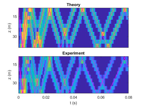
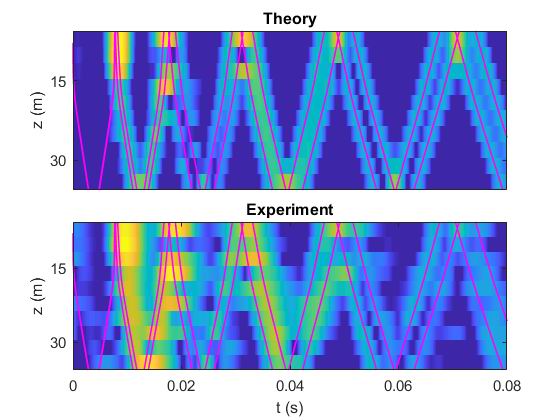
To eliminate the contributions of higher frequencies, the recorded signals were bandpass filtered with the spectral weight $\exp\left(-\pi\left(f-f_{c}\right)^{2}/\Delta_{f}^{2}\right)$, where $f_{c}$ = 600 Hz and $\Delta_{f}$ = 300 Hz. The amplitudes of bandpassed signals at the horizons $z_{n}$, received from distances of 380 m and 905 m, are shown in Figs. 2 and 3, respectively. Here and in what follows, for brevity, we indicate only the distance to the source, omitting the year of measurements (see Table I). The upper and lower panels of the figures show the results of theoretical calculations and the measurement data, respectively. In each plot, the magenta broken lines represent the timefront depicting ray arrivals in the $\left(t,z\right)$ plane. The timefronts were calculated using the corresponding waveguide models. The figures show the initial sections of the recorded signals with a duration of 0.08 s. Further, when comparing theory and experiment, we analyze fragments of the received fields in this time interval.

Figure 2: Signal amplitudes $\left|v\left(z,t\right)\right|$ on receiving array elements recorded from a distance of 380 m. Top: numerical simulation. Bottom: measurement data. The magenta broken lines represent the time front.

Figure 3: The same as in Fig. 2, but for signals received from 905 m.

3 Theory

In this section, we consider a theoretical description of the field excited by a point source in a range-independent waveguide with a sound speed profile $c\left(z\right)$ and a refractive index $n\left(z\right)=c_{0}/c\left(z\right)$, where $c_{0}$ is the reference sound speed.

3.1 Ray paths in the phase space

The phase space appears in the Hamiltonian formulation of classical mechanics and geometrical optics [10, 11, 16]. Within the framework of this formalism, the ray trajectory at distance $r$ is determined by its depth $z$ and momentum $p=n\left(z\right)\sin\chi$, where $\chi$ is the grazing angle at the point $\left(r,z\right)$. The ray equations take the form of the Hamilton equations $dz/dr=-\partial H/\partial p$, $dp/dr=-\partial H/\partial z$, where $H=-\sqrt{n^{2}\left(z\right)-p^{2}}$ is the Hamiltonian. The functions $p\left(r,p_{0},z_{0}\right)$ and $z\left(r,p_{0},z_{0}\right)$ representing solutions of these equations with initial conditions $p\left(0\right)=p_{0}$ and $z\left(0\right)=z_{0}$, describe the ray trajectory.

The ray travel time $t\left(r,p_{0},z_{0}\right)$, i.e. the travel time of sound along the ray path, is analogous to the action integral or the Hamilton’s principal function in mechanics. This function is given by the integral along the ray path $c_{0}t=\int\left(pdz-Hdt\right)$ [11, 16].

In the case of a point source, all rays at $\ r=0$ escape from the same depth $z_{s}$ with different launch angles $\chi_{0}$ and, accordingly, with different starting momenta $p_{0}=n\left(z_{s}\right)\sin\chi_{0}$. The arrival of a ray at a given observation distance $r>0$ is represented by a point in the phase space $\left(z,p,t\right)$. The set of such points forms a curve, which we call the ray line in the 3D phase space $\left(z,p,t\right)$. It is parametrically determined by the equations: $p=p\left(r,p_{0},z_{s}\right)$, $z=z\left(r,p_{0},z_{s}\right)$ and $t=t\left(r,p_{0},z_{s}\right)$.

Choosing the reference sound speed $c_{0}$ = 1.5 km/s in waveguides with $c\left(z\right)$ profiles shown in Fig. 1, we get $n$ values close to one. For flat rays, the momentum $p$ is approximately equal to the grazing angle $\chi$. Therefore, the phase space $\left(z,p,t\right)$ can be called the ’depth – angle – time’ space.

Figure 4: Fragments of ray lines at a distance of 380 m in the time interval of 0.02$\div$0.07 s (upper panel) and at a distance of 905 m in the time interval of 0.03$\div$0.07 s (lower panel). The black circles $A$ (top panel) and $B$ (bottom panel) show the arrivals of rays that escape the source with launch angles $-30^{\circ}$ and $19.5^{\circ}$, respectively.

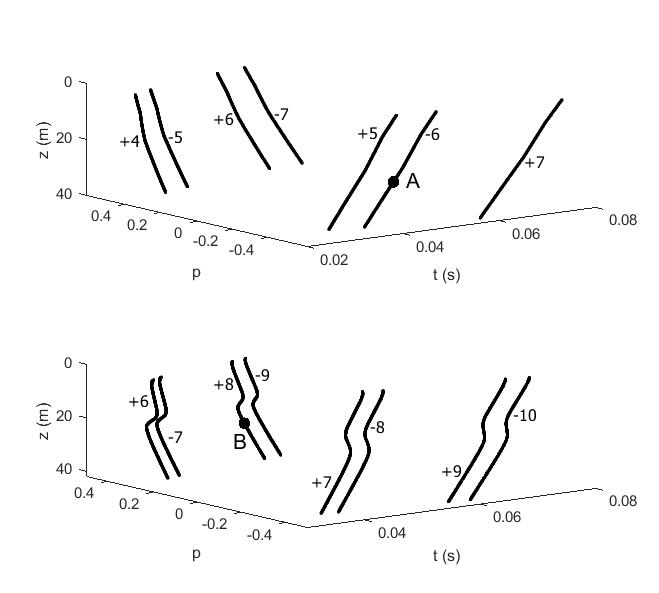
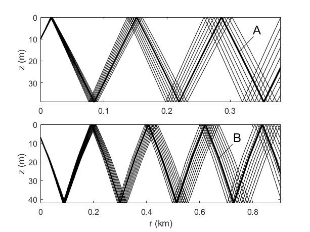
Figure 4 shows fragments of ray lines at distances of 380 m (upper panel) and 905 m (lower panel). The ray line consists of segments formed by trajectories with the same identifiers $\pm M$, where $\pm$ is the sign of launch angle (+ corresponds to the rays starting towards the bottom), and $M$ is the number of turning points. In our case, for almost all rays, the turning points are the points of reflection from the boundaries. In what follows, the segment depicting the arrivals of rays with the identifier $\pm M$ will be called, for brevity, the segment $\pm M$.

Note that for rays propagating without reflections from boundaries in a refracting waveguide, the ray line is continuous [5, 6, 12]. In our example, discontinuities arise due to the fact that when reflected from the boundary, the ray grazing angle, and hence its momentum, changes sign.

On each of the ray lines shown in Fig. 4, the arrival of one of the rays is marked with a black circle. On the top panel, this is ray $A$ which escaped the source at a launch angle of $-30^{\circ}$. Its identifier at the observation range is -6. The trajectory of this ray (bold line) and the trajectories of other rays forming segment -6 are shown at the top of Fig. 5.

On the bottom panel of Fig. 4, the black circle marks the arrival of ray $B$ whose launch angle is $19.5^{\circ}$. At a distance of 905 m, its identifier is +8. The beam of rays forming segment +8 is shown at the bottom of Fig. 5. The trajectory of ray $B$ is marked with a bold line.

Figure 5: Top panel. Ray trajectories forming segment -6 (thin lines) at 380 m. The bold line shows the trajectory of ray $A$. Bottom panel. Ray trajectories forming segment +8 (thin lines) at 905 m. The bold line shows the trajectory of ray $B$.

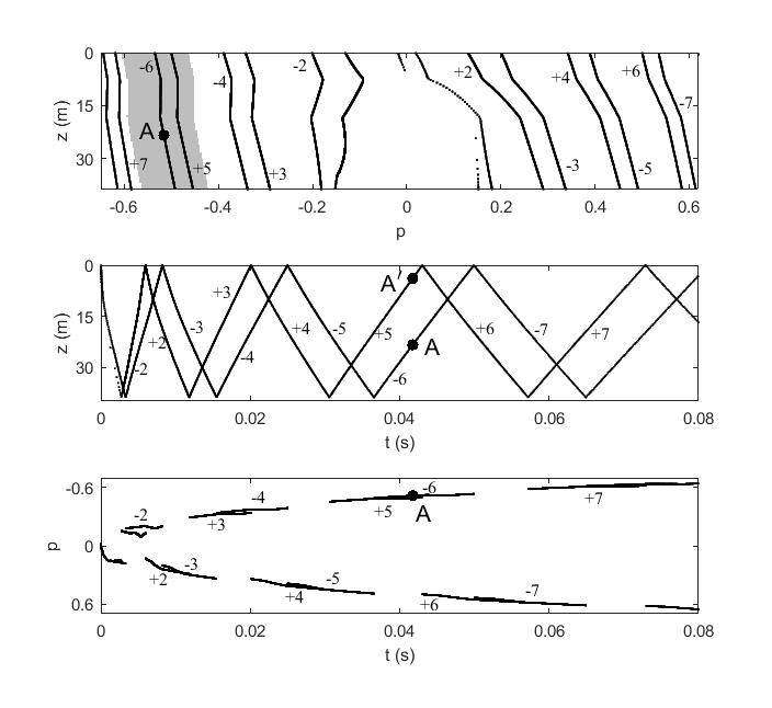
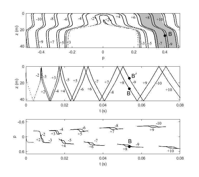
Figures 6 and 7 show the projections of the ray lines from Figs. 4 on the planes $\left(p,z\right)$ (top), $\left(t,z\right)$ (middle), and $\left(t,p\right)$ (bottom). Each segment of the ray line is represented by its projections onto the indicated planes. A corresponding identifier is indicated next to each projection. Projections onto the $\left(t,z\right)$ plane shown in the upper panels of Fig. 6 and 7 represent the timefronts shown by the magenta lines in Fig. 2 and 3, respectively. The arrival of ray $A$ in fig. 6 is shown with a black circle. In addition, in the middle panel of Fig. 6, the arrival of ray $A^{\prime}$ with the travel time equal to the travel time of ray $A$ is highlighted. Similarly, in Fig. 7, the arrivals of ray $B$ are highlighted. The middle panel also highlights the arrival of ray $B^{\prime}$ with the same travel time as that of ray $B$.

In the upper panels of Fig. 6 and 7, the areas representing the so-called fuzzy segments are shown in grey. They will be considered further in Sec. 3.3.

Figure 6: Projections of the ray line at a distance of 380 m (Fig. 4, top panel) on the planes $\left(p,z\right)$ (top), $\left(t,z\right)$ (middle), and $(t,p)$ (bottom). Near each segment, the corresponding identifier is indicated. The black circles on all panels highlight the arrival of ray $A$. The middle panel also highlights the arrival of ray $A^{\prime}$ with the same travel time as that of ray $A$.

Figure 7: The same as in fig. 6, but for a distance of 905 m. The arrivals of ray $B$ and ray $B^{\prime}$ whose travel time is the same as that of ray $B$ are marked with the black circles.

3.2 Coherent state expansion

The function $u\left(z,f\right)$ on the right side of (1) represents the depth dependence of the complex field amplitude at some fixed frequency $f$. For brevity, in this and the next section, the argument $f$ will be omitted. All our subsequent analysis is based on the transition from $u\left(z\right)$ to a function characterizing the distribution of the field amplitude in the phase plane ’depth – momentum (angle)’ $\left(z,p\right)$. The transition is carried out using the coherent state expansion [9].

The coherent state associated with the point $\mu=\left(z,p\right)$ of the phase plane is determined by the function

$$Y_{\mu}\left(z^{\prime}\right)=\frac{1}{\sqrt{\Delta_{z}}}\exp\left[ikp\left(z^{\prime}-z\right)-\frac{\pi\left(z^{\prime}-z\right)^{2}}{2\Delta_{z}^{2}}\right],$$ (3)

where $\Delta_{z}$ is the vertical scale, $k=2\pi f/c_{0}$ is the reference wavenumber. In quantum mechanics, (3) describes a state with the minimum uncertainty, that is, with the minimum product of the standard deviations of the position and momentum [17]. In acoustics (3) describes the vertical section of a wave beam with the smallest possible product of the beam width by the spread of the grazing angles of the waves forming it.

Although the coherent states are not orthogonal, they form a complete system of functions and an arbitrary function $u(z^{\prime})$ can be represented as an expansion [8, 9]

$$u\left(z^{\prime}\right)=\lambda^{-1}\int d\mu~{}a_{\mu}Y_{\mu}\left(z^{\prime}\right),$$ (4)

where

$$a_{\mu}=\int dz^{\prime}~{}u\left(z^{\prime}\right)Y_{\mu}^{\ast}\left(z^{\prime}\right),$$ (5)

superscript * means complex conjugate. In these relations, integration over $\mu$ goes over the entire phase plane, and integration over $z^{\prime}$ goes over the entire vertical axis.

The complex amplitude $a_{\mu}$ at the point $\mu=\left(z,p\right)$ represents the projection of the field in the vertical section of the waveguide onto the coherent state (3). It quantitatively characterizes the contribution of waves coming to depths close to $z$ at grazing angles close to $\arcsin p$. Thus, $a_{\mu}$ characterizes the distribution of the field amplitude in the phase plane ’depth – angle’. The squared amplitude $\left|a_{\mu}\right|^{2}$ in quantum theory is called the Husimi function [9]. In what follows we will call it the intensity of the coherent state.

The closeness of the coherent states associated with the points of the phase plane $\mu=\left(z,p\right)$ and $\mu_{1}=\left(z_{1},p_{1}\right)$ can be quantitatively characterized by their squared scalar product

$$\left|\int dz^{\prime}~{}Y_{\mu}\left(z^{\prime}\right)Y_{\mu_{1}}^{\ast}\left(z^{\prime}\right)\right|^{2}=e^{-\frac{1}{2}d\left(\mu,\mu_{1}\right)},$$ (6)

where

$$d\left(\mu,\mu_{1}\right)=\frac{\pi\left(z-z_{1}\right)^{2}}{\Delta_{z}^{2}}+\frac{\pi(p-p_{1})^{2}}{\Delta_{p}^{2}},$$ (7)

$\Delta_{p}=\lambda/(2\Delta_{z})$, $\lambda=2\pi/k$ is the wavelength. We will interpret the quantity $d\left(\mu,\mu_{1}\right)$ as a dimensionless distance between the points $\mu$ and $\mu_{1}$. The coherent states associated with these points will be considered close for $d<1$ and different for $d>1$. The distance from the point $\mu$ to a curve in the phase plane (for example, to the ray line or to its segment) is the distance from $\mu$ to the nearest point of the curve.

The complex amplitude $a_{\mu}$ is defined for any point $\mu$ of the phase plane. However, according to (5) – (7), the coherent state intensities $\left|a_{\mu}\right|^{2}$ take on maximum values near the points corresponding to ray arrivals. These points lie on the projection of the ray line on the plane $\left(z,p\right)$. We will call this projection a ray line in the phase plane. In mechanics and geometric optics, it is called the Lagrangian manifold [11]. Examples of such lines are presented in the upper panels of Figs. 6 and 7.

The main contribution to $u\left(z\right)$ comes from coherent states associated with points $\mu$ located at distances $d<1$ from the ray line. We call this part of the phase plane the fuzzy ray line. Its area is determined by the choice of the coherent state scales $\Delta_{z}$ and $\Delta_{p}$. Since they are related by the uncertainty relation $\Delta_{z}\Delta_{p}=\lambda/2$, then in fact we are talking about choosing one of these scales. Ref. [6] discusses the choice of $\Delta_{z}$ to minimize the area. It is clear that for $\Delta_{z}\rightarrow 0$ and $\Delta_{z}\rightarrow\infty$ the area increases indefinitely. The minimum corresponds to some finite $\Delta_{z}$, which is determined by the shape of the ray line. In Ref. [6] it is shown that this scale is proportional to $\lambda^{1/2}$.

3.3 Isolation of contribution from a given beam of rays to the total field

Let us take a particular segment of the ray line in the phase plane. In accordance with the above, the contribution to the total field of rays represented by this segment is expressed as a superposition of coherent states associated with the phase plane points located at distances $d<1$ from the segment. The area $\sigma$ formed by these points is called the fuzzy segment of the phase plane. Consider a field component

$$U\left(z^{\prime}\right)=\lambda^{-1}\int_{\sigma}d\mu~{}a_{\mu}Y_{\mu}\left(z^{\prime}\right),$$ (8)

where the integration is over the fuzzy segment $\sigma$. It is natural to interpret this component as a contribution to the total field of the beam of rays that form the selected segment. Using (4) and (5), this expression can be rewritten as [5]

$$U\left(z^{\prime}\right)=\int dz^{\prime\prime}~{}\Pi\left(z^{\prime},z^{\prime\prime}\right)u\left(z^{\prime\prime}\right),$$ (9)

where

$$\Pi\left(z^{\prime},z^{\prime\prime}\right)=\lambda^{-1}\int_{\sigma}d\mu~{}Y_{\mu}\left(z^{\prime}\right)Y_{\mu}^{\ast}\left(z^{\prime\prime}\right).$$ (10)

Thus, the isolation of the beam contribution to the total field is carried out using linear spatial filtering. By selecting the area $\sigma$ the filter is ’tuned’ to the required beam.

In this paper, we consider beams that (i) are formed by rays with the same identifier and (ii) cover the entire vertical section of the waveguide at the observation distance. Examples of such beams are shown in Fig. 5. However, the described procedure is applicable to any beam of rays. In the case of free space, when the field on the antenna is a fragment of a plane wave formed by a beam of parallel rays, the described procedure is reduced to the standard formation of an antenna lobe.

Isolation of the beam contribution by this method is possible only if the fuzzy segments of the phase plane corresponding to different beams do not overlap. This requirement can only be met at sufficiently high frequencies. In Sec. 2 it is noted that when processing experimental data, we can analyze signals only in the 600$\pm$300 Hz band. Gray areas in the upper panels of Fig. 6 and 7 represent fuzzy segments at 600 Hz, for -6 and +8 segments, respectively. In both cases, neighboring segments fall into the gray areas. This means that the selected fuzzy segments overlap with neighboring fuzzy segments, and when processing the tonal signals, the contributions of corresponding beams of rays cannot be resolved. However, we will see below that, when dealing with pulsed signals, the spatial resolution is supplemented by the temporal one, and the isolation of individual beams becomes possible.

3.4 Pulse signals

Using (4) and (5), we represent the complex amplitude $u\left(z,f\right)$ at each frequency $f$ as a superposition of coherent states. Then the coherent state amplitude $a_{\mu}$ becomes a function of $f$. When calculating this function, the scale $\Delta_{z}$ can be chosen different for different frequencies.

Let us introduce the function

$$a\left(z,p,t\right)=\int df~{}a_{\mu}\left(f\right)e^{-2\pi ift},$$ (11)

characterizing the distribution of the transient field amplitude in phase space ’depth –momentum (angle) – time’ $\left(z,p,t\right)$. For points of this space lying on a ray line, the function $a\left(z,p,t\right)$ can be interpreted as the complex amplitude of a sound pulse that comes to depth $z$ at grazing angle $\arcsin p$ at time $t$.

Further, when processing the experimental data, the main attention will be paid to the analysis of the coherent state intensity

$$J\left(z,p,t\right)=\left|a\left(z,p,t\right)\right|^{2}.$$ (12)

This function takes the largest values near the ray line, and decreases as it moves away from it.

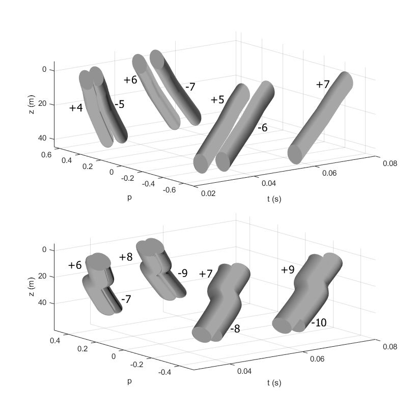
In Sec. 3.2, it is shown that in the case of a tonal sound field, the distribution of coherent states intensity $\left|a_{\mu}\right|^{2}$ is localized inside the fuzzy ray line in the phase plane. In 3D phase space $\left(z,p,t\right)$, we introduce a similar area, which will also be called a fuzzy ray line. We define its boundary as follows. The signal arrival times $t$ at the observation distance belong to a certain interval $t_{\min}<t<t_{\max}$. Let’s choose an arbitrary time $t_{\ast}$ from this interval and consider the plane $\left(z,p\right)$ formed by points of the phase space with $t=t_{\ast}$. This plane intersects the ray line at, generally speaking, several points. Timefronts in the middle panels of Figs. 6 and 7 show that in our waveguide model, for any $t_{\ast}$, there are two intersection points. Examples of such pairs are points A and A’ in Fig. 6 and points B and B’ in Fig. 7. Let $\mu_{\ast}=\left(z_{\ast},p_{\ast}\right)$ be one of the intersection points. As the boundary of the fuzzy ray line in the neighborhood of $\mu_{\ast}$, we take the ellipse formed by the points $\mu$ that are spaced from $\mu_{\ast}$ by the dimensionless distance $d\left(\mu,\mu_{\ast}\right)=1$. The dimensionless distance (7) depends on the frequency $f$, and when defining the boundary, we evaluate this distance for the center frequency of the analyzed signal. In our case, this is $f$ = 600 Hz. Figure 8 presents fragments of fuzzy ray lines at distances of 380 (top) and 905 m (bottom). The segments of the ray line shown in Fig. 4, here turned into tubes of finite thickness.

Figure 8: Fragments of fuzzy ray lines at distances of 380 (top) and 905 m (bottom). The corresponding identifier is indicated next to each fuzzy segment.

The procedure for isolating the ray beam contribution to the tonal field, described in Sec. 3.3, is naturally generalized to the case of a pulsed source. First, the procedure is used to isolate the beam contribution $U\left(z,f\right)$ from the component of the total field $u\left(z,f\right)$ at each frequency $f$ in the band of the emitted signal. Then the beam contribution to the total field $v\left(z,t\right)$ is synthesized via the Fourier transformation

$$V\left(z,t\right)=\int df~{}U\left(z,f\right)e^{-2\pi ift}.$$ (13)

Analytical relations, presented above, suggest, that the amplitude of the coherent state $a_{\mu}$ associated with a point $\mu=(z,p)$ in the phase space is determined mainly by the contributions of rays arriving in the depth interval $z\pm\Delta_{z}/2$. In the examples considered below, such rays have approximately the same bottom reflection coefficients $V$. As indicated in Sec. 2, in this paper we consider the field components that are completely reflected from the bottom and therefore $V=\exp(i\phi)$. Due to the inaccuracy of the bottom model, we cannot correctly calculate the coefficient $V$ and therefore the complex amplitude $a_{\mu}$ can be found only up to an unknown phase factor. However, the intensity $|a_{\mu}|^{2}$ is calculated correctly in this case. Moreover, we assume a weak dependence of the coefficient $V$ on the frequency (in the band of the emitted signal). Then the intensity of the pulsed field $J\left(z,p,t\right)$ is also correctly predicted. The validity of these assumptions is confirmed by the comparison of theory and experiment presented in the next section.

4 Data analysis

When processing experimental data, our attention was focused on calculating the distribution of the sound field intensity $J\left(z,p,t\right)$ in the 3D phase space $\left(z,p,t\right)$. The results of calculating these distributions for fields recorded at distances of 380 and 905 m are compared with theoretical predictions. Similar comparisons made for the other three distances look similarly and are therefore not presented here. This section also demonstrates that the obtained intensity distributions $J\left(z,p,t\right)$ can be used to estimate the distance to the source. This is done for the all five distances.

One of the reasons for the discrepancy between theory and experiment is the errors in the reconstruction of the field in the vertical section of the waveguide from the measurement data at only 10 horizons. To assess the influence of this factor, we present two variants of numerical simulation. The first of them is performed for a receiving array of a large number of elements (with an interelement distance small compared to the wavelength), which uniformly fill the entire vertical section of the waveguide. The second variant is based on the theoretical calculation of the sound field at ten points of the vertical section corresponding to the hydrophone depths. The field in the entire vertical section is reconstructed in exactly the same way as in the processing of experimental data. On the plots representing the results obtained by the first and second methods, it is indicated ’Theory, dense array’ and ’Theory, sparse array’, respectively.

In the coherent state expansion for all distances and all frequencies, the vertical scale $\Delta_{z}$ is equal to $10$ m.

4.1 Intensity distribution in phase space ($z,p,t$)

Let us consider the function $J\left(z,p,t\right)$ representing the intensity distribution of the field registered at a distance of 380 m. A fragment of the ray line in 3D phase space for this distance is shown in the upper panel of Fig. 4, and the projections of this line on the planes $\left(p,z\right)$, $\left(t,z\right)$, and $\left(t,p\right)$ are in Fig. 6. The point representing the arrival of ray $A$ has the coordinates $\left(z_{A},p_{A},t_{A}\right)$, where $z_{A}$ = 23.4 m, $p_{A}$ = -0.52, and $t_{A}=$0.4 s.

Figure 9 presents a section of the function $J\left(z,p,t\right)$ by the plane $t=t_{A}$. At points $A$ and $A^{\prime}$, shown by white circles, this plane is crossed by ray line segments -6 and +5, respectively. In the top panel of Fig. 9 we see that the points $A$ and $A^{\prime}$ are located near the local maxima of the intensity distribution in the plane $\left(p,z\right)$. Note that the point $A^{\prime}$ is located on the horizon 3.9 m, located outside the depth interval covered by the receiving array. Therefore, the field near $A^{\prime}$ is poorly reconstructed, and the corresponding local maximum of the intensity distribution is hardly noticeable on the middle and lower panels. Magenta ellipses in the upper panel are formed by points that are spaced from A and A’ by dimensionless distances $d=1$ (at a frequency of 600 Hz). These ellipses represent the intersections of the $t=t_{A}$ plane and the boundaries of the fuzzy segments corresponding to identifiers -6 and +5.

Figure 9: Cross section of the intensity distribution $J\left(z,p,t\right)$ at a distance of 380 m by the plane $t=t_{A}$. Top and middle panels: numerical simulations. Bottom panel: experiment. The white circles indicate the arrivals of rays A and A’ in the phase plane. Magenta ellipses in the upper panel show the boundaries of fuzzy segments +6 (around point A) and -5 (around point A’) in the plane $t=t_{A}$.

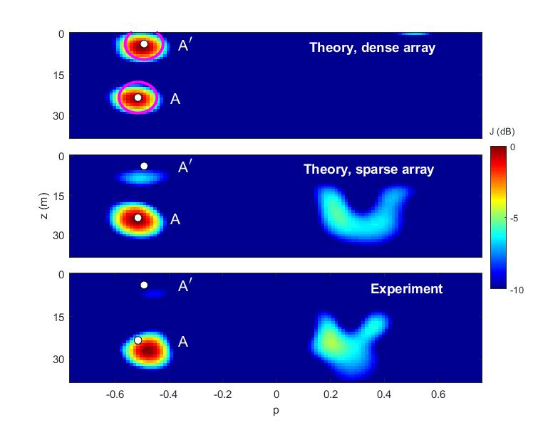
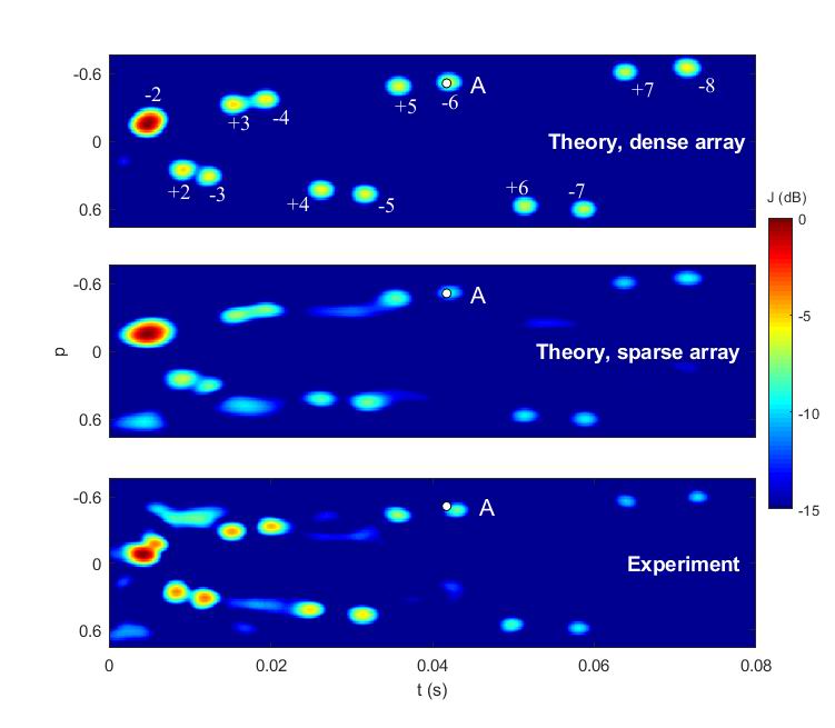
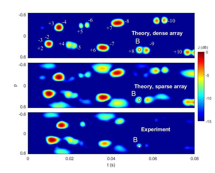
Figure 10 shows a section of the function $J\left(z,p,t\right)$ by the plane $z=z_{A}$. This plane intersects all segments of the ray line, and in the vicinity of each intersection point, an area of increased intensity is observed. The identifier of the corresponding segment is indicated next to each area of high intensity. Horizon $z_{A}$ is located within the depth interval covered by the receiving array. Therefore, the field in the vicinity of this point is reconstructed quite well, and the intensity peaks predicted by the theory are clearly distinguished on the all three panels.

Figure 10: Cross section of the intensity distribution $J\left(z,p,t\right)$ at a distance of 380 m by the plane $z=z_{A}$. Top and middle panels: numerical simulations. Bottom panel: experiment. The white circles indicate the arrival of ray $A$. In the upper panel, next to each local maximum, the identifier of the corresponding segment is indicated.

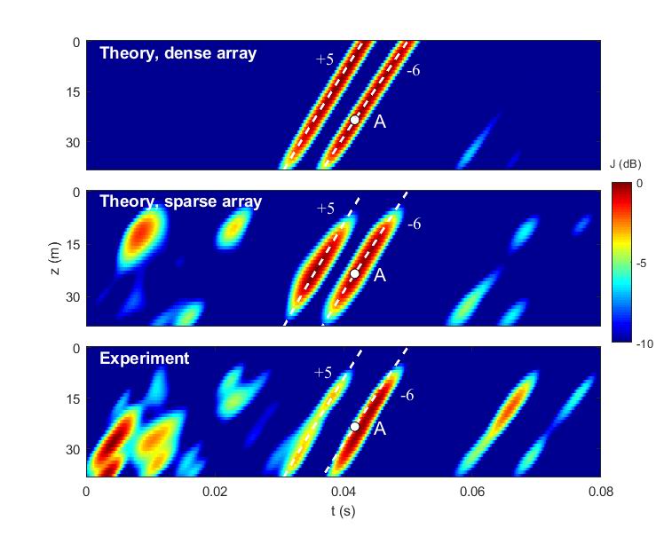
The section by the plane $p=p_{A}$ is shown in Fig. 11. This plane intersects the ray line segments -6 and +5. The projections of these segments onto the $\left(t,z\right)$ plane are shown as white dotted lines. The point of the intersection with segment -6, marked with a white circle, depicts the arrival of ray $A$. The rays forming segments -6 and +5 at the observation distance have momenta $p$ close to $p_{A}$. Therefore, in this particular example, the obtained intensity distribution in the time-depth plane $\left(t,z\right)$ practically coincides with the intensity distribution $\left|V\left(z,t\right)\right|^{2}$ at the output of the filter, determined by equations (9) and (13), and tuned to isolate a beam of rays with identifier -6. We have already noted (Sec. 3.3) that the fuzzy segment -6 shown in the top panel of Fig. 5 overlaps with segment +5. This means that when dealing with tonal field at a frequency of 600 Hz, the contributions of ray beams with identifiers +5 and -6 cannot be separated. In Fig. 10 we see that in the case of a pulsed source, the additional temporal resolution made it possible to isolate the contributions of these beams.

Figure 11: Cross section of the intensity distribution $J\left(z,p,t\right)$ at a distance of 380 m by the plane $p=p_{A}$. Top and middle panels: numerical simulations. Bottom panel: experiment. The white circle shows the arrival of ray $A$. The white dotted lines show the projections of segments +5 and -6.

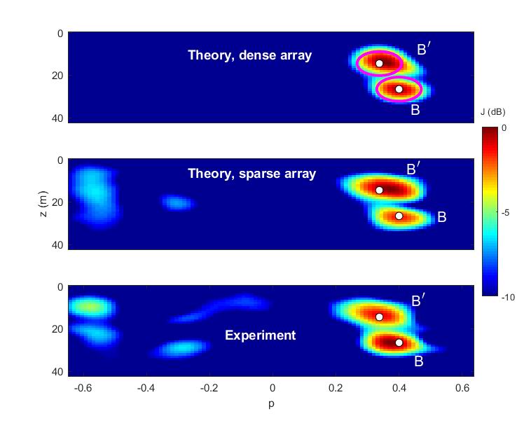
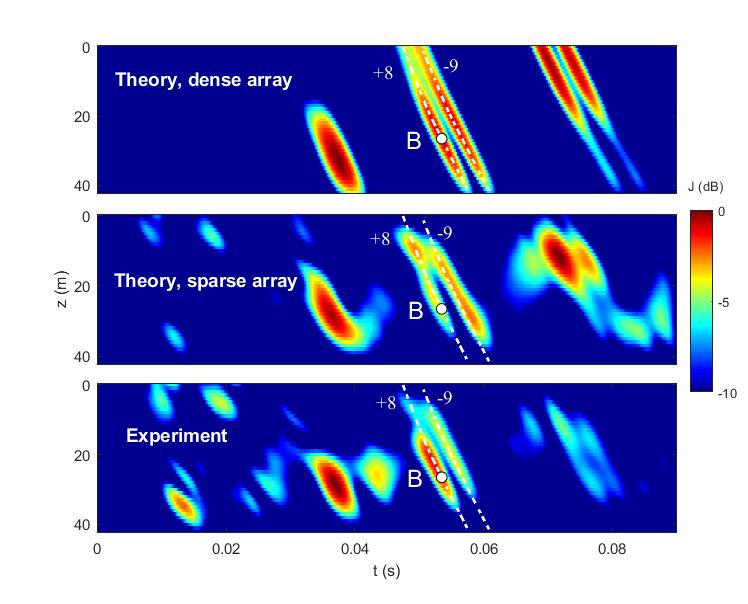
Similar results for a distance of 905 m are shown in Figs. 12-14. In these figures we see the sections of the distribution $J\left(z,p,t\right)$ by planes passing through the point $\left(z_{B},p_{B},t_{B}\right)$ representing the arrival of ray $B$, where $z_{B}$ = 27.3 m, $p_{B}$ = 0.4, $t_{B}=$ 0.05 s. Figures 12, 13, and 14 present the sections by the planes $t=t_{B}$, $z=z_{B}$, and $p=p_{B}$, respectively. The white circles show the arrivals of rays $B$ and $B^{\prime}$. Points B and B’ belong to segments +8 and -9, respectively. Therefore, the magenta ellipses in Fig. 12 and white dotted lines in Fig. 14 are built for these segments. In the top panel of Fig. 13 we see that, unlike the results obtained for the distance of 380 m (Fig. 10), even when using a dense array covering the entire vertical section, the contributions of not all beams are resolved in the $z=z_{B}$ plane.

The results presented in Figs. 9-14, as well as similar results obtained for other three distances, show that the intensity distribution $J(z,p,t)$, even in the absence of complete information about the bottom parameters, can be satisfactory predicted using the simplest range-independent environmental models.

Figure 12: Cross section of the intensity distribution $J\left(z,p,t\right)$ at a distance of 905 m by the plane $t=t_{B}$. Top and middle panels: numerical simulations. Bottom panel: experiment. The white circles indicate the arrivals of rays B and B’ in the phase plane. Magenta ellipses in the upper panel show the boundaries of fuzzy segments +8 (around point B) and -9 (around point B’) in the plane $t=t_{B}$.

Figure 13: Cross section of the intensity distribution $J\left(z,p,t\right)$ at a distance of 905 m by the plane $z=z_{B}$. Top and middle panels: numerical simulations. Bottom panel: experiment. The white circles indicate the arrival of ray $B$. In the upper panel, next to each local maximum, the identifier of the corresponding segment is indicated.

Figure 14: Cross section of the intensity distribution $J\left(z,p,t\right)$ at a distance of 905 m by the plane $p=p_{B}$. Top and middle panels: numerical simulations. Bottom panel: experiment. The white circle shows the arrival of ray $B$. The white dotted lines show the projections of segments +8 and -9.

4.2 Source localization

Comparison of theory and experiment confirms our assumption that the intensity distribution in the phase space is localized mainly inside the fuzzy ray line introduced in Sec. 3.4. This circumstance can be used to estimate the coordinates of the source, that is, to solve the localization problem.

Our idea is as follows. Consider a set of possible source positions $\mathbf{r}$ forming a search grid. Using the standard ray code, for each position $\mathbf{r}$, we find all the beams of rays escaping this point and hitting the antenna. Based on this calculation, we construct the function $W\left(z,p,t;\mathbf{r}\right)$, which is equal to 1 if the point $(z,p,t)$ is inside the fuzzy ray line, and 0 otherwise. Introduce the uncertainty function

$$K\left(\mathbf{r}\right)=\max_{\tau}\int dpdzdt~{}J\left(z,p,t\right)W\left(z,p,t+\tau;\mathbf{r}\right),$$ (14)

where $J\left(z,p,t\right)$ is the intensity distribution of the registered field. It is natural to expect that the function $K\left(\mathbf{r}\right)$ will take its maximum value at the point $\mathbf{r}$, which coincides with the actual source position $\mathbf{r}_{s}$. In this case, the weight function $W\left(z,p,t+\tau;\mathbf{r}\right)$ provides integration over those areas of the phase space where $J$ takes the largest values. A search by $\tau$ is necessary, since it is assumed that we do not know the exact time of signal emission. The desired estimate of the source position has the form

$$\mathbf{\hat{r}}_{s}=\arg\max_{\mathbf{r}}K\left(\mathbf{r}\right).$$

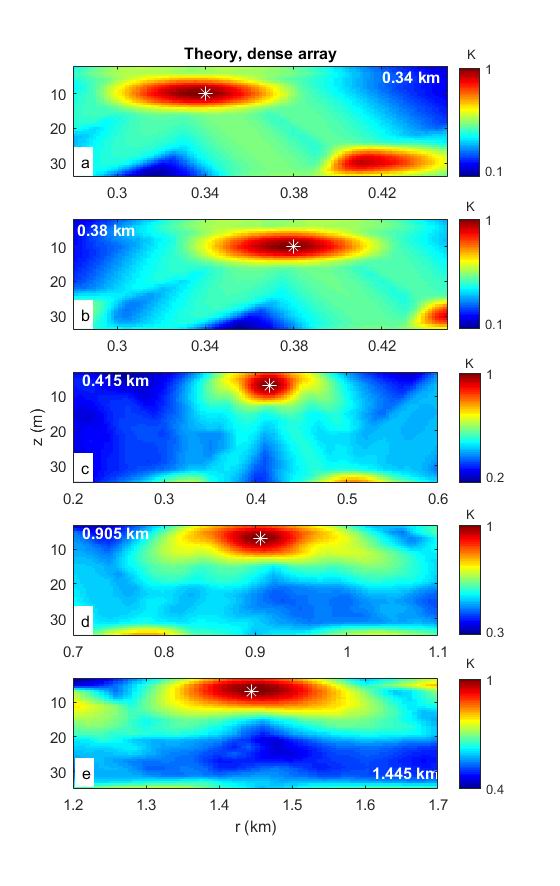
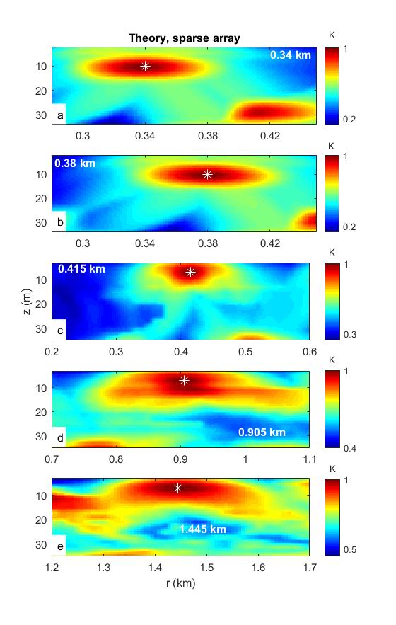
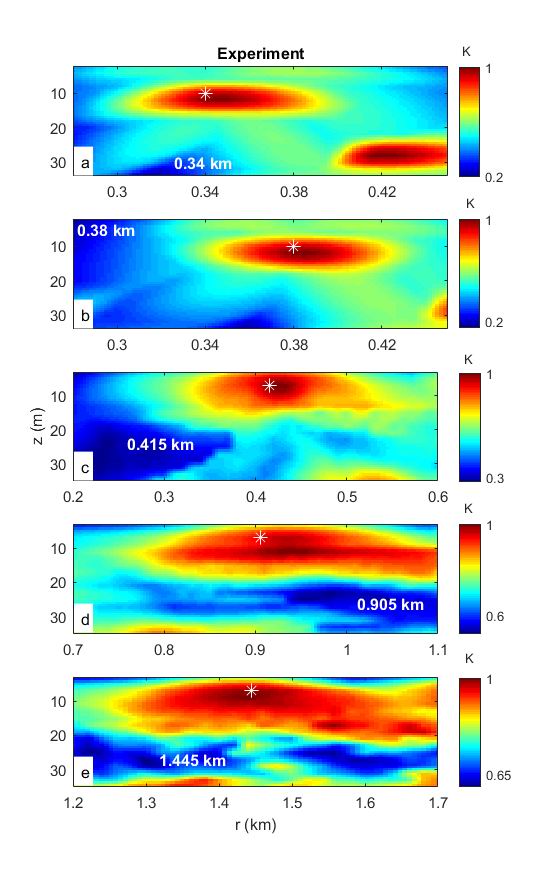
Let us apply this approach to estimate the source coordinates from the data of acoustic measurements. In our range-independent waveguide model, the uncertainty function (14) has two arguments $r$ and $z$. Function $J\left(z,p,t\right)$ in the integrand in (14) is calculated by the coherent state expansion of field $u(z,t)$ in the vertical section of the waveguide at the location of the receiving array. Figure 15 shows the uncertainty functions $K\left(r,z\right)$, obtained using the fields $u(z,t)$ calculated theoretically on a dense vertical array covering the entire vertical section of the waveguide at 340 m (a), 380 m (b), 415 m (c), 905 m (d), and 1440 m (e). Similar calculations of the uncertainty functions were carried out using the fields $u(z,t)$ reconstructed from the signals recorded by 10 hydrophones. Figures 16 and 17 show the results obtained for hydrophone signals calculated theoretically and measured in experiments, respectively. It is seen that in all cases the white asterisk, indicating the point of the actual source position, is located inside the main peak of the uncertainty function $K\left(r,z\right)$.

Figure 15: Uncertainty functions $K\left(r,z\right)$ for the observation distances of 340 m (a), 380 m (b), 415 m (c), 905 m (d) and 1440 m (e). The functions are obtained using the theoretical calculation of the field on a dense receiving array covering the entire vertical section of the waveguide. The white asterisk indicates the actual source position.

Figure 16: The same as in Fig. 15, but for a receiving array of 10 elements.

Figure 17: The same as in Fig. 15, but with the uncertainty functions computed using the experimental data.

5 Conclusion

This work continues the analysis of the phase space representation of the sound field in an underwater waveguide started in Refs. [5, 6]. Such a description of the wave field is unconventional for underwater acoustics. Our interest in this representation is due to the fact that the field distribution in the 3D phase space ’depth - angle - time’ is more regular and predictable than in the 2D space ’depth - time’. The point is that there are no multipaths and no problems with caustics in the phase space [11]. Refs. [5, 6] argue that when solving inverse problems, the transition from the configuration space to the phase space makes it possible to relax the requirements for the accuracy of the environmental model.

The phase space representation of the sound field in the vertical section of the waveguide is introduced using the coherent state expansion. This allows one to resolve the contributions of waves simultaneously in terms of depth and arrival angle, that is, to isolate signals arriving in a relatively small depth interval at grazing angles from a relatively small angular interval. The considered approach makes it possible to find the distributions of the field amplitude and intensity in the phase space. Explicit expressions for calculating these distributions are given by (5) and (11).

Our attention was mainly focused on the analysis of the intensity distribution in the phase space $J\left(z,p,t\right)$. Since the sound field was recorded using the array of only ten sparsely spaced elements, in the processing we analyzed only the field components at frequencies in the lower part of the emitted signal band. Comparison of the results presented in the upper and middle panels of Figs. 9-14 shows that the undersampling, even at low frequencies, causes some errors in the intensity calculation. However, there is good agreement between theory and experiment. Since the theoretical description is based on a highly idealized environmental model, this fact confirms our assumption that the field intensity distribution in the phase space is weakly sensitive to variations in the waveguide parameters.

An important implication of the theory is that the intensity distribution is localized in the area of the phase space, which we call the fuzzy ray line. Figure 8 show that these area occupy a relatively small part of the phase space available for rays in our waveguide model. In Sec. 4.2 it is shown that this circumstance can be used to solve the problem of source localization in a waveguide.

Finally, we note one more important application of the coherent state expansion. Section 3.3 shows that it can be used to isolate a component of the total field formed by a given beam of rays. In the present paper there is no separate section describing the application of this procedure, generalizing the standard procedure for forming a lobe of directivity pattern in free space. The point is that in our example, isolating the contribution from the ray beam is actually equivalent to calculating the cross section of the intensity distribution $J\left(z,p,t\right)$ by the plane $p=$ const. In the cross sections presented in Figs. 11 and 14 we clearly see the isolated contributions of beams of rays with identifiers +5 and -6 at a distance of 380 m and with identifiers +8 and -9 at a distance of 905 m, respectively.

References

- [1] F.B. Jensen, W.A. Kuperman, M.B. Porter, and H. Schmidt, Computational Ocean Acoustics. New York, NY, USA: Springer, 2011.
- [2] P.C. Etter, Underwater acoustic modeling and simulation. Boca Raton, USA: CRC Press, 2018.
- [3] E.S. Livingston, J.A. Goff, S. Finette, P. Abbot, J.F. Lynch, and W.S. Hodgkiss, "Guest editorial capturing uncertainty in the tactical ocean environment," J. Ocean Eng., vol. 31, no. 2, pp. 245–248, 2006.
- [4] Y. Le Gall, S.E. Dosso, F-X. Socheleau, and J. Bonnel, "Bayesian source localization with uncertain Green’s function in an uncertain shallow water ocean," J. Acoust. Soc. Am., vol. 139, no. 3, pp. 993–1004, 2016.
- [5] A.L. Virovlyansky, "Stable components of sound fields in the ocean," J. Acoust. Soc. Am., vol. 141, no. 2, pp. 1180–1189, 2017.
- [6] A.L. Virovlyansky, A.Yu. Kazarova, and L.Ya. Lyubavin, "Matched field processing in phase space," J. Ocean Eng., vol. 45, no. 4, pp. 1583–1593, 2020.
- [7] R.J. Glauber, Quantum Theory of Optical Coherence. Selected Papers and Lectures. Weinheim, Germany: Wiley-VCH, 2007.
- [8] J.R. Klauder and E.C.G. Sudarshan,Fundamentals of quantum optics. New York, USA: W.A. Benjamin, 1968.
- [9] W.P. Schleich, Quantum Optics in Phase Space. Berlin, Germany: Wiley-VCH, 2001.
- [10] H. Goldstein, C.P. Poole, and J.L. Safko, Classical mechanics. San Francisco, USA: Addison-Wesley, 2000.
- [11] M.A. Alonso, "Rays and waves," Phase-space optics. In M. Testorf, B. Hennely, and J.Ojeda-Castaneda, editors, chapter 8, pp. 237–277, New York, USA: McGraw-Hill, 2010.
- [12] A.L. Virovlyansky, "Beamforming and matched field processing in multipath environments using stable components of wave fields," J. Acoust. Soc. Am., vol. 148, no. 4, pp. 2351–2360, 2020.
- [13] L. Liu, K. Sotiri, Y. Duck et al, "The control of sediment gas accumulation on spacial distribution of ebullition in Lake Kinneret," Geo-Marine Letters, [Online]. Available: https://doi.org/10.1007/s00367-019-00612-z
- [14] J.C. Papp, J.C. Preisig, and A.K. Morozov, "Physically constrained maximum likelihood mode filtering," J. Acoust. Soc. Am., vol. 127, no. 4, pp. 2385-2391, 2010.
- [15] L.M. Brekhovskikh and Yu.P. Lysanov, Fundamentals of Ocean Acoustics. New York, USA: Springer-Verlag, 2003.
- [16] D. Makarov, S. Prants, A. Virovlyansky, and G. Zaslavsky, Ray and wave chaos in ocean acoustics. New Jersey, USA: Word Scientific, 2010.
- [17] L.D. Landau and E.M. Lifshitz, Quantum mechanics. Oxford, England: Pergamon Press, 1977.