Blindly Deconvolving
Super-noisy Blurry Image Sequences

Abstract

Image blur and image noise are imaging artifacts intrinsically arising in image acquisition. In this paper, we consider multi-frame blind deconvolution (MFBD), where image blur is described by the convolution of an unobservable, undeteriorated image and an unknown filter, and the objective is to recover the undeteriorated image from a sequence of its blurry and noisy observations. We present two new methods for MFBD, which, in contrast to previous work, do not require the estimation of the unknown filters.

The first method is based on likelihood maximization and requires careful initialization to cope with the non-convexity of the loss function. The second method circumvents this requirement and exploits that the solution of likelihood maximization emerges as an eigenvector of a specifically constructed matrix, if the signal subspace spanned by the observations has a sufficiently large dimension.

We describe a pre-processing step, which increases the dimension of the signal subspace by artificially generating additional observations. We also propose an extension of the eigenvector method, which copes with insufficient dimensions of the signal subspace by estimating a footprint of the unknown filters (that is a vector of the size of the filters, only one is required for the whole image sequence).

We have applied the eigenvector method to synthetically generated image sequences and performed a quantitative comparison with a previous method, obtaining strongly improved results.

Keywords deconvolution  $\cdot$ image restoration  $\cdot$ inverse problems  $\cdot$ maximum likelihood

1 Introduction

Image acquisition is an indispensable step in many technical applications, including digital photography (e.g., [1]), visual inspection of industrial devices and other structures (e.g., [2, 3, 4]), surveillance (e.g., [5, 6, 7]), and biomedical image analysis (e.g, [8, 9, 10]). Despite of a broad range of applications, the acquisition of images is an error-prone task: Challenging imaging conditions like imperfections of the optical systems, camera shake, low-light conditions, or high relative velocities are common causes of imaging artifacts which are perceived as blurriness. In addition, the acquired or observed image data is often deteriorated by image noise (see Figure 1). In some application areas such as digital photography, noise can be suppressed by longer exposures, which, however, comes at the cost of increased blurriness. On the opposite, shorter exposures tend to yield observations which are less blurry, but noisier. So, at the end of the day, image restoration techniques are required.

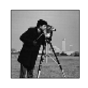
(a) Undeteriorated observation

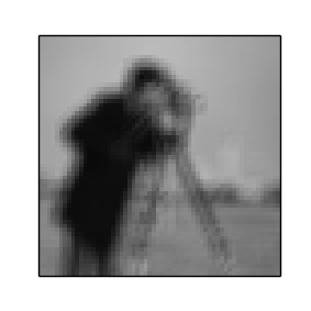
(b) Blurry observation

(c) Blurry and noisy observation

Figure 1: Common imaging artifacts (synthetically generated).

This paper is widely based on the unpublished master’s project of Kostrykin [11]. Throughout the paper, we assume that the image blur is invariant w.r.t. the location within an image. Using this assumption, it is convenient to describe the blur of an observed image by the convolution $x\ast a$ of an unobservable and undeteriorated ground truth $x$ and some filter $a$, where the latter characterizes the blur. Our work can be extended to tackle spatially variant blur using [12].

The recovery of the undeteriorated image $x$ from its blurry observation $y$ is called deconvolution, where it is $y=x\ast a$, in the noise-free case. In practical applications, not only $x$, but also the filter $a$ is unknown, which is referred to as blind deconvolution. The blind deconvolution problem is ill-posed: For instance, $y=x$ with $a$ being the identity element of convolution solves the linear system $y=a\ast x$ for any observation $y$ (but this is not a meaningful solution).

The blind deconvolution problem becomes tractable, either by making prior assumptions regarding $a$ and $x$, or by taking more than just one observation of the same $x$ into account. The recovery of $x$ from a sequence of $n$ observations $y_{1},\dots,y_{n}$ is called multi-frame blind deconvolution (MFBD). We will write $a_{i}$ to denote the filter, which characterizes the $i$-th observation $y_{i}$ of $x$. Note that displacements of the observed object w.r.t. the imaging system within the image sequence are tolerable since translations can be expressed by convolution. In this paper, we consider the case that the observations are very noisy, but also $n$ is very large. Such a setting is common in, for example, astronomical imaging.

1.1 Notational conventions

We use the following notation throughout this paper.

Functions. For notation of function values, we write square brackets to indicate that the domain of a function is discrete, and round brackets to indicate that it is continuous. We also implicitly consider functions with discrete domain and finite support as column vectors (tuples). Consequently, we also use square brackets to represent components of vectors.

Matrices and vectors. For explicit notation of vectors and matrices, we use square brackets like $\left[y_{1}\,\dots\,y_{n}\right]$ to write a matrix consisting of the columns $y_{1},\dots,y_{n}$, and we use round brackets like $\left(\alpha_{1},\dots,\alpha_{n}\right)$ to write a tuple consisting of the components $\alpha_{1},\dots,\alpha_{n}$ (i.e. a column vector). Superscript $\mathsf{T}$ stands for transposition and $\left\|\cdot\right\|$ implies the $\ell_{2}$ norm.

Probabilities. We write $p\left(y\middle|x,a\right)$ to denote the conditional probability of $y$, given $x$ and $a$.

1.2 Blur through discrete convolution

Although the blurring in image acquisition takes place before the continuous image signal is discretized by the digital image sensor, and is thus subject to continuous mechanics, it nevertheless can be modeled through discrete convolution (for justification, see Section B3.2 in [13]). Discrete convolution is a commutative operation, that takes two images represented by functions $g,h$ and yields a new one. One of the two input images is called the filter. However, due the commutativity, the naming is context-dependent. Formally, we rely on the definition from [14] for discrete convolution,

$$\left(g\ast h\right)\left[t\right]=\sum_{k=-\infty}^{\infty}g\left[t-k\right]\cdot h\left[k\right]\text{,}$$ (1.1)

with two functions $g,h\colon\mathbb{Z}\to\mathbb{R}$. To simplify notation, we will only describe the one-dimensional case, whenever the two-dimensional case behaves analogously. Otherwise, the differences will be pointed out.

Given that the functions $g,h$ represent digital images, it is plausible to assume that they have finite support. This motivates considering $g$ and $h$ as vectors of dimensions $N_{g}$ and $N_{h}$, respectively. For algebraic considerations, we will implicitly consider $g,h$ as vectors, obtained by column-wise concatenation of the two-dimensional images which they represent. For an undeteriorated image $x$ and a filter $a$, we see from Eq. (1.1) that the convolution $x\ast a$ is linear in both, $x$ and $a$. Thus, convolution can be written as the matrix-vector-product $a\ast x=Ax$, but also $a\ast x=Xa$, where the matrices $A$ and $X$ are induced by the vectors $a$ and $x$, respectively (this is described in Section 2).

Throughout this paper, we assume that all filters $a_{i}\in\mathbb{R}^{N_{a}}$ are of equal size $N_{a}$, and particularly smaller than the image $x\in\mathbb{R}^{N_{x}}$ in every dimension, which we write as $N_{a}<N_{x}$. We say, that the filter $a$ is a point spread function (PSF), if it neither has negative elements, nor its application to an image changes the image’s brightness, i.e. $\sum_{k}a\left[k\right]=1$.

1.3 Previous approaches

Early work on deconvolution of noisy images included [15, 16]. Richardson [15] derived multiplicative updates for the case of non-blind deconvolution. It was assumed that the object and the image are probability distributions on the pixels. Bayes’ formula together with the definition of conditional probability leads to the update formula. Curiously, the conditional probability of an image pixel given an object pixel is the PSF. A similar derivation was performed by Lucy [16], who also showed how this can be seen as an approximation of likelihood maximization. We refer the reader to [17] for a comprehensive overview of the early work.

A prominent approach specifically for multi-frame blind deconvolution (MFBD) was proposed by Harikumar and Bresler [18]. The authors used the likelihood maximization approach $\hat{a}=\arg\max_{a}\max_{x}p\left(y\middle|x,a\right)$, where $y=\left[y_{1}\,\dots\,y_{n}\right]$ and $a=\left[a_{1}\,\dots\,a_{n}\right]$, and derived the estimate $\hat{a}=\beta\cdot\arg\min_{a}a^{\mathsf{T}}R\,a$ of the filters, where $\beta=\left\|\hat{a}\right\|$ is a positive factor and the matrix $R$ can be constructed from the true and unknown filters $a$. They constrained that the norm of $\arg\min_{a}a^{\mathsf{T}}R\,a$ should be $1$ to avoid the trivial solution $\hat{a}=0$ and showed that $\pm\hat{a}/\beta$ are the eigenvectors of $R$, which correspond to its smallest eigenvalue. To determine these eigenvectors, the authors used an approximation of the matrix $R$ which was refined iteratively. It is easy to recover the norm of each filter $\hat{a}_{i}$ using the assumption that it is a PSF. However, each iteration for the refinement of the estimated matrix $R$ requires solving a least squares problem that involves the whole sequence of observations, rendering the method infeasible for large $n$.

Šroubek and Milanfar [19] observed that the method of Harikumar and Bresler [18] fails in the presence of noise and addressed this issue via regularization. They employed a prior for $x$ which favors a sparse gradient. For the regularization of the filters $a$, they derived another matrix $R_{\Delta}$ so that $\hat{a}\approx\arg\min_{a}a^{\mathsf{T}}R_{\Delta}a$; but in contrast to the work of [18], their $R_{\Delta}$ does not depend on the unknown filters $a$ and is robust to noise. They minimized the resulting objective function w.r.t. $x$ and $a$ alternatingly. However, the $n\,N_{a}\times n\,N_{a}$ matrix $R_{\Delta}$ is dense, which makes the method impractical for large $n$.

To cope with large image sequences, Harmeling et al. [20] proposed an online algorithm for MFBD, which considers only a single observation per iteration. The authors used the loss function $\sum_{i}^{n}\left\|y-x\ast a_{i}\right\|^{2}$, whose minimization is equivalent to the maximization of the likelihood $p\left(y\middle|x,a\right)$ under mild conditions, and derived multiplicative updates for $x$ and $a$.

The abovementioned methods have in common that the filters $a$ are determined alongside, although only the undeteriorated image $x$ is of interest. This means that the parameter space is larger than required (a filter needs to be estimated for each image of the sequence, which is a potentially very large number), causing additional computational cost. To the best of our knowledge, this concerns all previously developed methods for MFBD.

1.4 Contributions

In this paper, we propose two methods which eliminate the need for estimating the filters $a$ in order to determine the undeteriorated image $x$. This not only has the advantage that fewer variables must be computed, but also that, in the special cases described below, the undeteriorated image $x$ can be determined without alternating optimization schemes.

In our work, the estimate $\hat{x}_{\ast}$ of the undeteriorated image $x$ appears as an eigenvector of a specific matrix. We show, that this matrix is fully determined solely by the observations, and its eigenvector $\hat{x}_{\ast}$ maximizes the likelihood of the observations, when two specific conditions are met:

1. The first condition is that the observations are noise-free – however, we argue that this condition is also attained asymptotically in the presence of noise, if a sufficiently large number $n$ of observations is taken into account. This is achieved by a subspace technique [21], that makes the proposed methods cope with any noise level as long as $n$ is sufficiently large.

2. The second condition concerns the filters which characterize the blur of the observed images and requires that they span a space of a sufficiently large dimension. We describe a pre-processing step which artificially generates additional observations, making this condition more likely to be fulfilled. Still, this is insufficient in specific cases, and the proposed method falls back to an alternating optimization scheme then.

In Section 2, we briefly describe the theoretical foundations of our work. In Section 3, we derive a method based on likelihood maximization which directly determines the undeteriorated image $x$ without estimating the filters $a$. The loss function of this method is non-convex and direct minimization requires reliable initialization. In Section 4, we describe the second method, which exploits that the same solution emerges as an eigenvector of a specific matrix. The method is applied to synthetically generated image sequences, and the obtained results are compared to those achieved using a previous method [20]. Finally, we discuss its advantages and limitations in Section 5.

2 Foundations

2.1 Valid convolution and associativity

The computation of $x\ast a$ can be done efficiently using the discrete Fourier transform (DFT) of $x$ and $a$. Since the computation of the DFT of $x$ (or $a$) is a linear operation, we can write it as the matrix-vector-product $Fx$, where $F$ is the DFT matrix (see, e.g., [22]). We denote the Hermitian conjugate of $F$ as $F^{\mathsf{H}}=\overline{F}{\,}^{\mathsf{T}}$, where $\overline{F}$ for is the complex conjugate of $F$. The matrix $F$ is unitary, i.e. $F^{\mathsf{H}}=F^{-1}$, thus $F^{\mathsf{H}}$ expresses the inverse DFT of the vector to its right.

If $x$ represents an image section from a larger, $N_{x}$-periodical image, then the discrete version of the widely known convolution theorem (see, e.g., Theorem B3.2 in [13]) states that, the expression

$$a\ast x=F^{\mathsf{H}}\left(Fx\odot FI_{a}a\right)$$ (2.1)

is a period of the periodical, convolved image. The matrix $I_{a}$ pads the vector to its right with zeros and $\odot$ stands for element-wise multiplication. The computation of $a\ast x$ through Eq. (2.1), which is called circular convolution, causes artifacts at the boundaries when used for non-periodic signals.

To cope with that, we only keep the valid section of $a\ast x$ computed by Eq. (2.1), which is the section where the periodicity artifacts do not occur. This is referred to as valid convolution and we write

$$a\ast_{\text{valid}}x=I_{y}^{\mathsf{T}}\left(a\ast x\right)\stackrel{{\scriptstyle\hbox to0.0pt{\eqref{eq:convolution:circ}\hss}}}{{=}}I_{y}^{\mathsf{T}}F^{\mathsf{H}}\left(Fx\odot FI_{a}a\right)\text{,}$$ (2.2)

where the matrix $I_{y}^{\mathsf{T}}$ crops $a\ast x$ so that its size equals $N_{y}=N_{x}-N_{a}+1$. Using Eq. (2.2), we can write the matrix-vector-products $Ax$ and $Xa$ using the matrices $A$ and $X$ defined as functions of $a$ and $x$,

$$A\!\left(a\right) =I_{y}^{\mathsf{T}}F^{\mathsf{H}}\operatorname{Diag}\left(FI_{a}a\right)F,$$ (2.3)

$$X\!\left(x\right) =I_{y}^{\mathsf{T}}F^{\mathsf{H}}\operatorname{Diag}\left(Fx\right)FI_{a},$$ (2.4)

respectively. This directly leads to the curious rule of associativity

$$b\ast_{\text{valid}}\left(a\ast_{\text{valid}}x\right)=\left(b\ast_{\text{full}}a\right)\ast_{\text{valid}}x\text{,}$$ (2.5)

where $b\in\mathbb{R}^{N_{b}}$ is another filter and

$$b\ast_{\text{full}}a=F^{\mathsf{H}}\left(FI_{b}b\odot FI_{a}a\right)$$ (2.6)

denotes full convolution, a different way of avoiding periodicity artifacts. The matrices $I_{b}$ and $I_{a}$ zero-pad $b$ and $a$ to the size of the result, that is $N_{b}+N_{a}-1$. Note that valid convolution yields an image smaller than $x$, whereas full convolution yields an image larger than $x$.

2.2 Multi-frame forward model

Below, we write $x_{\text{true}}$ to explicitly denote the unknown and undeteriorated ground truth image (for simplicity, this was denoted by a simple $x$ in Section 1). Following [18], we assume that an observation $y_{i}$ of $x_{\text{true}}$ is the additive superposition of two unobservable quantities. These are the noise-free, blurry image $\tilde{y}_{i}=a_{i}\ast_{\text{valid}}x_{\text{true}}$ and the noise $\varepsilon_{i}$:

$$y_{i}=a_{i}\ast_{\text{valid}}x_{\text{true}}+\varepsilon_{i}=X\!\left(x_{\text{true}}\right)a_{i}+\varepsilon_{i}$$ (2.7)

Figure 2 illustrates this modeling. We further assume that $\varepsilon_{i}$ is additive white Gaussian noise (AWGN).

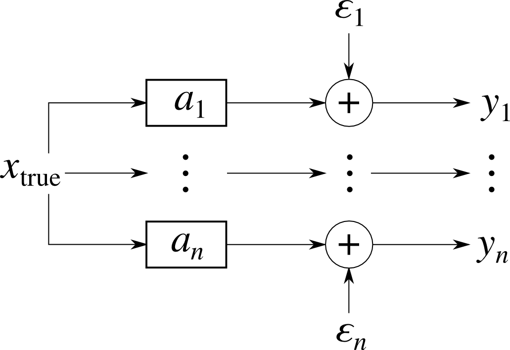
Figure 2: The multi-frame forward model by Harikumar and Bresler [18].

The $N_{y}\times N_{a}$ matrix $X\!\left(x\right)$ in Eq. (2.7) is structured like

$$X\!\left(x\right)=\left[\begin{array}[]{cccc}x_{N_{a}}&x_{N_{a}-1}&\cdots&x_{1}\\ \vdots&\vdots&&\vdots\\ x_{N_{x}}&x_{N_{x}-1}&\cdots&x_{N_{x}-N_{a}+1}\end{array}\right]\text{,}$$ (2.11)

that is, the range (column space) of $X$ is spanned by all $N_{y}$-sized sections of $x$, which are $N_{a}$ in count. This establishes the following intuitive view of Eq. (2.7): Any noise-free observation of $x$ is a linear combination of all $N_{y}$-sized sections of $x$, and $a_{i}$ corresponds to the weights of the combination (i.e. how much each section contributes to the observation).

The dimension $N_{a}$ of the filters $a_{i}$ is a parameter of the model. It controls the number of adjacent pixels, any filter can put into relation at most. Thus, the bigger we choose $N_{a}$, the higher the more blur the model is capable to explain.

2.3 Identifying the signal subspace

Repetitive observation of $x_{\text{true}}$ yields a sequence of $N_{y}$-dimensional vectors according to Eq. (2.7). In the noise-free case, there are at most $N_{a}$ degrees of freedom. Since $y_{i}$ depends linearly on $a_{i}$, the vectors $\tilde{y}_{1},\dots,\tilde{y}_{n}$ span an $m$-dimensional subspace of $\mathbb{R}^{N_{y}}$, where $m\leq N_{a}$ and $N_{a}$ may be much smaller than $N_{y}$. Moulines et al. [21] called this the signal subspace. There are at least three reasons, why we should expect $m<N_{a}$:

1. The model parameter $N_{a}$ might be overestimated.

2. Natural PSFs aren’t rectangular.

3. Even if variance is encountered in all pixels of the filters, $m<N_{a}$ will still hold for filters which are sampled from a PSF subspace, i.e. a subspace of $\mathbb{R}^{N_{a}}$.

Note that the last reason holds particularly if, but not only if, $n<N_{a}$ (i.e. the number of observations is too small).

Note that $m$ cannot be larger than the dimension of the PSF subspace. Moreover, as we see from

$$\operatorname{rk}\left[\tilde{y}_{1}\,\dots\,\tilde{y}_{n}\right]\;\stackrel{{\scriptstyle\hbox to0.0pt{\eqref{eq:model}\hss}}}{{=}}\;\operatorname{rk}\left[Xa_{1}\,\dots\,Xa_{n}\right]\text{,}$$ (2.12)

the dimensions of the signal subspace and the PSF subspace are equal if $\operatorname{rk}X=N_{a}$. This property means that none of the $N_{y}$-sized sections of $x_{\text{true}}$ are linearly dependent. Harikumar and Bresler [18] called those images, which this property holds for, persistently exciting. We assume that $x_{\text{true}}$ is persistently exciting for the rest of this paper.

2.3.1 Noise-free case

Moulines et al. [21] proposed identification of the signal subspace by a process similar to performing PCA (see, e.g., [23]) without mean subtraction on the noise-free observations $\tilde{Y}=\left[\tilde{y}_{1}\,\dots\,\tilde{y}_{n}\right]$. The eigenvalue decomposition (EVD)

$$\frac{1}{n}\tilde{Y}\tilde{Y}^{\mathsf{T}}=U\Lambda U^{\mathsf{T}}$$ (2.13)

of the empirical covariance matrix $\frac{1}{n}\tilde{Y}\tilde{Y}^{\mathsf{T}}$ of the noise-free observations $\tilde{Y}$ with non-negative eigenvalues $\Lambda=\operatorname{Diag}\lambda$ induces the matrix $U$. If we put the eigenvalues into descending order $\lambda_{i}\geq\lambda_{i+1}$, then the first columns of $U$ correspond to the directions with the greatest variance. The signal subspace is then spanned by the $m$ first columns of $U$, and $m$ equals the number of non-zero eigenvalues.

2.3.2 Noisy case

If the number $n$ of observations is sufficiently large, then the signal subspace is also identifiable in the presence of noise. To understand this, we will look at how the additive noise vectors $E=\left[\varepsilon_{1}\,\dots\,\varepsilon_{n}\right]$ influence the covariance matrix of the noisy observations. Writing $Y=\left[y_{1}\,\dots\,y_{n}\right]$, the covariance matrix resolves to

$$\frac{1}{n}YY^{\mathsf{T}}=\frac{1}{n}\tilde{Y}\tilde{Y}^{\mathsf{T}}+\frac{1}{n}\tilde{Y}E^{\mathsf{T}}+\frac{1}{n}E\tilde{Y}^{\mathsf{T}}+\frac{1}{n}EE^{\mathsf{T}}\text{.}$$ (2.14)

For $n\to\infty$, the terms $\frac{1}{n}\tilde{Y}E^{\mathsf{T}}$ and $\frac{1}{n}E\tilde{Y}^{\mathsf{T}}$ both tend to $0$, because $\tilde{Y}$ and $E$ are uncorrelated. Furthermore, since we know that the noise $E\sim\mathcal{N}\left(0;I\sigma^{2}\right)$ is white by assumption in Section 2.2, we conclude that $\frac{1}{n}EE^{\mathsf{T}}\xrightarrow{n\to\infty}I\sigma^{2}$. Then, plugging the decomposition from Eq. (2.13) into Eq. (2.14) yields

$$\lim_{n\to\infty}\frac{1}{n}YY^{\mathsf{T}}=U\left(\Lambda+\sigma^{2}I\right)U^{\mathsf{T}}\text{.}$$ (2.15)

The matrix $\Lambda+\sigma^{2}I$ is diagonal. Thus, Eq. (2.15) equals the EVD of the covariance matrix of the noisy observations for $n\to\infty$. Notably, the eigenvectors of the EVD are the same as in the noise-free case: This means that for a sufficiently large number of observations, the $m$ first eigenvectors of the covariance matrix $\frac{1}{n}YY^{\mathsf{T}}$ span the same subspace, as the unobservable noise-free observations $\tilde{y}_{1},\dots,\tilde{y}_{n}$.

In practice, we have to rely on a finite number of observations. For any fixed $n$, the matrix $\frac{1}{n}EE^{\mathsf{T}}$ deviates the more from diagonal shape, the higher the noise level is. As a consequence, the EVD of $\frac{1}{n}YY^{\mathsf{T}}$ also deviates from Eq. (2.15), and we say that the obtained eigenvectors are misaligned (w.r.t. the ideal eigenvectors of the noise-free observations).

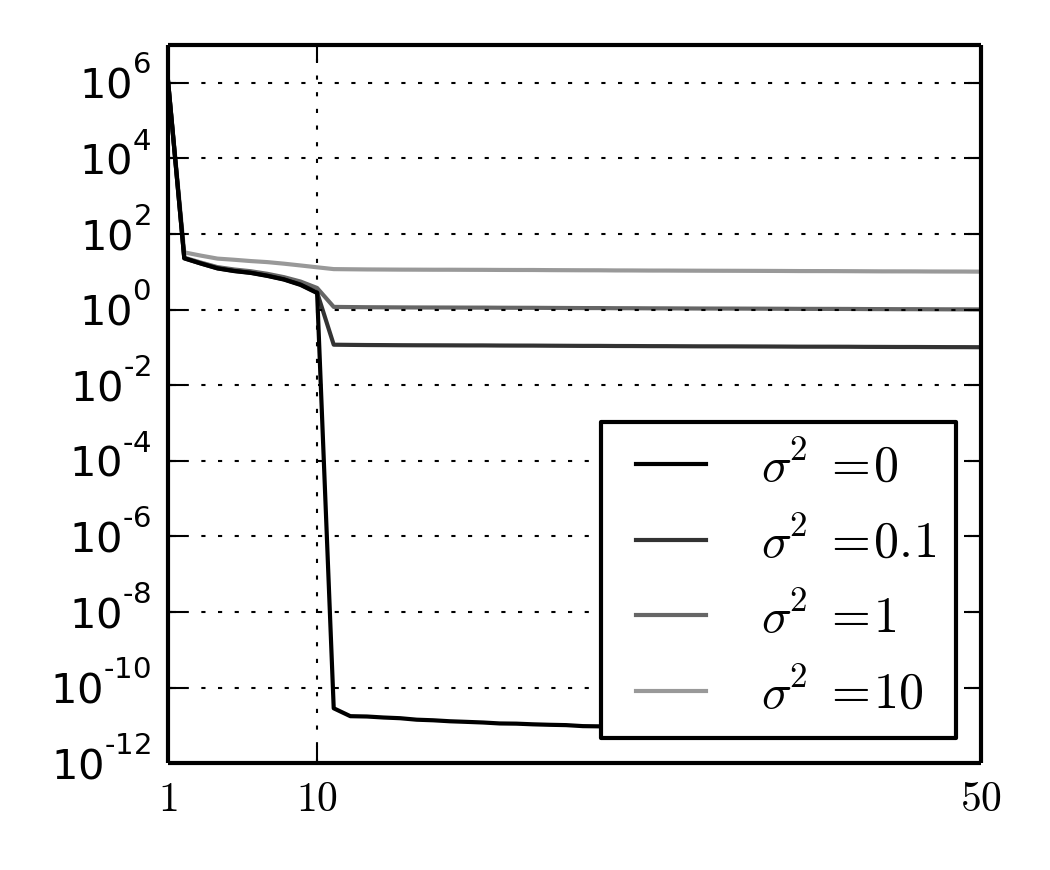
(a) Eigenvalues by noise level

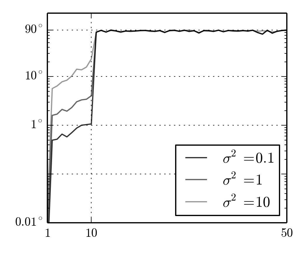
(b) Misalignment of the eigenvectors (in degrees)

Figure 3: The impact of noise on the EVD of the covariance matrix $\frac{1}{n}YY^{\mathsf{T}}$ using $m=10$.

Figure 3 visualizes this for $n=10{,}000$ artificial observations, randomly generated accordingly to Eq. (2.7) using $m=10$, $N_{a}=70$, $N_{y}=1000$, and a ground truth vector $x_{\text{true}}$ with values distributed uniformly between $0$ and $255$. In Figure 3a, the eigenvalues $\lambda_{i}\geq\lambda_{i+1}$ of the covariance matrix $\frac{1}{n}YY^{\mathsf{T}}$ are plotted for different noise levels. The kink at the $10$-th eigenvalue marks the signal subspace dimension $m$. It can be seen that the kink is less clear for higher noise levels. The large drop-off after the first eigenvalue in all four curves in Figure 3a occurs because the vectors $y_{i}$ are not zero-mean. The eigenvector, which corresponds to the first eigenvalue, points roughly towards the mean of the observations. Since all other eigenvectors must be orthogonal, the corresponding eigenvalues must be of lower magnitude. Figure 3b shows that the misalignments of the eigenvectors is larger for higher noise levels. It can also be seen that eigenvectors, which correspond to greater eigenvalues, tend to be more reliable (i.e. less affected by noise).

2.3.3 Application to image data

Figure 4c illustrates the characteristics of the signal subspace described above for synthetic image data comprising $n=2500$ noisy observations. The observations $y_{1},\dots,y_{n}$ were created from the ground truth image in Figure 1a, sampled down to $N_{x}=64\times 64$, and using randomly generated PSFs with $m=25$. An exemplary observation is shown in Figure 4a. The eigenvector $u_{1}$ in Figure 4b, which corresponds to the greatest eigenvalue, is very blurry and noise-free like the mean of all observations. Figure 4e confirms that the eigenvectors from $u_{m+1=26}$ on do not contain much information regarding the signal subspace but mostly noise.

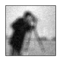
(a) $y_{1}$

(b) $u_{1}$

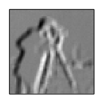
(c) $u_{2}$

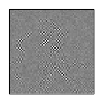
(d) $u_{25}$

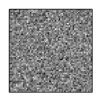
(e) $u_{26}$

Figure 4: An exemplary observation and the corresponding eigenvectors $u_{1},\dots,u_{26}$ of the covariance matrix $\frac{1}{n}YY^{\mathsf{T}}$, where the observations $y_{1},\dots y_{2500}$ were generated according to Eq. (2.7) using random $5\times 5$ PSFs with $m=25$. The pixels in the panels 4a and 4b are non-negative. In the panels 4c–4e, $0$-valued pixels are colored grey, black corresponds to negative values, white to positive.

 …

3 Likelihood maximization approach

In this section, we describe our direct approach for MFBD using a non-convex loss function and without estimating the filters. We first describe the estimate $\hat{x}_{\mathsf{n}}$ of the ground truth $x_{\text{true}}$, which explains the observations $Y=\left[y_{1}\,\dots\,y_{n}\right]$ best in terms of likelihood maximization. The subscript $\mathsf{n}$ indicates, that $\hat{x}_{\mathsf{n}}$ aims to explain the original, noisy input data. Afterwards, we will use the results from Section 2.3.2–2.3.3 to derive the estimate $\hat{x}$ for the noise-free observations using the noisy image data.

Consider the probability $p\left(Y\middle|x,a_{1},\dots,a_{n}\right)$ of the observations, given an undeteriorated image $x$ and the filters $a_{1},\dots,a_{n}$. We confine ourselves to those parameters, for which the condition $p\left(Y\middle|x,a_{1},\dots,a_{n}\right)\neq 0$ holds. Using the monotonicity of the logarithm, we then define

$$\hat{x}_{\mathsf{n}}=\arg\min_{x}\min_{a_{1},\dots,a_{n}}-\ln p\left(Y\middle|x,a_{1},\dots,a_{n}\right)\text{.}$$ (3.1)

Strictly speaking, the minimizer of Eq. (3.1) is not necessarily unique (cf. Section 3.4), so $\hat{x}_{\mathsf{n}}$ is simply defined as an arbitrary minimizer. Assuming that the observations $y_{1},\dots,y_{n}$ are statistically independent, they factorize like $p\left(Y\middle|x,a_{1},\dots,a_{n}\right)=\prod_{i=1}^{n}p\left(y_{i}\middle|x,a_{1},\dots,a_{n}\right)$, and hence

$$\hat{x}_{\mathsf{n}}=\arg\min_{x}\min_{a_{1},\dots,a_{n}}-\sum_{i=1}^{n}\ln p\left(y_{i}\middle|x,a_{1},\dots,a_{n}\right)\text{.}$$ (3.2)

is obtained. In Section 2.2, we assumed that $\varepsilon_{i}$ is AWGN, so Eq. (2.7) takes the form $y_{i}\sim\mathcal{N}\left(a_{i}\ast x;I\sigma^{2}\right)$. Plugging this into Eq. (3.2) in place of $p\left(y_{i}\middle|x,a_{1},\dots,a_{n}\right)$ and dropping those terms from the objective function, which are constant w.r.t. $x$ and $a_{i}$, the likelihood maximization approach for $\hat{x}_{\mathsf{n}}$ boils down to the least-squares problem

$$\hat{x}_{\mathsf{n}}=\arg\min_{x}\min_{a_{1},\dots,a_{n}}\sum_{i=1}^{n}\left\|y_{i}-a_{i}\ast x\right\|^{2}\text{.}$$ (3.3)

So far, the approach is canonical and similar to the work from Harikumar and Bresler [18] and Harmeling et al. [20]. Eq. (3.3) requires the joint optimization w.r.t. $a_{1},\dots a_{n}$ and $x$. We will simplify this problem by confining the parameter space to such $a_{1}\dots a_{n}$, which fulfill the necessary condition for the presence of a minimum in $x$, as described below.

3.1 Closed-form constraint for $a_{i}$

We derive the differential $\mathrm{d}\left\|y_{i}-a_{i}\ast x\right\|^{2}=\mathrm{d}(\left(y_{i}-Xa_{i}\right)^{\mathsf{T}}\left(y_{i}-Xa_{i}\right))$ of the summands of the objective function in Eq. (3.3) using [24], that is

$$\mathrm{d}\left\|y_{i}-a_{i}\ast x\right\|^{2}=-2\left(y_{i}-Xa_{i}\right)^{\mathsf{T}}\mathrm{d}a_{i}\text{.}$$ (3.4)

From Eq. (3.4), we can read off the derivative of $\left\|y_{i}-a_{i}\ast x\right\|^{2}$ w.r.t. $a_{i}$ and use it to find the closed-form optimization constraint on $a_{i}$ for the presence of a minimum,

$$\frac{\partial}{\partial a_{i}}\left\|y_{i}-a_{i}\ast x\right\|^{2}=-2\left(y_{i}-Xa_{i}\right)^{\mathsf{T}}=0\text{,}$$ (3.5)

that is $y_{i}=Xa_{i}$. The null space of $X^{\mathsf{T}}$ is orthogonal to the range of $X$. To see this, consider a vector $v$ from the null space of $X^{\mathsf{T}}$, i.e. $X^{\mathsf{T}}v=0$. This means that $v$ is orthogonal to the range of $X$. Thus, and since $y_{i}\in\operatorname{range}X$, prepending $X^{\mathsf{T}}$ to both sides of the equation doesn’t affect its solution for $a_{i}$:

$$\frac{\partial}{\partial a_{i}}\left\|y_{i}-a_{i}\ast x\right\|^{2}=0\enspace\Leftrightarrow\enspace X^{\mathsf{T}}y_{i}=X^{\mathsf{T}}Xa_{i}$$ (3.6)

The assumption $\operatorname{rk}X=N_{a}$ from Section 2.3 implies that $X^{\mathsf{T}}X$ has full rank [25], so $X^{\mathsf{T}}X$ is invertible and its inverse has full rank too. Thus, prepending $\left(X^{\mathsf{T}}X\right)^{-1}$ to both sides yields another equivalent equation:

$$\left(X^{\mathsf{T}}X\right)^{-1}X^{\mathsf{T}}y_{i}=a_{i}$$ (3.7)

Plugging Eq. (3.7) back into the least squares form in Eq. (3.3) yields an expression, which only needs to be minimized w.r.t. $X$. After resolving the squared norm $\left\|\cdot\right\|^{2}$ using the inner vector product and dropping those summands, which are constant w.r.t. $X$, we finally obtain the estimate

$$\hat{x}_{\mathsf{n}}=\arg\max_{x}\sum_{i=1}^{n}y_{i}^{\mathsf{T}}X\left(X^{\mathsf{T}}X\right)^{-1}X^{\mathsf{T}}y_{i}\text{,}$$ (3.8)

where each $X$ depends linearly on $x$, as described in Section 2.1.

3.2 Denoising

The summands $y_{i}^{\mathsf{T}}X\left(X^{\mathsf{T}}X\right)^{-1}X^{\mathsf{T}}y_{i}$ in Eq. (3.8) are scalar-valued. Using the trace operator $\operatorname{tr}$, the estimate $\hat{x}_{\mathsf{n}}$ is stated equivalently as that $x$ which maximizes $\operatorname{tr}\sum_{i=1}^{n}y_{i}y_{i}^{\mathsf{T}}X\left(X^{\mathsf{T}}X\right)\!{}^{-1}X^{\mathsf{T}}$. Using $YY^{\mathsf{T}}=\sum_{i=1}^{n}y_{i}y_{i}^{\mathsf{T}}$ yields

$$\hat{x}_{\mathsf{n}}=\arg\max_{x}\operatorname{tr}YY^{\mathsf{T}}X\left(X^{\mathsf{T}}X\right)^{-1}X^{\mathsf{T}}\text{.}$$ (3.9)

We now replace $YY^{\mathsf{T}}$ by $U\Lambda U^{\mathsf{T}}$, that is its EVD, but truncate the $N_{y}\times N_{y}$ matrix $U$ after its $m$ first columns, and resolve the trace-operator. This yields the estimate

$$\hat{x}=\arg\max_{x}\sum_{i=1}^{m}\lambda_{i}u_{i}^{\mathsf{T}}X\left(X^{\mathsf{T}}X\right)^{-1}X^{\mathsf{T}}u_{i},$$ (3.10)

which, in view of Section 2.3 and for $n\to\infty$, maximizes the likelihood of the noise-free observations. We will hence refer to $\hat{x}$ as the denoised estimate.

3.3 Geometric interpretation

Note that $\mathrm{P}_{X}=X\left(X^{\mathsf{T}}X\right)^{-1}X^{\mathsf{T}}$ is the projector onto the range of $X$, if $\operatorname{rk}X=N_{a}$ (e.g., [25]), which leads us to

$$\hat{x}=\arg\max_{x}\sum_{i=1}^{m}\lambda_{i}u_{i}^{\mathsf{T}}\mathrm{P}_{X}u_{i}\text{.}$$ (3.11)

The matrix $X^{\mathsf{T}}X$ is symmetric. It is easily seen that its inverse, and consequently also $\mathrm{P}_{X}$, are symmetric too. Since $\mathrm{P}_{X}$ is idempotent, i.e. $\mathrm{P}_{X}^{2}=\mathrm{P}_{X}$, we get $\hat{x}=\arg\max_{x}\sum_{i=1}^{m}\lambda_{i}u_{i}^{\mathsf{T}}\mathrm{P}_{X}^{\mathsf{T}}\mathrm{P}_{X}u_{i}$, which we rewrite as

$$\hat{x}=\arg\max_{x}\sum_{i=1}^{m}\lambda_{i}\left\|\mathrm{P}_{X}u_{i}\right\|^{2}\text{.}$$ (3.12)

Eq. (3.12) dictates, that the longer the projections of the eigenvectors $u_{i}$ onto the range of $X\!\left(x\right)$ are, the better $x$ explains the observations. The term $\left\|\mathrm{P}_{X}u_{i}\right\|\!{}^{2}$ indicates how good $x$ explains variance along $u_{i}$, as Figure 5 illustrates for the simplified case $\operatorname{rk}X=1$. In view of Section 2.3, the factors $\lambda_{i}$ induce the following weighting: A good explanation for larger variance outweighs an equally good explanation for smaller variance.

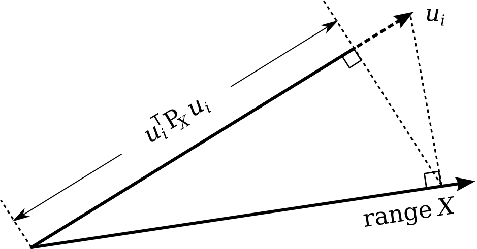
Figure 5: Geometric interpretation of the estimate $\hat{x}$ in Eq. (3.10). The dashed lines indicate projections according to Eq. (3.12) with $\left\|\mathrm{P}_{X}u_{i}\right\|^{2}=u_{i}^{\mathsf{T}}\mathrm{P}_{X}u_{i}$ for the simplified case $\operatorname{rk}X=1$.

3.4 Solution ambiguity

We also see from Eq. (3.12) that, in general, there is an infinite number of solutions $x$: The objective function is invariant w.r.t. the multiplication of $x$ by a scalar $\alpha$ (i.e. the brightness of $\hat{x}$ is ambiguous). This arises from the homogeneity $\left(X\alpha\right)a_{i}=X\left(\alpha a_{i}\right)$ of convolution in the underlying model.

3.5 Gradient ascent

This section demonstrates, that the direct solution of Equation (3.10) is difficult, due to the presence of local extrema in the objective function. To simplify notation, we write $\phi\left(x\right)=\sum_{i=1}^{n}\lambda_{i}\phi_{i}\left(x\right)$ and $\phi_{i}\left(x\right)=u_{i}^{\mathsf{T}}X\left(X^{\mathsf{T}}X\right)\!{}^{-1}X^{\mathsf{T}}u_{i}$ to refer to the objective function in Eq. (3.10) and its summands.

Using [24] and Eq. (2.2) to resolve the matrix $X$, we obtain the differential

$$\mathrm{d}\phi_{i}\left(x\right)=2r_{i}^{\mathsf{T}}I_{y}^{\mathsf{T}}F^{\mathsf{H}}\operatorname{Diag}\left(FI_{a}v_{i}\right)F\mathrm{d}x\text{,}$$ (3.13)

where we abbreviate $v_{i}=\left(X^{\mathsf{T}}X\right)^{-1}X^{\mathsf{T}}u_{i}$ and $r_{i}=u_{i}-Xv_{i}$. Then, we can read off the gradient from Eq. (3.13),

$$\nabla\phi_{i}\left(x\right)=\frac{\partial}{\partial x}\phi_{i}\left(x\right)=2r_{i}^{\mathsf{T}}I_{y}^{\mathsf{T}}F^{\mathsf{H}}\operatorname{Diag}\left(FI_{a}v_{i}\right)F\text{.}$$ (3.14)

To avoid the costly computation of the DFT matrix $F$, we rewrite $\nabla\phi_{i}\left(x\right)$ as $\left(2F^{\mathsf{T}}\operatorname{Diag}\left(FI_{a}v_{i}\right)\overline{F}I_{y}r_{i}\right)^{\mathsf{T}}$. Putting $r_{i}=u_{i}-Xv_{i}$ back in and using that $\phi_{i}=\overline{\phi_{i}}$ since $\phi_{i}$ is real-valued yields

$$\nabla\phi_{i}\left(x\right)=\left(2F^{\mathsf{H}}\operatorname{Diag}\left(\overline{FI_{a}v_{i}}\right)FI_{y}\left(u_{i}-Xv_{i}\right)\right)^{\mathsf{T}}\text{.}$$ (3.15)

The gradient of the objective function $\phi\left(x\right)$ always points into the direction of the steepest ascent. Given an estimate $\hat{x}_{0}$, the gradient ascent iteration $\hat{x}_{t+1}=\hat{x}_{t}+\tau\nabla\phi\left(\hat{x}_{t}\right)$ yields an improved estimate. The parameter $\tau$ controls the step distance per iteration, we used $\tau=1$ (for details, see e.g. [23]). Figure 6 shows the result after $10^{5}$ iterations using a randomly generated initialization $\hat{x}_{0}$. The corresponding error and $\left\|\nabla\phi\right\|$ curves indicate, that a non-global peak is reached after around $2\cdot 10^{4}$ iterations. Such non-global extrema hamper the search for the global maximum of $\phi$, unless a good initialization is known a priori.

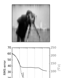
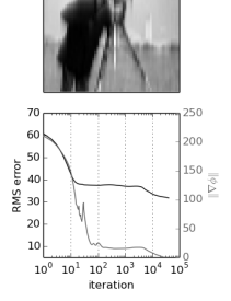
Figure 6: Gradient ascent performance using a randomly generated image sequence ($n=1000$ synthetic observations). The image (left) corresponds to the final estimate $\hat{x}_{t}$ after $t=10^{5}$ iterations. The plot (right) shows the RMS error curve of the estimate $\hat{x}_{t}$ as well as the norm of the gradient $\nabla\phi$.

4 Eigenvector method

So far, we have derived an optimization problem based on likelihood maximization, whose solution $\hat{x}$ recovers the undeteriorated image from its blurry and noisy observations. We have applied an iterative ascending method and found that the computation of $\hat{x}$, as we have formulated it so far, is difficult, due to the presence of local extrema in the objective function $\phi$. In this section, we study a different objective function, which is computationally easier to optimize. We will see, that – under specific conditions – this optimization problem is equivalent to the likelihood maximization-based method described in Section 3.

We start by rewriting Eq. (3.11) as the minimization of $-\sum_{i=1}^{m}\lambda_{i}u_{i}^{\mathsf{T}}\mathrm{P}_{X}u_{i}-\lambda_{i}u_{i}^{\mathsf{T}}u_{i}$, where the summands $-\lambda_{i}u_{i}^{\mathsf{T}}u_{i}$ may be added to the objective function without affecting the solution since they are constant w.r.t. $x$. This yields $\hat{x}=\arg\min_{x}\sum_{i=1}^{m}\lambda_{i}u_{i}^{\mathsf{T}}\left(I-\mathrm{P}_{X}\right)u_{i}$, where we recognize $\mathrm{P}_{X^{\perp}}=I-\mathrm{P}_{X}$ as the projector onto the orthogonal complement of the range of $X$ (see, e.g., [25]). Using the idempotency and symmetry of $\mathrm{P}_{X^{\perp}}$, we obtain

$$\hat{x}=\arg\min_{x}\varphi\left(x\right),\qquad\varphi\left(x\right)=\sum_{i=1}^{m}\lambda_{i}\left\|\mathrm{P}_{X^{\perp}}u_{i}\right\|^{2}\text{.}$$ (4.1)

In the following, we will consider three cases, which will be explained in more detail, when they come into play:

1. We start with the idealistic, noise-free case $m=N_{a}$.

2. We consider the still idealistic, noisy case $m=N_{a}$.

3. Finally, we study the realistic case $m<N_{a}$.

The case $m>N_{a}$ can only occur, if either $N_{a}$ is underestimated or $m$ is determined incorrectly. Then, revisiting $m$ or $N_{a}$ yields one of the other cases.

4.1 Noise-free $m=N_{a}$ case

Recall from Section 2 that in the noise-free case, any observation $y_{i}=Xa_{i}$ is a linear combination of the columns of the matrix $X=X\!\left(x_{\text{true}}\right)$, and thus $\operatorname{range}U\subseteq\operatorname{range}X$. This means that the minimum of the objective function $\varphi$ in Eq. (4.1) is $\varphi\left(\hat{x}\right)=0$. Since $m$ was defined in Section 2.3 so that $\lambda_{i}>0$ for all $i\leq m$, it is seen that $\varphi\left(x\right)=0$ can occur if and only if $\mathrm{P}_{X^{\perp}}u_{i}=0$ for all $i\leq m$. Thus, $\varphi\left(x\right)=0$ occurs not just if, but also only if $\operatorname{range}U\subseteq\operatorname{range}X$.

Consider the statement, that $\mathrm{P}_{U^{\perp}}x_{k}=0$ for all $k$, where the vectors $x_{1},\dots,x_{N_{a}}$ are the columns of the matrix $X=X\!\left(x\right)$ and thus span the range of $X$. Clearly, this statement is true if and only if $x$ is chosen so that $\operatorname{range}X\subseteq\operatorname{range}U$. The inclusion “$\subseteq$” tightens to the equality $\operatorname{range}U=\operatorname{range}X$ if $x=x_{\text{true}}$ and $m=N_{a}$, as it is seen from Eq. (2.7). Thus, for $m=N_{a}$ and in the absence of noise, we obtain the fundamental equivalence

$$\varphi\left(x\right)=0\enspace\Leftrightarrow\enspace\mathrm{P}_{U^{\perp}}x_{k}=0\enspace\forall k\text{.}$$ (4.2)

The eigenvalues $\lambda_{1},\dots,\lambda_{m}$ only appear in $\varphi$, but not on the right-hand side of the “$\Leftrightarrow$”.

The fundamental equivalence (4.2) means that, for $m=N_{a}$ and in the absence of noise, we can solve the original minimization problem (4.1) by instead minimizing the residuals $\left\|\mathrm{P}_{U^{\perp}}x_{k}\right\|\!{}^{2}$, i.e.

$$\hat{x}=\arg\min_{x}\sum_{k=1}^{N_{a}}\left\|\mathrm{P}_{U^{\perp}}x_{k}\right\|^{2}\enspace\text{s.t.}\enspace\hat{x}^{\mathsf{T}}\hat{x}=1\text{,}$$ (4.3)

where we add the constraint $\hat{x}^{\mathsf{T}}\hat{x}=\left\|\hat{x}\right\|=1$ to avoid the trivial solution $\hat{x}=0$. We are allowed to do this, because the optimization problems from Eq. (4.3) and (4.1) are solved by the same $x$, and as pointed out in Section 3.4, the value of the objective function is invariant to scalar factors.

To construct the vectors $x_{k}$, we define an $N_{y}\times N_{x}$ matrix $B_{k}$ so that $B_{k}x=b_{k}\ast_{\text{valid}}x$, where $b_{k}\in\mathbb{R}^{N_{a}}$ is the $k$-shifted Kronecker delta, i.e. with $b_{k}\!\left[i\right]=\left\{\text{$1$ if $k=i$; $0$ else}\right\}$ (see, e.g., [22]). Then, the linearity of convolution implies that $\operatorname{span}\left\{B_{k}x\middle|k\right\}=\operatorname{span}\left\{A_{i}x\middle|i\right\}$ for $m=N_{a}$. From the commutativity of convolution $A_{i}x=Xa_{i}$ we see in particular, that $x_{k}=B_{k}x$, and obtain

$$\hat{x}=\arg\min_{x}x^{\mathsf{T}}M\,x\enspace\text{s.t.}\enspace\hat{x}^{\mathsf{T}}\hat{x}=1,\qquad M=\sum_{k=1}^{N_{a}}B_{k}^{\mathsf{T}}\left(I-UU^{\mathsf{T}}\right)B_{k}\text{.}$$ (4.4)

Due to the constraint $\hat{x}^{\mathsf{T}}\hat{x}=1$, the objective function in Eq. (4.4) is recognized as the Rayleigh quotient $x^{\mathsf{T}}M\,x/x^{\mathsf{T}}x$. Since the matrix $M$ is symmetric, the Rayleigh-Ritz theorem [25] states that $\hat{x}$ is the eigenvector of $M$, which corresponds to its smallest eigenvalue. This eigenvalue is the value of the objective function for $x=\hat{x}$, that is $\varphi\left(\hat{x}\right)=0$. Since the matrix $M$ is positive semidefinite due to Eq. (4.3), all its eigenvalues are real and non-negative. There may be other eigenvectors for eigenvalue $0$, but not if the original optimization problem’s solution is unique up to a scalar factor.

4.2 Noisy $m=N_{a}$ case

In the previous section, we have seen that the objective function $\sum_{k=1}^{N_{a}}\left\|\mathrm{P}_{U^{\perp}}x_{k}\right\|^{2}$ of Eq. (4.3) is $0$, if and only if all columns $x_{1},\dots,x_{N_{a}}$ of the matrix $X=X\!\left(x_{\text{true}}\right)$, can be represented as linear combinations of the eigenvectors $u_{1},\dots,u_{m}$. We express such a linear combination as $x_{k}=Uc_{k}$ with a weighting vector $c_{k}$, where $c_{k}\!\left[i\right]$ corresponds to the contribution of $u_{i}$ to $x_{k}$.

It was shown in Section 2.3 that for higher noise levels (and a small number $n$ of images), the signal subspace is reflected less truthfully and the eigenvectors encoded in the matrix $U$ become misaligned. Although this error can be kept small by increasing the number $n$ of observations, in practical applications, at least a small error $\rho_{i}$ always remains on every eigenvector $u_{i}$, since the number of observations must be finite. Looking close at the eigenvectors shown in Figure 4b–4d, one can see that this error appears as “noisy” grain. We will quantify the error as $\rho_{i}\sim\mathcal{N}\left(0;\Sigma_{i}\right)$ without assuming that $\rho_{i}$ is i.i.d., because this would disrespect the orthonormal nature of the eigenvectors $u_{1},\dots,u_{m}$.

In general, a vector $c_{k}$ which satisfies $x_{k}=Uc_{k}$ for $x=x_{\text{true}}$ does not necessarily exists for all $k$ when the columns of $U$ are misaligned due to noise. Still, it does exist for $x_{k}=\left[u_{1}-\rho_{1}\,\dots\,u_{m}-\rho_{m}\right]c_{k}$, where $u_{i}-\rho_{i}$ are the unknown, error-free eigenvectors. By rewriting $\left[u_{1}-\rho_{1}\,\dots\,u_{m}-\rho_{m}\right]c_{k}$ as $Uc_{k}-\sum_{i=1}^{m}c_{k}\!\left[i\right]\rho_{i}$, we see that

$$x_{k}=Uc_{k}-\delta_{k}\text{,}$$ (4.5)

where $\delta_{k}=\sum_{i=1}^{m}c_{k}\!\left[i\right]\rho_{i}$ is the normal-distributed, zero-mean residual with

$$\operatorname{Cov}\delta_{k}=\sum_{i=1}^{m}\Sigma_{i}c_{k}\!\left[i\right]^{2}\text{.}$$ (4.6)

If the errors $\rho_{1},\dots,\rho_{m}$ of the eigenvectors $u_{1},\dots,u_{m}$ do not occur to be linear combinations of the eigenvectors, i.e. $\rho_{i}\not\in\operatorname{range}U$ for all $i=1,\dots,m$, then we get $\delta_{k}\not\in\operatorname{range}U$, since $\delta_{k}$ is a linear combination of the errors. We also get $\delta_{k}\not\in\operatorname{range}U$ if only some errors $\rho_{i}$ are not in the range of $U$, as long as these $\rho_{i}$ are not zero-weighted by $c_{k}$. According to Eq. (4.5), we can write the objective function as $\sum_{k=1}^{N_{a}}\left\|\mathrm{P}_{U^{\perp}}x_{k}\right\|\!{}^{2}=\sum_{k=1}^{N_{a}}\left\|\mathrm{P}_{U^{\perp}}\delta_{k}\right\|\!{}^{2}$, because $\mathrm{P}_{U^{\perp}}Uc_{k}=0$. Consequently, when the noise level rises and the eigenvector errors $\rho_{i}$ grow, the value of the objective function for $x=x_{\text{true}}$ becomes greater than $0$.

Since choosing $x=\hat{x}$ minimizes $\sum_{k=1}^{N_{a}}\left\|\mathrm{P}_{U^{\perp}}x_{k}\right\|^{2}\stackrel{{\scriptstyle\hbox to0.0pt{\eqref{eq:method_noisy_residual}\hss}}}{{=}}\sum_{k=1}^{N_{a}}\left\|\mathrm{P}_{U^{\perp}}\delta_{k}\right\|^{2}$ by definition, the covariances $\operatorname{Cov}\delta_{k}$ of the residuals are also minimized. Due to Eq. (4.6), this induces a preference for those $c_{k}$ which assign a small weight $c_{k}\!\left[i\right]$ for $\Sigma_{i}$ if $\Sigma_{i}$ is large. This means that $c_{k}$ tends to weight the columns of $U$ in accordance to their reliability, and the most reliable eigenvector is $u_{1}$ (see Section 2.3.2). Therefore, when the noise level is increased, the contribution from $u_{1}$ tends to be overestimated – which makes $\hat{x}$ become more blurry, but not noisier than $u_{1}$. Surprisingly, this mechanism works without taking the eigenvalues $\lambda_{1},\dots,\lambda_{m}$ into account, which encode the reliability of the corresponding $u_{i}$. Inventing a mechanism to counter-balance the overestimation remains an open problem for future research.

4.3 Noisy $m<N_{a}$ case

So far, we have confined ourselves to the case $m=N_{a}$ which yields the equality $\operatorname{range}U=\operatorname{range}X$ for $X=X\!\left(x_{\text{true}}\right)$. We have seen, how this can be utilized to minimize $\sum_{k=1}^{N_{a}}\left\|\mathrm{P}_{U^{\perp}}x_{k}\right\|\!{}^{2}$ instead of $\sum_{i=1}^{m}\left\|\mathrm{P}_{X^{\perp}}u_{i}\right\|\!{}^{2}$. But as we already mentioned in Section 2.2, the assumption $m=N_{a}$ is rarely true in practice, so the strict inclusion $\operatorname{range}U\subset\operatorname{range}X$ is a rather realistic condition for $X=X\!\left(x_{\text{true}}\right)$. The fundamental equivalence (4.2) does not hold then.

The case $m<N_{a}$ can always be seen as the situation that an insufficient amount of observations was acquired. As we described in Section 2.3, the signal subspace dimension $m$ equals the dimension of the PSF subspace $\operatorname{span}\left\{a_{1},\dots,a_{n}\right\}$ if $x_{\text{true}}$ is persistently exciting. Thus, encountering $m<N_{a}$ means that the observations were generated from PSFs which did not contain enough variance. Acquiring additional observations generated from the “missing” PSFs would establish the $m=N_{a}$ case. To some extent, such acquisition can be synthesized, as described below.

4.3.1 Inflating the observations

The rule of associativity in Eq. (2.5) allows us to artificially generate additional observations with unobserved PSFs. To accomplish this, we transform each observation $y_{i}$ using a valid convolution matrix $D_{t}$, whose underlying filter is a $t$-shifted Kronecker delta, i.e. with $d_{t}\!\left[i\right]=\left\{\text{$1$ if $t=i$; $0$ else}\right\}$ of size $N_{d}$ (see, e.g., [22]). According to Eq. (2.7),

$$D_{t}y_{i}\stackrel{{\scriptstyle\hbox to0.0pt{\eqref{eq:convolution:associativity}\hss}}}{{=}}\left(d_{t}\ast_{\text{full}}a_{i}\right)\ast_{\text{valid}}x_{\text{true}}+D_{t}\varepsilon_{i}$$ (4.7)

shifts the PSF $a_{i}$, which generated the observation $y_{i}$, by the offset of the Kronecker delta. By inflating we mean the substitution of the original observations by $D_{1}Y,\dots,D_{N_{d}}Y$. However, inflating not only increases the signal subspace dimension $m$, but, due to full convolution, also increases the dimension of the PSFs (see Section 2.1). Below, $m$, $N_{a}$, and $N_{y}$ refers to the respective quantities after inflating, and, to avoid confusion, we will write $m_{0}$, $N_{a,0}$, and $N_{y,0}$ to refer to the original quantities.

Figure 7 shows the typical behavior of $N_{a}$ and $m$ after inflating in dependence of the filter size $N_{d}$ for randomly generated, $m_{0}$-dimensional PSFs with $m_{0}<N_{a,0}$. The signal subspace dimension $m$ was estimated as the rank of the matrix $Y$. As can be seen from comparison of Figure 7a and Figure 7b, an initially greater signal subspace dimension $m_{0}$ facilitates, that smaller filter sizes $N_{d}$ suffice for reaching the desired $m=N_{a}$ state (for fixed $N_{a,0}$).

(a) $m_{0}=5$

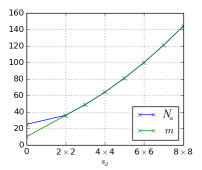
(b) $m_{0}=10$

Figure 7: The plots show how the PSF dimension $N_{a}$ and the signal subspace dimension $m$ typically grow, when each observation $y_{i}$ is inflated according to Eq. (4.7) using different sizes $N_{d}$ of the inflating filter $d_{t}$ (horizontal axes). The original PSFs were $N_{a,0}=5\times 5$ pixels in size and sampled from a random, $m_{0}$-dimensional subspace of $\mathbb{R}^{N_{a,0}}$. The plots were computed using $n=10{,}000$ noisy observations of the ground truth in Figure 1a, sampled down to $N_{x}=32\times 32$ pixels, with $\varepsilon_{i}\sim\mathcal{N}\left(0;I\cdot 10^{-1}\right)$.

4.3.2 When inflating is not enough

Depending on the PSF subspace, it might be that the $m=N_{a}$ state cannot be reached by inflating (e.g., for PSFs with disk-shaped support). Generally, the more pixels at the corners of all observed PSFs are constant, the greater the gap of $m$ and $N_{a}$ will remain after inflating. This can be tackled by reducing $N_{a}$ in the one-dimensional case.

For images, we leave out those columns $x_{k}$ of the matrix $X$, which do not appear in the range of $U$, so that that the fundamental equivalence (4.2) holds for $X=X\!\left(x_{\text{true}}\right)$. To do this, we introduce the matrix

$$M_{\ast}=Q\!\left(h\right)+\alpha\cdot\sum_{k=1}^{N_{a}}h\!\left[k\right]\cdot M_{k},\qquad\text{where }M_{k}=B_{k}^{\mathsf{T}}\left(I-UU^{\mathsf{T}}\right)B_{k}\text{,}$$ (4.8)

which generalizes the matrix $M$ from Section 4.1. Let $Q\!\left(h\right)=0$ and $\alpha=1$ for simplicity first. If the $N_{a}$-shaped vector $h$, called the PSF footprint, suffices

$$h\left[k\right]=\begin{cases}0&\text{if }a_{i}\left[k\right]=0\text{ for all }i,\\ 1&\text{else,}\end{cases}$$ (4.9)

then $M_{\ast}\,x_{\text{true}}\xrightarrow{n\to\infty}0$. Yet, the minimization of $x^{\mathsf{T}}M_{\ast}\,x$ w.r.t. $x$ does not necessarily recover $x_{\text{true}}$, as the following example illustrates: Given that $a_{i}\left[1\right]=0$ for all $i$ and $h=\left(0,1,\dots,1\right)$, the vector $\delta_{N_{x}}=\left(0,\dots,0,1\right)$ also yields $M_{\ast}\,\delta_{N_{x}}=0$. This is because no information about the last pixel was observed.

Fortunately, the knowledge of the PSF footprint $h$ makes the solution of this ambiguity straight-forward, by choosing

$$Q\!\left(h\right)=\operatorname{Diag}q\!\left(h\right),\qquad\text{where }q\!\left(h\right)=1_{N_{x}}-\min\left\{1_{N_{x}},\ h\ast_{\text{full}}1_{N_{y}}\right\}\text{.}$$ (4.10)

Then, $x^{\mathsf{T}}Q\,x$ produces high responses for $x$ with non-zero values in those pixels, for which no information was observed. The minimization of $x^{\mathsf{T}}M_{\ast}\,x$ w.r.t. $x$ in accordance with Eq. (4.8) and (4.10) forces these pixels to $0$, and if $h$ and $U$ are accurate so that $m=\left\langle 1,h\right\rangle$, then the minimization

$$\hat{x}_{\ast}=\arg\min_{x}x^{\mathsf{T}}M_{\ast}\,x\enspace\text{s.t.}\enspace x^{\mathsf{T}}x=1$$ (4.11)

yields the generalized estimate $\hat{x}_{\ast}$ which recovers the ground truth $x_{\text{true}}$. Note that the condition $m=\left\langle 1,h\right\rangle$ is a generalization of $m=N_{a}$ to the case that the PSF footprint $h$ may have $0$-entries, where $\left\langle\cdot,\cdot\right\rangle$ denotes the inner product.

4.3.3 Estimating the PSF footprint

So far, we have described a solution of the MFBD problem based on the computation of the eigenvector of a specifically constructed matrix $M_{\ast}$. The only ingredient of this matrix, which remains unspecified, is the PSF footprint $h$. We propose determining the footprint $h$ heuristically by alternating minimization of $\hat{x}^{\mathsf{T}}M_{k}\,\hat{x}$ w.r.t. $\hat{x}$ and $h$. Note that this is different from alternating optimization w.r.t. the undeteriorated image $x$ and the filters $a_{1},\dots,a_{n}$, since only one footprint needs to be determined for the whole image sequence.

The procedure is outlined in Algorithm 1, which only takes the model parameter $N_{a}$ and the truncated matrix of eigenvectors $U$ of the covariance matrix of the observations as input. The initialization of $\hat{x}_{\ast}$ using a rough estimate and the iterative refinement are described in Section 4.4.1 and Section 4.4.2 below.

Input: $N_{a}$ and the truncated matrix of eigenvectors $U=\left(u_{1},\dots,u_{m}\right)$ of the covariance matrix of the observations

Output: the generalized estimate $\hat{x}_{\ast}$ and the estimated PSF footprint $h$

initialize $h$ as a vector of size $N_{a}$ with all entries set to $1$;

initialize $\hat{x}_{\ast}$ using a rough estimate;

repeat

       $R\left[k\right]\leftarrow\hat{x}_{\ast}^{\mathsf{T}}M_{\ast}\,\hat{x}_{\ast}$ for all $k$;

       update $h\!\left[k\right]\leftarrow 0$ where $R\left[k\right]$ is largest;

       refine the estimate $\hat{x}_{\ast}$ using the updated footprint $h$;

      

until $m=\left\langle 1,h\right\rangle$;

Algorithm 1 Outline of the computation of the generalized estimate $\hat{x}_{\ast}$ from an unknown PSF footprint $h$.

4.4 Implementation

The first step to the computation of the estimate $\hat{x}_{\ast}$ is the identification of the signal subspace, i.e. $\operatorname{range}U$, as described in Section 2.3.2. Instead of computing the EVD of the $N_{y}\times N_{y}$ empirical covariance matrix $\frac{1}{n}YY^{\mathsf{T}}=U\Lambda U^{\mathsf{T}}$, that is too large to be kept in memory for high-resolution images, we rely on the truncated singular value decomposition (SVD, see, e.g., [23]) of $Y=VSW^{\mathsf{T}}$ with $S=\operatorname{Diag}\left(s_{1},\dots,s_{N_{a}}\right)$ and $s_{i}\geq s_{i+1}$. We only compute the $N_{a}$ largest singular values $s_{i}$. Since $\frac{1}{n}YY^{\mathsf{T}}=\frac{1}{n}VSW^{\mathsf{T}}WSV^{\mathsf{T}}=\frac{1}{n}VS^{2}V^{\mathsf{T}}$, the SVD of $Y$ recovers the eigenvectors $U=V$ of the covariance matrix with corresponding eigenvalues $\lambda_{i}=s_{i}^{2}/n$.

The SVD implementations which we have considered are shown in Table 1. The “_getsdd” routine from LAPACK produces accurate results, but demands that the entire matrix $Y$ is loaded into memory. As the matrix $Y$ becomes too large, we must access it in portions from a slower storage. Halko et al. [26] proposed two SVD implementations with a memory complexity of $\mathcal{O}\left(N_{y}\cdot\left(N_{a}+\kappa\right)\right)$, where a greater $\kappa$ increases noise robustness:

Single-pass SVD:

The single-pass SVD processes the columns of the matrix $Y$ one-by-one in a streaming fashion. On the downside, the implementation has proven to become inaccurate in the presence of noise.

Randomized SVD:

The randomized SVD is not designed for off-memory data specifically. Nevertheless, it can be easily adapted for this use-case, since it accesses the matrix $Y$ solely within dot products. With a block-wise dot product implementation, this implementation outperforms the other two in terms of speed at lower resolutions, if the blocks are chosen at least the size of $N_{y}$ elements.

To determine the best suited implementation, we have performed a quantitative comparison of the computation time required by the different implementations. The results are shown in Table 2.

Table 1: Qualitative comparison of SVD implementations, based on their memory complexity and noise robustness.

Data size	$\sigma^{2}/n$ ratio	Suited SVD routine
Small	Any	LAPACK’s “_gesdd”
Any	Small	Single-pass SVD
Moderate/high	Moderate/high	Randomized SVD

Table 2: Quantitative comparison of the computation time different SVD implementations on regular consumer hardware. LAPACK was not applicable to very large image data (“—”). The results are reported in seconds and the best results are highlighted.

	$n=500$				$n=4000$
	$N_{y}=10^{2}$	$N_{y}=10^{3}$	$N_{y}=10^{4}$	$N_{y}=10^{5}$	$N_{y}=10^{2}$	$N_{y}=10^{3}$	$N_{y}=10^{4}$	$N_{y}=10^{5}$
Randomized SVD:	$0.011$	$0.083$	$1.007$	$23.523$	$0.076$	$0.577$	$6.977$	$182.782$
Single-pass SVD:	$0.033$	$0.112$	$1.000$	$11.481$	$0.212$	$0.689$	$4.809$	$63.131$
LAPACK:	$0.016$	$1.858$	$14.314$	—	$0.117$	$23.534$	—	—

For efficient implementation of the inflating method described in Section 4.3.1, computation of the potentially huge $N_{y}\times nN_{d}$ matrix $\left(D_{1}Y,\dots,D_{N_{d}}Y\right)$ should be avoided. The SVD of $Y=USW^{\mathsf{T}}$ shows that

$$\operatorname{range}D_{t}Y=\operatorname{range}D_{t}US\text{,}$$ (4.12)

since $W^{\mathsf{T}}$ has full column rank. Thus, inflating can be performed efficiently by computing the smaller $N_{y}\times m_{0}N_{d}$ matrix $\left[D_{1}US\,\dots\,D_{N_{d}}US\right]$, which comes at the cost of an additional SVD. Throughout the results we present in Section 4.5, we used the LAPACK implementation for the second SVD.

4.4.1 Rayleigh quotient iterations

Algorithm 1 requires the computation of the estimate $\hat{x}_{\ast}$ for initialization. Given a roughly known eigenvalue $\mu_{0}$ of the matrix $M_{\ast}$, the corresponding eigenvector $\hat{x}_{\ast}$ can be computed using Rayleigh quotient iterations,

$$\left(M_{\ast}-\mu_{k}I\right)\hat{x}_{\ast,k+1}=\hat{x}_{\ast,k},$$ (4.13)

where $\mu_{k}=\hat{x}_{\ast,k}^{\mathsf{T}}\,M_{\ast}\,\hat{x}_{\ast,k}$ for $k\geq 1$. In each iteration, the linear system in Eq. (4.13) is solved for $\hat{x}_{\ast,k+1}$ and then normalized. The convergence rate of the iterations is cubic (e.g., [27]). The choice of $\hat{x}_{\ast,0}$ is random.

Since the eigenvector $\hat{x}_{\ast}$ corresponds to the eigenvalue of $M_{\ast}$ which is closest to $0$, choosing $\mu_{0}=0$ is reasonable. We used Newton iterations with Krylov approximation of the inverse Jacobian [28] for the solution of the linear system.

Algorithm 2 summarizes the approximation of $\hat{x}_{\ast}$ to a given precision, which is estimated based upon the convergence of the $\mu_{k}$ sequence. It is convenient to set the parameter $\alpha$ in Eq. (4.8) to $\alpha=1/N_{a}$, so $\mu_{k}$ becomes independent of $N_{a}$. The bottleneck of the algorithm is the solution of the linear system in Eq. (4.13). However, due to the cubic convergence rate of the algorithm, high precisions are reached after only few iterations.

Input: the matrix $M_{\ast}$ and the required precision $1/\mu_{\Delta}$

Output: the estimate $\hat{x}_{\ast}$

initialize $\mu^{\prime}\leftarrow 0$ and $\hat{x}_{\ast}$ randomly;

repeat

       $\mu\leftarrow\mu^{\prime}$;

       $\hat{x}_{\ast}\leftarrow\text{solve }\left(M_{\ast}-\mu I\right)\hat{x}^{\prime}_{\ast}=\hat{x}_{\ast}\text{ for }\hat{x}^{\prime}_{\ast}$;

       $\hat{x}_{\ast}\leftarrow\hat{x}_{\ast}/\hat{x}_{\ast}^{\mathsf{T}}\hat{x}_{\ast}$;

       $\mu^{\prime}\leftarrow\hat{x}_{\ast}^{\mathsf{T}}M_{\ast}\,\hat{x}_{\ast}$;

      

until $\left|\mu^{\prime}-\mu\right|<\mu_{\Delta}$;

Algorithm 2 Computation of the generalized estimate $\hat{x}_{\ast}$ using Rayleigh quotient iterations.

We have used used $\mu_{\Delta}=10^{-3}$ for Algorithm 2 in all our experiments.

4.4.2 Estimate refinements

Recall that besides of computing the estimate $\hat{x}_{\ast}$ for initialization, Algorithm 1 also relies on incremental updating of the estimate. We found that rather rough refinements are sufficient, which can be performed faster than using a single iteration of Algorithm 2, as described below.

In Section 4.1 we argued that the matrix $M$ is symmetric and positive semidefinite, and so are the matrices $Q\!\left(h\right)$ and $M_{\ast}$ in Eq. (4.8). Let $\mu_{\text{up}}$ be an upper bound of the eigenvalues of the matrix $M_{\ast}$ and let $\mu_{\text{min}}$ be the smallest eigenvalue. We define the spectrum-shifted matrix $Z=\mu_{\text{up}}I-M_{\ast}$ and observe that $Z\hat{x}_{\ast}=\mu_{\text{up}}\hat{x}_{\ast}-\mu_{\text{min}}\hat{x}_{\ast}$, so $\hat{x}_{\ast}$ is an eigenvector of matrix $Z$ with eigenvalue $\mu_{\text{up}}-\mu_{\text{min}}$, which also is the largest eigenvalue of the matrix $Z$.

For $k\to\infty$, the power iterations $\hat{x}_{\ast,k+1}=Z\hat{x}_{\ast,k}$ recover the eigenvector $\hat{x}_{\ast}$ of the matrix $Z$ corresponding to the largest eigenvalue of $Z$ (see, e.g., [27]). For the upper bound $\mu_{\text{up}}$ of the eigenvalues of the matrix $M_{\ast}$ we used $\mu_{\text{up}}=1+\alpha N_{a}$, which is legitimate due to the following two reasons:

1. The largest eigenvalue of matrix $M_{k}$ in Eq. (4.8) is $1$, the matrix since $B_{k}$ contains at most a single $1$ in each of column, and $I-UU^{\mathsf{T}}$ is a projection matrix.

2. The matrix $Q\left(h\right)$ is a binary diagonal matrix, with eigenvalues $0$ and $1$.

Algorithm 3 summarizes the resulting procedure for the refinement of the estimate $\hat{x}$.

Input: $N_{a}$, the matrix $M_{\ast}$, an initial estimate $\hat{x}_{\ast}$, and the required precision $1/\mu_{\Delta}$

Output: the refined estimate $\hat{x}_{\ast}$

define $Z\leftarrow\left(1+\alpha N_{a}\right)I-M_{\ast}$;

initialize $\mu\leftarrow\hat{x}_{\ast}^{\mathsf{T}}Z\,\hat{x}_{\ast}$ and $w\leftarrow\hat{x}$;

repeat

       $\mu^{\prime}\leftarrow\mu$;

       $\hat{x}_{\ast}\leftarrow w/w^{\mathsf{T}}w$;

       $w\leftarrow Z\hat{x}_{\ast}$;

       $\mu\leftarrow x_{\ast}^{\mathsf{T}}w$;

      

until $\left|\mu^{\prime}-\mu\right|<\mu_{\Delta}$;

Algorithm 3 Refinement of the generalized estimate $\hat{x}_{\ast}$ using power iterations.

We have used used $\mu_{\Delta}=10^{-4}$ for Algorithm 3 in all our experiments.

4.4.3 Further optimizations

Instead of using Algorithm 1 to jointly compute the generalized estimate $\hat{x}_{\ast}$ and the PSF footprint, a two-step scheme is more efficient. In the first step, the algorithm is used for only a small image section of the observations to compute the PSF footprint. In our experiments, using image sections of width and height $3$ to $8$ times larger than $N_{a}$ offered a good trade-off between reliability and speed. In the second step, $\hat{x}_{\ast}$ is computed directly using Algorithm 2 and the already determined PSF footprint.

Algorithm 1, 2, and 3 require the $N_{x}\times N_{x}$ matrix $M_{\ast}$ as input. However, since this matrix only appears within dot products, there is no need to compute its explicit representation. We rewrite the linear system $\left(M_{\ast}-\mu I\right)\hat{x}_{\ast}^{\prime}=\hat{x}_{\ast}$ in Algorithm 2 as $M_{\ast}\hat{x}_{\ast}^{\prime}-\mu\hat{x}_{\ast}^{\prime}-\hat{x}_{\ast}=0$ for this purpose. Therefore, the memory complexity of the three algorithms is not larger than $\mathcal{O}\left(N_{x}+mN_{y}\right)$.

The computation of dot products with the matrix $M_{\ast}$ is a very frequent operation, which is worth to be implemented for maximum efficiency. To this end, we implemented the matrix-vector-product $B_{k}x$ in Eq. (4.8) as image cropping, and $B_{k}^{\mathsf{T}}y$ as image padding operations. Depending on the implementation of the linear algebra, the batched computation of

$$UU^{\mathsf{T}}\left(\dots,B_{k}x,\dots\right)$$ (4.14)

may be faster than the sequential

$$\dots,UU^{\mathsf{T}}B_{k}x,\dots\text{,}$$ (4.15)

as it allows to exploit memory localities. In our Python-based implementation, this optimization accelerated the dot product computations by up to factor $7$. Furthermore, it is appropriate to evaluate the batches in parallel.

For post-processing, we scaled $\hat{x}_{\ast}$ by a factor determined as the mean pixel value of the observations.

4.5 Experimental results

In this section, we describe the application of our eigenvector-based method to synthetically generated image sequences. The pixel values were of all images were restricted to the interval $\left[0,255\right]$. All experiments were performed using dated consumer hardware, comprising only 4 GiB RAM and an Intel Core i5-3320M CPU. In addition, we have also included a quantitative comparison of our method to [20].

For quantitative evaluation of the results, we use the norm-invariant root mean square (RMS) error,

$$\frac{1}{\sqrt{N_{x}}}\cdot\left\|x_{\text{true}}-\frac{\left\|x_{\text{true}}\right\|}{\left\|x\right\|}\cdot x\right\|_{\mathsf{Fro}},$$ (4.16)

which is invariant to the norm of the result image $\hat{x}_{\ast}$. We ignore those pixels of $\hat{x}_{\ast}$ and $x_{\text{true}}$, which were not observed due to the generated PSFs (cf. Section 4.3.2).

4.5.1 Moderate noise levels

In a first experiment, we have used image sequences comprising $n=1000$ images, each sequence generated using an individual noise level $\sigma^{2}\in\left\{0.1,1,10\right\}$. The images were generated according to Eq. (2.7) using the ground truth image from Figure 1a of size $N_{x}=128\times 128$ pixels and random PSFs of size $N_{a,0}=10\times 10$ pixels, while only varying the $57$ pixels of the PSF footprint shown in Figure 8a. Example images from the three sequences are shown in Figure 8b–8d.

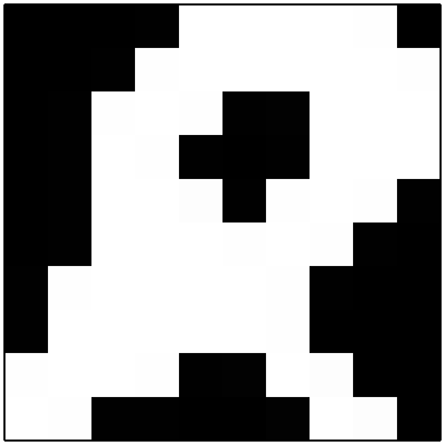
(a) PSF footprint

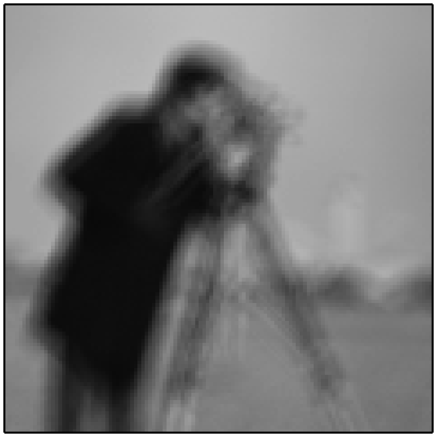
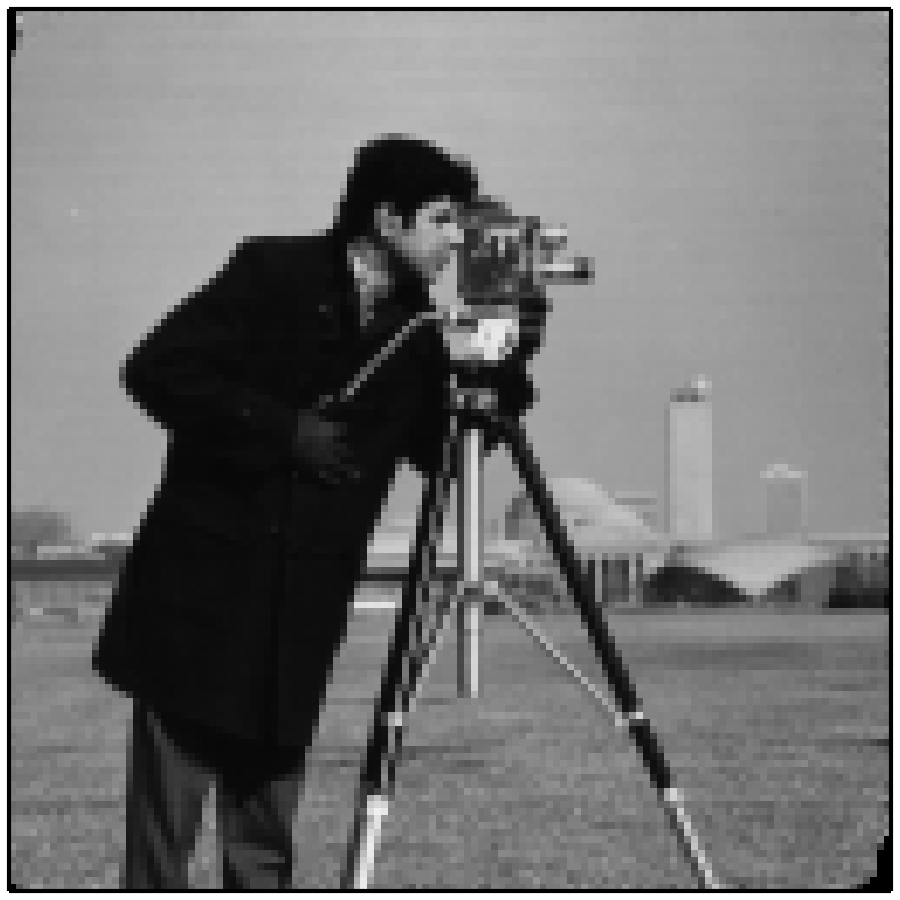
(b) $\sigma^{2}=10^{-1}$

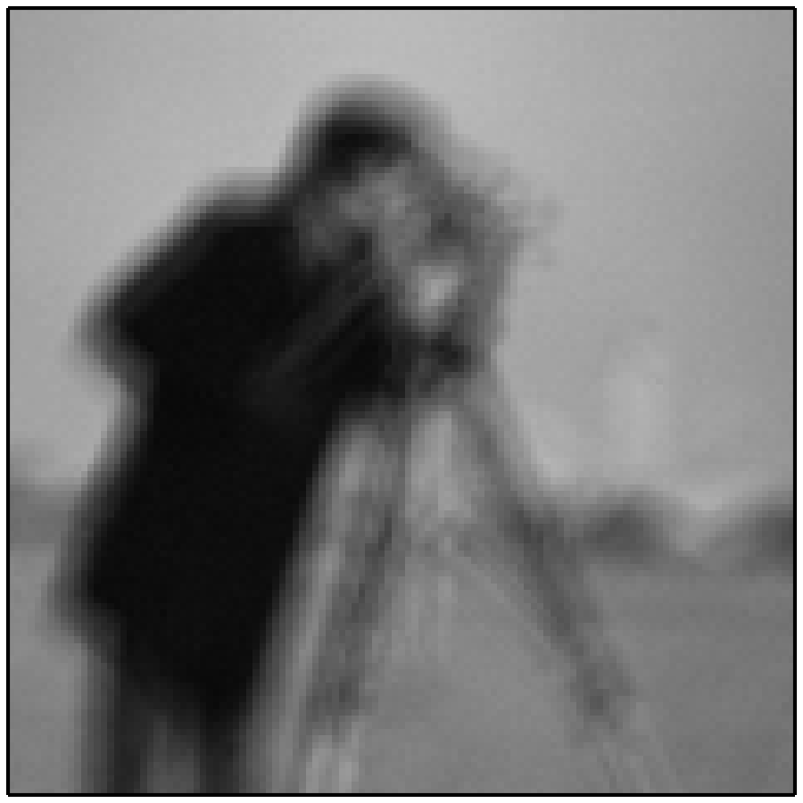
(c) $\sigma^{2}=10^{0}$

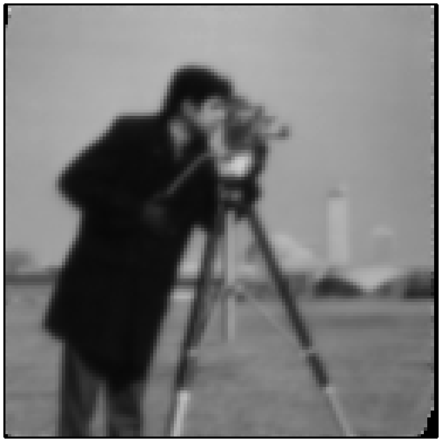
(d) $\sigma^{2}=10^{1}$

Figure 8: (a) $10\times 10$ pixels PSF footprint, where black pixels correspond to 0 and white pixels correspond to 1, and (first row) synthetically generated example observations, generated using the PSF footprint at different noise levels (b)–(d). (second row) The corresponding results obtained using the proposed eigenvector-based MFBD method.

The first step of our method is the recovery of the matrix $U$ which represents the signal subspace. For the lower noise levels $\sigma^{2}=0.1$ and $\sigma^{2}=1$, we have used the randomized SVD [26] to compute the EVD of the covariance matrix $\frac{1}{n}YY^{\mathsf{T}}$. In this experiment, we know that the dimension of the PSF subspace is equal to the number of the 1-entries in the PSF footprint, thus we skip inflating and proceed to the estimation of the PSF footprint directly. Using centered image sections of the size $N_{y}^{\prime}=75\times 75$ pixels, we exactly recovered the PSF footprint as described in Section 4.4.3.

The case correpsonding to the increased noise level $\sigma^{2}=10$ is more challenging. Since the obtained matrix representation of the signal subspace of the signal subspace is less accurate, the estimation of the PSF footprint yields inaccurate results. Fortunately, inflating the observations turns out being helpful. The reason is that, in contrast to the estimation of the PSF footprint, inflating reduces the gap between the signal subspace dimension $m$ and $N_{a}$ in a non-heuristic manner. We then estimated the PSF footprint from centered image sections of the size $N_{y}^{\prime}=38\times 38$ pixels of the inflated observations.

The final step of our method concerns the computation of the estimate $\hat{x}_{\ast}$ using the priorly estimated PSF footprint. The results are shown in the bottom row of Figure 8. For $\sigma^{2}=0.1$, the undeteriorated image is recovered almost perfectly up to the unobserved pixels in the upper left und lower right corners of the image (RMS value of 2.63). The result is somewhat blurrier for $\sigma^{2}=1$ (RMS value of 5.05). The result obtained for $\sigma^{2}=10$ is even blurrier (RMS value of 9.97 and 17.69 without inflating). This could be improved by taking more observations into account. In all three cases, the overall runtime of our method was about 1 minute without inflating, and increased to about 3 minutes using the inflated observations.

4.5.2 High noise levels

Our method specifically addresses the case of very high noise levels and large numbers of observations $n$. Thus, in a second experiment, we have used a larger image sequence comprising $n=5000$ images, which was generated using the noise level $\sigma^{2}=50$. We also reduced the ground truth size to $N_{x}=40\times 40$ pixels and used PSFs of the smaller size $N_{a}=5\times 5$ pixels. Figure 9a shows an example image from the sequence.

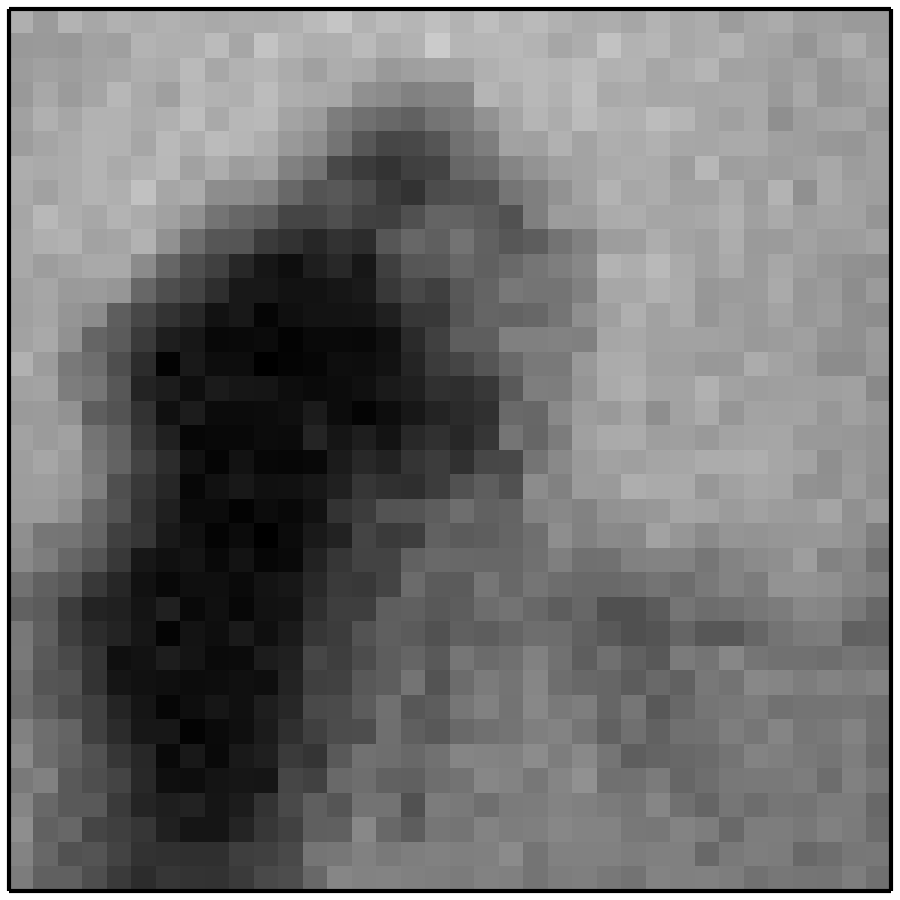
(a)

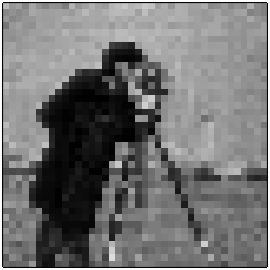
(b)

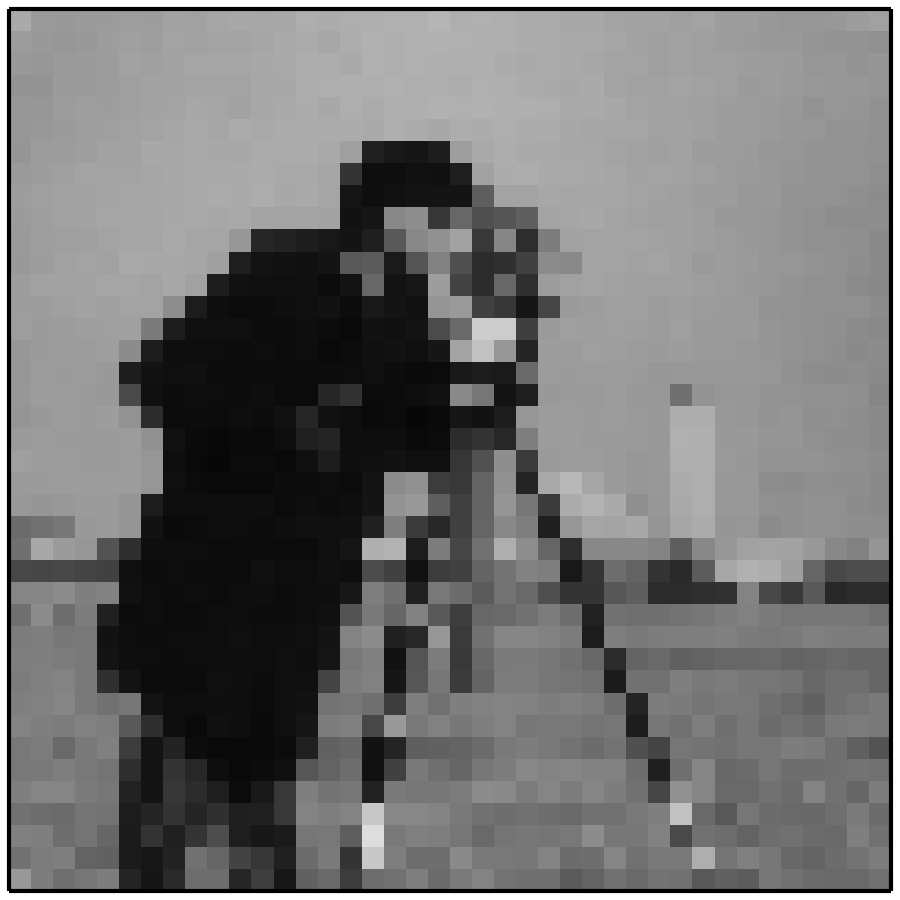
(c)

Figure 9: (a) Example observation generated using the high noise level $\sigma^{2}=50$, (b) result obtained using [20], and (c) result obtained using the proposed eigenvector-based MFBD method.

In Section 1.3, we described that other methods like [18] and [19] are intractable for this case due to the large size of the involved matrices. For example, the latter demands computation of a matrix of about 24 GiB using single-precision floating point numbers. For this reason, we compare our method against the online method [20]. However, this method is originally based on circular convolution. We found that, if implemented using valid convolution instead, the online method fails to converge if $m<N_{a}$. We thus used $m=N_{a}$ to generate the image sequence for this experiment. The result obtained using the online method yields an RMS value of 7.58. The method took 245 seconds to process the whole image sequence.

For our method, we again used the randomized SVD [26] for the recovery of the signal subspace, which terminated after $8.7$ seconds. Due to $m=N_{a}$, neither inflating needs to be performed, nor do we need to estimate the PSF footprint. The subsequent computation of the estimate $\hat{x}$ using Algorithm 2 took $0.5$ seconds. Both steps took only $9.3$ seconds in total and the obtained result yields an RMS value of 5.67. For comparison, we also computed the result obtained using the online method after $9.3$ seconds, which corresponds to an RMS value of 12.49. The results are shown in Figure 9b–9c. It can be seen that the result obtained using our method is minorly sharper than the result obtained using [20] and far less noisy.

Overall, our method yields a significantly improved result using the same computation time (RMS value of 12.49 compared to 5.67), and also an improved result if the online method is given more computation time (RMS value of 7.58 compared to 5.67).

5 Conclusions and future work

We have presented two methods for multi-frame blind deconvolution method, which recover an undeteriorated image from a sequence of its blurry and noisy observations. This is accomplished by exploiting the signal subspace, which is encoded in the empirical covariance matrix of the observations. The first presented method is based on likelihood maximization and requires careful initialization to cope with the non-convexity of the loss function. The second presented method circumvents this requirement by exploiting that, under two specific conditions, the same solution also emerges as an eigenvector of a specifically constructed matrix. The matrix is fully determined solely by the observations, so the filters corresponding to the observations do not need to be estimated, so alternating optimization schemes are not required. We have applied the eigenvector method to synthetically generated image sequences and performed a quantitative comparison with a previous method, obtaining strongly improved results.

The first condition demands that the number of observations is sufficiently large, so that the signal subspace of the noisy observations approximates the signal subspace of the unobservable, noise-free observations. The second condition demands that the dimension of the signal subspace is sufficiently large. To cope with this, we have described a pre-processing step which inflates the signal subspace by artificially generating additional observations. In addition, we have proposed an extension of the eigenvector method which copes with insufficient dimensions of the signal subspace by estimating a footprint of the unknown filters using an alternating optimization scheme.

Application of the proposed methods to a large variety of image data will be subject of future work. This will particularly comprise high-resolution and real-world images, as well as a more comprehensive evaluation, including more previous methods for comparison. Stable implementations of the proposed methods should automatically choose the best-suited method for computation of the SVD. Interesting open research questions were also pointed out in Section 4.2.

References

- Brown and Lowe [2007] Matthew Brown and David G Lowe. Automatic panoramic image stitching using invariant features. International Journal of Computer Vision, 74(1):59–73, 2007.
- Kostrykin et al. [2021] Leonid Kostrykin, Claus Rohr, and Karl Rohr. Globally optimal and scalable video image stitching for robotic inspection of electric generators. In Proc. International Conference on Control, Automation and Systems (ICCAS 2021), pages pp. 1141–1145, 2021.
- Gui and Li [2020] Zhongcheng Gui and Haifeng Li. Automated defect detection and visualization for the robotic airport runway inspection. IEEE Access, 8:76100–76107, 2020.
- Yang et al. [2019] Liang Yang, Bing Li, Guoyong Yang, Yong Chang, Zhaoming Liu, Biao Jiang, and Jizhong Xiaol. Deep neural network based visual inspection with 3D metric measurement of concrete defects using wall-climbing robot. In Proc. International Conference on Intelligent Robots and Systems (IROS), pages 2849–2854, 2019.
- Ramaswamy et al. [2018] Akshaya Ramaswamy, Jayavardhana Gubbi, Rishin Raj, and Balamuralidhar Purushothaman. Frame stitching in indoor environment using drone captured images. In Proc. International Conference on Image Processing (ICIP), pages 91–95, 2018.
- Cheng et al. [2009] Yung-Cheng Cheng, Kai-Ying Lin, Yong-Sheng Chen, Jenn-Hwan Tarng, Chii-Yah Yuan, and Chen-Ying Kao. Accurate planar image registration for an integrated video surveillance system. In Proc. Workshop on Computational Intelligence for Visual Intelligence, pages 37–43, 2009.
- Senarathne et al. [2011] Chaminda Namal Senarathne, Shanaka Ransiri, Pushpika Arangala, Asanka Balasooriya, and Chathura De Silva. A faster image registration and stitching algorithm. In Proc. International Conference on Industrial and Information Systems, pages 66–69, 2011.
- Kostrykin and Rohr [2022] Leonid Kostrykin and Karl Rohr. Superadditivity and convex optimization for globally optimal cell segmentation using deformable shape models. IEEE Transactions on Pattern Analysis and Machine Intelligence, in press, 2022.
- Hörl et al. [2019] David Hörl, Fabio Rojas Rusak, Friedrich Preusser, Paul Tillberg, Nadine Randel, Raghav K Chhetri, Albert Cardona, Philipp J Keller, Hartmann Harz, Heinrich Leonhardt, et al. Bigstitcher: Reconstructing high-resolution image datasets of cleared and expanded samples. Nature methods, 16(9):870–874, 2019.
- Stringer et al. [2020] Carsen Stringer, Tim Wang, Michalis Michaelos, and Marius Pachitariu. Cellpose: A generalist algorithm for cellular segmentation. Nature Methods, 18(1):100–106, 2020.
- Kostrykin [2016] Leonid Kostrykin. Blind Deconvolution of Noisy Image Sequences. Master’s thesis, Universität Düsseldorf, Universitätsstraße 1, Düsseldorf, 2016.
- Hirsch et al. [2010] Michael Hirsch, Suvrit Sra, Bernhard Schölkopf, and Stefan Harmeling. Efficient filter flow for space-variant multiframe blind deconvolution. In Proceedings of the International Conference on Computer Vision and Pattern Recognition (CVPR), pages 607–614, 2010.
- Brémaud [2002] Pierre Brémaud. Mathematical Principles of Signal Processing: Fourier and Wavelet Analysis. Springer, New York, 2002. ISBN 0-387-95338-8.
- McClellan et al. [2003] James H. McClellan, Ronald W. Schafer, and Mark A. Yoder. Signal Processing First, page 110. Prentice Hall, 2003. ISBN 978-0-13-090999-2.
- Richardson [1972] William Hadley Richardson. Bayesian-based iterative method of image restoration. Journal of the Optical Society of America, 62(1):55–59, 1972.
- Lucy [1974] Leon B Lucy. An iterative technique for the rectification of observed distributions. The Astronomical Journal, 79(6):745–754, 1974.
- Tong and Perreau [1998] Lang Tong and Sylvie Perreau. Multichannel blind identification: From subspace to maximum likelihood methods. Proceedings of the IEEE, 86(10):1951–1968, 1998.
- Harikumar and Bresler [1999] Gopal Harikumar and Yoram Bresler. Perfect blind restoration of images blurred by multiple filters: theory and efficient algorithms. IEEE Transactions on Image Processing, 8(2):202–219, 1999.
- Šroubek and Milanfar [2012] Filip Šroubek and Peyman Milanfar. Robust multichannel blind deconvolution via fast alternating minimization. IEEE Transactions on Image Processing, 21(4):1687–1700, 2012.
- Harmeling et al. [2009] Stefan Harmeling, Michael Hirsch, Suvrit Sra, and Bernhard Schölkopf. Online blind deconvolution for astronomical imaging. In Proceedings of the International Conference on Computational Photography (ICCP), 2009.
- Moulines et al. [1995] Eric Moulines, Pierre Duhamel, Jean-Francois Cardoso, and Sylvie Mayrargue. Subspace methods for the blind identification of multichannel fir filters. IEEE Transactions on Signal Processing, 43(2):516–525, 1995.
- Rao and Yip [2001] Kamisetty Ramam Rao and Pat Yip. The Transform and Data Compression Handbook, chapter The Discrete Fourier Transform. The Electrical Engineering and Signal Processing Series. CRC Press, 1 edition, 2001. ISBN 978-0-84-933692-8.
- Murphy [2012] Kevin P. Murphy. Machine Learning: A Probabilistic Perspective. MIT press, 2012. ISBN 978-0-262-01802-9.
- Magnus and Neudecker [1999] Jan R. Magnus and Heinz Neudecker. Matrix Differential Calculus with Applications in Statistics and Econometrics. Wiley Series in Probability and Statistics. John Wiley & Sons, 1999. ISBN 978-0-47-198632-4.
- Lütkepohl [1996] Helmut Lütkepohl. Handbook of Matrices. Wiley, 1 edition, 1996. ISBN 978-0-47-197015-6.
- Halko et al. [2011] Nathan Halko, Per-Gunnar Martinsson, and Joel A. Tropp. Finding structure with randomness: Probabilistic algorithms for constructing approximate matrix decompositions. SIAM review, 53(2):217–288, 2011.
- Golub and Loan [1996] Gene H. Golub and Charles F. Van Loan. Matrix Computations, chapter Power Iterations, pages 330, 408–409. Johns Hopkins Studies in the Mathematical Sciences. Johns Hopkins University Press, 3rd ed edition, 1996. ISBN 978-0-80-185413-2.
- Kelley [1995] C. T. Kelley. Iterative Methods for Linear and Nonlinear Equations. SIAM, 1995.