\AtAppendix\AtAppendix\AtAppendix

Learning-Based Adaptive Optimal Control of Linear Time-Delay Systems: A Policy Iteration Approach

Leilei Cui, Bo Pang and Zhong-Ping Jiang *This work is supported partly by the National Science Foundation under Grant EPCN-1903781.L. Cui, B. Pang, and Z. P. Jiang are with the Control and Networks Lab, Department of Electrical and Computer Engineering, Tandon School of Engineering, New York University, Brooklyn, NY 11201, USA (e-mail: l.cui@nyu.edu; bo.pang@nyu.edu; zjiang@nyu.edu).
Abstract

This paper studies the adaptive optimal control problem for a class of linear time-delay systems described by delay differential equations (DDEs). A crucial strategy is to take advantage of recent developments in reinforcement learning and adaptive dynamic programming and develop novel methods to learn adaptive optimal controllers from finite samples of input and state data. In this paper, the data-driven policy iteration (PI) is proposed to solve the infinite-dimensional algebraic Riccati equation (ARE) iteratively in the absence of exact model knowledge. Interestingly, the proposed recursive PI algorithm is new in the present context of continuous-time time-delay systems, even when the model knowledge is assumed known. The efficacy of the proposed learning-based control methods is validated by means of practical applications arising from metal cutting and autonomous driving.

Index Terms:
Adaptive dynamic programming (ADP), optimal control, linear time-delay systems, policy iteration.

I Introduction

Time-delay systems have attracted considerable attention, in large part because they are ubiquitous in many branches of science and engineering; see the books [1, 2, 3] for many references and examples. Recently, many theoretical results are developed for time-delay systems, such as input-to-state stability of time-delay systems[4, 5], robust Hsubscript𝐻H_{\infty} control of distributed delay systems [6], stabilization of large-scale stochastic systems with time delays [7], and stability analysis of systems with time-varying delay [8, 9, 10]. Examples of time-delay systems are in transportation [11, 12], biological motor control [13], network-based control [14], communication networks [15], multi-agent systems [16, 17], and heating systems [18]. It is thus not surprising that the optimal control problem of time-delay systems has been a fundamentally important, yet challenging, research topic in control theory for several decades. For instance, for a linear time-varying system with time-delay, Eller et al. [19] proposed a first solution to the finite-horizon linear quadratic (LQ) optimal control problem. Ross et al. [20, 21] presented a linear control law to solve the infinite horizon LQ optimal control problem for a class of linear time-delay systems. In these papers, in order to calculate the desired optimal control law, the certain infinite-dimensional Riccati equations have to be solved. For this problem, many algorithms have been developed [22, 23, 24]. However, an accurate model of the time-delay system is required for these algorithms, and in reality, it is difficult to derive an exact model due to the complexity of the system and the inevitable system uncertainties. Therefore, developing a model-free optimal control approach for time-delay systems is a timely research topic of both theoretical importance and practical relevance that requires further investigation. Recent progresses and successes in reinforcement learning (RL) provide an opportunity to advance the state of the art in the area of adaptive optimal control of time-delay systems.

RL is an important branch of machine learning and is aimed at maximizing (or minimizing) the cumulative reward (or cost) through continuous agent-environment interactions and exploration of policies. Under the RL framework, an agent is capable of learning an optimal policy (controller) when the environment is even unknown. A notable example of recent success is the development of advanced deep RL algorithms in the game of GO and many video games [25, 26], that have achieved human-level intelligence leading to widespread attention from academia and industry. Despite these successes, traditional RL has some fundamental limitations. For example, it often assumes that the environment is depicted by Markov decision processes and discrete-time systems with finite or countable state-action space. Often, the stability aspect of the learned controller by RL is not guaranteed. For many systems described by differential equations, such as autonomous vehicles and quadrupedal robots, the state and action spaces are infinite and the stability of the controller generated by an RL algorithm is innegligible. Therefore, for these safety-critical engineering systems, conventional RL is not directly applicable to learning stable optimal controllers from data, which has motivated the development of adaptive dynamic programming [27, 28]. In contrast with conventional RL, the purpose of continuous-time ADP is aimed at addressing decision making problems for dynamical systems described by differential equations, of which both the state and action spaces are continuous, and it is theoretically shown that at each iteration of ADP, a stable sub-optimal controller with improved performance can be obtained. Besides, the sequence of these sub-optimal controllers converges to the optimal one [27]. Therefore, with these advantages over conventional RL, ADP has been applied in various fields, including autonomous driving[29], transportation[12], and robotics [30], where the safety of these systems plays a pivotal role.

Recently, based on the ADP technique, both the policy iteration (PI) and value iteration (VI) approaches are developed for various important classes of linear/nonlinear/periodic dynamical systems and for optimal stabilization, tracking and output regulation problems [31, 32, 33, 34, 35, 36]. However, a systematic ADP approach to adaptive optimal control of continuous-time time-delay systems is lacking, due to the infinite-dimensional nature of these systems. In [37], although the model-free data-driven control for continuous time-delay systems is studied, discretization and/or linearization techniques are applied to transfer the infinite-dimensional system to a finite-dimensional delay-free system with augmented states, which leads to an approximate model. In [38, 39, 40, 41, 42, 43, 12, 44], ADP for discrete-time systems with time delays is studied. Due to the finite dimensionality of discrete-time systems with time delays, these proposed ADP methods are not applicable to continuous time-delay systems. In [45, 46], ADP technique is applied for both linear and nonlinear systems with time delay, but as mentioned in [45, Remark 9.1], the integral term is not included in the design of ADP controller to avoid solving the ARE in infinite-dimensional space. As a consequence, the resulting controller can only stabilize the system without achieving optimality. Technically, there are several obstacles in the generalization of ADP to time-delay systems. Firstly, for an infinite-dimensional system, optimality properties are hard to analyze, because the corresponding ARE is complex partial differential equations (PDEs). Secondly, stability analysis and controller design for a time-delay system are much more challenging than the corresponding ones in the finite-dimensional system setting. Therefore, the model-free optimal control for a continuous time-delay system remains an open problem.

In this paper, in the absence of the precise knowledge of system dynamics, a novel data-driven PI approach for continuous linear time-delay systems are proposed based on ADP. The contributions of this paper are as follows. Firstly, inspired by Kleinman’s model-based PI algorithm for delay-free linear systems [47], a new model-based PI algorithm is proposed for a class of linear time-delay systems. Given an admissible initial controller, both the stability of the updated sub-optimal controller at each iteration and the convergence of the sequence of learned controllers to the (unknown) optimal controller are proved theoretically. It is worth pointing out that different from delay-free systems, due to the infinite dimensionality, both the value function and the control law for the linear time-delay systems are functional of the system’s state, which in consequence increases the difficulty to design the PI algorithm. Secondly, based on the aforementioned model-based PI, this paper contributes a data-driven PI approach to adaptive optimal controller design using only the data measured along the trajectories of the system.

The rest of this paper is organized as follows. Section II introduces the class of linear time-delay systems and formulates the adaptive optimal control problem to be addressed in the paper. Section III proposes a model-based PI approach to iteratively solve the LQ optimal control problem for linear time-delay systems. In Section IV, based on the theoretical result of the previous section, a data-driven PI approach is proposed, and the convergence property of the algorithm is analyzed. Section V illustrates the proposed data-driven PI approach by means of two practical examples. Finally, some concluding remarks are drawn in Section VI.

Notations: In this paper, \mathbb{R} denotes the set of real numbers, +subscript\mathbb{R}_{+} denotes the set of nonnegative real numbers, and +subscript\mathbb{N}_{+} denotes the set of positive integers. |||\cdot| denotes the Euclidean norm of a vector or Frobenius norm of a matrix. subscriptdelimited-∥∥\left\lVert\cdot\right\rVert_{\infty} denotes the supremum norm of a function. 𝒞0(X,Y)superscript𝒞0𝑋𝑌\mathcal{C}^{0}\left(X,Y\right) denotes the class of continuous functions from the linear space X𝑋X to the linear space Y𝑌Y, respectively. 𝒜𝒞([τ,0],n)𝒜𝒞𝜏0superscript𝑛\mathcal{AC}\left([-\tau,0],\mathbb{R}^{n}\right) denotes the class of absolutely continuous functions. dfdθ()d𝑓d𝜃\frac{\mathrm{d}{f}}{\mathrm{d}{\theta}}(\cdot) denotes the function which is the derivative of the function f𝑓f. direct-sum\oplus denotes the direct sum. Li([τ,0],n)subscript𝐿𝑖𝜏0superscript𝑛L_{i}([-\tau,0],\mathbb{R}^{n}) denotes the space of measurable functions for which the i𝑖ith power of the Euclidean norm is Lebesgue integrable, 2=nL2([τ,0],n)subscript2direct-sumsuperscript𝑛subscript𝐿2𝜏0superscript𝑛\mathcal{M}_{2}=\mathbb{R}^{n}\oplus{L}_{2}([-\tau,0],\mathbb{R}^{n}), and 𝒟={[rf()]2:f𝒜𝒞,dfdθ()L2, and f(0)=r}𝒟conditional-setmatrix𝑟𝑓subscript2formulae-sequence𝑓𝒜𝒞d𝑓d𝜃subscript𝐿2, and 𝑓0𝑟\mathcal{D}=\left\{\begin{bmatrix}r\\ f(\cdot)\end{bmatrix}\in\mathcal{M}_{2}:f\in\mathcal{AC},\frac{\mathrm{d}f}{\mathrm{d}\theta}(\cdot)\in L_{2}\text{, and }f(0)=r\right\}. ,\langle\cdot,\cdot\rangle denotes the inner product in 2subscript2\mathcal{M}_{2}, i.e. z1,z2=r1r2+τ0f1(θ)f2(θ)dθsubscript𝑧1subscript𝑧2superscriptsubscript𝑟1topsubscript𝑟2superscriptsubscript𝜏0superscriptsubscript𝑓1top𝜃subscript𝑓2𝜃differential-d𝜃\langle z_{1},z_{2}\rangle=r_{1}^{\top}r_{2}+\int_{-\tau}^{0}f_{1}^{\top}(\theta)f_{2}(\theta)\mathrm{d}\theta, where zi=[ri,fi()]subscript𝑧𝑖superscriptsubscript𝑟𝑖subscript𝑓𝑖topz_{i}=[r_{i},f_{i}(\cdot)]^{\top} for i=1,2𝑖12i=1,2. (X)𝑋\mathcal{L}(X) and (X,Y)𝑋𝑌\mathcal{L}(X,Y) denote the class of continuous bounded linear operators from X𝑋X to X𝑋X and from X𝑋X to Y𝑌Y respectively. tensor-product\otimes denotes the Kronecker product. vec(A)=[a1,a2,,an]vec𝐴superscriptsuperscriptsubscript𝑎1topsuperscriptsubscript𝑎2topsuperscriptsubscript𝑎𝑛toptop\text{vec}(A)=\left[a_{1}^{\top},a_{2}^{\top},...,a_{n}^{\top}\right]^{\top}, where An×n𝐴superscript𝑛𝑛A\in\mathbb{R}^{n\times n} and aisubscript𝑎𝑖a_{i} is the i𝑖ith column of A𝐴A. For a symmetric matrix Pn×n𝑃superscript𝑛𝑛P\in\mathbb{R}^{n\times n}, vecs(P)=[p11,2p12,,2p1n,p22,2p23,,2p(n1)n,pnn]vecs𝑃superscriptsubscript𝑝112subscript𝑝122subscript𝑝1𝑛subscript𝑝222subscript𝑝232subscript𝑝𝑛1𝑛subscript𝑝𝑛𝑛top\text{vecs}(P)=[p_{11},2p_{12},...,2p_{1n},p_{22},2p_{23},...,2p_{(n-1)n},p_{nn}]^{\top}, vecu(P)=[2p12,,2p1n,2p23,,2p(n1)n]vecu𝑃superscript2subscript𝑝122subscript𝑝1𝑛2subscript𝑝232subscript𝑝𝑛1𝑛top\text{vecu}(P)=[2p_{12},...,2p_{1n},2p_{23},...,2p_{(n-1)n}]^{\top}, and diag(P)=[p11,p22,,pnn]diag𝑃superscriptsubscript𝑝11subscript𝑝22subscript𝑝𝑛𝑛top\text{diag}(P)=[p_{11},p_{22},...,p_{nn}]^{\top}. For two arbitrary vectors ν,μn𝜈𝜇superscript𝑛\nu,\mu\in\mathbb{R}^{n}, vecd(ν,μ)=[ν1μ1,,νnμn]vecd𝜈𝜇superscriptsubscript𝜈1subscript𝜇1subscript𝜈𝑛subscript𝜇𝑛top\text{vecd}(\nu,\mu)=[\nu_{1}\mu_{1},\cdots,\nu_{n}\mu_{n}]^{\top}, vecv(ν)=[ν12,ν1ν2,,ν1νn,ν22,,νn1νn,νn2]vecv𝜈superscriptsuperscriptsubscript𝜈12subscript𝜈1subscript𝜈2subscript𝜈1subscript𝜈𝑛superscriptsubscript𝜈22subscript𝜈𝑛1subscript𝜈𝑛superscriptsubscript𝜈𝑛2top\text{vecv}(\nu)=[\nu_{1}^{2},\nu_{1}\nu_{2},...,\nu_{1}\nu_{n},\nu_{2}^{2},...,\nu_{n-1}\nu_{n},\nu_{n}^{2}]^{\top}, vecp(ν,μ)=[ν1μ2,,ν1μn,ν2μ3,,νn1μn]vecp𝜈𝜇superscriptsubscript𝜈1subscript𝜇2subscript𝜈1subscript𝜇𝑛subscript𝜈2subscript𝜇3subscript𝜈𝑛1subscript𝜇𝑛top\text{vecp}(\nu,\mu)=[\nu_{1}\mu_{2},...,\nu_{1}\mu_{n},\nu_{2}\mu_{3},...,\nu_{n-1}\mu_{n}]^{\top}. [a]ijsubscriptdelimited-[]𝑎similar-to𝑖𝑗[a]_{i\sim j} denotes the sub-vector of the vector a𝑎a comprised of the entries between the i𝑖ith and j𝑗jth entries. Asuperscript𝐴A^{\dagger} denotes the Moore-Penrose inverse of matrix A𝐴A.

II Problem Formulation and Preliminaries

II-A Problem Formulation

Consider a linear time-delay system

x˙(t)=Ax(t)+Adx(tτ)+Bu(t),˙𝑥𝑡𝐴𝑥𝑡subscript𝐴𝑑𝑥𝑡𝜏𝐵𝑢𝑡\displaystyle\dot{x}(t)=Ax(t)+A_{d}x(t-\tau)+Bu(t), (1)

where τ+𝜏subscript\tau\in\mathbb{R}_{+} denotes the delay of the system and is assumed to be constant and known, x(t)n𝑥𝑡superscript𝑛x(t)\in\mathbb{R}^{n}, u(t)m𝑢𝑡superscript𝑚u(t)\in\mathbb{R}^{m}. A𝐴A, Adn×nsubscript𝐴𝑑superscript𝑛𝑛A_{d}\in\mathbb{R}^{n\times n} and Bn×m𝐵superscript𝑛𝑚B\in\mathbb{R}^{n\times m} are unknown constant matrices. Let xt(θ)=x(t+θ),θ[τ,0]formulae-sequencesubscript𝑥𝑡𝜃𝑥𝑡𝜃for-all𝜃𝜏0x_{t}(\theta)=x(t+\theta),\;\forall\theta\in[-\tau,0] denote a segment of the state trajectory in the interval [tτ,t]𝑡𝜏𝑡[t-\tau,t]. Due to the infinite dimensionality of the system (1), the state of the system is z(t)=[x(t),xt()]2𝑧𝑡superscriptsuperscript𝑥top𝑡subscriptsuperscript𝑥top𝑡topsubscript2z(t)=[x^{\top}(t),x^{\top}_{t}(\cdot)]^{\top}\in\mathcal{M}_{2}. Define the linear operators 𝐀(2),𝐁(m,2)formulae-sequence𝐀subscript2𝐁superscript𝑚subscript2\mathbf{A}\in\mathcal{L}(\mathcal{M}_{2}),\mathbf{B}\in\mathcal{L}(\mathbb{R}^{m},\mathcal{M}_{2}) as 𝐀z(t)=[Ax(t)+Adxt(τ)dxtdθ()]𝐀𝑧𝑡matrix𝐴𝑥𝑡subscript𝐴𝑑subscript𝑥𝑡𝜏dsubscript𝑥𝑡d𝜃\mathbf{A}z(t)=\begin{bmatrix}Ax(t)+A_{d}x_{t}(-\tau)\\ \frac{\mathrm{d}x_{t}}{\mathrm{d}\theta}(\cdot)\end{bmatrix} and 𝐁u(t)=[Bu(t)0]𝐁𝑢𝑡matrix𝐵𝑢𝑡0\mathbf{B}u(t)=\begin{bmatrix}Bu(t)\\ 0\end{bmatrix}, where dxtdθ()dsubscript𝑥𝑡d𝜃\frac{\mathrm{d}x_{t}}{\mathrm{d}\theta}(\cdot) denotes the derivative of xt(θ)subscript𝑥𝑡𝜃x_{t}(\theta) with respect to θ𝜃\theta. Then, according to [48, Theorem 2.4.6], (1) can be rewritten as

z˙(t)=𝐀z(t)+𝐁u(t),˙𝑧𝑡𝐀𝑧𝑡𝐁𝑢𝑡\displaystyle\dot{z}(t)=\mathbf{A}z(t)+\mathbf{B}u(t), (2)

with the domain of 𝐀𝐀\mathbf{A} given by 𝒟𝒟\mathcal{D}. Let z0=[x(0)x0()]𝒟subscript𝑧0matrix𝑥0subscript𝑥0𝒟z_{0}=\begin{bmatrix}x(0)\\ x_{0}(\cdot)\end{bmatrix}\in\mathcal{D} denote the initial state of the system (2). The performance index of (1) is

J(x0,u)=0x(t)Qx(t)+u(t)Ru(t)dt=0z(t),𝐐z(t)+u(t)Ru(t)dt,𝐽subscript𝑥0𝑢superscriptsubscript0𝑥superscript𝑡top𝑄𝑥𝑡𝑢superscript𝑡top𝑅𝑢𝑡d𝑡superscriptsubscript0𝑧𝑡𝐐𝑧𝑡𝑢superscript𝑡top𝑅𝑢𝑡d𝑡\displaystyle\begin{split}J(x_{0},u)&=\int_{0}^{\infty}x(t)^{\top}Qx(t)+u(t)^{\top}Ru(t)\mathrm{d}t\\ &=\int_{0}^{\infty}\langle z(t),\mathbf{Q}z(t)\rangle+u(t)^{\top}Ru(t)\mathrm{d}t,\end{split} (3)

where R=R>0superscript𝑅top𝑅0R^{\top}=R>0, Q=Q0superscript𝑄top𝑄0Q^{\top}=Q\geq 0, and 𝐐=[Q𝟎](2)𝐐matrix𝑄missing-subexpressionmissing-subexpression0subscript2\mathbf{Q}=\begin{bmatrix}Q&\\ &\mathbf{0}\end{bmatrix}\in\mathcal{L}(\mathcal{M}_{2}) is symmetric [49, Chapter 6] and non-negative[49, Definition 6.3.1].

Definition II.1 :

For the system (1), a control policy uc(xt):𝒟m:subscript𝑢𝑐subscript𝑥𝑡𝒟superscript𝑚u_{c}(x_{t}):\mathcal{D}\rightarrow\mathbb{R}^{m} is called admissible with respect to (3), if the linear time-delay system (1) with u=uc(xt)𝑢subscript𝑢𝑐subscript𝑥𝑡u=u_{c}(x_{t}) is globally asymptotically stable (GAS) at the origin [50, Definition 1.1], and the performance index (3) is finite for all z0𝒟subscript𝑧0𝒟z_{0}\in\mathcal{D}.

Assumption II.1.

The system (1) with the output y(t)=Q12x(t)𝑦𝑡superscript𝑄12𝑥𝑡y(t)={Q}^{\frac{1}{2}}x(t) is exponentially stabilizable and detectable, which are defined in [48, Definition 5.2.1] and can be checked according to [48, Theorem 5.2.12].

Remark 1.

Assumption II.1 is a standard prerequisite for LQ optimal control of system (1) to ensure the existence of a stabilizing solution [48, 51].

Given the aforementioned assumption, the problems to be studied in this paper can be formulated as follows.

Problem 1.

Given an initial admissible controller u1(xt)=K0,1x(t)τ0K1,1(θ)xt(θ)dθsubscript𝑢1subscript𝑥𝑡subscript𝐾01𝑥𝑡superscriptsubscript𝜏0subscript𝐾11𝜃subscript𝑥𝑡𝜃differential-d𝜃u_{1}(x_{t})=-K_{0,1}x(t)-\int_{-\tau}^{0}K_{1,1}(\theta)x_{t}(\theta)\mathrm{d}\theta, and without knowing the dynamics of the system (1), design a PI-based ADP algorithm to find approximations of the optimal controller which can minimize (3) using only the input-state data measured along the trajectories of the system.

II-B Optimality and Stability

For a linear system without time delay, i.e. Ad=0subscript𝐴𝑑0A_{d}=0 in (1), one can calculate the optimal controller by solving the ARE as discovered by Kalman [52]. Correspondingly, for the linear time-delay system (1), the sufficient condition for a model-based solution to the optimal control problem is stated as follows.

Lemma 1 ([20, 53]).

For system (1) with Assumption II.1,

u(xt)=K0x(t)τ0K1(θ)xt(θ)dθ=R1BP0x(t)τ0R1BP1(θ)xt(θ)dθsuperscript𝑢subscript𝑥𝑡superscriptsubscript𝐾0𝑥𝑡superscriptsubscript𝜏0superscriptsubscript𝐾1𝜃subscript𝑥𝑡𝜃differential-d𝜃superscript𝑅1superscript𝐵topsuperscriptsubscript𝑃0𝑥𝑡superscriptsubscript𝜏0superscript𝑅1superscript𝐵topsubscriptsuperscript𝑃1𝜃subscript𝑥𝑡𝜃differential-d𝜃\displaystyle\begin{split}&u^{*}(x_{t})=-K_{0}^{*}x(t)-\int_{-\tau}^{0}K_{1}^{*}(\theta)x_{t}(\theta)\mathrm{d}\theta\\ &=-R^{-1}B^{\top}P_{0}^{*}x(t)-\int_{-\tau}^{0}R^{-1}B^{\top}P^{*}_{1}(\theta)x_{t}(\theta)\mathrm{d}\theta\end{split} (4)

is the optimal controller minimizing the cost (3), and the corresponding minimal performance index is

V(x0)=x(0)P0x(0)+2x(0)τ0P1(θ)x0(θ)dθ+τ0τ0x0(ξ)P2(ξ,θ)x0(θ)dξdθ,superscript𝑉subscript𝑥0superscript𝑥top0subscriptsuperscript𝑃0𝑥02superscript𝑥top0superscriptsubscript𝜏0subscriptsuperscript𝑃1𝜃subscript𝑥0𝜃differential-d𝜃superscriptsubscript𝜏0superscriptsubscript𝜏0superscriptsubscript𝑥0top𝜉subscriptsuperscript𝑃2𝜉𝜃subscript𝑥0𝜃differential-d𝜉differential-d𝜃\displaystyle\begin{split}V^{*}(x_{0})&=x^{\top}(0)P^{*}_{0}x(0)+2x^{\top}(0)\int_{-\tau}^{0}P^{*}_{1}(\theta)x_{0}(\theta)\mathrm{d}\theta\\ &+\int_{-\tau}^{0}\int_{-\tau}^{0}x_{0}^{\top}(\xi)P^{*}_{2}(\xi,\theta)x_{0}(\theta)\mathrm{d}\xi\mathrm{d}\theta,\end{split} (5)

where P0=P0>0subscriptsuperscript𝑃0superscriptsubscript𝑃0absenttop0P^{*}_{0}=P_{0}^{*\top}>0, P1(θ)subscriptsuperscript𝑃1𝜃P^{*}_{1}(\theta), and P2(θ,ξ)=P2(ξ,θ)superscriptsubscript𝑃2absenttop𝜃𝜉subscriptsuperscript𝑃2𝜉𝜃P_{2}^{*\top}(\theta,\xi)=P^{*}_{2}(\xi,\theta) for θ,ξ[τ,0]𝜃𝜉𝜏0\theta,\xi\in[-\tau,0] are the unique solution to the following PDEs

AP0+P0AP0BR1BP0+P1(0)+P1(0)+Q=0,dP1(θ)dθ=(AP0BR1B)P1(θ)+P2(0,θ),ξP2(ξ,θ)+θP2(ξ,θ)=P1(ξ)BR1BP1(θ),P1(τ)=P0Ad,P2(τ,θ)=AdP1(θ).formulae-sequencesuperscript𝐴topsubscriptsuperscript𝑃0subscriptsuperscript𝑃0𝐴subscriptsuperscript𝑃0𝐵superscript𝑅1superscript𝐵topsubscriptsuperscript𝑃0subscriptsuperscript𝑃10superscriptsubscript𝑃1absenttop0𝑄0formulae-sequencedsubscriptsuperscript𝑃1𝜃d𝜃superscript𝐴topsubscriptsuperscript𝑃0𝐵superscript𝑅1superscript𝐵topsubscriptsuperscript𝑃1𝜃subscriptsuperscript𝑃20𝜃formulae-sequencesubscript𝜉subscriptsuperscript𝑃2𝜉𝜃subscript𝜃subscriptsuperscript𝑃2𝜉𝜃superscriptsubscript𝑃1absenttop𝜉𝐵superscript𝑅1superscript𝐵topsubscriptsuperscript𝑃1𝜃formulae-sequencesubscriptsuperscript𝑃1𝜏subscriptsuperscript𝑃0subscript𝐴𝑑subscriptsuperscript𝑃2𝜏𝜃superscriptsubscript𝐴𝑑topsubscriptsuperscript𝑃1𝜃\displaystyle\begin{split}&A^{\top}P^{*}_{0}+P^{*}_{0}A-P^{*}_{0}BR^{-1}B^{\top}P^{*}_{0}\\ &\qquad\qquad\qquad\qquad\quad+P^{*}_{1}(0)+P_{1}^{*\top}(0)+Q=0,\\ &\frac{\mathrm{d}P^{*}_{1}(\theta)}{\mathrm{d}\theta}=(A^{\top}-P^{*}_{0}BR^{-1}B^{\top})P^{*}_{1}(\theta)+P^{*}_{2}(0,\theta),\\ &\partial_{\xi}P^{*}_{2}(\xi,\theta)+\partial_{\theta}P^{*}_{2}(\xi,\theta)=-P_{1}^{*\top}(\xi)BR^{-1}B^{\top}P^{*}_{1}(\theta),\\ &P^{*}_{1}(-\tau)=P^{*}_{0}A_{d},\\ &P^{*}_{2}(-\tau,\theta)=A_{d}^{\top}P^{*}_{1}(\theta).\end{split} (6)

According to [48, Theorem 6.2.7], the time-delay system (1) in closed-loop with usuperscript𝑢u^{*} is exponentially stable at the origin.

III Model-Based Policy Iteration

According to Lemma 1, if (6) can be solved, the optimal controller is obtained. However, due to the non-linearity with respect to P0superscriptsubscript𝑃0P_{0}^{*}, P1superscriptsubscript𝑃1P_{1}^{*} and P2superscriptsubscript𝑃2P_{2}^{*}, it is difficult to solve (6) directly. Therefore, the model-based PI algorithm is proposed to simplify the process of solving (6).

Given an admissible controller u1(xt)=K0,1x(t)τ0K1,1(θ)xt(θ)dθsubscript𝑢1subscript𝑥𝑡subscript𝐾01𝑥𝑡superscriptsubscript𝜏0subscript𝐾11𝜃subscript𝑥𝑡𝜃differential-d𝜃u_{1}(x_{t})=-K_{0,1}x(t)-\int_{-\tau}^{0}K_{1,1}(\theta)x_{t}(\theta)\mathrm{d}\theta, the model-based PI algorithm for system (1) is proposed as follows.

  1. 1.

    Policy Evaluation: For i+𝑖subscripti\in\mathbb{N}_{+}, and ξ,θ[τ,0]𝜉𝜃𝜏0\xi,\theta\in[-\tau,0], calculate P0,i=P0,i>0subscript𝑃0𝑖superscriptsubscript𝑃0𝑖top0P_{0,i}=P_{0,i}^{\top}>0, P1,i(θ)subscript𝑃1𝑖𝜃P_{1,i}(\theta), and P2,i(θ,ξ)=P2,i(ξ,θ)superscriptsubscript𝑃2𝑖top𝜃𝜉subscript𝑃2𝑖𝜉𝜃P_{2,i}^{\top}(\theta,\xi)=P_{2,i}(\xi,\theta) by solving the following PDEs,

    AiP0,i+P0,iAi+Qi+P1,i(0)+P1,i(0)=0,dP1,i(θ)dθ=AiP1,i(θ)P0,iBK1,i(θ)+K0,iRK1,i(θ)+P2,i(0,θ),ξP2,i(ξ,θ)+θP2,i(ξ,θ)=K1,i(ξ)RK1,i(θ)2K1,i(ξ)BP1,i(θ),P1,i(τ)=P0,iAd,P2,i(τ,θ)=AdP1,i(θ),formulae-sequencesuperscriptsubscript𝐴𝑖topsubscript𝑃0𝑖subscript𝑃0𝑖subscript𝐴𝑖subscript𝑄𝑖subscript𝑃1𝑖0superscriptsubscript𝑃1𝑖top00formulae-sequencedsubscript𝑃1𝑖𝜃d𝜃superscriptsubscript𝐴𝑖topsubscript𝑃1𝑖𝜃subscript𝑃0𝑖𝐵subscript𝐾1𝑖𝜃subscriptsuperscript𝐾top0𝑖𝑅subscript𝐾1𝑖𝜃subscript𝑃2𝑖0𝜃formulae-sequencesubscript𝜉subscript𝑃2𝑖𝜉𝜃subscript𝜃subscript𝑃2𝑖𝜉𝜃subscriptsuperscript𝐾top1𝑖𝜉𝑅subscript𝐾1𝑖𝜃2subscriptsuperscript𝐾top1𝑖𝜉superscript𝐵topsubscript𝑃1𝑖𝜃formulae-sequencesubscript𝑃1𝑖𝜏subscript𝑃0𝑖subscript𝐴𝑑subscript𝑃2𝑖𝜏𝜃superscriptsubscript𝐴𝑑topsubscript𝑃1𝑖𝜃\displaystyle\begin{split}&A_{i}^{\top}P_{0,i}+P_{0,i}A_{i}+Q_{i}+P_{1,i}(0)+P_{1,i}^{\top}(0)=0,\\ &\frac{\mathrm{d}P_{1,i}(\theta)}{\mathrm{d}\theta}=A_{i}^{\top}P_{1,i}(\theta)-P_{0,i}BK_{1,i}(\theta)\\ &\qquad\qquad\qquad\qquad+K^{\top}_{0,i}RK_{1,i}(\theta)+P_{2,i}(0,\theta),\\ &\partial_{\xi}P_{2,i}(\xi,\theta)+\partial_{\theta}P_{2,i}(\xi,\theta)=K^{\top}_{1,i}(\xi)RK_{1,i}(\theta)\\ &\qquad\qquad\qquad\qquad\qquad\quad-2K^{\top}_{1,i}(\xi)B^{\top}P_{1,i}(\theta),\\ &P_{1,i}(-\tau)=P_{0,i}A_{d},\\ &P_{2,i}(-\tau,\theta)=A_{d}^{\top}P_{1,i}(\theta),\end{split} (7)

    where Ai=(ABK0,i)subscript𝐴𝑖𝐴𝐵subscript𝐾0𝑖A_{i}=(A-BK_{0,i}) and Qi=Q+K0,iRK0,isubscript𝑄𝑖𝑄subscriptsuperscript𝐾top0𝑖𝑅subscript𝐾0𝑖Q_{i}=Q+K^{\top}_{0,i}RK_{0,i}.

  2. 2.

    Policy Improvement: Update the policy ui+1subscript𝑢𝑖1u_{i+1} by

    ui+1(xt)=K0,i+1x(t)τ0K1,i+1(θ)xt(θ)dθ=R1BP0,ix(t)τ0R1BP1,i(θ)xt(θ)dθ.subscript𝑢𝑖1subscript𝑥𝑡subscript𝐾0𝑖1𝑥𝑡superscriptsubscript𝜏0subscript𝐾1𝑖1𝜃subscript𝑥𝑡𝜃differential-d𝜃superscript𝑅1superscript𝐵topsubscript𝑃0𝑖𝑥𝑡superscriptsubscript𝜏0superscript𝑅1superscript𝐵topsubscript𝑃1𝑖𝜃subscript𝑥𝑡𝜃differential-d𝜃\displaystyle\begin{split}u_{i+1}(x_{t})=-K_{0,i+1}x(t)-\int_{-\tau}^{0}K_{1,i+1}(\theta)x_{t}(\theta)\mathrm{d}\theta\\ =-R^{-1}B^{\top}P_{0,i}x(t)-\int_{-\tau}^{0}R^{-1}B^{\top}P_{1,i}(\theta)x_{t}(\theta)\mathrm{d}\theta.\end{split} (8)

The policy evaluation calculates the value functional Vi(x0)=J(x0,ui)subscript𝑉𝑖subscript𝑥0𝐽subscript𝑥0subscript𝑢𝑖V_{i}(x_{0})=J(x_{0},u_{i}), which is expressed as

Vi(x0)=x(0)P0,ix(0)+2x(0)τ0P1,i(θ)x0(θ)dθ+τ0τ0x0(ξ)P2,i(ξ,θ)x0(θ)dξ𝑑θ.subscript𝑉𝑖subscript𝑥0superscript𝑥top0subscript𝑃0𝑖𝑥02superscript𝑥top0superscriptsubscript𝜏0subscript𝑃1𝑖𝜃subscript𝑥0𝜃differential-d𝜃superscriptsubscript𝜏0superscriptsubscript𝜏0superscriptsubscript𝑥0top𝜉subscript𝑃2𝑖𝜉𝜃subscript𝑥0𝜃differential-d𝜉differential-d𝜃\displaystyle\begin{split}V_{i}(x_{0})&=x^{\top}(0)P_{0,i}x(0)+2x^{\top}(0)\int_{-\tau}^{0}P_{1,i}(\theta)x_{0}(\theta)\mathrm{d}\theta\\ &+\int_{-\tau}^{0}\int_{-\tau}^{0}x_{0}^{\top}(\xi)P_{2,i}(\xi,\theta)x_{0}(\theta)\mathrm{d}\xi d\theta.\end{split} (9)

By policy improvement, the value functional is monotonically decreasing (Vi+1(x0)Vi(x0)subscript𝑉𝑖1subscript𝑥0subscript𝑉𝑖subscript𝑥0V_{i+1}(x_{0})\leq V_{i}(x_{0})), and converges to the optimal value functional V(x0)superscript𝑉subscript𝑥0V^{*}(x_{0}). Correspondingly, P0,isubscript𝑃0𝑖P_{0,i}, P1,i(θ)subscript𝑃1𝑖𝜃P_{1,i}(\theta) and P2,i(ξ,θ)subscript𝑃2𝑖𝜉𝜃P_{2,i}(\xi,\theta) converge to the optimal solutions P0superscriptsubscript𝑃0P_{0}^{*}, P1(θ)superscriptsubscript𝑃1𝜃P_{1}^{*}(\theta) and P2(ξ,θ)superscriptsubscript𝑃2𝜉𝜃P_{2}^{*}(\xi,\theta), respectively. The convergence of the model-based PI algorithm is rigorously demonstrated in Theorem 3. Before stating Theorem 3, we first introduce Lemma 2 which is instrumental for the proof of Theorem 3. With the help of Lemma 2, if the cost J(x0,uL)𝐽subscript𝑥0subscript𝑢𝐿J(x_{0},u_{L}) for a linear controller uLsubscript𝑢𝐿u_{L} is finite, the closed-loop system with uLsubscript𝑢𝐿u_{L} is globally exponentially stable. Consequently, uLsubscript𝑢𝐿u_{L} is admissible.


V˙i(xt)=(Ax(t)+Adx(tτ)+Bu(t))P0,ix(t)+x(t)P0,i(Ax(t)+Adx(tτ)+Bu(t))subscript˙𝑉𝑖subscript𝑥𝑡superscript𝐴𝑥𝑡subscript𝐴𝑑𝑥𝑡𝜏𝐵𝑢𝑡topsubscript𝑃0𝑖𝑥𝑡superscript𝑥top𝑡subscript𝑃0𝑖𝐴𝑥𝑡subscript𝐴𝑑𝑥𝑡𝜏𝐵𝑢𝑡\displaystyle\dot{V}_{i}(x_{t})=(Ax(t)+A_{d}x(t-\tau)+Bu(t))^{\top}P_{0,i}x(t)+x^{\top}(t)P_{0,i}(Ax(t)+A_{d}x(t-\tau)+Bu(t))
+2(Ax(t)+Adx(tτ)+Bu(t))τ0P1,i(θ)xt(θ)dθ+2x(t)τ0P1,i(θ)ddtx(t+θ)dθ2superscript𝐴𝑥𝑡subscript𝐴𝑑𝑥𝑡𝜏𝐵𝑢𝑡topsuperscriptsubscript𝜏0subscript𝑃1𝑖𝜃subscript𝑥𝑡𝜃differential-d𝜃2superscript𝑥top𝑡superscriptsubscript𝜏0subscript𝑃1𝑖𝜃dd𝑡𝑥𝑡𝜃differential-d𝜃\displaystyle\quad+2(Ax(t)+A_{d}x(t-\tau)+Bu(t))^{\top}\int_{-\tau}^{0}P_{1,i}(\theta)x_{t}(\theta)\mathrm{d}\theta+2x^{\top}(t)\int_{-\tau}^{0}P_{1,i}(\theta)\frac{\mathrm{d}}{\mathrm{d}t}x(t+\theta)\mathrm{d}\theta
+τ0τ0ddtx(t+ξ)P2,i(ξ,θ)x(θ)dξdθ+τ0τ0xt(ξ)P2,i(ξ,θ)ddtx(t+θ)dξdθ,superscriptsubscript𝜏0superscriptsubscript𝜏0dd𝑡superscript𝑥top𝑡𝜉subscript𝑃2𝑖𝜉𝜃𝑥𝜃differential-d𝜉differential-d𝜃superscriptsubscript𝜏0superscriptsubscript𝜏0superscriptsubscript𝑥𝑡top𝜉subscript𝑃2𝑖𝜉𝜃dd𝑡𝑥𝑡𝜃differential-d𝜉differential-d𝜃\displaystyle\quad+\int_{-\tau}^{0}\int_{-\tau}^{0}\frac{\mathrm{d}}{\mathrm{d}t}x^{\top}(t+\xi)P_{2,i}(\xi,\theta)x(\theta)\mathrm{d}\xi\mathrm{d}\theta+\int_{-\tau}^{0}\int_{-\tau}^{0}x_{t}^{\top}(\xi)P_{2,i}(\xi,\theta)\frac{\mathrm{d}}{\mathrm{d}t}x(t+\theta)\mathrm{d}\xi\mathrm{d}\theta, (10a)
=x(t)(AP0,i+P0,iA)x(t)+2x(t)P0,iAdx(tτ)+2x(t)P0,iBu(t)absentsuperscript𝑥top𝑡superscript𝐴topsubscript𝑃0𝑖subscript𝑃0𝑖𝐴𝑥𝑡2superscript𝑥top𝑡subscript𝑃0𝑖subscript𝐴𝑑𝑥𝑡𝜏2superscript𝑥top𝑡subscript𝑃0𝑖𝐵𝑢𝑡\displaystyle=x^{\top}(t)(A^{\top}P_{0,i}+P_{0,i}A)x(t)+2x^{\top}(t)P_{0,i}A_{d}x(t-\tau)+2x^{\top}(t)P_{0,i}Bu(t)
+2(Ax(t)+Adx(tτ)+Bu(t))τ0P1,i(θ)xt(θ)dθ+2x(t)P1,i(θ)xt(θ)|θ=τ02x(t)τ0ddθ(P1,i(θ))xt(θ)dθ2superscript𝐴𝑥𝑡subscript𝐴𝑑𝑥𝑡𝜏𝐵𝑢𝑡topsuperscriptsubscript𝜏0subscript𝑃1𝑖𝜃subscript𝑥𝑡𝜃differential-d𝜃evaluated-at2superscript𝑥top𝑡subscript𝑃1𝑖𝜃subscript𝑥𝑡𝜃𝜃𝜏02superscript𝑥top𝑡superscriptsubscript𝜏0dd𝜃subscript𝑃1𝑖𝜃subscript𝑥𝑡𝜃differential-d𝜃\displaystyle\quad+2(Ax(t)+A_{d}x(t-\tau)+Bu(t))^{\top}\int_{-\tau}^{0}P_{1,i}(\theta)x_{t}(\theta)\mathrm{d}\theta+2x^{\top}(t)P_{1,i}(\theta)x_{t}(\theta)|_{\theta=-\tau}^{0}-2x^{\top}(t)\int_{-\tau}^{0}\frac{\mathrm{d}}{\mathrm{d}\theta}(P_{1,i}(\theta))x_{t}(\theta)\mathrm{d}\theta
+τ0xt(ξ)P2,i(ξ,θ)xt(θ)dθ|ξ=τ0τ0τ0xt(ξ)ξP2,i(ξ,θ)x(θ)dξdθevaluated-atsuperscriptsubscript𝜏0superscriptsubscript𝑥𝑡top𝜉subscript𝑃2𝑖𝜉𝜃subscript𝑥𝑡𝜃differential-d𝜃𝜉𝜏0superscriptsubscript𝜏0superscriptsubscript𝜏0superscriptsubscript𝑥𝑡top𝜉subscript𝜉subscript𝑃2𝑖𝜉𝜃𝑥𝜃d𝜉d𝜃\displaystyle\quad+\int_{-\tau}^{0}x_{t}^{\top}(\xi)P_{2,i}(\xi,\theta)x_{t}(\theta)\mathrm{d}\theta|_{\xi=-\tau}^{0}-\int_{-\tau}^{0}\int_{-\tau}^{0}x_{t}^{\top}(\xi)\partial_{\xi}P_{2,i}(\xi,\theta)x(\theta)\mathrm{d}\xi\mathrm{d}\theta
+τ0xt(ξ)P2,i(ξ,θ)xt(θ)dξ|θ=τ0τ0τ0xt(ξ)θP2,i(ξ,θ)xt(θ)dθdξevaluated-atsuperscriptsubscript𝜏0superscriptsubscript𝑥𝑡top𝜉subscript𝑃2𝑖𝜉𝜃subscript𝑥𝑡𝜃differential-d𝜉𝜃𝜏0superscriptsubscript𝜏0superscriptsubscript𝜏0superscriptsubscript𝑥𝑡top𝜉subscript𝜃subscript𝑃2𝑖𝜉𝜃subscript𝑥𝑡𝜃d𝜃d𝜉\displaystyle\quad+\int_{-\tau}^{0}x_{t}^{\top}(\xi)P_{2,i}(\xi,\theta)x_{t}(\theta)\mathrm{d}\xi|_{\theta=-\tau}^{0}-\int_{-\tau}^{0}\int_{-\tau}^{0}x_{t}^{\top}(\xi)\partial_{\theta}P_{2,i}(\xi,\theta)x_{t}(\theta)\mathrm{d}\theta\mathrm{d}\xi (10b)
=x(t)(AP0,i+P0,iA+P1,i(0)+P1,i(0))x(t)+2x(t)(P0,iAdP1,i(τ))x(tτ)absentsuperscript𝑥top𝑡superscript𝐴topsubscript𝑃0𝑖subscript𝑃0𝑖𝐴subscript𝑃1𝑖0superscriptsubscript𝑃1𝑖top0𝑥𝑡2superscript𝑥top𝑡subscript𝑃0𝑖subscript𝐴𝑑subscript𝑃1𝑖𝜏𝑥𝑡𝜏\displaystyle=x^{\top}(t)(A^{\top}P_{0,i}+P_{0,i}A+P_{1,i}(0)+P_{1,i}^{\top}(0))x(t)+2x^{\top}(t)(P_{0,i}A_{d}-P_{1,i}(-\tau))x(t-\tau)
+2x(t)τ0(ATP1,i(θ)ddθP1,i(θ)+P2,i(0,θ))xt(θ)dθ+2x(tτ)τ0(AdP1,i(θ)P2,i(τ,θ))xt(θ)dθ2superscript𝑥top𝑡superscriptsubscript𝜏0superscript𝐴𝑇subscript𝑃1𝑖𝜃dd𝜃subscript𝑃1𝑖𝜃subscript𝑃2𝑖0𝜃subscript𝑥𝑡𝜃differential-d𝜃2superscript𝑥top𝑡𝜏superscriptsubscript𝜏0superscriptsubscript𝐴𝑑topsubscript𝑃1𝑖𝜃subscript𝑃2𝑖𝜏𝜃subscript𝑥𝑡𝜃differential-d𝜃\displaystyle\quad+2x^{\top}(t)\int_{-\tau}^{0}\left(A^{T}P_{1,i}(\theta)-\frac{\mathrm{d}}{\mathrm{d}\theta}P_{1,i}(\theta)+P_{2,i}(0,\theta)\right)x_{t}(\theta)\mathrm{d}\theta+2x^{\top}(t-\tau)\int_{-\tau}^{0}\left(A_{d}^{\top}P_{1,i}(\theta)-P_{2,i}(-\tau,\theta)\right)x_{t}(\theta)\mathrm{d}\theta
τ0τ0xt(ξ)(θP2,i(ξ,θ)+ξP2,i(ξ,θ))xt(θ)dξdθ+2u(t)BP0,ix(t)+2u(t)τ0BP1,i(θ)xt(θ)dθ,superscriptsubscript𝜏0superscriptsubscript𝜏0superscriptsubscript𝑥𝑡top𝜉subscript𝜃subscript𝑃2𝑖𝜉𝜃subscript𝜉subscript𝑃2𝑖𝜉𝜃subscript𝑥𝑡𝜃differential-d𝜉differential-d𝜃2superscript𝑢top𝑡superscript𝐵topsubscript𝑃0𝑖𝑥𝑡2superscript𝑢top𝑡superscriptsubscript𝜏0superscript𝐵topsubscript𝑃1𝑖𝜃subscript𝑥𝑡𝜃differential-d𝜃\displaystyle\quad-\int_{-\tau}^{0}\int_{-\tau}^{0}x_{t}^{\top}(\xi)\left(\partial_{\theta}P_{2,i}(\xi,\theta)+\partial_{\xi}P_{2,i}(\xi,\theta)\right)x_{t}(\theta)\mathrm{d}\xi\mathrm{d}\theta+2u^{\top}(t)B^{\top}P_{0,i}x(t)+2u^{\top}(t)\int_{-\tau}^{0}B^{\top}P_{1,i}(\theta)x_{t}(\theta)\mathrm{d}\theta, (10c)
=x(t)(Qi+K0,iBP0,i+P0,iBK0,i)x(t)+2x(t)τ0(K0,iBP1,i(θ)+P0,iBK1,i(θ)K0,iRK1,i(θ))xt(θ)dθabsentsuperscript𝑥top𝑡subscript𝑄𝑖superscriptsubscript𝐾0𝑖topsuperscript𝐵topsubscript𝑃0𝑖subscript𝑃0𝑖𝐵subscript𝐾0𝑖𝑥𝑡2superscript𝑥top𝑡superscriptsubscript𝜏0superscriptsubscript𝐾0𝑖topsuperscript𝐵topsubscript𝑃1𝑖𝜃subscript𝑃0𝑖𝐵subscript𝐾1𝑖𝜃superscriptsubscript𝐾0𝑖top𝑅subscript𝐾1𝑖𝜃subscript𝑥𝑡𝜃differential-d𝜃\displaystyle=x^{\top}(t)(-Q_{i}+K_{0,i}^{\top}B^{\top}P_{0,i}+P_{0,i}BK_{0,i})x(t)+2x^{\top}(t)\int_{-\tau}^{0}\left(K_{0,i}^{\top}B^{\top}P_{1,i}(\theta)+P_{0,i}BK_{1,i}(\theta)-K_{0,i}^{\top}RK_{1,i}(\theta)\right)x_{t}(\theta)\mathrm{d}\theta
τ0τ0xt(ξ)(K1,i(ξ)RK1,i(θ)2K1,i(ξ)BP1,i(θ))xt(θ)dξdθ+2u(t)(BP0,ix(t)+τ0BP1,i(θ)xt(θ)dθ)superscriptsubscript𝜏0superscriptsubscript𝜏0superscriptsubscript𝑥𝑡top𝜉subscriptsuperscript𝐾top1𝑖𝜉𝑅subscript𝐾1𝑖𝜃2subscriptsuperscript𝐾top1𝑖𝜉superscript𝐵topsubscript𝑃1𝑖𝜃subscript𝑥𝑡𝜃differential-d𝜉differential-d𝜃2superscript𝑢top𝑡superscript𝐵topsubscript𝑃0𝑖𝑥𝑡superscriptsubscript𝜏0superscript𝐵topsubscript𝑃1𝑖𝜃subscript𝑥𝑡𝜃differential-d𝜃\displaystyle\quad-\int_{-\tau}^{0}\int_{-\tau}^{0}x_{t}^{\top}(\xi)\left(K^{\top}_{1,i}(\xi)RK_{1,i}(\theta)-2K^{\top}_{1,i}(\xi)B^{\top}P_{1,i}(\theta)\right)x_{t}(\theta)\mathrm{d}\xi\mathrm{d}\theta+2u^{\top}(t)\left(B^{\top}P_{0,i}x(t)+\int_{-\tau}^{0}B^{\top}P_{1,i}(\theta)x_{t}(\theta)\mathrm{d}\theta\right) (10d)
=xQxuiRui+2ui+1Rui2uRui+1.absentsuperscript𝑥top𝑄𝑥superscriptsubscript𝑢𝑖top𝑅subscript𝑢𝑖2superscriptsubscript𝑢𝑖1top𝑅subscript𝑢𝑖2superscript𝑢top𝑅subscript𝑢𝑖1\displaystyle=-x^{\top}Qx-u_{i}^{\top}Ru_{i}+2u_{i+1}^{\top}Ru_{i}-2u^{\top}Ru_{i+1}. (10e)
Lemma 2.

Consider the linear time-delay system (1) under Assumption II.1. If the linear controller uL(xt)=𝐊z(t)subscript𝑢𝐿subscript𝑥𝑡𝐊𝑧𝑡u_{L}(x_{t})=-\mathbf{K}z(t) satisfies J(x0,uL)<𝐽subscript𝑥0subscript𝑢𝐿J(x_{0},u_{L})<\infty for any z0𝒟subscript𝑧0𝒟z_{0}\in\mathcal{D}, where 𝐊(2,m)𝐊subscript2superscript𝑚\mathbf{K}\in\mathcal{L}(\mathcal{M}_{2},\mathbb{R}^{m}), then the closed-loop system with uLsubscript𝑢𝐿u_{L} is globally exponentially stable at the origin.

Proof.

Define 𝐂=[Q12,𝟎](2,n)𝐂superscript𝑄120subscript2superscript𝑛\mathbf{C}=[{Q}^{\frac{1}{2}},\mathbf{0}]\in\mathcal{L}(\mathcal{M}_{2},\mathbb{R}^{n}), and then y(t)=Q12x(t)=𝐂z(t)𝑦𝑡superscript𝑄12𝑥𝑡𝐂𝑧𝑡y(t)={Q}^{\frac{1}{2}}x(t)=\mathbf{C}z(t). Due to the exponential detectability of (𝐀,𝐂)𝐀𝐂(\mathbf{A},\mathbf{C}), there exists 𝐅(n,2)𝐅superscript𝑛subscript2\mathbf{F}\in\mathcal{L}(\mathbb{R}^{n},\mathcal{M}_{2}), such that 𝐀𝐅𝐂𝐀𝐅𝐂\mathbf{A}-\mathbf{F}\mathbf{C} is exponentially stable. Define 𝐓BK(t)subscript𝐓𝐵𝐾𝑡\mathbf{T}_{BK}(t) and 𝐓FC(t)subscript𝐓𝐹𝐶𝑡\mathbf{T}_{FC}(t) as the semigroups for 𝐀𝐁𝐊𝐀𝐁𝐊\mathbf{A}-\mathbf{B}\mathbf{K} and 𝐀𝐅𝐂𝐀𝐅𝐂\mathbf{A}-\mathbf{F}\mathbf{C} respectively. J(x0,uL)<𝐽subscript𝑥0subscript𝑢𝐿J(x_{0},u_{L})<\infty implies that

0|𝐂𝐓BK(t)z0|2dt<,0|R12𝐊𝐓BK(t)z0|2dt<.formulae-sequencesuperscriptsubscript0superscriptsubscript𝐂𝐓𝐵𝐾𝑡subscript𝑧02differential-d𝑡superscriptsubscript0superscriptsuperscript𝑅12subscript𝐊𝐓𝐵𝐾𝑡subscript𝑧02differential-d𝑡\displaystyle\begin{split}&\int_{0}^{\infty}|\mathbf{CT}_{BK}(t)z_{0}|^{2}\mathrm{d}t<\infty,\\ &\int_{0}^{\infty}|{R}^{\frac{1}{2}}\mathbf{KT}_{BK}(t)z_{0}|^{2}\mathrm{d}t<\infty.\end{split} (11)

According to [48, Theorem 3.2.1], we have

𝐓BK(t)z0=𝐓FC(t)z0+0t𝐓FC(tw)(𝐅𝐂𝐁𝐊)𝐓BK(w)z0dw.subscript𝐓𝐵𝐾𝑡subscript𝑧0subscript𝐓𝐹𝐶𝑡subscript𝑧0superscriptsubscript0𝑡subscript𝐓𝐹𝐶𝑡𝑤𝐅𝐂𝐁𝐊subscript𝐓𝐵𝐾𝑤subscript𝑧0differential-d𝑤\displaystyle\begin{split}\mathbf{T}_{BK}&(t)z_{0}=\mathbf{T}_{FC}(t)z_{0}+\\ &\int_{0}^{t}\mathbf{T}_{FC}(t-w)(\mathbf{FC-BK})\mathbf{T}_{BK}(w)z_{0}\mathrm{d}w.\end{split} (12)

Taking norm of the above equation yields

𝐓BK(t)z0𝐓FC(t)z0+0t𝐓FC(tw)[𝐅|𝐂𝐓BK(w)z0|+𝐁R12|R12𝐊𝐓BK(w)z0|]dw.\displaystyle\begin{split}&\|\mathbf{T}_{BK}(t)z_{0}\|\leq\|\mathbf{T}_{FC}(t)z_{0}\|+\int_{0}^{t}\|\mathbf{T}_{FC}(t-w)[\|\mathbf{F}\|\\ &\quad|\mathbf{CT}_{BK}(w)z_{0}|+\|\mathbf{B}R^{-\frac{1}{2}}\||{R}^{\frac{1}{2}}\mathbf{KT}_{BK}(w)z_{0}|]\mathrm{d}w.\end{split} (13)

By (11), |𝐂𝐓BK()z0|,|R12𝐊𝐓BK()z0|L2([0,),)subscript𝐂𝐓𝐵𝐾subscript𝑧0superscript𝑅12subscript𝐊𝐓𝐵𝐾subscript𝑧0subscript𝐿20|\mathbf{CT}_{BK}(\cdot)z_{0}|,|{R}^{\frac{1}{2}}\mathbf{KT}_{BK}(\cdot)z_{0}|\in L_{2}([0,\infty),\mathbb{R}). Furthermore, since 𝐓FC(t)subscript𝐓𝐹𝐶𝑡\mathbf{T}_{FC}(t) is exponentially stable, 𝐓FC()L1([0,),)L2([0,),)normsubscript𝐓𝐹𝐶subscript𝐿10subscript𝐿20\|\mathbf{T}_{FC}(\cdot)\|\in L_{1}([0,\infty),\mathbb{R})\cap L_{2}([0,\infty),\mathbb{R}). Hence, according to [48, Lemma A6.6], 𝐓BK()z0L2([0,),)normsubscript𝐓𝐵𝐾subscript𝑧0subscript𝐿20\|\mathbf{T}_{BK}(\cdot)z_{0}\|\in L_{2}([0,\infty),\mathbb{R}), which implies that 𝐓BK(t)subscript𝐓𝐵𝐾𝑡\mathbf{T}_{BK}(t) is globally exponentially stable [48, Lemma 5.1.2]. ∎

Theorem III.1.

Given the admissible control u1(xt)subscript𝑢1subscript𝑥𝑡u_{1}(x_{t}), for P0,isubscript𝑃0𝑖P_{0,i}, P1,i(θ)subscript𝑃1𝑖𝜃P_{1,i}(\theta), P2,i(ξ,θ)subscript𝑃2𝑖𝜉𝜃P_{2,i}(\xi,\theta), and ui+1(xt)subscript𝑢𝑖1subscript𝑥𝑡u_{i+1}(x_{t}) obtained by solving (7) and (8), and for all i+𝑖subscripti\in\mathbb{N}_{+}, the following properties hold.

  1. 1.

    V(x0)Vi+1(x0)Vi(x0)superscript𝑉subscript𝑥0subscript𝑉𝑖1subscript𝑥0subscript𝑉𝑖subscript𝑥0V^{*}(x_{0})\leq V_{i+1}(x_{0})\leq V_{i}(x_{0});

  2. 2.

    ui+1(xt)subscript𝑢𝑖1subscript𝑥𝑡u_{i+1}(x_{t}) is admissible;

  3. 3.

    Vi(x0)subscript𝑉𝑖subscript𝑥0V_{i}(x_{0}) and ui(xt)subscript𝑢𝑖subscript𝑥𝑡u_{i}(x_{t}) converge to V(x0)superscript𝑉subscript𝑥0V^{*}(x_{0}) and u(xt)superscript𝑢subscript𝑥𝑡u^{*}(x_{t}) respectively.

Proof.

Along the trajectories of (1), V˙i(xt)subscript˙𝑉𝑖subscript𝑥𝑡\dot{V}_{i}(x_{t}) is derived in (10). In detail, (10b) is derived by partial integration and the fact that ddtx(t+θ)=ddθx(t+θ)=ddξx(t+ξ)dd𝑡𝑥𝑡𝜃dd𝜃𝑥𝑡𝜃dd𝜉𝑥𝑡𝜉\frac{\mathrm{d}}{\mathrm{d}t}x(t+\theta)=\frac{\mathrm{d}}{\mathrm{d}\theta}x(t+\theta)=\frac{\mathrm{d}}{\mathrm{d}\xi}x(t+\xi), (10c) is derived by combining the similar items and the fact that P2,1(ξ,θ)=P2,1(θ,ξ)superscriptsubscript𝑃21top𝜉𝜃subscript𝑃21𝜃𝜉P_{2,1}^{\top}(\xi,\theta)=P_{2,1}(\theta,\xi), (10d) is derived by plugging (7) into (10c), and (10e) is derived by substituting the expression of uisubscript𝑢𝑖u_{i} and (8) into (10d). The properties 1) and 2) are proved by induction.

When i=1𝑖1i=1 and system (1) is driven by the admissible control u1(xt)subscript𝑢1subscript𝑥𝑡u_{1}(x_{t}), according to (10), we have

V˙1(xt)=xQxu1Ru1.subscript˙𝑉1subscript𝑥𝑡superscript𝑥top𝑄𝑥superscriptsubscript𝑢1top𝑅subscript𝑢1\displaystyle\dot{V}_{1}(x_{t})=-x^{\top}Qx-u_{1}^{\top}Ru_{1}. (14)

Since u1subscript𝑢1u_{1} is admissible, x()=0𝑥0x(\infty)=0, and integrating (14) from 00 to \infty yields

V1(x0)subscript𝑉1subscript𝑥0\displaystyle V_{1}(x_{0}) =0x(t)Qx(t)+u1(t)Ru1(t)dtabsentsuperscriptsubscript0superscript𝑥top𝑡𝑄𝑥𝑡subscriptsuperscript𝑢top1𝑡𝑅subscript𝑢1𝑡d𝑡\displaystyle=\int_{0}^{\infty}x^{\top}(t)Qx(t)+u^{\top}_{1}(t)Ru_{1}(t)\mathrm{d}t
=J(x0,u1)<.absent𝐽subscript𝑥0subscript𝑢1\displaystyle=J(x_{0},u_{1})<\infty. (15)

Along the trajectories of (1) driven by u2(xt)subscript𝑢2subscript𝑥𝑡u_{2}(x_{t}), by (10), we have

V˙1(xt)=xQxu1Ru12u2R(u2u1)=xQxu2Ru2(u2u1)R(u2u1).subscript˙𝑉1subscript𝑥𝑡superscript𝑥top𝑄𝑥superscriptsubscript𝑢1top𝑅subscript𝑢12subscriptsuperscript𝑢top2𝑅subscript𝑢2subscript𝑢1superscript𝑥top𝑄𝑥superscriptsubscript𝑢2top𝑅subscript𝑢2superscriptsubscript𝑢2subscript𝑢1top𝑅subscript𝑢2subscript𝑢1\displaystyle\begin{split}\dot{V}_{1}&(x_{t})=-x^{\top}Qx-u_{1}^{\top}Ru_{1}-2u^{\top}_{2}R(u_{2}-u_{1})\\ &=-x^{\top}Qx-u_{2}^{\top}Ru_{2}-(u_{2}-u_{1})^{\top}R(u_{2}-u_{1}).\end{split} (16)

Integrating both sides of (16) from 00 to \infty yields

J(x0,u2)𝐽subscript𝑥0subscript𝑢2\displaystyle J(x_{0},u_{2}) =V1(x0)V1(x)0(u2u1)R(u2u1)dtabsentsubscript𝑉1subscript𝑥0subscript𝑉1subscript𝑥superscriptsubscript0superscriptsubscript𝑢2subscript𝑢1top𝑅subscript𝑢2subscript𝑢1differential-d𝑡\displaystyle=V_{1}(x_{0})-V_{1}(x_{\infty})-\int_{0}^{\infty}(u_{2}-u_{1})^{\top}R(u_{2}-u_{1})\mathrm{d}t
V1(x0)<absentsubscript𝑉1subscript𝑥0\displaystyle\leq V_{1}(x_{0})<\infty (17)

Since J(x0,u2)𝐽subscript𝑥0subscript𝑢2J(x_{0},u_{2}) is finite, by Lemma 2, u2subscript𝑢2u_{2} is a globally exponentially stabilizing controller. Consequently, by Definition II.1, u2subscript𝑢2u_{2} is admissible. By (10), when system (1) is driven by u2subscript𝑢2u_{2},

V˙2(xt)=xQxu2Ru2.subscript˙𝑉2subscript𝑥𝑡superscript𝑥top𝑄𝑥superscriptsubscript𝑢2top𝑅subscript𝑢2\displaystyle\dot{V}_{2}(x_{t})=-x^{\top}Qx-u_{2}^{\top}Ru_{2}. (18)

Since u2subscript𝑢2u_{2} is admissible, integrating (18) from 00 to \infty, we have J(x0,u2)=V2(x0)𝐽subscript𝑥0subscript𝑢2subscript𝑉2subscript𝑥0J(x_{0},u_{2})=V_{2}(x_{0}). Therefore, from (III), we have V2(x0)V1(x0)subscript𝑉2subscript𝑥0subscript𝑉1subscript𝑥0V_{2}(x_{0})\leq V_{1}(x_{0}).

When i>1𝑖1i>1, assume 1) and 2) hold. When system (1) is driven by uisubscript𝑢𝑖u_{i}, the expression of V˙i(xt)subscript˙𝑉𝑖subscript𝑥𝑡\dot{V}_{i}(x_{t}) is

V˙i(xt)=xQxuiRui.subscript˙𝑉𝑖subscript𝑥𝑡superscript𝑥top𝑄𝑥superscriptsubscript𝑢𝑖top𝑅subscript𝑢𝑖\displaystyle\dot{V}_{i}(x_{t})=-x^{\top}Qx-u_{i}^{\top}Ru_{i}. (19)

Noting the fact that uisubscript𝑢𝑖u_{i} is admissible and integrating (19) from 00 to \infty, we have

Vi(x0)subscript𝑉𝑖subscript𝑥0\displaystyle V_{i}(x_{0}) =0x(t)Qx(t)+ui(t)Rui(t)dtabsentsuperscriptsubscript0superscript𝑥top𝑡𝑄𝑥𝑡subscriptsuperscript𝑢top𝑖𝑡𝑅subscript𝑢𝑖𝑡d𝑡\displaystyle=\int_{0}^{\infty}x^{\top}(t)Qx(t)+u^{\top}_{i}(t)Ru_{i}(t)\mathrm{d}t
=J(x0,ui)<.absent𝐽subscript𝑥0subscript𝑢𝑖\displaystyle=J(x_{0},u_{i})<\infty. (20)

By (10), along the state trajectories of (1) driven by ui+1subscript𝑢𝑖1u_{i+1},

V˙i(xt)=xQxui+1Rui+1(ui+1ui)R(ui+1ui).subscript˙𝑉𝑖subscript𝑥𝑡superscript𝑥top𝑄𝑥superscriptsubscript𝑢𝑖1top𝑅subscript𝑢𝑖1superscriptsubscript𝑢𝑖1subscript𝑢𝑖top𝑅subscript𝑢𝑖1subscript𝑢𝑖\displaystyle\begin{split}\dot{V}_{i}(x_{t})=&-x^{\top}Qx-u_{i+1}^{\top}Ru_{i+1}\\ &\qquad\qquad\qquad-(u_{i+1}-u_{i})^{\top}R(u_{i+1}-u_{i}).\end{split} (21)

Integrating both sides of (21) from 00 to \infty yields

J(x0,ui+1)=Vi(x0)Vi(x)𝐽subscript𝑥0subscript𝑢𝑖1subscript𝑉𝑖subscript𝑥0subscript𝑉𝑖subscript𝑥\displaystyle J(x_{0},u_{i+1})=V_{i}(x_{0})-V_{i}(x_{\infty})
0(ui+1ui)R(ui+1ui)dtVi(x0)<.superscriptsubscript0superscriptsubscript𝑢𝑖1subscript𝑢𝑖top𝑅subscript𝑢𝑖1subscript𝑢𝑖differential-d𝑡subscript𝑉𝑖subscript𝑥0\displaystyle\quad-\int_{0}^{\infty}(u_{i+1}-u_{i})^{\top}R(u_{i+1}-u_{i})\mathrm{d}t\leq V_{i}(x_{0})<\infty. (22)

Since the cost of ui+1subscript𝑢𝑖1u_{i+1} is finite, by Lemma 2, ui+1subscript𝑢𝑖1u_{i+1} is a globally exponentially stabilizing controller. Consequently, by Definition II.1, ui+1subscript𝑢𝑖1u_{i+1} is admissible. Along the state trajectories of system (1) driven by ui+1subscript𝑢𝑖1u_{i+1}, by (10),

V˙i+1(xt)=xQxui+1Rui+1.subscript˙𝑉𝑖1subscript𝑥𝑡superscript𝑥top𝑄𝑥subscriptsuperscript𝑢top𝑖1𝑅subscript𝑢𝑖1\displaystyle\dot{V}_{i+1}(x_{t})=-x^{\top}Qx-u^{\top}_{i+1}Ru_{i+1}. (23)

Since ui+1subscript𝑢𝑖1u_{i+1} is admissible, integrating (23) from 00 to \infty yields Vi+1(x0)=J(x0,ui+1)subscript𝑉𝑖1subscript𝑥0𝐽subscript𝑥0subscript𝑢𝑖1V_{i+1}(x_{0})=J(x_{0},u_{i+1}). Hence, Vi+1(x0)Vi(x0)subscript𝑉𝑖1subscript𝑥0subscript𝑉𝑖subscript𝑥0V_{i+1}(x_{0})\leq V_{i}(x_{0}) is obtained by (III). Furthermore, since V(x0)=J(x0,u)superscript𝑉subscript𝑥0𝐽subscript𝑥0superscript𝑢V^{*}(x_{0})=J(x_{0},u^{*}) is the minimal value of the performance index by Lemma 1, for any i+𝑖subscripti\in\mathbb{N}_{+}, V(x0)Vi(x0)superscript𝑉subscript𝑥0subscript𝑉𝑖subscript𝑥0V^{*}(x_{0})\leq V_{i}(x_{0}). Therefore, the proof of 1) and 2) is completed by induction.

With the model-based PI algorithm (7) and (8), we have

V(x0)Vi(x0)V1(x0).superscript𝑉subscript𝑥0subscript𝑉𝑖subscript𝑥0subscript𝑉1subscript𝑥0\displaystyle V^{*}(x_{0})\leq\cdots\leq V_{i}(x_{0})\leq\cdots\leq V_{1}(x_{0}). (24)

Define 𝐏i(2)subscript𝐏𝑖subscript2\mathbf{P}_{i}\in\mathcal{L}(\mathcal{M}_{2}), such that for any z0=[x0(0)x0()]𝒟subscript𝑧0matrixsubscript𝑥00subscript𝑥0𝒟z_{0}=\begin{bmatrix}x_{0}(0)\\ x_{0}(\cdot)\end{bmatrix}\in\mathcal{D}, 𝐏iz0subscript𝐏𝑖subscript𝑧0\mathbf{P}_{i}z_{0} can be expressed as

𝐏iz0subscript𝐏𝑖subscript𝑧0\displaystyle\mathbf{P}_{i}z_{0} =[P0,ix(0)+τ0P1,i(θ)x0(θ)dθτ0P2,i(,θ)x0(θ)dθ+P1,i()x(0)].absentmatrixsubscript𝑃0𝑖𝑥0superscriptsubscript𝜏0subscript𝑃1𝑖𝜃subscript𝑥0𝜃differential-d𝜃superscriptsubscript𝜏0subscript𝑃2𝑖𝜃subscript𝑥0𝜃differential-d𝜃subscriptsuperscript𝑃top1𝑖𝑥0\displaystyle=\begin{bmatrix}P_{0,i}x(0)+\int_{-\tau}^{0}P_{1,i}(\theta)x_{0}(\theta)\mathrm{d}\theta\\ \int_{-\tau}^{0}P_{2,i}(\cdot,\theta)x_{0}(\theta)\mathrm{d}\theta+P^{\top}_{1,i}(\cdot)x(0)\end{bmatrix}. (25)

It is easy to check that 𝐏isubscript𝐏𝑖\mathbf{P}_{i} is symmetric, positive semi-definite, and Vi(x0)=z0,𝐏iz0subscript𝑉𝑖subscript𝑥0subscript𝑧0subscript𝐏𝑖subscript𝑧0V_{i}(x_{0})=\langle z_{0},\mathbf{P}_{i}z_{0}\rangle. Furthermore, according to (24), for any i+𝑖subscripti\in\mathbb{N}_{+}, 𝐏i+1𝐏i𝐏i1subscript𝐏𝑖1subscript𝐏𝑖subscript𝐏𝑖1\mathbf{P}_{i+1}\leq\mathbf{P}_{i}\leq\mathbf{P}_{i-1}. According to [49, Theorem 6.3.2], there exists 𝐏p=𝐏p>0subscript𝐏𝑝superscriptsubscript𝐏𝑝top0\mathbf{P}_{p}=\mathbf{P}_{p}^{\top}>0, such that for all z02subscript𝑧0subscript2z_{0}\in\mathcal{M}_{2}, we have

limi𝐏iz0=𝐏pz0.subscript𝑖subscript𝐏𝑖subscript𝑧0subscript𝐏𝑝subscript𝑧0\displaystyle\lim_{i\to\infty}\mathbf{P}_{i}z_{0}=\mathbf{P}_{p}z_{0}. (26)

Therefore, P0,isubscript𝑃0𝑖P_{0,i}, P1,i(θ)subscript𝑃1𝑖𝜃P_{1,i}(\theta) and P2,i(ξ,θ)subscript𝑃2𝑖𝜉𝜃P_{2,i}(\xi,\theta) finally pointwisely converge to P0,psubscript𝑃0𝑝P_{0,p}, P1,p(θ)subscript𝑃1𝑝𝜃P_{1,p}(\theta), and P2,p(ξ,θ)subscript𝑃2𝑝𝜉𝜃P_{2,p}(\xi,\theta) respectively. When 𝐏isubscript𝐏𝑖\mathbf{P}_{i} converges, by the policy evaluation step (7), P0,psubscript𝑃0𝑝P_{0,p}, P1,p(θ)subscript𝑃1𝑝𝜃P_{1,p}(\theta) and P2,p(ξ,θ)subscript𝑃2𝑝𝜉𝜃P_{2,p}(\xi,\theta) satisfy

(ABK0,p)P0,p+P0,p(ABK0,p)+Q+K0,pRK0,p+P1,p(0)+P1,p(0)=0,dP1,p(θ)dθ=(ABK0,p)P1,p(θ)P0,pBK1,p(θ)+K0,pRK1,p(θ)+P2,p(0,θ),ξP2,p(ξ,θ)+θP2,p(ξ,θ)=K1,p(ξ)RK1,p(θ)2K1,p(ξ)BP1,p(θ),P1,p(τ)=P0,pAd,P2,p(τ,θ)=AdP1,p(θ).formulae-sequencesuperscript𝐴𝐵subscript𝐾0𝑝topsubscript𝑃0𝑝subscript𝑃0𝑝𝐴𝐵subscript𝐾0𝑝𝑄subscriptsuperscript𝐾top0𝑝𝑅subscript𝐾0𝑝subscript𝑃1𝑝0superscriptsubscript𝑃1𝑝top00formulae-sequencedsubscript𝑃1𝑝𝜃d𝜃superscript𝐴𝐵subscript𝐾0𝑝topsubscript𝑃1𝑝𝜃subscript𝑃0𝑝𝐵subscript𝐾1𝑝𝜃subscriptsuperscript𝐾top0𝑝𝑅subscript𝐾1𝑝𝜃subscript𝑃2𝑝0𝜃formulae-sequencesubscript𝜉subscript𝑃2𝑝𝜉𝜃subscript𝜃subscript𝑃2𝑝𝜉𝜃subscriptsuperscript𝐾top1𝑝𝜉𝑅subscript𝐾1𝑝𝜃2subscriptsuperscript𝐾top1𝑝𝜉superscript𝐵topsubscript𝑃1𝑝𝜃formulae-sequencesubscript𝑃1𝑝𝜏subscript𝑃0𝑝subscript𝐴𝑑subscript𝑃2𝑝𝜏𝜃superscriptsubscript𝐴𝑑topsubscript𝑃1𝑝𝜃\displaystyle\begin{split}&(A-BK_{0,p})^{\top}P_{0,p}+P_{0,p}(A-BK_{0,p})+Q\\ &\quad+K^{\top}_{0,p}RK_{0,p}+P_{1,p}(0)+P_{1,p}^{\top}(0)=0,\\ &\frac{\mathrm{d}P_{1,p}(\theta)}{\mathrm{d}\theta}=(A-BK_{0,p})^{\top}P_{1,p}(\theta)-P_{0,p}BK_{1,p}(\theta)\\ &\quad+K^{\top}_{0,p}RK_{1,p}(\theta)+P_{2,p}(0,\theta),\\ &\partial_{\xi}P_{2,p}(\xi,\theta)+\partial_{\theta}P_{2,p}(\xi,\theta)=K^{\top}_{1,p}(\xi)RK_{1,p}(\theta)\\ &\quad-2K^{\top}_{1,p}(\xi)B^{\top}P_{1,p}(\theta),\\ &P_{1,p}(-\tau)=P_{0,p}A_{d},\\ &P_{2,p}(-\tau,\theta)=A_{d}^{\top}P_{1,p}(\theta).\end{split} (27)

Since P0,isubscript𝑃0𝑖P_{0,i}, P1,i(θ)subscript𝑃1𝑖𝜃P_{1,i}(\theta) and P2,i(ξ,θ)subscript𝑃2𝑖𝜉𝜃P_{2,i}(\xi,\theta) converges to P0,psubscript𝑃0𝑝P_{0,p}, P1,p(θ)subscript𝑃1𝑝𝜃P_{1,p}(\theta) and P2,p(ξ,θ)subscript𝑃2𝑝𝜉𝜃P_{2,p}(\xi,\theta), respectively, K0,isubscript𝐾0𝑖K_{0,i} and K1,isubscript𝐾1𝑖K_{1,i} converge to K0,psubscript𝐾0𝑝K_{0,p} and K1,psubscript𝐾1𝑝K_{1,p}. And by the policy improvement step (8), K0,psubscript𝐾0𝑝K_{0,p} and K1,psubscript𝐾1𝑝K_{1,p} satisfy

K0,p=R1BP0,p,K1,p(θ)=R1BP1,p(θ).formulae-sequencesubscript𝐾0𝑝superscript𝑅1superscript𝐵topsubscript𝑃0𝑝subscript𝐾1𝑝𝜃superscript𝑅1superscript𝐵topsubscript𝑃1𝑝𝜃\displaystyle K_{0,p}=R^{-1}B^{\top}P_{0,p},\qquad K_{1,p}(\theta)=R^{-1}B^{\top}P_{1,p}(\theta). (28)

Substituting (28) into (27), it is seen that P0,psubscript𝑃0𝑝P_{0,p}, P1,p(θ)subscript𝑃1𝑝𝜃P_{1,p}(\theta) and P2,p(ξ,θ)subscript𝑃2𝑝𝜉𝜃P_{2,p}(\xi,\theta) solve the PDEs (6). Due to the uniqueness of the solution to (6), P0,isubscript𝑃0𝑖P_{0,i}, P1,i(θ)subscript𝑃1𝑖𝜃P_{1,i}(\theta) and P2,i(ξ,θ)subscript𝑃2𝑖𝜉𝜃P_{2,i}(\xi,\theta) pointwisely converge to P0superscriptsubscript𝑃0P_{0}^{*}, P1(θ)superscriptsubscript𝑃1𝜃P_{1}^{*}(\theta) and P2(ξ,θ)superscriptsubscript𝑃2𝜉𝜃P_{2}^{*}(\xi,\theta). Since both P1,i(θ)subscript𝑃1𝑖𝜃P_{1,i}(\theta) and P2,i(ξ,θ)subscript𝑃2𝑖𝜉𝜃P_{2,i}(\xi,\theta) are continuously differentiable, {P1,i(θ):i+}conditional-setsubscript𝑃1𝑖𝜃𝑖subscript\{P_{1,i}(\theta):i\in\mathbb{N}_{+}\} and {P2,i(ξ,θ):i+}conditional-setsubscript𝑃2𝑖𝜉𝜃𝑖subscript\{P_{2,i}(\xi,\theta):i\in\mathbb{N}_{+}\} are equicontinuous, which leads to the uniform convergence by [54, Chapter 4, Theorem 16]. Hence, 3) can be proved. ∎

Notice that although (7) is linear with respect to P0,isubscript𝑃0𝑖P_{0,i}, P1,isubscript𝑃1𝑖P_{1,i}, and P2,isubscript𝑃2𝑖P_{2,i}, due to the existence of PDEs, solving the analytical solution to (7) is still non-trivial. Besides, the accurate knowledge of system matrices A𝐴A, Adsubscript𝐴𝑑A_{d}, and B𝐵B is required to implement the model-based PI, and in practice due to the complex structure of the system, it is often hard to derive such an accurate model. Therefore, in the next section, a data-driven PI algorithm is proposed.

Remark 2.

When Ad=0subscript𝐴𝑑0A_{d}=0, (1) is degraded to the normal linear time-invariant systems. According to (7) and (8), we can see that P1,i(θ)=0subscript𝑃1𝑖𝜃0P_{1,i}(\theta)=0, P2,i(ξ,θ)=0subscript𝑃2𝑖𝜉𝜃0P_{2,i}(\xi,\theta)=0, and K1,i(θ)=0subscript𝐾1𝑖𝜃0K_{1,i}(\theta)=0. As a consequence, (7) and (8) are same as the model-based PI method in [47]. Therefore, the proposed model-based PI algorithm is a generalization of the celebrated Kleinman algorithm to linear time-delay systems.

Remark 3.

In [24], the model-based PI is developed for linear infinite-dimensional systems in Hilbert space. Although the linear time-delay system is one of the infinite-dimensional systems, the concrete expression of PI for linear time-delay systems is not given in [24], and as a consequence, the PI developed in [24] cannot be directly applied to solve the PDEs (6). In this paper, the concrete expression of PI is constructed in (7) and (8), which is one of the major contributions in this paper. Besides, it can be checked that at each iteration, 𝐏isubscript𝐏𝑖\mathbf{P}_{i} defined in (25) satisfies the PI update equations in [24], which is another way to prove the validity of the proposed PI theoretically.

Remark 4.

As shown in [24], the convergence rate of PI algorithm in the Hilbert space is quadratic, and therefore, the proposed model-based PI for time-delay systems has the same quadratic convergence rate.

IV Data-driven Policy Iteration

The purpose of this section is to propose a corresponding data-driven PI method that does not require the accurate knowledge of system (1) to solve Problem 1. The input-state trajectory data of system (1) is required for the data-driven PI, that is the continuous-time trajectories of x(t)𝑥𝑡x(t) and u(t)𝑢𝑡u(t) sampled from system (1) within the interval [t1,tL+1]subscript𝑡1subscript𝑡𝐿1[t_{1},t_{L+1}] is applied to train the control policy. In this section, x(t)𝑥𝑡x(t) denotes the sampled state of system (1) driven by the exploratory input u(t)𝑢𝑡u(t).

Define vi(t)=u(t)ui(xt)subscript𝑣𝑖𝑡𝑢𝑡subscript𝑢𝑖subscript𝑥𝑡v_{i}(t)=u(t)-u_{i}(x_{t}). By (10), along the trajectories of system (1) driven by u𝑢u,

V˙i(xt)=xQxuiRui2ui+1Rvi.subscript˙𝑉𝑖subscript𝑥𝑡superscript𝑥top𝑄𝑥superscriptsubscript𝑢𝑖top𝑅subscript𝑢𝑖2superscriptsubscript𝑢𝑖1top𝑅subscript𝑣𝑖\displaystyle\dot{V}_{i}(x_{t})=-x^{\top}Qx-u_{i}^{\top}Ru_{i}-2u_{i+1}^{\top}Rv_{i}. (29)

Let [tk,tk+1]subscript𝑡𝑘subscript𝑡𝑘1[t_{k},t_{k+1}] denote the k𝑘kth segment of the interval [t1,tL+1]subscript𝑡1subscript𝑡𝐿1[t_{1},t_{L+1}]. Integrating both sides of (29) from tksubscript𝑡𝑘t_{k} to tk+1subscript𝑡𝑘1t_{k+1} yields

Vi(xtk+1)Vi(xtk)=tktk+1xQxuiRui2ui+1Rvidt.\displaystyle\begin{split}&V_{i}(x_{t_{k+1}})-V_{i}(x_{t_{k}})=\\ &\qquad\qquad\quad\int_{t_{k}}^{t_{k+1}}-x^{\top}Qx-u_{i}^{\top}Ru_{i}-2u_{i+1}^{\top}Rv_{i}\mathrm{d}t.\end{split} (30)


[x(t)P0,ix(t)+2x(t)τ0P1,i(θ)xt(θ)dθ+τ0τ0xt(ξ)P2,i(ξ,θ)xt(θ)dξ𝑑θ]t=tktk+12tktk+1(x(t)K0,i+1+τ0xt(θ)K1,i+1(θ)dθ)Rvi(t)dt=tktk+1xQx+uiRuidt.superscriptsubscriptdelimited-[]superscript𝑥top𝑡subscript𝑃0𝑖𝑥𝑡2superscript𝑥top𝑡superscriptsubscript𝜏0subscript𝑃1𝑖𝜃subscript𝑥𝑡𝜃differential-d𝜃superscriptsubscript𝜏0superscriptsubscript𝜏0superscriptsubscript𝑥𝑡top𝜉subscript𝑃2𝑖𝜉𝜃subscript𝑥𝑡𝜃differential-d𝜉differential-d𝜃𝑡subscript𝑡𝑘subscript𝑡𝑘12superscriptsubscriptsubscript𝑡𝑘subscript𝑡𝑘1superscript𝑥top𝑡subscriptsuperscript𝐾top0𝑖1superscriptsubscript𝜏0superscriptsubscript𝑥𝑡top𝜃subscriptsuperscript𝐾top1𝑖1𝜃differential-d𝜃𝑅subscript𝑣𝑖𝑡differential-d𝑡superscriptsubscriptsubscript𝑡𝑘subscript𝑡𝑘1superscript𝑥top𝑄𝑥superscriptsubscript𝑢𝑖top𝑅subscript𝑢𝑖d𝑡\displaystyle\begin{split}&\left[x^{\top}(t)P_{0,i}x(t)+2x^{\top}(t)\int_{-\tau}^{0}P_{1,i}(\theta)x_{t}(\theta)\mathrm{d}\theta+\int_{-\tau}^{0}\int_{-\tau}^{0}x_{t}^{\top}(\xi)P_{2,i}(\xi,\theta)x_{t}(\theta)\mathrm{d}\xi d\theta\right]_{t=t_{k}}^{t_{k+1}}\\ &-2\int_{t_{k}}^{t_{k+1}}\left(x^{\top}(t)K^{\top}_{0,i+1}+\int_{-\tau}^{0}x_{t}^{\top}(\theta)K^{\top}_{1,i+1}(\theta)\mathrm{d}\theta\right)Rv_{i}(t)\mathrm{d}t=-\int_{t_{k}}^{t_{k+1}}x^{\top}Qx+u_{i}^{\top}Ru_{i}\mathrm{d}t.\end{split} (31)

Plugging the expressions of ui+1subscript𝑢𝑖1u_{i+1} in (8) and Visubscript𝑉𝑖V_{i} in (9) into (30), one can obtain (31), which is instrumental for the development of data-driven PI.

As seen in (7) and (8), K1,i(θ)subscript𝐾1𝑖𝜃K_{1,i}(\theta) and P1,i(θ)subscript𝑃1𝑖𝜃P_{1,i}(\theta) are continuous functions defined on the interval [τ,0]𝜏0[-\tau,0]; P2,i(ξ,θ)subscript𝑃2𝑖𝜉𝜃P_{2,i}(\xi,\theta) is a continuous function defined over the set [τ,0]2superscript𝜏02[-\tau,0]^{2}. Next, we will use the linear combinations of the basis functions to approximate these continuous functions, such that only the weighting matrices of the basis functions should be determined for the function approximation. Let Φ(θ)Φ𝜃\Phi(\theta), Λ(ξ,θ)Λ𝜉𝜃\Lambda(\xi,\theta), and Ψ(ξ,θ)Ψ𝜉𝜃\Psi(\xi,\theta) denote the N𝑁N-dimensional vectors of linearly independent basis functions. To simplify the notation, we choose the same number of basis functions for ΦΦ\Phi, ΛΛ\Lambda and ΨΨ\Psi. According to the approximation theory [55], the following equations hold

vecs(P0,i)=W0,i,vec(P1,i(θ))=W1,iNΦ(θ)+eΦ,iN(θ),diag(P2,i(ξ,θ))=W2,iNΨ(ξ,θ)+eΨ,iN(ξ,θ),vecu(P2,i(ξ,θ))=W3,iNΛ(ξ,θ)+eΛ,iN(ξ,θ),vec(K0,i)=U0,i,vec(K1,i(θ))=U1,iNΦ(θ)+eK,iN(θ),formulae-sequencevecssubscript𝑃0𝑖subscript𝑊0𝑖formulae-sequencevecsubscript𝑃1𝑖𝜃subscriptsuperscript𝑊𝑁1𝑖Φ𝜃subscriptsuperscript𝑒𝑁Φ𝑖𝜃formulae-sequencediagsubscript𝑃2𝑖𝜉𝜃subscriptsuperscript𝑊𝑁2𝑖Ψ𝜉𝜃subscriptsuperscript𝑒𝑁Ψ𝑖𝜉𝜃formulae-sequencevecusubscript𝑃2𝑖𝜉𝜃subscriptsuperscript𝑊𝑁3𝑖Λ𝜉𝜃subscriptsuperscript𝑒𝑁Λ𝑖𝜉𝜃formulae-sequencevecsubscript𝐾0𝑖subscript𝑈0𝑖vecsubscript𝐾1𝑖𝜃subscriptsuperscript𝑈𝑁1𝑖Φ𝜃subscriptsuperscript𝑒𝑁𝐾𝑖𝜃\displaystyle\begin{split}&\text{vecs}(P_{0,i})=W_{0,i},\\ &\text{vec}(P_{1,i}(\theta))=W^{N}_{1,i}\Phi(\theta)+e^{N}_{\Phi,i}(\theta),\\ &\text{diag}(P_{2,i}(\xi,\theta))=W^{N}_{2,i}\Psi(\xi,\theta)+e^{N}_{\Psi,i}(\xi,\theta),\\ &\text{vecu}(P_{2,i}(\xi,\theta))=W^{N}_{3,i}\Lambda(\xi,\theta)+e^{N}_{\Lambda,i}(\xi,\theta),\\ &\text{vec}(K_{0,i})=U_{0,i},\\ &\text{vec}(K_{1,i}(\theta))=U^{N}_{1,i}\Phi(\theta)+e^{N}_{K,i}(\theta),\end{split} (32)

where W0,in1subscript𝑊0𝑖superscriptsubscript𝑛1W_{0,i}\in\mathbb{R}^{n_{1}}, n1=n(n+1)2subscript𝑛1𝑛𝑛12n_{1}=\frac{n(n+1)}{2}, W1,iNn2×Nsubscriptsuperscript𝑊𝑁1𝑖superscriptsuperscript𝑛2𝑁W^{N}_{1,i}\in\mathbb{R}^{n^{2}\times N}, W2,iNn×Nsubscriptsuperscript𝑊𝑁2𝑖superscript𝑛𝑁W^{N}_{2,i}\in\mathbb{R}^{n\times N}, W3,iNn2×Nsubscriptsuperscript𝑊𝑁3𝑖superscriptsubscript𝑛2𝑁W^{N}_{3,i}\in\mathbb{R}^{n_{2}\times N}, n2=n(n1)2subscript𝑛2𝑛𝑛12n_{2}=\frac{n(n-1)}{2}, U0,inmsubscript𝑈0𝑖superscript𝑛𝑚U_{0,i}\in\mathbb{R}^{nm}, and U1,iNnm×Nsubscriptsuperscript𝑈𝑁1𝑖superscript𝑛𝑚𝑁U^{N}_{1,i}\in\mathbb{R}^{nm\times N} are weighting matrices of the basis functions. eΦ,iN(θ)𝒞0([τ,0],n2)subscriptsuperscript𝑒𝑁Φ𝑖𝜃superscript𝒞0𝜏0superscriptsuperscript𝑛2e^{N}_{\Phi,i}(\theta)\in\mathcal{C}^{0}([-\tau,0],\mathbb{R}^{n^{2}}), eΨ,iN(ξ,θ)𝒞0([τ,0]2,n)subscriptsuperscript𝑒𝑁Ψ𝑖𝜉𝜃superscript𝒞0superscript𝜏02superscript𝑛e^{N}_{\Psi,i}(\xi,\theta)\in\mathcal{C}^{0}([-\tau,0]^{2},\mathbb{R}^{n}), eΛ,iN(ξ,θ)𝒞0([τ,0]2,n2)subscriptsuperscript𝑒𝑁Λ𝑖𝜉𝜃superscript𝒞0superscript𝜏02superscriptsubscript𝑛2e^{N}_{\Lambda,i}(\xi,\theta)\in\mathcal{C}^{0}([-\tau,0]^{2},\mathbb{R}^{n_{2}}), and eK,iN(θ)𝒞0([τ,0],mn)subscriptsuperscript𝑒𝑁𝐾𝑖𝜃superscript𝒞0𝜏0superscript𝑚𝑛e^{N}_{K,i}(\theta)\in\mathcal{C}^{0}([-\tau,0],\mathbb{R}^{mn}) are approximation truncation errors. Therefore, according to the uniform approximation theory, as N𝑁N\rightarrow\infty, the truncation errors converge uniformly to zero, i.e. for any η>0𝜂0\eta>0, there exists N+superscript𝑁subscriptN^{*}\in\mathbb{N}_{+}, such that if N>N𝑁superscript𝑁N>N^{*}, the following inequalities hold

eΦ,iN(θ)η,eK,iN(θ)η,eΨ,iN(ξ,θ)η,eΛ,iN(ξ,θ)η.\displaystyle\begin{split}&\lVert e^{N}_{\Phi,i}(\theta)\lVert_{\infty}\leq\eta,\quad\quad\lVert e^{N}_{K,i}(\theta)\lVert_{\infty}\leq\eta,\\ &\lVert e^{N}_{\Psi,i}(\xi,\theta)\lVert_{\infty}\leq\eta,\quad\lVert e^{N}_{\Lambda,i}(\xi,\theta)\lVert_{\infty}\leq\eta.\end{split} (33)

Therefore, the key idea of data-driven PI is that Wj,i(j=0,,3)subscript𝑊𝑗𝑖𝑗03W_{j,i}(j=0,\cdots,3) and Uj,i(j=0,1)subscript𝑈𝑗𝑖𝑗01U_{j,i}(j=0,1) are directly approximated by the data collected from system (1). Define ΥiNsuperscriptsubscriptΥ𝑖𝑁\Upsilon_{i}^{N} as the composite vector of the weighting matrices, i.e.

ΥiN=[W0,i,vec(W1,iN),vec(W2,iN),vec(W3,iN)U0,i+1,vec(U1,i+1N)].subscriptsuperscriptΥ𝑁𝑖superscriptsuperscriptsubscript𝑊0𝑖topsuperscriptvectopsubscriptsuperscript𝑊𝑁1𝑖superscriptvectopsubscriptsuperscript𝑊𝑁2𝑖superscriptvectopsubscriptsuperscript𝑊𝑁3𝑖subscriptsuperscript𝑈top0𝑖1superscriptvectopsubscriptsuperscript𝑈𝑁1𝑖1top\displaystyle\begin{split}&\Upsilon^{N}_{i}=\left[W_{0,i}^{\top},\text{vec}^{\top}(W^{N}_{1,i}),\text{vec}^{\top}(W^{N}_{2,i}),\text{vec}^{\top}(W^{N}_{3,i})\right.\\ &\qquad\quad\left.U^{\top}_{0,i+1},\text{vec}^{\top}(U^{N}_{1,i+1})\right]^{\top}.\end{split} (34)

Let Υ^iNsubscriptsuperscript^Υ𝑁𝑖\hat{\Upsilon}^{N}_{i} be the approximation of ΥiNsubscriptsuperscriptΥ𝑁𝑖\Upsilon^{N}_{i}, and then, the approximations of Pj,i(j=0,1,2)subscript𝑃𝑗𝑖𝑗012{P}_{j,i}(j=0,1,2) can be reconstructed by

P^0,i=vec1([Υ^iN]1n1),W^1,iN=vec1([Υ^iN]n1+1n1+n2N),W^2,iN=vec1([Υ^iN]n1+n2N+1n1+n2N+nN),W^3,iN=vec1([Υ^iN]n1+n2N+nN+1n31),P^1,i(θ)=vec1(W^1,iNΦ(θ)),diag(P^2,i(ξ,θ))=W^2,iNΨ(ξ,θ),vecu(P^2,i(ξ,θ))=W^3,iNΛ(ξ,θ),formulae-sequencesubscript^𝑃0𝑖superscriptvec1subscriptdelimited-[]subscriptsuperscript^Υ𝑁𝑖similar-to1subscript𝑛1formulae-sequencesubscriptsuperscript^𝑊𝑁1𝑖superscriptvec1subscriptdelimited-[]subscriptsuperscript^Υ𝑁𝑖similar-tosubscript𝑛11subscript𝑛1superscript𝑛2𝑁formulae-sequencesubscriptsuperscript^𝑊𝑁2𝑖superscriptvec1subscriptdelimited-[]subscriptsuperscript^Υ𝑁𝑖similar-tosubscript𝑛1superscript𝑛2𝑁1subscript𝑛1superscript𝑛2𝑁𝑛𝑁formulae-sequencesubscriptsuperscript^𝑊𝑁3𝑖superscriptvec1subscriptdelimited-[]subscriptsuperscript^Υ𝑁𝑖similar-tosubscript𝑛1superscript𝑛2𝑁𝑛𝑁1subscript𝑛31formulae-sequencesubscript^𝑃1𝑖𝜃superscriptvec1subscriptsuperscript^𝑊𝑁1𝑖Φ𝜃formulae-sequencediagsubscript^𝑃2𝑖𝜉𝜃subscriptsuperscript^𝑊𝑁2𝑖Ψ𝜉𝜃vecusubscript^𝑃2𝑖𝜉𝜃subscriptsuperscript^𝑊𝑁3𝑖Λ𝜉𝜃\displaystyle\begin{split}&\hat{P}_{0,i}=\text{vec}^{-1}([\hat{\Upsilon}^{N}_{i}]_{1\sim n_{1}}),\\ &\hat{W}^{N}_{1,i}=\text{vec}^{-1}([\hat{\Upsilon}^{N}_{i}]_{n_{1}+1\sim n_{1}+n^{2}N}),\\ &\hat{W}^{N}_{2,i}=\text{vec}^{-1}([\hat{\Upsilon}^{N}_{i}]_{n_{1}+n^{2}N+1\sim n_{1}+n^{2}N+nN}),\\ &\hat{W}^{N}_{3,i}=\text{vec}^{-1}([\hat{\Upsilon}^{N}_{i}]_{n_{1}+n^{2}N+nN+1\sim n_{3}-1}),\\ &\hat{P}_{1,i}(\theta)=\text{vec}^{-1}(\hat{W}^{N}_{1,i}\Phi(\theta)),\\ &\text{diag}(\hat{P}_{2,i}(\xi,\theta))=\hat{W}^{N}_{2,i}\Psi(\xi,\theta),\\ &\text{vecu}(\hat{P}_{2,i}(\xi,\theta))=\hat{W}^{N}_{3,i}\Lambda(\xi,\theta),\\ \end{split} (35)

where n3=n1+n2N+nN+n2N+1subscript𝑛3subscript𝑛1superscript𝑛2𝑁𝑛𝑁subscript𝑛2𝑁1n_{3}=n_{1}+n^{2}N+nN+n_{2}N+1. Furthermore, K^0,i+1subscript^𝐾0𝑖1\hat{K}_{0,i+1} and K^1,i+1(θ)subscript^𝐾1𝑖1𝜃\hat{K}_{1,i+1}(\theta), the approximations of K0,i+1subscript𝐾0𝑖1{K}_{0,i+1} and K1,i+1(θ)subscript𝐾1𝑖1𝜃{K}_{1,i+1}(\theta) respectively, can be reconstructed by

K^0,i+1=vec1([Υ^iN]n3n4),U^1,i+1=vec1([Υ^iN]n4+1n5),K^1,i+1(θ)=vec1(U^1,iΦ(θ)),formulae-sequencesubscript^𝐾0𝑖1superscriptvec1subscriptdelimited-[]subscriptsuperscript^Υ𝑁𝑖similar-tosubscript𝑛3subscript𝑛4formulae-sequencesubscript^𝑈1𝑖1superscriptvec1subscriptdelimited-[]subscriptsuperscript^Υ𝑁𝑖similar-tosubscript𝑛41subscript𝑛5subscript^𝐾1𝑖1𝜃superscriptvec1subscript^𝑈1𝑖Φ𝜃\displaystyle\begin{split}&\hat{K}_{0,i+1}=\text{vec}^{-1}([\hat{\Upsilon}^{N}_{i}]_{n_{3}\sim n_{4}}),\\ &\hat{U}_{1,i+1}=\text{vec}^{-1}([\hat{\Upsilon}^{N}_{i}]_{n_{4}+1\sim n_{5}}),\\ &\hat{K}_{1,i+1}(\theta)=\text{vec}^{-1}(\hat{U}_{1,i}\Phi(\theta)),\end{split} (36)

where n4=n3+nmsubscript𝑛4subscript𝑛3𝑛𝑚n_{4}=n_{3}+nm, and n5=n4+nmNsubscript𝑛5subscript𝑛4𝑛𝑚𝑁n_{5}=n_{4}+nmN. As a consequence, u^i(xt)subscript^𝑢𝑖subscript𝑥𝑡\hat{u}_{i}(x_{t}), the approximation of ui(xt)subscript𝑢𝑖subscript𝑥𝑡u_{i}(x_{t}), can be expressed as u^i(xt)=K^0,ix(t)τ0K^1,i(θ)xt(θ)dθsubscript^𝑢𝑖subscript𝑥𝑡subscript^𝐾0𝑖𝑥𝑡superscriptsubscript𝜏0subscript^𝐾1𝑖𝜃subscript𝑥𝑡𝜃differential-d𝜃\hat{u}_{i}(x_{t})=-\hat{K}_{0,i}x(t)-\int_{-\tau}^{0}\hat{K}_{1,i}(\theta)x_{t}(\theta)\mathrm{d}\theta.

Based on the approximations in (32), (31) is transferred to a linear equation with respect to Υ^iNsuperscriptsubscript^Υ𝑖𝑁\hat{\Upsilon}_{i}^{N}. Then, the unknown vector ΥiNsuperscriptsubscriptΥ𝑖𝑁{\Upsilon}_{i}^{N} is solved by linear regression, and consequently, Pj,i(j=0,1,2)subscript𝑃𝑗𝑖𝑗012P_{j,i}(j=0,1,2) and Kj,i+1(j=1,2)subscript𝐾𝑗𝑖1𝑗12K_{j,i+1}(j=1,2) can be approximated by (35) and (36). In detail, let v^i=uu^isubscript^𝑣𝑖𝑢subscript^𝑢𝑖\hat{v}_{i}=u-\hat{u}_{i}, u~i=u^iuisubscript~𝑢𝑖subscript^𝑢𝑖subscript𝑢𝑖\tilde{u}_{i}=\hat{u}_{i}-u_{i}. Define the data-constructed matrices ΓΦxx(t)subscriptΓΦ𝑥𝑥𝑡\Gamma_{\Phi xx}(t), ΓΨxx(t)subscriptΓΨ𝑥𝑥𝑡\Gamma_{\Psi xx}(t), ΓΛxx(t)subscriptΓΛ𝑥𝑥𝑡\Gamma_{\Lambda xx}(t), Gxv^i,ksubscript𝐺𝑥subscript^𝑣𝑖𝑘G_{x\hat{v}_{i},k}, and GΦxv^i,ksubscript𝐺Φ𝑥subscript^𝑣𝑖𝑘G_{\Phi x\hat{v}_{i},k} as

ΓΦxx(t)=τ0Φ(θ)xt(θ)x(t)dθ,subscriptΓΦ𝑥𝑥𝑡superscriptsubscript𝜏0tensor-producttensor-productsuperscriptΦtop𝜃subscriptsuperscript𝑥top𝑡𝜃superscript𝑥top𝑡differential-d𝜃\displaystyle\Gamma_{\Phi xx}(t)=\int_{-\tau}^{0}\Phi^{\top}(\theta)\otimes x^{\top}_{t}(\theta)\otimes x^{\top}(t)\mathrm{d}\theta,
ΓΨxx(t)=τ0τ0Ψ(ξ,θ)vecd(xt(ξ),xt(θ))dξdθ,subscriptΓΨ𝑥𝑥𝑡superscriptsubscript𝜏0superscriptsubscript𝜏0tensor-productsuperscriptΨtop𝜉𝜃superscriptvecdtopsubscript𝑥𝑡𝜉subscript𝑥𝑡𝜃differential-d𝜉differential-d𝜃\displaystyle\Gamma_{\Psi xx}(t)=\int_{-\tau}^{0}\int_{-\tau}^{0}\Psi^{\top}(\xi,\theta)\otimes\text{vecd}^{\top}(x_{t}(\xi),x_{t}(\theta))\mathrm{d}\xi\mathrm{d}\theta,
ΓΛxx(t)=τ0τ0Λ(ξ,θ)vecp(xt(ξ),xt(θ))dξdθ,subscriptΓΛ𝑥𝑥𝑡superscriptsubscript𝜏0superscriptsubscript𝜏0tensor-productsuperscriptΛtop𝜉𝜃superscriptvecptopsubscript𝑥𝑡𝜉subscript𝑥𝑡𝜃differential-d𝜉differential-d𝜃\displaystyle\Gamma_{\Lambda xx}(t)=\int_{-\tau}^{0}\int_{-\tau}^{0}\Lambda^{\top}(\xi,\theta)\otimes\text{vecp}^{\top}(x_{t}(\xi),x_{t}(\theta))\mathrm{d}\xi\mathrm{d}\theta, (37)
Gxv^i,k=tktk+1(x(t)v^i(t))(InR)dt,subscript𝐺𝑥subscript^𝑣𝑖𝑘superscriptsubscriptsubscript𝑡𝑘subscript𝑡𝑘1tensor-productsuperscript𝑥top𝑡superscriptsubscript^𝑣𝑖top𝑡tensor-productsubscript𝐼𝑛𝑅differential-d𝑡\displaystyle G_{x\hat{v}_{i},k}=\int_{t_{k}}^{t_{k+1}}(x^{\top}(t)\otimes\hat{v}_{i}^{\top}(t))(I_{n}\otimes R)\mathrm{d}t,
GΦxv^i,k=tktk+1τ0Φ(θ)((xt(θ)v^i(t))(InR))dθdt.subscript𝐺Φ𝑥subscript^𝑣𝑖𝑘superscriptsubscriptsubscript𝑡𝑘subscript𝑡𝑘1superscriptsubscript𝜏0tensor-productsuperscriptΦtop𝜃tensor-productsuperscriptsubscript𝑥𝑡top𝜃superscriptsubscript^𝑣𝑖top𝑡tensor-productsubscript𝐼𝑛𝑅differential-d𝜃differential-d𝑡\displaystyle G_{\Phi x\hat{v}_{i},k}=\int_{t_{k}}^{t_{k+1}}\int_{-\tau}^{0}\Phi^{\top}(\theta)\otimes((x_{t}^{\top}(\theta)\otimes\hat{v}_{i}^{\top}(t))(I_{n}\otimes R))\mathrm{d}\theta\mathrm{d}t.


x(t)P0,ix(t)=vecv(x(t))W0,i,x(t)τ0P1,i(θ)xt(θ)𝑑θ=ΓΦxx(t)vec(W1,i)+τ0xt(θ)x(t)eΦ,iN(θ)𝑑θ=ΓΦxx(t)vec(W1,i)+ϵ1,i(t),τ0τ0xt(ξ)P2,i(ξ,θ)xt(θ)𝑑ξ𝑑θ=ΓΨxx(t)vec(W2,i)+ΓΛxx(t)vec(W3,i)+τ0τ0vecd(xt(ξ),xt(θ))eΨ,iN(ξ,θ)𝑑ξ𝑑θ+τ0τ0vecp(xt(ξ),xt(θ))eΛ,iN(ξ,θ)𝑑ξ𝑑θ=ΓΨxx(t)vec(W2,i)+ΓΛxx(t)vec(W3,i)+ϵ2,i(t)+ϵ3,i(t),tktk+1x(t)K0,i+1Rvi(t)𝑑t=Gxv^i,kU0,i+1+tktk+1x(t)K0,i+1Ru~i(t)𝑑t=Gxv^i,kU0,i+1+ρi,k0,tktk+1τ0xt(θ)K1,i+1(θ)Rvi(t)𝑑θ𝑑t=GΦxv^i,kvec(U1,i+1)+tktk+1τ0(xt(θ)vi(t))(InR)eK,iN(θ)𝑑θ𝑑t+tktk+1τ0xt(θ)K1,i+1(θ)Ru~i(t)𝑑θ𝑑t=GΦxv^i,kvec(U1,i+1)+ψi,k+ρi,k1.formulae-sequenceformulae-sequencesuperscript𝑥top𝑡subscript𝑃0𝑖𝑥𝑡superscriptvecvtop𝑥𝑡subscript𝑊0𝑖superscript𝑥top𝑡superscriptsubscript𝜏0subscript𝑃1𝑖𝜃subscript𝑥𝑡𝜃differential-d𝜃subscriptΓΦ𝑥𝑥𝑡vecsubscript𝑊1𝑖superscriptsubscript𝜏0tensor-productsubscriptsuperscript𝑥top𝑡𝜃superscript𝑥top𝑡superscriptsubscript𝑒Φ𝑖𝑁𝜃differential-d𝜃subscriptΓΦ𝑥𝑥𝑡vecsubscript𝑊1𝑖subscriptitalic-ϵ1𝑖𝑡superscriptsubscript𝜏0superscriptsubscript𝜏0subscriptsuperscript𝑥top𝑡𝜉subscript𝑃2𝑖𝜉𝜃subscript𝑥𝑡𝜃differential-d𝜉differential-d𝜃subscriptΓΨ𝑥𝑥𝑡vecsubscript𝑊2𝑖subscriptΓΛ𝑥𝑥𝑡vecsubscript𝑊3𝑖superscriptsubscript𝜏0superscriptsubscript𝜏0superscriptvecdtopsubscript𝑥𝑡𝜉subscript𝑥𝑡𝜃superscriptsubscript𝑒Ψ𝑖𝑁𝜉𝜃differential-d𝜉differential-d𝜃superscriptsubscript𝜏0superscriptsubscript𝜏0superscriptvecptopsubscript𝑥𝑡𝜉subscript𝑥𝑡𝜃superscriptsubscript𝑒Λ𝑖𝑁𝜉𝜃differential-d𝜉differential-d𝜃subscriptΓΨ𝑥𝑥𝑡vecsubscript𝑊2𝑖subscriptΓΛ𝑥𝑥𝑡vecsubscript𝑊3𝑖subscriptitalic-ϵ2𝑖𝑡subscriptitalic-ϵ3𝑖𝑡superscriptsubscriptsubscript𝑡𝑘subscript𝑡𝑘1superscript𝑥top𝑡subscriptsuperscript𝐾top0𝑖1𝑅subscript𝑣𝑖𝑡differential-d𝑡subscript𝐺𝑥subscript^𝑣𝑖𝑘subscript𝑈0𝑖1superscriptsubscriptsubscript𝑡𝑘subscript𝑡𝑘1superscript𝑥top𝑡subscriptsuperscript𝐾top0𝑖1𝑅subscript~𝑢𝑖𝑡differential-d𝑡subscript𝐺𝑥subscript^𝑣𝑖𝑘subscript𝑈0𝑖1subscriptsuperscript𝜌0𝑖𝑘superscriptsubscriptsubscript𝑡𝑘subscript𝑡𝑘1superscriptsubscript𝜏0superscriptsubscript𝑥𝑡top𝜃subscriptsuperscript𝐾top1𝑖1𝜃𝑅subscript𝑣𝑖𝑡differential-d𝜃differential-d𝑡subscript𝐺Φ𝑥subscript^𝑣𝑖𝑘vecsubscript𝑈1𝑖1superscriptsubscriptsubscript𝑡𝑘subscript𝑡𝑘1superscriptsubscript𝜏0tensor-productsuperscriptsubscript𝑥𝑡top𝜃superscriptsubscript𝑣𝑖top𝑡tensor-productsubscript𝐼𝑛𝑅superscriptsubscript𝑒𝐾𝑖𝑁𝜃differential-d𝜃differential-d𝑡superscriptsubscriptsubscript𝑡𝑘subscript𝑡𝑘1superscriptsubscript𝜏0superscriptsubscript𝑥𝑡top𝜃subscriptsuperscript𝐾top1𝑖1𝜃𝑅subscript~𝑢𝑖𝑡differential-d𝜃differential-d𝑡subscript𝐺Φ𝑥subscript^𝑣𝑖𝑘vecsubscript𝑈1𝑖1subscript𝜓𝑖𝑘subscriptsuperscript𝜌1𝑖𝑘\displaystyle\begin{split}&x^{\top}(t){P}_{0,i}x(t)=\text{vecv}^{\top}(x(t))W_{0,i},\\ &x^{\top}(t)\int_{-\tau}^{0}P_{1,i}(\theta)x_{t}(\theta)d\theta=\Gamma_{\Phi xx}(t)\text{vec}(W_{1,i})+\int_{-\tau}^{0}x^{\top}_{t}(\theta)\otimes x^{\top}(t)e_{\Phi,i}^{N}(\theta)d\theta=\Gamma_{\Phi xx}(t)\text{vec}(W_{1,i})+\epsilon_{1,i}(t),\\ &\int_{-\tau}^{0}\int_{-\tau}^{0}x^{\top}_{t}(\xi)P_{2,i}(\xi,\theta)x_{t}(\theta)d\xi d\theta=\Gamma_{\Psi xx}(t)\text{vec}(W_{2,i})+\Gamma_{\Lambda xx}(t)\text{vec}(W_{3,i})\\ &\qquad+\int_{-\tau}^{0}\int_{-\tau}^{0}\text{vecd}^{\top}(x_{t}(\xi),x_{t}(\theta))e_{\Psi,i}^{N}(\xi,\theta)d\xi d\theta+\int_{-\tau}^{0}\int_{-\tau}^{0}\text{vecp}^{\top}(x_{t}(\xi),x_{t}(\theta))e_{\Lambda,i}^{N}(\xi,\theta)d\xi d\theta\\ &\qquad=\Gamma_{\Psi xx}(t)\text{vec}(W_{2,i})+\Gamma_{\Lambda xx}(t)\text{vec}(W_{3,i})+\epsilon_{2,i}(t)+\epsilon_{3,i}(t),\\ &\int_{t_{k}}^{t_{k+1}}x^{\top}(t)K^{\top}_{0,i+1}Rv_{i}(t)dt=G_{x\hat{v}_{i},k}U_{0,i+1}+\int_{t_{k}}^{t_{k+1}}x^{\top}(t)K^{\top}_{0,i+1}R\tilde{u}_{i}(t)dt=G_{x\hat{v}_{i},k}U_{0,i+1}+\rho^{0}_{i,k},\\ &\int_{t_{k}}^{t_{k+1}}\int_{-\tau}^{0}x_{t}^{\top}(\theta)K^{\top}_{1,i+1}(\theta)Rv_{i}(t)d\theta dt=G_{\Phi x\hat{v}_{i},k}\text{vec}{(U_{1,i+1})}+\int_{t_{k}}^{t_{k+1}}\int_{-\tau}^{0}(x_{t}^{\top}(\theta)\otimes v_{i}^{\top}(t))(I_{n}\otimes R)e_{K,i}^{N}(\theta)d\theta dt\\ &\qquad+\int_{t_{k}}^{t_{k+1}}\int_{-\tau}^{0}x_{t}^{\top}(\theta)K^{\top}_{1,i+1}(\theta)R\tilde{u}_{i}(t)d\theta dt=G_{\Phi x\hat{v}_{i},k}\text{vec}{(U_{1,i+1})}+\psi_{i,k}+\rho^{1}_{i,k}.\end{split} (38)

With the help of (32) and (IV), each term in (31) is expressed linearly with respect to the weighting matrices in (38). Then, the data collected from L𝐿L intervals along the trajectories of system (1) driven by u𝑢u will be applied to generate the adaptive optimal controller. Let t1<t2<<tL<tL+1subscript𝑡1subscript𝑡2subscript𝑡𝐿subscript𝑡𝐿1t_{1}<t_{2}<\cdots<t_{L}<t_{L+1} denote the boundaries of each interval. With the collected data, the following variables are defined

Mi,k=[vecv(x(t))|tktk+1,2ΓΦxx|tktk+1,ΓΨxx(t)|tktk+1,ΓΛxx(t)|tktk+1,2Gxv^i,k,2GΦxv^i,k],Yi,k=tktk+1xQx+u^iRu^idt,Ei,k=[2ϵ1,i(t)+ϵ2,i(t)+ϵ3,i(t)]t=tktk+12ψi,k2ρi,k02ρi,k1ρi,k2,Mi=[Mi,1,,Mi,k,,Mi,L],Yi=[Yi,1,,Yi,k,,Yi,L],Ei=[Ei,1,,Ei,k,,Ei,L],\displaystyle\begin{split}&M_{i,k}=\left[\text{vecv}^{\top}(x(t))|_{t_{k}}^{t_{k+1}},2\Gamma_{\Phi xx}|_{t_{k}}^{t_{k+1}},\Gamma_{\Psi xx}(t)|_{t_{k}}^{t_{k+1}},\right.\\ &\qquad\quad\left.\Gamma_{\Lambda xx}(t)|_{t_{k}}^{t_{k+1}},-2G_{x\hat{v}_{i},k},-2G_{\Phi x\hat{v}_{i},k}\right],\\ &Y_{i,k}=-\int_{t_{k}}^{t_{k+1}}x^{\top}Qx+\hat{u}_{i}^{\top}R\hat{u}_{i}\mathrm{d}t,\\ &E_{i,k}=\left[2\epsilon_{1,i}(t)+\epsilon_{2,i}(t)+\epsilon_{3,i}(t)\right]_{t=t_{k}}^{t_{k+1}}-2\psi_{i,k}-2\rho^{0}_{i,k}\\ &\qquad\quad-2\rho^{1}_{i,k}-\rho^{2}_{i,k},\\ &M_{i}=\left[M_{i,1}^{\top},\cdots,M_{i,k}^{\top},\cdots,M_{i,L}^{\top}\right]^{\top},\\ &Y_{i}=\left[Y_{i,1},\cdots,Y_{i,k},\cdots,Y_{i,L}\right]^{\top},\\ &E_{i}=\left[E_{i,1},\cdots,E_{i,k},\cdots,E_{i,L}\right]^{\top},\end{split} (39)

where ϵj,isubscriptitalic-ϵ𝑗𝑖\epsilon_{j,i} (j=1,2,3𝑗123j=1,2,3), ψi,ksubscript𝜓𝑖𝑘\psi_{i,k}, ρi,k0subscriptsuperscript𝜌0𝑖𝑘\rho^{0}_{i,k} and ρi,k1subscriptsuperscript𝜌1𝑖𝑘\rho^{1}_{i,k} are induced by the approximation truncation errors defined in (38). ρi,k2=tktk+1u~iR(u^i+ui)dtsubscriptsuperscript𝜌2𝑖𝑘superscriptsubscriptsubscript𝑡𝑘subscript𝑡𝑘1superscriptsubscript~𝑢𝑖top𝑅subscript^𝑢𝑖subscript𝑢𝑖differential-d𝑡\rho^{2}_{i,k}=\int_{t_{k}}^{t_{k+1}}\tilde{u}_{i}^{\top}R(\hat{u}_{i}+u_{i})\mathrm{d}t is also induced by the approximation truncation errors.

Assumption IV.1.

Given N+𝑁subscriptN\in\mathbb{N}_{+}, there exist L+superscript𝐿subscriptL^{*}\in\mathbb{N}_{+} and α>0𝛼0\alpha>0, such that for all L>L𝐿superscript𝐿L>L^{*} and i+𝑖subscripti\in\mathbb{N}_{+}, the following inequality holds:

1LMiMiαI.1𝐿superscriptsubscript𝑀𝑖topsubscript𝑀𝑖𝛼𝐼\displaystyle\frac{1}{L}M_{i}^{\top}M_{i}\geq\alpha I. (40)
Remark 5.

Assumption IV.1 is reminiscent of the persistent excitation (PE) condition [56, 57]. It is needed to guarantee the uniqueness of the least-square solution to (42), and prove the convergence of the proposed data-driven PI algorithm. As in the literature of ADP-based data-driven control [27, 28], one can fulfill it by means of added exploration noise, such as sinusoidal signals and random noise.

By (38) and the definitions of Mi,ksubscript𝑀𝑖𝑘M_{i,k}, Yi,ksubscript𝑌𝑖𝑘Y_{i,k} and Ei,ksubscript𝐸𝑖𝑘E_{i,k} in (39), (31) is finally transferred as a linear equation with respect to ΥiNsubscriptsuperscriptΥ𝑁𝑖\Upsilon^{N}_{i},

Mi,kΥiN+Ei,k=Yi,k.subscript𝑀𝑖𝑘subscriptsuperscriptΥ𝑁𝑖subscript𝐸𝑖𝑘subscript𝑌𝑖𝑘\displaystyle M_{i,k}\Upsilon^{N}_{i}+E_{i,k}=Y_{i,k}. (41)

Combining equations of (41) from k=1𝑘1k=1 to k=L𝑘𝐿k=L, we have

MiΥiN+Ei=Yi.subscript𝑀𝑖subscriptsuperscriptΥ𝑁𝑖subscript𝐸𝑖subscript𝑌𝑖\displaystyle M_{i}\Upsilon^{N}_{i}+E_{i}=Y_{i}. (42)

Let E^isubscript^𝐸𝑖\hat{E}_{i} be defined such that

E^i=YiMiΥ^iN.subscript^𝐸𝑖subscript𝑌𝑖subscript𝑀𝑖subscriptsuperscript^Υ𝑁𝑖\displaystyle\hat{E}_{i}=Y_{i}-M_{i}\hat{\Upsilon}^{N}_{i}. (43)

Under Assumption IV.1, the method of least squares can be applied to minimize E^iE^isuperscriptsubscript^𝐸𝑖topsubscript^𝐸𝑖\hat{E}_{i}^{\top}\hat{E}_{i}, i.e. E^iE^isuperscriptsubscript^𝐸𝑖topsubscript^𝐸𝑖\hat{E}_{i}^{\top}\hat{E}_{i} can be minimized by Υ^isubscript^Υ𝑖\hat{\Upsilon}_{i}, of which the expression is

Υ^iN=MiYi.subscriptsuperscript^Υ𝑁𝑖superscriptsubscript𝑀𝑖subscript𝑌𝑖\displaystyle\hat{\Upsilon}^{N}_{i}=M_{i}^{\dagger}Y_{i}. (44)

With the result of Υ^iNsubscriptsuperscript^Υ𝑁𝑖\hat{\Upsilon}^{N}_{i} in (44), P^j,i(j=02)subscript^𝑃𝑗𝑖𝑗02\hat{P}_{j,i}(j=0\cdots 2) and K^j,i(j=0,1)subscript^𝐾𝑗𝑖𝑗01\hat{K}_{j,i}(j=0,1) can be reconstructed by (35) and (36) respectively.

The detailed data-driven PI algorithm is shown in Algorithm 1. As shown from (39), Misubscript𝑀𝑖M_{i} and Yisubscript𝑌𝑖Y_{i} are constructed by the input-state data sampled along the trajectories of the system. Therefore, no model information is required for the computation of Υ^iNsubscriptsuperscript^Υ𝑁𝑖\hat{\Upsilon}^{N}_{i}. Furthermore, since the trajectories data is collected once and reused throughout the iterations, Algorithm 1 is called off-policy.

Remark 6.

Due to the property that P2,i(ξ,θ)=P2,i(θ,ξ)subscriptsuperscript𝑃top2𝑖𝜉𝜃subscript𝑃2𝑖𝜃𝜉P^{\top}_{2,i}(\xi,\theta)=P_{2,i}(\theta,\xi), the diagonal elements of P2,isubscript𝑃2𝑖P_{2,i} satisfy diag(P2,i(ξ,θ))=diag(P2,i(θ,ξ))diagsubscript𝑃2𝑖𝜉𝜃diagsubscript𝑃2𝑖𝜃𝜉\text{diag}(P_{2,i}(\xi,\theta))=\text{diag}(P_{2,i}(\theta,\xi)). Therefore, the vector of basis functions ΨΨ\Psi must satisfy Ψ(ξ,θ)=Ψ(θ,ξ)Ψ𝜉𝜃Ψ𝜃𝜉\Psi(\xi,\theta)=\Psi(\theta,\xi) to approximate such functions.

Remark 7.

When calculating Misubscript𝑀𝑖M_{i} and Yisubscript𝑌𝑖Y_{i} in Algorithm 1, integrals in (IV) should be calculated. In practice, we can use Riemann sum to calculate the integrals in (IV), for example midpoint, trapezoid, and Simpson’s rules.

The convergence of the data-driven PI algorithm is studied. The following lemma shows that at each iteration, the value functional and the updated control policy are well approximated, as long as the number of basis functions is large enough.

Lemma 3.

Let P0,i,P1,i,P2,isubscript𝑃0𝑖subscript𝑃1𝑖subscript𝑃2𝑖{P}_{0,i},{P}_{1,i},{P}_{2,i} be the solution to (7), and K0,i+1,K1,i+1subscript𝐾0𝑖1subscript𝐾1𝑖1{K}_{0,i+1},{K}_{1,i+1} be the solution to (8). Under Assumption IV.1 and given an admissible controller u1(xt)=K0,1x(t)τ0K1,1(θ)xt(θ)dθsubscript𝑢1subscript𝑥𝑡subscript𝐾01𝑥𝑡superscriptsubscript𝜏0subscript𝐾11𝜃subscript𝑥𝑡𝜃differential-d𝜃{u}_{1}(x_{t})=-{K}_{0,1}x(t)-\int_{-\tau}^{0}{K}_{1,1}(\theta)x_{t}(\theta)\mathrm{d}\theta, for any i+𝑖subscripti\in\mathbb{N}_{+} and η>0𝜂0\eta>0, there exists a positive integer N>0superscript𝑁0N^{*}>0, such that if N>N𝑁superscript𝑁N>N^{*}, the following results hold

|P^0,iP0,i|η,P^1,iP1,iη,P^2,iP2,iη,|K^0,i+1K0,i+1|η,K^1,i+1K1,i+1η.\displaystyle\begin{split}&\lvert\hat{P}_{0,i}-{P}_{0,i}\lvert\leq\eta,\quad\lVert\hat{P}_{1,i}-{P}_{1,i}\lVert_{\infty}\leq\eta,\\ &\lVert\hat{P}_{2,i}-{P}_{2,i}\lVert_{\infty}\leq\eta,\quad\lvert\hat{K}_{0,i+1}-{K}_{0,i+1}\lvert\leq\eta,\\ &\lVert\hat{K}_{1,i+1}-{K}_{1,i+1}\lVert_{\infty}\leq\eta.\end{split} (45)
Proof.

Define Υ~iN=ΥiNΥ^iNsubscriptsuperscript~Υ𝑁𝑖subscriptsuperscriptΥ𝑁𝑖subscriptsuperscript^Υ𝑁𝑖\tilde{\Upsilon}^{N}_{i}={\Upsilon}^{N}_{i}-\hat{\Upsilon}^{N}_{i}. Subtracting (43) from (42) yields

E^i=MiΥ~iN+Ei.subscript^𝐸𝑖subscript𝑀𝑖subscriptsuperscript~Υ𝑁𝑖subscript𝐸𝑖\displaystyle\hat{E}_{i}=M_{i}\tilde{\Upsilon}^{N}_{i}+{E}_{i}. (46)

Since E^iE^isuperscriptsubscript^𝐸𝑖topsubscript^𝐸𝑖\hat{E}_{i}^{\top}\hat{E}_{i} is minimized by the method of least squares, the following inequality holds

1LE^iE^i1LEiEi.1𝐿superscriptsubscript^𝐸𝑖topsubscript^𝐸𝑖1𝐿superscriptsubscript𝐸𝑖topsubscript𝐸𝑖\displaystyle\frac{1}{L}\hat{E}_{i}^{\top}\hat{E}_{i}\leq\frac{1}{L}{E}_{i}^{\top}{E}_{i}. (47)

Furthermore, according to (46) and (47), we have

1LΥ~iNMiMiΥ~iN=1L(E^iEi)(E^iEi)4LEiEi.1𝐿subscriptsuperscript~Υlimit-from𝑁top𝑖superscriptsubscript𝑀𝑖topsubscript𝑀𝑖subscriptsuperscript~Υ𝑁𝑖1𝐿superscriptsubscript^𝐸𝑖subscript𝐸𝑖topsubscript^𝐸𝑖subscript𝐸𝑖4𝐿superscriptsubscript𝐸𝑖topsubscript𝐸𝑖\displaystyle\begin{split}\frac{1}{L}\tilde{\Upsilon}^{N\top}_{i}M_{i}^{\top}M_{i}\tilde{\Upsilon}^{N}_{i}&=\frac{1}{L}(\hat{E}_{i}-E_{i})^{\top}(\hat{E}_{i}-E_{i})\\ &\leq\frac{4}{L}E_{i}^{\top}E_{i}.\end{split} (48)

Therefore, via Assumption IV.1, the following inequality holds

Υ~iNΥ~iN4αLEiEi4αmax1kLEi,k2.superscriptsubscript~Υ𝑖limit-from𝑁topsubscriptsuperscript~Υ𝑁𝑖4𝛼𝐿superscriptsubscript𝐸𝑖topsubscript𝐸𝑖4𝛼subscript1𝑘𝐿superscriptsubscript𝐸𝑖𝑘2\displaystyle\tilde{\Upsilon}_{i}^{N\top}\tilde{\Upsilon}^{N}_{i}\leq\frac{4}{\alpha L}E_{i}^{\top}E_{i}\leq\frac{4}{\alpha}\max_{1\leq k\leq L}E_{i,k}^{2}. (49)

Then the lemma will be proved by induction. When i=1𝑖1i=1, u^1=u1subscript^𝑢1subscript𝑢1\hat{u}_{1}=u_{1}, and therefore u~1=0subscript~𝑢10\tilde{u}_{1}=0, and ρ1,k0=ρ1,k1=ρ1,k2=0subscriptsuperscript𝜌01𝑘subscriptsuperscript𝜌11𝑘subscriptsuperscript𝜌21𝑘0\rho^{0}_{1,k}=\rho^{1}_{1,k}=\rho^{2}_{1,k}=0. Furthermore, according to (33), (38), and (39), we obtain that for any 1kL1𝑘𝐿1\leq k\leq L and η>0𝜂0\eta>0, there exists N>0superscript𝑁0N^{*}>0, such that if N>N𝑁superscript𝑁N>N^{*}, Ei,k2αηsuperscriptsubscript𝐸𝑖𝑘2𝛼𝜂E_{i,k}^{2}\leq\alpha\eta. Therefore, by (49), when i=1𝑖1i=1

limNΥ~iNΥ~iN=0.subscript𝑁superscriptsubscript~Υ𝑖limit-from𝑁topsubscriptsuperscript~Υ𝑁𝑖0\displaystyle\lim_{N\rightarrow\infty}\tilde{\Upsilon}_{i}^{N\top}\tilde{\Upsilon}^{N}_{i}=0. (50)

According to (32), (35), (36), and the boundedness of the functions Φ(θ)Φ𝜃\Phi(\theta), Ψ(ξ,θ)Ψ𝜉𝜃\Psi(\xi,\theta), Λ(ξ,θ)Λ𝜉𝜃\Lambda(\xi,\theta) on the compact interval θ,ξ[τ,0]𝜃𝜉𝜏0\theta,\xi\in[-\tau,0], the lemma holds for i=1𝑖1i=1.

Suppose for some i>1𝑖1i>1, we have limN|P^0,i1P0,i1|=0\lim_{N\rightarrow\infty}\lvert\hat{P}_{0,i-1}-{P}_{0,i-1}\lvert=0, limNP^j,i1Pj,i1=0(j=1,2)subscript𝑁subscriptdelimited-∥∥subscript^𝑃𝑗𝑖1subscript𝑃𝑗𝑖10𝑗12\lim_{N\rightarrow\infty}\left\lVert\hat{P}_{j,i-1}-{P}_{j,i-1}\right\rVert_{\infty}=0(j=1,2), limN|K^0,iK0,i|=0\lim_{N\rightarrow\infty}\lvert\hat{K}_{0,i}-{K}_{0,i}\lvert=0, and limNK^1,iK1,i=0subscript𝑁subscriptdelimited-∥∥subscript^𝐾1𝑖subscript𝐾1𝑖0\lim_{N\rightarrow\infty}\left\lVert\hat{K}_{1,i}-{K}_{1,i}\right\rVert_{\infty}=0. Then, by the definitions of ρi,k0subscriptsuperscript𝜌0𝑖𝑘\rho^{0}_{i,k}, ρi,k1subscriptsuperscript𝜌1𝑖𝑘\rho^{1}_{i,k}, and ρ1,k2subscriptsuperscript𝜌21𝑘\rho^{2}_{1,k}, we have limN|2ρi,k0+2ρi,k1+ρ1,k2|=0\lim_{N\rightarrow\infty}\lvert 2\rho^{0}_{i,k}+2\rho^{1}_{i,k}+\rho^{2}_{1,k}\lvert=0 for any 1kL1𝑘𝐿1\leq k\leq L. Combining this with (33), we have limN|Ei,k|=0\lim_{N\rightarrow\infty}\lvert E_{i,k}\lvert=0. Hence, by (49), (50) can be derived for i>1𝑖1i>1. The proof is thus completed. ∎

Algorithm 1 Data-driven Policy Iteration
1:Choose the vector of the basis functions Φ(θ)Φ𝜃\Phi(\theta), Ψ(ξ,θ)Ψ𝜉𝜃\Psi(\xi,\theta), and Λ(ξ,θ)Λ𝜉𝜃\Lambda(\xi,\theta).
2:Choose the sampling instance tk[t1,tL+1]subscript𝑡𝑘subscript𝑡1subscript𝑡𝐿1t_{k}\in[t_{1},t_{L+1}].
3:Choose input u=u1+e𝑢subscript𝑢1𝑒u=u_{1}+e, with e𝑒e an exploration signal, to explore system (1) and collect the input-state data u(t),x(t),t[0,tL+1]𝑢𝑡𝑥𝑡𝑡0subscript𝑡𝐿1u(t),x(t),t\in[0,t_{L+1}]. Set the threshold δ>0𝛿0\delta>0 and i=1𝑖1i=1.
4:repeat
5:Calculate u^i(t)=u^i(xt)subscript^𝑢𝑖𝑡subscript^𝑢𝑖subscript𝑥𝑡\hat{u}_{i}(t)=\hat{u}_{i}(x_{t}) along the trajectory of x𝑥x.
6:Construct Misubscript𝑀𝑖M_{i} and Yisubscript𝑌𝑖Y_{i} by (39).
7:while Assumption IV.1 is not satisfied
8:Collect more data and insert it into Misubscript𝑀𝑖M_{i} and Yisubscript𝑌𝑖Y_{i}.
9:end while
10:Get Υ^iNsubscriptsuperscript^Υ𝑁𝑖\hat{\Upsilon}^{N}_{i} by solving (44).
11:Get K^0,i+1subscript^𝐾0𝑖1\hat{K}_{0,i+1} and K^1,i+1subscript^𝐾1𝑖1\hat{K}_{1,i+1} by (36).
12:u^i+1(xt)=K^0,i+1x(t)τ0K^1,i+1(θ)xt(θ)dθsubscript^𝑢𝑖1subscript𝑥𝑡subscript^𝐾0𝑖1𝑥𝑡superscriptsubscript𝜏0subscript^𝐾1𝑖1𝜃subscript𝑥𝑡𝜃differential-d𝜃\hat{u}_{i+1}(x_{t})=-\hat{K}_{0,i+1}x(t)-\int_{-\tau}^{0}\hat{K}_{1,i+1}(\theta)x_{t}(\theta)\mathrm{d}\theta
13:ii+1𝑖𝑖1i\leftarrow i+1
14:until |Υ^iNΥ^i1N|<δ\lvert\hat{\Upsilon}^{N}_{i}-\hat{\Upsilon}^{N}_{i-1}\lvert<\delta.
15:Use u^i(xt)subscript^𝑢𝑖subscript𝑥𝑡\hat{u}_{i}(x_{t}) as the control input.
Theorem IV.1.

Given an admissible initial controller u1subscript𝑢1u_{1}, for any η>0𝜂0\eta>0, there exist integers i>0superscript𝑖0i^{*}>0 and N>0superscript𝑁absent0N^{**}>0, such that

|P^0,iP0|η,P^1,iP1η,P^2,iP2η,|K^0,i+1K0|η,K^1,i+1K1η.\displaystyle\begin{split}&\lvert\hat{P}_{0,i^{*}}-{P}_{0}^{*}\lvert\leq\eta,\quad\lVert\hat{P}_{1,i^{*}}-{P}_{1}^{*}\lVert_{\infty}\leq\eta,\\ &\lVert\hat{P}_{2,i^{*}}-{P}_{2}^{*}\lVert_{\infty}\leq\eta,\quad\lvert\hat{K}_{0,i^{*}+1}-{K}_{0}^{*}\lvert\leq\eta,\\ &\lVert\hat{K}_{1,i^{*}+1}-{K}_{1}^{*}\lVert_{\infty}\leq\eta.\end{split} (51)

if N>N𝑁superscript𝑁absentN>N^{**}.

Proof.

Here we take P^1,isubscript^𝑃1𝑖\hat{P}_{1,i} as an example. According to Theorem III.1, there exists i>0superscript𝑖0i^{*}>0, such that

P1,i(θ)P1(θ)η/2.\displaystyle\lVert P_{1,i^{*}}(\theta)-P_{1}^{*}(\theta)\lVert_{\infty}\leq\eta/2. (52)

According to Lemma 3, there exists N>0superscript𝑁absent0N^{**}>0, such that if N>N𝑁superscript𝑁absentN>N^{**},

P^1,i(θ)P1,i(θ)η/2.\displaystyle\lVert\hat{P}_{1,i^{*}}(\theta)-P_{1,i^{*}}(\theta)\lVert_{\infty}\leq\eta/2. (53)

Therefore, by the triangle inequality, we have

P^1,i(θ)P1(θ)P^1,i(θ)P1,i(θ)+P1,i(θ)P1(θ)η.\displaystyle\begin{split}\lVert\hat{P}_{1,i^{*}}(\theta)-P_{1}^{*}(\theta)\lVert_{\infty}&\leq\lVert\hat{P}_{1,i^{*}}(\theta)-P_{1,i^{*}}(\theta)\lVert_{\infty}\\ &+\lVert{P}_{1,i^{*}}(\theta)-P^{*}_{1}(\theta)\lVert_{\infty}\leq\eta.\end{split} (54)

According to Theorem IV.1, we see that K^j,i+1(j=0,1)subscript^𝐾𝑗𝑖1𝑗01\hat{K}_{j,i+1}(j=0,1) calculated by Algorithm 1 converges to Kj(j=0,1)subscriptsuperscript𝐾𝑗𝑗01{K}^{*}_{j}(j=0,1) as the iteration step of the algorithm and the number of basis functions tend to infinity. Therefore, the proposed data-driven PI solves Problem 1.

V Practical Applications

In this section, we demonstrate the effectiveness of the proposed data-driven PI algorithms by two practical examples, with regards to regenerative chatter in metal cutting and connected and autonomous vehicles (CAVs) in mixed traffic consisting of both autonomous vehicles (AVs) and human-driven vehicles (HDVs).

V-A Regenerative Chatter in Metal Cutting

Consider the example of regenerative chatter in metal cutting [50, Example 1.1], [58], where the thrust force of the tool is proportional to the instantaneous chip thickness ([x(t)]1[x(tτ)]1)subscriptdelimited-[]𝑥𝑡1subscriptdelimited-[]𝑥𝑡𝜏1([x(t)]_{1}-[x(t-\tau)]_{1}), leading to the time-delay effect. Then the model can be described by (1) with A=[01(k+Ft/m)c/m]𝐴matrix01𝑘subscript𝐹𝑡𝑚𝑐𝑚A=\begin{bmatrix}0&1\\ -(k+F_{t}/m)&-c/m\end{bmatrix}, Ad=[00Ft/m0]subscript𝐴𝑑matrix00subscript𝐹𝑡𝑚0A_{d}=\begin{bmatrix}0&0\\ F_{t}/m&0\end{bmatrix} and B=[01/m]𝐵matrix01𝑚B=\begin{bmatrix}0\\ 1/m\end{bmatrix}. In this example, The parameters are chosen as m=2𝑚2m=2, c=0.2𝑐0.2c=0.2, k=10𝑘10k=10, Ft=1subscript𝐹𝑡1F_{t}=1, and τ=1.3𝜏1.3\tau=1.3. The initial state of the system is [x0(θ)]i=10j=150sinwi,jθ+[χ]isubscriptdelimited-[]subscript𝑥0𝜃𝑖10superscriptsubscript𝑗150subscript𝑤𝑖𝑗𝜃subscriptdelimited-[]𝜒𝑖[x_{0}(\theta)]_{i}=10\sum_{j=1}^{50}\sin{w_{i,j}\theta}+[\chi]_{i} for i=1,2𝑖12i=1,2, where wi,jsubscript𝑤𝑖𝑗w_{i,j} and [χ]isubscriptdelimited-[]𝜒𝑖[\chi]_{i} are randomly sampled from the uniform distribution over [10,10]1010[-10,10]. The initial admissible controller is u1(xt)=K0,1x(t)τ0K1,1(θ)xt(θ)dθsubscript𝑢1subscript𝑥𝑡subscript𝐾01𝑥𝑡superscriptsubscript𝜏0subscript𝐾11𝜃subscript𝑥𝑡𝜃differential-d𝜃u_{1}(x_{t})=-K_{0,1}x(t)-\int_{-\tau}^{0}K_{1,1}(\theta)x_{t}(\theta)\mathrm{d}\theta, with K0,1=[1.74173.9239]subscript𝐾01matrix1.74173.9239K_{0,1}=\begin{bmatrix}1.7417&3.9239\end{bmatrix} and K1,1(θ)=0subscript𝐾11𝜃0K_{1,1}(\theta)=0. The exploration noise is set as ud(t)=20i=150sinωitsubscript𝑢𝑑𝑡20superscriptsubscript𝑖150subscript𝜔𝑖𝑡u_{d}(t)=20\sum_{i=1}^{50}\sin{\omega_{i}t}, where ωisubscript𝜔𝑖\omega_{i} is randomly sampled from an independent uniform distribution over [10,10]1010[-10,10]. u=u1+ud𝑢subscript𝑢1subscript𝑢𝑑u=u_{1}+u_{d} is applied to collect the input-state data from the system. For the performance index (3), Q=diag([100,100])𝑄diag100100Q=\text{diag}([100,100]) and R=1𝑅1R=1. For the basis functions, Φ(θ)=[1,θ,θ2,θ3]Φ𝜃superscript1𝜃superscript𝜃2superscript𝜃3top\Phi(\theta)=[1,\theta,\theta^{2},\theta^{3}]^{\top}, Ψ(ξ,θ)=[1,ξ+θ,ξ2+θ2,ξθ,ξ3+θ3,ξ2θ+ξθ2,ξ3θ+ξθ3,ξ2θ2,ξ3θ2+ξ2θ3,ξ3θ3]Ψ𝜉𝜃superscript1𝜉𝜃superscript𝜉2superscript𝜃2𝜉𝜃superscript𝜉3superscript𝜃3superscript𝜉2𝜃𝜉superscript𝜃2superscript𝜉3𝜃𝜉superscript𝜃3superscript𝜉2superscript𝜃2superscript𝜉3superscript𝜃2superscript𝜉2superscript𝜃3superscript𝜉3superscript𝜃3top\Psi(\xi,\theta)=[1,\xi+\theta,\xi^{2}+\theta^{2},\xi\theta,\xi^{3}+\theta^{3},\xi^{2}\theta+\xi\theta^{2},\xi^{3}\theta+\xi\theta^{3},\xi^{2}\theta^{2},\xi^{3}\theta^{2}+\xi^{2}\theta^{3},\xi^{3}\theta^{3}]^{\top}, and Λ(ξ,θ)=[1,θ,θ2,θ3][1,ξ,ξ2,ξ3]Λ𝜉𝜃tensor-productsuperscript1𝜃superscript𝜃2superscript𝜃3topsuperscript1𝜉superscript𝜉2superscript𝜉3top\Lambda(\xi,\theta)=[1,\theta,\theta^{2},\theta^{3}]^{\top}\otimes[1,\xi,\xi^{2},\xi^{3}]^{\top}.

For the proposed data-driven PI algorithm, the threshold is set as δ=103𝛿superscript103\delta=10^{-3}. As shown in Fig. 1(a), the weight of the basis functions Υ^^Υ\hat{\Upsilon} converges after eight iterations. In order to inspect the evolution of the performance index with respect to the iteration, we compare the controllers updated at each iteration for the same initial state x0subscript𝑥0x_{0}, of which the result is shown in Fig. 1(b). It is obvious that the performance index decreases with the iteration of the data-driven PI algorithm. The responses of the state with the initial controller and the learned ADP controller are compared in Fig. 3. The values of the performance index are J(x0,u^1)=5.8941104𝐽subscript𝑥0subscript^𝑢15.8941superscript104J(x_{0},\hat{u}_{1})=5.8941\cdot 10^{4} and J(x0,u^8)=3.0256104𝐽subscript𝑥0subscript^𝑢83.0256superscript104J(x_{0},\hat{u}_{8})=3.0256\cdot 10^{4}.

Algorithm 1 is compared with the semi-discretization method [59], which transfers system (1) into a discrete-time delay-free system with an augmented state, i.e.

xd(k+1)=A¯xdx(k)+B¯u(k).subscript𝑥𝑑𝑘1¯𝐴subscript𝑥𝑑𝑥𝑘¯𝐵𝑢𝑘\displaystyle x_{d}(k+1)=\bar{A}x_{d}x(k)+\bar{B}u(k). (55)

The sampling period of the discretization is set as Δt=0.1sΔ𝑡0.1𝑠\Delta t=0.1s and the dimension of the augmented state is nd=nτΔt=26subscript𝑛𝑑𝑛𝜏Δ𝑡26n_{d}=n\frac{\tau}{\Delta t}=26. Then, with the accurate model matrices (A¯,B¯)¯𝐴¯𝐵(\bar{A},\bar{B}), the model-based discrete-time linear quadratic regulator (DLQR) is applied to calculate the optimal controller for system (55). The discrete-time ADP in [12] is also applied for (55) to generate an adaptive optimal controller using the same length trajectory data as Algorithm 1. Then these three obtained controllers are tested on system (1), and the corresponding results are shown in Table I. We see that the performance index is minimal under Algorithm 1. This explains why the discretization sacrifice the system performance. Ideally, discrete-time ADP can generate a similar controller as the model-based DLQR, and the performance indices should be similar. The large deviation between discrete-time ADP and model-based DLQR is induced by the fact that the persistent excitation condition for discrete-time ADP is not satisfied. This further illustrates that by semi-discretization, the dramatically increased dimension of the augmented state makes the requirements on the sampled data more demanding.

The robustness of Algorithm 1 to measurement noise is evaluated. The measurement of the state is disturbed by an independent Gaussian noise. That is z(t)=x(t)+ξ(t)𝑧𝑡𝑥𝑡𝜉𝑡z(t)=x(t)+\xi(t), where z(t)𝑧𝑡z(t) is the measured state, and ξ(t)𝒩(0,0.2)similar-to𝜉𝑡𝒩00.2\xi(t)\sim\mathcal{N}(0,0.2) is independently and identically distributed Gaussian noise. In Algorithm 1, the trajectory data of z(t)𝑧𝑡z(t) instead of x(t)𝑥𝑡x(t) is applied to construct the matrices Misubscript𝑀𝑖M_{i} and Yisubscript𝑌𝑖Y_{i}. The result is shown in Fig. 4. Using the noisy data, for the same initial state x0subscript𝑥0x_{0}, the performance index converges after the 555th to J=3.3541104𝐽3.3541superscript104J=3.3541\cdot 10^{4}. Compared with the performance index without noise, we see that under the influence of measurement noise, Algorithm 1 can still find a near optimal solution.
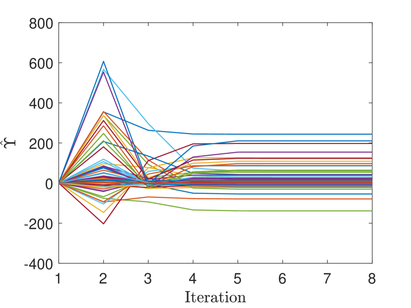
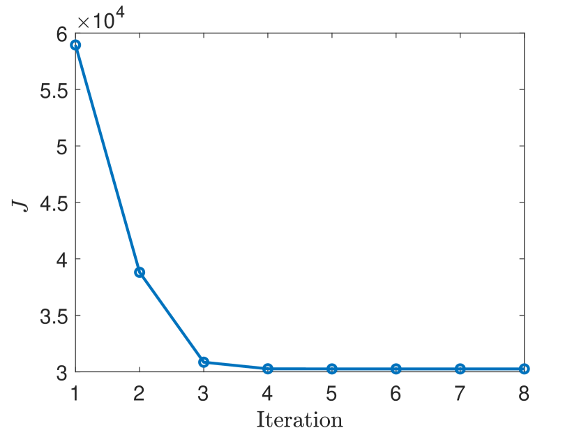
Refer to caption
(a) Evolution of Υ^^Υ\hat{\Upsilon}
Refer to caption
(b) Evolution of J𝐽J.
Figure 1: Evolution of Υ^^Υ\hat{\Upsilon} and the performance index with respect to iterations.
Refer to caption
Figure 2: ADP controller of PI.
Figure 3: Comparison between the initial controller and the ADP controller for regenerative chatter in metal cutting.
TABLE I: Comparison of Alg. 1 and semi-discretization.
Performance index
Algorithm 1 Model-based DLQR Discrete-time ADP
3.02561043.0256superscript1043.0256\cdot 10^{4} 3.26141043.2614superscript1043.2614\cdot 10^{4} 4.82031044.8203superscript1044.8203\cdot 10^{4}
Refer to caption
Figure 4: Evolution of the performance index using noisy data.

V-B CAVs in Mixed Traffic

Refer to caption
Figure 5: A string of HDVs and an AV.

Consider a string of two HDVs and one AV as shown in Fig. 5, where hisubscript𝑖h_{i} denotes the bumper-to-bumper distance between the i𝑖ith vehicle and (i1)𝑖1(i-1)th vehicle, and visubscript𝑣𝑖v_{i} denotes the velocity of the i𝑖ith vehicle. Define Δhi=hihΔsubscript𝑖subscript𝑖superscript\Delta h_{i}=h_{i}-h^{*} and Δvi=vivΔsubscript𝑣𝑖subscript𝑣𝑖superscript𝑣\Delta v_{i}=v_{i}-v^{*}, where (h,v)superscriptsuperscript𝑣(h^{*},v^{*}) is the equilibrium of the vehicles. hsuperscripth^{*} depends on the human parameters and v=v1superscript𝑣subscript𝑣1v^{*}=v_{1}. Assuming the velocity of the leading vehicle is constant, and considering the time-delay effect caused by human drivers’ reaction time, the system can be described as a linear time-delay system (1) with x=[Δh2,Δv2,Δh3,Δv3]𝑥superscriptΔsubscript2Δsubscript𝑣2Δsubscript3Δsubscript𝑣3topx=[\Delta h_{2},\Delta v_{2},\Delta h_{3},\Delta v_{3}]^{\top}, A=[0100000001010000]𝐴matrix0100000001010000A=\begin{bmatrix}0&-1&0&0\\ 0&0&0&0\\ 0&1&0&-1\\ 0&0&0&0\end{bmatrix}, Ad=[0000α2c(α2+β2)0000000000]subscript𝐴𝑑matrix0000subscript𝛼2superscript𝑐subscript𝛼2subscript𝛽20000000000A_{d}=\begin{bmatrix}0&0&0&0\\ \alpha_{2}c^{*}&-(\alpha_{2}+\beta_{2})&0&0\\ 0&0&0&0\\ 0&0&0&0\end{bmatrix}, and B=[0001]𝐵matrix0001B=\begin{bmatrix}0\\ 0\\ 0\\ 1\end{bmatrix}, where α2subscript𝛼2\alpha_{2} and β2subscript𝛽2\beta_{2} denote the human driver parameters and csuperscript𝑐c^{*} is the derivative of the range policy [12, 11]. In the simulation, the human parameters are set as α2=0.1subscript𝛼20.1\alpha_{2}=0.1, β2=0.2subscript𝛽20.2\beta_{2}=0.2, τ=1.2𝜏1.2\tau=1.2, and c=1.5708superscript𝑐1.5708c^{*}=1.5708. The weighting matrix of the performance index is Q=diag([1,1,10,10])𝑄diag111010Q=\text{diag}([1,1,10,10]), and R=1𝑅1R=1. The initial state of the system is [x0(θ)]i=30j=110sinwi,jθ+[χ]isubscriptdelimited-[]subscript𝑥0𝜃𝑖30superscriptsubscript𝑗110subscript𝑤𝑖𝑗𝜃subscriptdelimited-[]𝜒𝑖[x_{0}(\theta)]_{i}=30\sum_{j=1}^{10}\sin{w_{i,j}\theta}+[\chi]_{i} for i=1,2,3,4𝑖1234i=1,2,3,4, where wi,jsubscript𝑤𝑖𝑗w_{i,j} and [χ]isubscriptdelimited-[]𝜒𝑖[\chi]_{i} are randomly sampled from the uniform distribution over [10,10]1010[-10,10] and [30,30]3030[-30,30] respectively. The initial admissible controller is u1(xt)=K0,1x(t)τ0K1,1(θ)xt(θ)dθsubscript𝑢1subscript𝑥𝑡subscript𝐾01𝑥𝑡superscriptsubscript𝜏0subscript𝐾11𝜃subscript𝑥𝑡𝜃differential-d𝜃u_{1}(x_{t})=-K_{0,1}x(t)-\int_{-\tau}^{0}K_{1,1}(\theta)x_{t}(\theta)\mathrm{d}\theta, with K0,1=[0.08970.27720.30.5196]subscript𝐾01matrix0.08970.27720.30.5196K_{0,1}=\begin{bmatrix}-0.0897&-0.2772&-0.3&0.5196\end{bmatrix} and K1,1(θ)=0subscript𝐾11𝜃0K_{1,1}(\theta)=0. The exploration noise is set as ud(t)=i=1200sinωitsubscript𝑢𝑑𝑡superscriptsubscript𝑖1200subscript𝜔𝑖𝑡u_{d}(t)=\sum_{i=1}^{200}\sin{\omega_{i}t}, where ωisubscript𝜔𝑖\omega_{i} is randomly sampled from a independent uniform distribution over [100,100]100100[-100,100]. u=u1+ud𝑢subscript𝑢1subscript𝑢𝑑u=u_{1}+u_{d} is applied to collect the input-state data from the system. The basis functions are same as these in the example of regenerative chatter in metal cutting. The analytical expressions of the optimal values K0subscriptsuperscript𝐾0K^{*}_{0} and K1subscriptsuperscript𝐾1K^{*}_{1} are derived by the method in [11], where the precise model is assumed known.
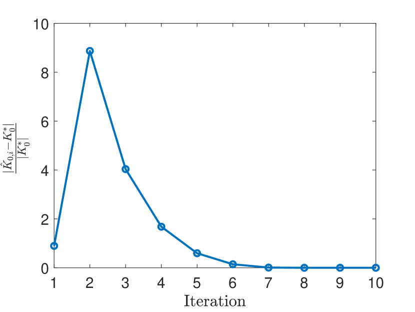
Refer to caption
Refer to caption
Figure 6: Convergence of K^0,isubscript^𝐾0𝑖\hat{K}_{0,i} and K^1,i(θ)subscript^𝐾1𝑖𝜃\hat{K}_{1,i}(\theta) to the optimal values K0subscriptsuperscript𝐾0{K}^{*}_{0} and K1(θ)subscriptsuperscript𝐾1𝜃{K}^{*}_{1}(\theta) by PI algorithm.
Refer to caption
Figure 7: ADP controller of PI
Figure 8: Comparison between the initial controller and the ADP controller for CAVs.

For our proposed data-driven PI algorithm, the aforementioned initial admissible control u1subscript𝑢1u_{1} is applied to start the algorithm. The threshold is δ=103𝛿superscript103\delta=10^{-3}. The convergence of K^0subscript^𝐾0\hat{K}_{0} and K^1,isubscript^𝐾1𝑖\hat{K}_{1,i} are shown in Fig. 6. At the last iteration of PI, |K^0,10K0||K0|=0.0008subscript^𝐾010subscriptsuperscript𝐾0subscriptsuperscript𝐾00.0008\frac{|\hat{K}_{0,10}-K^{*}_{0}|}{|K^{*}_{0}|}=0.0008 and K^1,10K1K1=0.0137subscriptnormsubscript^𝐾110subscriptsuperscript𝐾1subscriptnormsubscriptsuperscript𝐾10.0137\frac{||\hat{K}_{1,10}-K^{*}_{1}||_{\infty}}{||K^{*}_{1}||_{\infty}}=0.0137. Therefore, the proposed data-driven PI algorithm can find a sub-optimal solution. The performance comparisons of the initial controller and the ADP controller are shown in Fig. 8. Because x1subscript𝑥1x_{1} and x2subscript𝑥2x_{2} are the states of the HDV2, which cannot be influenced by the controller for the AV, they are not plotted in the figure. From the figure, it is seen that with the ADP controller, x3subscript𝑥3x_{3} converges to the equilibrium more quickly than the initial controller. For the values of performance index, J(x0,u1)=1.4627105𝐽subscript𝑥0subscript𝑢11.4627superscript105J(x_{0},u_{1})=1.4627\cdot 10^{5} and J(x0,u10)=4.7288104𝐽subscript𝑥0subscript𝑢104.7288superscript104J(x_{0},u_{10})=4.7288\cdot 10^{4}. Therefore, the proposed data-driven PI algorithm can minimize the performance index and improve the performance of the closed-loop system as a consequence.

VI Conclusions

This paper has proposed for the first time a novel data-driven PI algorithm for a class of linear time-delay systems described by DDEs. The first major contribution of this paper is to generalize the well-known Kleinman algorithm [47] – a model-based PI algorithm – from linear time-invariant systems to linear time-delay systems. The second major contribution of this paper is that we have combined the proposed model-based PI algorithm and RL techniques to develop a data-driven PI algorithm for solving the direct adaptive optimal control problem for linear time-delay systems with completely unknown dynamics. The efficacy of the proposed learning-based adaptive optimal control design methods has been validated by means of two real-world applications arising from metal cutting and connected vehicles. Our future work will be directed at extending the proposed learning-based control methodology to other practically important classes of time-delay systems such as nonlinear systems and multi-agent systems.

References

  • [1] V. Kolmanovskii and A. Myshkis, Introduction to the Theory and Applications of Functional Differential Equations. New York, NY: Kluwer Academic Publishers, 1999.
  • [2] J. K. Hale and S. M. V. Lunel, Introduction to functional differential equations. New York, NY: Springer-Verlag, 1993.
  • [3] I. Karafyllis and Z. P. Jiang, Stability and Stabilization of Nonlinear Systems. London, UK: Springer-Verlag, 2011.
  • [4] P. Pepe and Z. P. Jiang, “A Lyapunov–Krasovskii methodology for ISS and iISS of time-delay systems,” Syst Control Lett, vol. 55, no. 12, pp. 1006–1014, 2006.
  • [5] N. Yeganefar, P. Pepe, and M. Dambrine, “Input-to-state stability of time-delay systems: A link with exponential stability,” IEEE Trans. Autom. Control, vol. 53, no. 6, pp. 1526–1531, 2008.
  • [6] L. Xie, E. Fridman, and U. Shaked, “Robust Hsubscript𝐻{H}_{\infty} control of distributed delay systems with application to combustion control,” IEEE Trans. Autom. Control, vol. 46, no. 12, pp. 1930–1935, 2001.
  • [7] S. Xie and L. Xie, “Stabilization of a class of uncertain large-scale stochastic systems with time delays,” Automatica, vol. 36, no. 1, pp. 161–167, 2000.
  • [8] Y. He, Q.-G. Wang, L. Xie, and C. Lin, “Further improvement of free-weighting matrices technique for systems with time-varying delay,” IEEE Trans. Autom. Control, vol. 52, no. 2, pp. 293–299, 2007.
  • [9] H. Gao and T. Chen, “New results on stability of discrete-time systems with time-varying state delay,” IEEE Trans. Autom. Control, vol. 52, no. 2, pp. 328–334, 2007.
  • [10] J. Lam, H. Gao, and C. Wang, “Stability analysis for continuous systems with two additive time-varying delay components,” Syst Control Lett, vol. 56, no. 1, pp. 16–24, 2007.
  • [11] J. I. Ge and G. Orosz, “Optimal control of connected vehicle systems with communication delay and driver reaction time,” IEEE Trans. Intell. Transp. Syst., vol. 18, no. 8, pp. 2056–2070, 2017.
  • [12] M. Huang, Z. P. Jiang, and K. Ozbay, “Learning-based adaptive optimal control for connected vehicles in mixed traffic: robustness to driver reaction time,” IEEE Trans. Cybern., vol. 52, no. 6, pp. 5267–5277, 2022.
  • [13] G. Stépán, “Delay effects in the human sensory system during balancing,” Phil. Trans. R. Soc. A., vol. 367, pp. 1195–212, 04 2009.
  • [14] H. Gao, T. Chen, and J. Lam, “A new delay system approach to network-based control,” Automatica, vol. 44, no. 1, pp. 39–52, 2008.
  • [15] C. V. Hollot, V. Misra, D. Towsley, and W. Gong, “Analysis and design of controllers for AQM routers supporting TCP flows,” IEEE Trans. Autom. Control, vol. 47, no. 6, pp. 945–959, 2002.
  • [16] S. Liu, L. Xie, and H. Zhang, “Distributed consensus for multi-agent systems with delays and noises in transmission channels,” Automatica, vol. 47, no. 5, pp. 920–934, 2011.
  • [17] Y. Tamg, H. Gao, W. Zhang, and J. Jurths, “Leader-following consensus of a class of stochastic delayed multi-agent systems with partial mixed impulses,” Automatica, vol. 53, no. 1, pp. 346–354, 2015.
  • [18] I. T. Vyhlidal, Analysis and Synthesis of Time Delay System Spectrum. PhD thesis, Dept. Mech. Eng., Czech Technical Univ. in Prague, Prague, Czechia, 2003.
  • [19] D. Eller, J. Aggarwal, and H. Banks, “Optimal control of linear time-delay systems,” IEEE Trans. Autom. Control, vol. 14, no. 6, pp. 678–687, 1969.
  • [20] D. Ross and I. Flügge-Lotz, “An optimal control problem for systems with differential-difference equation dynamics,” SIAM J. Control Optim., vol. 7, no. 4, pp. 609–623, 1969.
  • [21] D. Ross, “Controller design for time lag systems via a quadratic criterion,” IEEE Trans. Autom. Control, vol. 16, no. 6, pp. 664–672, 1971.
  • [22] J. S. Gibson, “Linear-quadratic optimal control of hereditary differential systems: Infinite dimensional Riccati equations and numerical approximations,” SIAM J. Control Optim., vol. 21, no. 1, pp. 95–139, 1983.
  • [23] H. T. Banks, I. G. Rosen, and K. Ito, “A spline based technique for computing Riccati operators and feedback controls in regulator problems for delay equations,” SIAM J. Sci. Comput., vol. 5, no. 4, pp. 830–855, 1984.
  • [24] J. A. Burns, E. W. Sachs, and L. Zietsman, “Mesh independence of Kleinman–Newton iterations for Riccati equations in Hilbert space,” SIAM J. Control Optim., vol. 47, no. 5, pp. 2663–2692, 2008.
  • [25] V. Mnih, K. Kavukcuoglu, D. Silver, A. Graves, I. Antonoglou, D. Wierstra, and M. Riedmiller, “Playing Atari with deep reinforcement learning,” arXiv e-prints, p. arXiv:1312.5602, Dec. 2013.
  • [26] D. Silver, A. Huang, C. J. Maddison, A. Guez, L. Sifre, G. van den Driessche, J. Schrittwieser, I. Antonoglou, V. Panneershelvam, M. Lanctot, S. Dieleman, D. Grewe, J. Nham, N. Kalchbrenner, I. Sutskever, T. Lillicrap, M. Leach, K. Kavukcuoglu, T. Graepel, and D. Hassabis, “Mastering the game of Go with deep neural networks and tree search,” Nature, vol. 529, pp. 484–489, Jan. 2016.
  • [27] Y. Jiang and Z. P. Jiang, Robust Adaptive Dynamic Programming. NJ, USA: Wiley-IEEE Press, 2017.
  • [28] F. L. Lewis and D. Liu, Reinforcement Learning and Approximate Dynamic Programming for Feedback Control. NJ, USA: Wiley-IEEE Press, 2013.
  • [29] L. Cui, K. Ozbay, and Z. P. Jiang, “Combined longitudinal and lateral control of autonomous vehicles based on reinforcement learning,” in 2021 American Control Conference (ACC), pp. 1929–1934, 2021.
  • [30] L. Cui, S. Wang, J. Zhang, D. Zhang, J. Lai, Y. Zheng, Z. Zhang, and Z. P. Jiang, “Learning-based balance control of wheel-legged robots,” IEEE Robotics and Automation Letters, vol. 6, no. 4, pp. 7667–7674, 2021.
  • [31] Z. P. Jiang, T. Bian, and W. Gao, “Learning-based control: A tutorial and some recent results,” Found. Trends Syst. Control, vol. 8, no. 3, pp. 176–284, 2020.
  • [32] Y. Jiang and Z. P. Jiang, “Computational adaptive optimal control for continuous-time linear systems with completely unknown dynamics,” Automatica, vol. 48, no. 10, pp. 2699–2704, 2012.
  • [33] T. Bian and Z. P. Jiang, “Value iteration and adaptive dynamic programming for data-driven adaptive optimal control design,” Automatica, vol. 71, pp. 348–360, 2016.
  • [34] T. Bian and Z. P. Jiang, “Reinforcement learning and adaptive optimal control for continuous-time nonlinear systems: a value iteration approach,” IEEE Trans. Neural Netw. Learn. Syst., in press, 2021.
  • [35] W. Gao and Z. Jiang, “Adaptive dynamic programming and adaptive optimal output regulation of linear systems,” IEEE Trans. Autom. Control, vol. 61, no. 12, pp. 4164–4169, 2016.
  • [36] B. Pang and Z. P. Jiang, “Adaptive optimal control of linear periodic systems: an off-policy value iteration approach,” IEEE Trans. Autom. Control, vol. 66, no. 2, pp. 888–894, 2021.
  • [37] M. Huang, Z. P. Jiang, M. Malisoff, and L. Cui, “Robust autonomous driving with human in the loop,” in Handbook of Reinforcement Learning and Control (K. G. Vamvoudakis, Y. Wan, F. L. Lewis, and D. Cansever, eds.), pp. 62–77, New York, NY, USA: Springer, 2021.
  • [38] S. A. Asad Rizvi, Y. Wei, and Z. Lin, “Model-free optimal stabilization of unknown time delay systems using adaptive dynamic programming,” in Proc. IEEE Conf. Decis. Control., pp. 6536–6541, 2019.
  • [39] Q.-L. Wei, H.-G. Zhang, D.-R. Liu, and Y. Zhao, “An optimal control scheme for a class of discrete-time nonlinear systems with time delays using adaptive dynamic programming,” Acta Automatica Sinica, vol. 36, no. 1, pp. 121–129, 2010.
  • [40] Y. Liu, H. Zhang, Y. Luo, and J. Han, “ADP based optimal tracking control for a class of linear discrete-time system with multiple delays,” Journal of the Franklin Institute, vol. 353, no. 9, pp. 2117–2136, 2016.
  • [41] H. Zhang, C. Qin, B. Jiang, and Y. Luo, “Online adaptive policy learning algorithm for Hsubscript𝐻H_{\infty} state feedback control of unknown affine nonlinear discrete-time systems,” IEEE Trans. Cybern., vol. 44, no. 12, pp. 2706–2718, 2014.
  • [42] H. Zhang, R. Song, Q. Wei, and T. Zhang, “Optimal tracking control for a class of nonlinear discrete-time systems with time delays based on heuristic dynamic programming,” IEEE Trans. Neural Netw., vol. 22, no. 12, pp. 1851–1862, 2011.
  • [43] B. Wang, D. Zhao, C. Alippi, and D. Liu, “Dual heuristic dynamic programming for nonlinear discrete-time uncertain systems with state delay,” Neurocomputing, vol. 134, pp. 222–229, 2014.
  • [44] J. G. Rueda-Escobedo, E. Fridman, and J. Schiffer, “Data-driven control for linear discrete-time delay systems,” IEEE Trans. Autom. Control, pp. 1–1, 2021.
  • [45] R. Moghadam, S. Jagannathan, V. Narayanan, and K. Raghavan, Optimal Adaptive Control of Partially Uncertain Linear Continuous-Time Systems with State Delay, pp. 243–272. Cham: Springer International Publishing, 2021.
  • [46] R. Moghadam and S. Jagannathan, “Optimal adaptive control of uncertain nonlinear continuous-time systems with input and state delays,” IEEE Trans. Neural Netw. Learn. Syst., pp. 1–10, 2021.
  • [47] D. Kleinman, “On an iterative technique for Riccati equation computations,” IEEE Trans. Autom. Control, vol. 13, no. 1, pp. 114–115, 1968.
  • [48] R. F. Curtain, An Introduction to Infinite-Dimensional Linear Systems Theory. New York, NY: Springer, 1995.
  • [49] Y. Eidelman, V. Milman, and A. Tsolomitis, Functional Analysis, An Introduction. Rhode Island, USA: American Mathematical Society, 2004.
  • [50] K. Gu, V. L. Kharitonov, and J. Chen, Stability of Time-Delay Systems. Boston, MA: Birkhäuser, 2003.
  • [51] E. Fridman, Introduction to Time-Delay Systems Analysis and Control. Switzerland: Springer, 2014.
  • [52] R. E. Kalman, “Contributions to the theory of optimal control,” Boletin Sociedad Matematica Mexicana, vol. 5, no. 2, pp. 102–119, 1960.
  • [53] K. Uchida and E. Shimemura, “Closed-loop properties of the infinite-time linear-quadratic optimal regulator for systems with delays,” Int. J. Control, vol. 43, no. 3, pp. 773–779, 1986.
  • [54] C. C. Pugh, Real Mathematical Analysis, 2nd Edition. AG Switzerland: Springer International Publishing, 2015.
  • [55] M. J. D. Powell, Approximation Theory and Methods. New York, NY: Cambridge University Press, 1981.
  • [56] Z. P. Jiang, C. Prieur, and A. Astolfi (Editors), Trends in Nonlinear and Adaptive Control: A Tribute to Laurent Praly for His 65th Birthday,. NY, USA: Springer Nature, 2021.
  • [57] K. J. Åström and B. Wittenmark, Adaptive control, 2nd Edition. MA, USA: Addison-Wesley, 1997.
  • [58] C. Mei, J. G. Cherng, and Y. Wang, “Active control of regenerative chatter during metal cutting process,” J. Manuf. Sci. Eng., vol. 128, pp. 346–349, 06 2005.
  • [59] T. Insperger and G. Stépán, “Semi-discretization method for delayed systems,” Int. J. Numer. Methods Eng., vol. 55, no. 5, pp. 503–518, 2002.