$py$GWBSE: A high throughput workflow package for GW-BSE calculations

Abstract

We develop an open-source python workflow package, pyGWBSE to perform automated first-principles calculations within the GW-BSE (Bethe-Salpeter) framework. GW-BSE is a many body perturbation theory based approach to explore the quasiparticle (QP) and excitonic properties of materials. The GW approximation has proven to be effective in accurately predicting bandgaps of a wide range of materials by overcoming the bandgap underestimation issues of the more widely used density functional theory (DFT). The BSE formalism, in spite of being computationally expensive, produces absorption spectra directly comparable with experimental observations. The pyGWBSE package achieves complete automation of the entire multi-step GW-BSE computation, including the convergence tests of several parameters that are crucial for the accuracy of these calculations. pyGWBSE is integrated with Wannier90, a program for calculating maximally-localized wannier functions, allowing the generation of QP bandstructures. pyGWBSE also enables the automated creation of databases of metadata and data, including QP and excitonic properties, which can be extremely useful for future material discovery studies in the field of ultra-wide bandgap semiconductors, electronics, photovoltaics, and photocatalysis.

1 Introduction

Obtaining materials with properties that are optimized for a particular application traditionally relies on time-consuming and expensive experimental work. However, in recent years an alternative paradigm in the field of material discovery has emerged through the availability of modern massive supercomputing resources, development of first-principles methodologies, and ingenious computational algorithms. These advancements have pushed the boundaries of materials simulations, making them faster, more cost-effective, efficient and accurate. Consequently, high-throughput materials simulations have emerged as a tool for creating large databases and screening materials from these databases to identify candidate materials for applications in photocatalysis singh2019robust ; wu2013first , energy storage kirklin2013high ; hautier2011phosphates , piezoelectrics choudhary2020high , electrocatalysis greeley2006computational etc.

However, applying similar approaches to applications related to optical and transport properties of materials have been hindered by a few technical obstacles. Density functional theory (DFT), the most widely used tool in computational high-throughput materials discovery studies are designed to explore ground state properties of a system and has been remarkably successful in predicting structural, mechanical, electronic, and thermal properties jones2015density . However, studying the excited state properties of a system, such as optoelectronic or transport properties using DFT requires the interpretation of Kohn-Sham (KS) eigenvalues as energies involved in adding an electron to a many-electron system or subtracting one from it (QP energies). Following such a procedure, one often encounters the infamous bandgap underestimation problem due to the derivative discontinuity of the exchange-correlation energy perdew1985density .

A more rigorous approach to computing QP energies and accurate bandgap is applying many body perturbation theory (MBPT) within the GW approximation hedin1965new . Using this formalism, one computes the QP energies by calculating the first-order perturbative correction to the KS eigenvalues by approximating self-energy as a product of one particle Green’s function (G) and screened Coulomb interaction (W). It has been shown that MBPT within the GW approximation is particularly useful in computing QP properties of a wide variety of semiconductors and insulators onida2002electronic without requiring any ad-hoc introduction of mixing parameters like those needed for hybrid functionals used in DFT muscat2001prediction ; vines2017systematic .

Additionally, the study of QP properties using GW formalism enables us to compute several transport properties of materials that are inaccessible from a DFT calculation. For example, QP lifetimes calculated from GW calculations can be directly used to estimate impact ionization rates, a very useful parameter in the study of high-field transport of wide bandgap materials kotani2010impact . In case of low field transport, in addition to the obvious importance darancet2007ab of including GW corrections to KS eigenvalues and carrier mobilities, it has been shown that one needs to include the effects of GW correction on the orbital character of the relevant KS wavefunctions to obtain accurate transport properties of molecular junctions rangel2011transport .

The optical and transport properties of semiconductors to a large extent are defined by the presence of intentional dopants or unintentional defects. GW formalism has emerged as a powerful approach that complements experiments and has become reliable enough to serve as a predictive tool for crucial point defect properties such as charge transition levels and F-center photoluminescence spectra in semiconductors biswas2019electronic ; freysoldt2014first . Moreover, calculations based on MBPT using GW approximation has been successfully applied to estimate non-radiative recombinations such as Auger recombination rates kioupakis2011indirect ; mcallister2015auger which are very useful for optical applications. Auger recombination mechanism has been shown to cause significant efficiency loss in InGaN-based light-emitting diodes (LEDs), when operating at high injected carrier densities.

The necessity of the BSE methodology lies in the fact that even after including GW corrections the optical spectrum calculated within the independent-particle picture shows significant deviations from experimental results, as not only the absorption energies can be wrong, but often the oscillator strength of the peaks can deviate from the experiment by a factor of 2 or more. Moreover, it can not describe bound exciton states, which are particularly important in systems of reduced dimensions ugeda2014giant . The reason being, independent particle picture can’t include electron-hole interactions (excitonic effects) which requires an effective two-body approach rohlfing2000electron . This can be achieved by evaluating the two-body Green’s function G₂ and formulating an equation of motion for G₂, known as the Bethe-Salpeter equation (BSE) rohlfing2000electron .

Despite its obvious indispensability, high-throughput computational material discovery studies for light-matter interaction related applications so far have not been able to incorporate the QP or excitonic properties of materials using GW-BSE formalism. Two main challenges for such an endeavor is the efficient convergence of multiple parameters and the tractability of the huge computational cost associated with the multi-step GW-BSE formalism. GW-BSE calculations are extremely sensitive to multiple interdependent convergence parameters such as the number of bands included in the GW self-energy calculation or the number of $k$-points used to sample the Brillouin zone (BZ) in the BSE calculation etc.

In this article, we introduce the open-source Python package, $py$GWBSE, which automates the entire GW-BSE calculation using first-principles simulations software Vienna Ab-initio Software Package ($VASP$) hafner2008ab . This package enables automated input file generation, submission to supercomputing platforms, analysis of post-simulation data, and storage of metadata and data in a MongoDB database. Moreover, pyGWBSE is capable of handling multiple convergence parameters associated with the GW-BSE formalism. Using this package, high-throughput computation of various electronic and optical properties is possible in a systematic and efficient manner. For example, the QP energies, bandstructures, and density of states can be computed using both the one-shot G₀W₀ and partially self-consistent GW₀ level of the GW formalism. The package enables automated BSE computations yielding the real and imaginary part of the dielectric function (incorporating electron-hole interaction), the exciton energies, and their corresponding oscillator strengths. DFT bandstructures, orbital resolved density of states (DOS), electron/hole effective masses, band-edges, real and imaginary parts (absorption spectra) of the dielectric function, and static dielectric tensors can also be computed using $py$GWBSE.

The package is being continuously developed and the latest version can be obtained from the GitHub repository at ${\it https://github.com/cmdlab/pyGWBSE}$. $py$GWBSE is built upon existing open source Python packages such as, $pymatgen$ ong2013python , $Fireworks$ jain2015Fireworks , and $\it atomate$ mathew2017atomate . To obtain the QP bandstructure we use the $Wannier90$ mostofi2008wannier90 , a program for calculating maximally-localized Wannier functions to perform the interpolation required to obtain QP bandstructure with reduced computational cost.

$py$GWBSE enables high-throughput simulations of highly reliable and efficient $ab$-$initio$ approaches thus enabling future materials screening studies, the creation of large databases of high-quality computed properties of materials, and in turn machine learning model development. Hence, $py$GWBSE could serve as a catapult to the next generation of technological advances in the field of power electronics, optoelectronics, photovoltaics, photocatalysis, etc.

In the following sections, we present an overview of the underlying methodology, describe the workflow architecture, discuss the algorithms that were developed to perform the multi-step convergences, and benchmark the results obtained from the $py$GWBSE workflow against experimental data in the literature.

2 $py$GWBSE: Underlying Methodology and Codes

The first principles calculations in the $py$GWBSE package are performed using one of the most well-known packages, $VASP$. $VASP$ is a first principles computer program for atomic scale materials modeling. It is capable of using the projector-augmented wave (PAW) method blochl1994projector and it comes with a rigorously tested pseudopotential library. $VASP$ provides the accuracy of the full-potential linearized augmented-plane-wave (FLAPW) singh1994planes method, but is computationally less expensive than most of the traditional plane wave-based methods hafner2008ab . Currently, in addition to DFT, GW, and BSE, it supports various other post-DFT methods such as TD-DFT, ACFDT, 2nd-order Møller-Plesset perturbation theory and is under constant development, which opens up the possibility of implementing these methodologies in the $py$GWBSE workflow in the future. Additionally, $VASP$ is very efficiently parallelized and can utilize the potential of modern computers of both CPU and GPU-based architectures.

The $py$GWBSE package is capable of computing several material properties using the DFT, GW, and BSE methodologies. A brief summary of GW-BSE methodology has been presented in section 2.1.1 (GW) and 2.1.2 (BSE). Using $py$GWBSE, properties such as bandstructures, the orbital resolved density of states (DOS), electron/hole effective masses, band-edges, real and imaginary part (absorption spectra) of the dielectric function ($\epsilon(\omega)$), and static dielectric tensors can be computed using the DFT methodology. In the $py$GWBSE package, the GW formalism can be used to compute QP energies both at one-shot G₀W₀ and partially self-consistent GW₀ level of accuracy. The package uses maximally localized wannier functions (MLWF) to compute the electronic structure at the QP level of accuracy but at a significantly reduced computation cost. Using this package, the BSE methodology can be used to compute the real and imaginary parts of the dielectric function (incorporating electron-hole interaction), the exciton energies, and their corresponding oscillator strengths.

2.1 Theoretical background and parameter convergence in $py$GWBSE

In the following two sections, we describe the $py$GWBSE package’s computational framework with a particular emphasis on all the crucial computational parameters which are needed to be converged for obtaining accurate results. Fig. 1 provides a condensed diagrammatic representation of the GW-BSE framework described in the following two subsections; showing the interconnection between the key equations and the various physical quantities. Detailed discussions about the GW-BSE methodology can be found in several review articles onida2002electronic ; leng2016gw ; faber2014excited ; blase2018bethe .

Additionally, we also present the rationale behind the strategies that we adopt to reduce the computational cost of the convergence calculations and thus make the computations more time-efficient. A discussion of the convergence parameters for the DFT ground state calculations can be found in the existing literature jain2011high ; kresse2018j . In these studies, plane wave energy cutoff was set to 1.3 times the maximum energy cutoff specified in the pseudopotentials and $k$-grid set as (500)/n points, where n represents the number of atoms in the unit cell distributed as uniformly as possible in $k$-space. It resulted in total energy convergence of 15 meV/atom for 96$\%$ of 182 chemically diverse materials jain2011high . In the following, sections 2.1.1 and 2.1.2, we discuss that the same choice for the plane wave energy cutoff but a higher $k$-grid density is required to converge the GW-BSE calculations. Additionally, other convergence parameters are needed for the GW-BSE calculations, and the strategies to converge them are elaborated through examples.

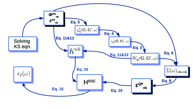
Figure 1: A schematic summarizing the GW-BSE framework. All the equations as well as the key quantities mentioned in section 2.1.1 and section 2.1.2 are drawn to provide a condensed visual representation.

2.1.1 Obtaining converged QP energies using GW methodology

The QP energies are the energies for adding an electron to a many-electron system or subtracting one from it. Within the MBPT they can be calculated by solving the following equation hedin1965new ,

$$(T+V_{n-e}+V_{H}-E_{n{\bf k}}^{QP})\psi^{QP}_{n{\bf k}}({\bf r})+\int d^{3}{\bf r^{\prime}}\Sigma({\bf r},{\bf r^{\prime}},E_{n{\bf k}}^{QP})\psi^{QP}_{n{\bf k}}({\bf r^{\prime}})=0$$ (1)

where, $T$ is the kinetic energy operator, $V_{n-e}$ is the operator to account for the nuclear(ion)-electronic interaction, $V_{H}$ is the Hartree potential, $\Sigma$ is the self-energy operator and $\bf r$ is the position vector of the electron. $E_{n{\bf k}}^{QP}$ and $\psi^{QP}_{n{\bf k}}$s are the QP energies and wavefunctions for $n^{th}$ band with wavevector $\bf k$.

GW approximation provides a practical route to compute the self energy operator, $\Sigma({\bf r},{\bf r^{\prime}},\omega)$, from KS wavefunctions, $\psi_{n{\bf k}}$, and energies, $\epsilon_{n{\bf k}}$, through one particle Green’s function, $G({\bf r},{\bf r^{\prime}},\omega)$.hedin1965new ; hybertsen1986electron ; shishkin2006implementation Within the GW approximation $\Sigma$ can be written as,

$$\Sigma({\bf r},{\bf r^{\prime}},\omega)=\frac{i}{4\pi}\int_{-\infty}^{\infty}e^{i\omega^{\prime}\delta}G({\bf r},{\bf r^{\prime}},\omega+\omega^{\prime})W({\bf r},{\bf r^{\prime}},\omega^{\prime})d\omega^{\prime}$$ (2)

where, $W$ is the screened Coulomb interaction, $\omega$ is the frequency and $\delta$ is the positive infinitesimal.

$W$ can be computed from $\psi_{n{\bf k}}$ and $\epsilon_{n{\bf k}}$ through independent particle polarizability and frequency dependent dielectric matrix utilizing the following three equations and taking advantage of the Random Phase Approximation (RPA) hybertsen1987ab .

$$W_{\bf q}({\bf G},{\bf G^{\prime}},\omega)=4\pi e^{2}\frac{1}{\lvert{\bf q}+{\bf G}\rvert}\epsilon^{-1}_{\bf q}({\bf G},{\bf G^{\prime}},\omega)\frac{1}{\lvert{\bf q}+{\bf G^{\prime}}\rvert}$$ (3)

The dielectric matrix, $\epsilon_{\bf q}({\bf G},{\bf G^{\prime}},\omega)$ is related to $\chi$ as hybertsen1987ab ,

$$\epsilon_{\bf q}({\bf G},{\bf G^{\prime}},\omega)=\delta_{{\bf G}{\bf G^{\prime}}}-\frac{4\pi e^{2}}{\lvert{\bf q}+{\bf G}\rvert\lvert{\bf q}+{\bf G^{\prime}}\rvert}\chi^{0}_{\bf q}({\bf G},{\bf G^{\prime}},\omega)$$ (4)

Within RPA, independent particle polarizibility, $\chi^{0}_{\bf q}({\bf G},{\bf G^{\prime}},\omega)$, is calculated as hybertsen1987ab ,

$$\chi^{0}_{\bf q}({\bf G},{\bf G^{\prime}},\omega)=\Omega^{-1}\Sigma_{n,n^{\prime},{\bf k}}2w_{\bf k}(f_{n,{{\bf k}-{\bf q}}}-f_{n,{\bf k}})\times\\ \frac{\langle\psi_{n^{\prime}{\bf k}-{\bf q}}\lvert e^{-i({\bf q}+{\bf G}){\bf r}}\rvert\psi_{n{\bf k}}\rangle\langle\psi_{n{\bf k}}\lvert e^{i({\bf q}+{\bf G^{\prime}}){\bf r^{\prime}}}\lvert\psi_{n^{\prime}{\bf k}-{\bf q}}\rangle}{\omega+\epsilon_{n^{\prime}{\bf k}-{\bf q}}-\epsilon_{n{\bf k}}+i\eta sgn[\epsilon_{n^{\prime}{\bf k}}-\epsilon_{n{\bf k}}]}$$ (5)

where, $w_{\bf k}$ is the $k$-point weight, the $f_{n,{\bf k}}$ are the one electron occupancy of the corresponding states, ${\bf q}$ is the Bloch wave vector, $\bf G$ is the reciprocal lattice vector and $\eta$ is the infinitesimal complex shift.

Once the screened Coulomb interaction, $W$, is computed, the diagonal matrix elements of self-energy operator, $\Sigma(\omega)_{n{\bf k},n{\bf k}}$, can be obtained using hybertsen1986electron ,

$$\Sigma(\omega)_{n{\bf k},n{\bf k}}=\Omega^{-1}\Sigma_{{\bf q}{\bf G}{\bf G^{\prime}}}\Sigma_{n^{\prime}}\frac{i}{2\pi}\int^{\infty}_{0}d{\omega^{\prime}}W_{\bf q}({\bf G},{\bf G^{\prime}},\omega^{\prime})\\ \times\langle\psi_{n{\bf k}}\lvert e^{i({\bf q}+{\bf G}){\bf r}}\rvert\psi_{n^{\prime}{\bf k}-{\bf q}}\rangle\langle\psi_{n^{\prime}{\bf k}-{\bf q}}\lvert e^{-i({\bf q}+{\bf G^{\prime}}){\bf r^{\prime}}}\rvert\psi_{n{\bf k}}\rangle\\ \times(\frac{1}{\omega+\omega^{\prime}-\epsilon_{n^{\prime}{\bf k}-{\bf q}}+i\eta sgn(\epsilon_{n^{\prime}{\bf k}-{\bf q}}-\mu)}+\frac{1}{\omega-\omega^{\prime}-\epsilon_{n^{\prime}{\bf k}-{\bf q}}+i\eta sgn(\epsilon_{n^{\prime}{\bf k}-{\bf q}}-\mu)})$$ (6)

where, $\mu$ is the Fermi energy. In the non-self-consistent GW calculation (also known as G₀W₀) G₀ and W₀ are calculated using KS eigenvalues and eigenfunctions. The wavefunction of QP Hamiltonian (Eqn. 1) is approximated as the DFT wavefunction and the QP energies are computed to first order as,

$$E^{QP}_{n{\bf k}}=Re[\langle\psi_{n{\bf k}}\lvert T+V_{n-e}+V_{H}+\Sigma(E^{QP}_{n{\bf k}})\rvert\psi_{n{\bf k}}\rangle]$$ (7)

Since Eqn. 7 requires the values of $E^{QP}_{n{\bf k}}$, the equation must be solved by iteration. Using the usual Newton-Raphson method for root finding, one can obtain the following update equation hybertsen1986electron ,

$$E^{QP}_{n{\bf k}}\leftarrow E^{QP}_{n{\bf k}}+Z_{n{\bf k}}Re[\langle\psi_{n{\bf k}}\lvert T+V_{n-e}+V_{H}+\Sigma(E^{QP}_{n{\bf k}})\rvert\psi_{n{\bf k}}\rangle-E^{QP}_{n{\bf k}}]$$ (8)

where $Z_{n{\bf k}}$ is the renormalization factor and can be calculated as,

$$Z_{n{\bf k}}=(1-Re(\langle\psi_{n{\bf k}}\lvert\frac{\partial\Sigma(\omega)}{\partial\omega}\rvert\psi_{n{\bf k}}\rangle))^{-1}$$ (9)

The iteration starts from DFT eigenvalues and if one stops after the first iteration the QP energies are obtained within G₀W₀ approximation. One can also continue to obtain QP energies which are self-consistently converged. This scenario is referred to as self-consistent GW approximation (scGW) shishkin2007self .

In the $py$GWBSE workflow, both the G₀W₀ and scGW are implemented. In the partially self-consistent scGW approximation the $G$ is updated self-consistently until convergence is reached but the $W$ is kept unchanged, thus the scGW is also referred to as GW₀. A full update of the $G$ and $W$ is seldom adopted and thus is not included in the $py$GWBSE package. In fact, it has been shown by several studies delaney2004comment ; schone1998self ; tiago2004effect pertaining to free-electron gas, metals, and semiconductors that fully self-consistent GW calculations, without vertex corrections, lead to an overestimation of bandgaps.

There are three crucial parameters in a GW calculation that need to be converged to obtain accurate results, namely-

• Number of plane waves used to expand the screened Coulomb operator, $W_{q}({\bf G},{\bf G^{\prime}},\omega)$. This parameter can be specified by using ENCUTGW in the $VASP$ implementation.

• Number of frequency grid points used in Eqn. 6 for the frequency integration. This parameter can be specified by using NOMEGA in the $VASP$ implementation.

• Number of bands used in Eqn. 5 and 6 for the summation. This parameter can be specified by using NBANDS in the $VASP$ implementation.

Table 1: QP gaps of 9 materials computed using a screened coulomb cutoff, $ENCUTGW$, of 100 eV (E${}^{100}_{g}$), 150 eV (E${}^{150}_{g}$) and 200 eV (E${}^{200}_{g}$). The table shows that 200 eV cutoff is sufficient to converge QP gaps within 0.1 eV for all these materials.

mp-id	Formula	E${}^{100}_{g}$	E${}^{150}_{g}$	E${}^{200}_{g}$
mp-149	Si	1.18	1.20	1.20
mp-390	TiO2	3.89	3.89	3.89
mp-66	C	5.24	5.40	5.46
mp-2133	ZnO	2.66	2.68	2.67
mp-804	GaN	2.84	2.87	2.86
mp-2624	AlSb	1.69	1.69	1.70
mp-1434	MoS2	2.33	2.34	2.34
mp-984	BN	5.45	5.46	5.46
mp-22862	NaCl	7.71	7.72	7.73

Table 2: QP gap of 9 materials computed using NOMEGA of 50 (E${}^{50}_{g}$), 65 (E${}^{65}_{g}$) and 80 (E${}^{80}_{g}$). NOMEGA refers to the number of frequency grid points used in the numerical integration for evaluating the GW self-energy. The table shows that 80 frequency grid points are sufficient to converge QP gaps within 0.1 eV for all of these materials.

mp-id	Formula	E${}^{50}_{g}$	E${}^{65}_{g}$	E${}^{80}_{g}$
mp-149	Si	1.18	1.18	1.18
mp-390	TiO2	3.89	3.80	3.75
mp-66	C	5.24	5.24	5.23
mp-2133	ZnO	2.66	2.48	2.38
mp-804	GaN	2.84	2.84	2.84
mp-2624	AlSb	1.69	1.67	1.66
mp-1434	MoS2	2.33	2.28	2.25
mp-984	BN	5.45	5.44	5.43
mp-22862	NaCl	7.71	7.68	7.67

In principle, the QP energies are to be converged w.r.t all three of the parameters mentioned above. Therefore, in our workflow, we have implemented the convergence tests for QP energies w.r.t. these parameters namely, ENCUTGW, NOMEGA, and NBANDS.

Table 1 and 2 show the QP gaps of 9 materials computed with different values of ENCUTGW and NOMEGA. Table 1 shows the QP gaps computed with ENCUTGW values of 100, 150 and 200 eV, whereas Table 2 shows the QP gaps computed with NOMGEA values of 50, 65, and 80. From Table 1 we can see that, a ENCUTGW value of 150 eV is sufficient for obtaining a QP gap value that is converged within $\sim$ 0.1 eV for almost all the materials except diamond (C), for which we need an ENCUTGW value of 200 eV. Table 2 shows that we need a NOMEGA of 80 to converge the QP gap within 0.1 eV for all the selected materials. Thus, as recommended by the $VASP$ manual, $ENCUTGW$ value of 2/3 $\times$ $ENCUT$ and $NOMEGA$ value of 50–100, would be sufficient to obtain accurate QP energies for a wide range of materials. Furthermore, based on the convergence of the 9 materials in Tables 1 and 2 we surmise that given the variety in the chemical compositions and crystal structures of these materials, it is likely that a value of 200 eV for ENCUTGW and 80 for NOMEGA may be sufficient to converge QP gaps of a variety of other materials within 0.1 eV.

The third parameter, ${\it NBANDS}$, however, needs to be converged for every material. Despite many efforts to eliminate or reduce the need of including large number of empty orbitals in the GW calculation, it still is one of the major computation costs of a GW calculation. While several methods have been proposed to reduce the total number of empty orbitals in a GW calculation such as replacing actual KS orbitals with approximate orbitals generated using a reduced basis set, truncation of the sum over empty orbitals to a reduced number, and adding the contribution of the remaining orbitals within the static (COHSEX) approximation and modified static remainder approach deslippe2013coulomb . These methods are not currently implemented in the $VASP$ package. However, in the future, if these methods are implemented, they can be easily incorporated into the $py$GWBSE package and would reduce the computational costs of GW-BSE calculations significantly. Meanwhile, we strongly suggest performing convergence tests w.r.t NBANDS using $py$GWBSE to obtain accurate results.

2.1.2 Obtaining converged absorption spectra by solving BSE

Studying optical electron-hole excitations is an effective two-body problem. In most cases single-particle picture of individual quasi-electron and quasi-hole excitations are not enough. We need to include electron-hole interactions as well. We can work with two-body Green’s function $G_{2}$ on the basis of the one-body Green’s function $G_{1}$, which can be described by the GW approximation. We can use QP electron and hole states of $G_{1}$ and their QP energies to estimate the electron-hole interactions. The equation of motion for $G_{2}$ is known as the Bethe-Salpeter equation strinati1988application and is very useful in the study of correlated electron-hole excitation states also known as excitons.

Following Strinati strinati1988application , Rohlfing and Louie rohlfing2000electron , the BSE can be written as a generalized eigenvalue problem and the electron-hole excitation states can be calculated through the solution of BSE. For each exciton state $S$, within Tamm-Dancoff approximation the BSE can be written as,

$$(\epsilon^{QP}_{c}-\epsilon^{QP}_{v})A_{vc{\bf k}}+\Sigma_{v^{\prime}c^{\prime}{\bf k^{\prime}}}\langle{{vc{\bf k}}}\lvert K^{eh}\rvert{v^{\prime}c^{\prime}{\bf k^{\prime}}}\rangle=\Omega^{S}A_{vc{\bf k}}$$ (10)

where, $A_{vc{\bf k}}$ is the exciton wavefunction, $\Omega^{S}$ is the excitation energy, $\epsilon^{QP}_{c{\bf k}}$ and $\epsilon^{QP}_{v{\bf k}}$ are the QP energies of the conduction ($\lvert c{\bf k}\rangle$) and valence states ($\lvert v{\bf k}\rangle$) which is computed using the GW methodology discussed in the previous section. The electron-hole interaction kernel, $K^{eh}$, can be separated in two terms, $K^{eh}$ = $K^{d}$ + $K^{x}$, where $K^{d}$ is the screened direct interaction term and $K^{x}$ is the bare exchange interaction term. Within the GW approximation for $\Sigma$, in the basis of the single-particle orbitals in real space ($\phi_{c/v}(\bf x)$, the KS orbitals obtained from DFT calculations), they are defined in the following way,

$$\langle vc\lvert K^{x}\rvert v^{\prime}c^{\prime}\rangle=\int d{\bf x}d{\bf x^{\prime}}\phi^{*}_{c}({\bf x})\phi_{v}({\bf x})v({\bf r},{\bf r^{\prime}})\phi^{*}_{v^{\prime}}({\bf x^{\prime}})\phi_{c^{\prime}}({\bf x^{\prime}})$$ (11)

$$\langle vc\lvert K^{d}\rvert v^{\prime}c^{\prime}\rangle=-\int d{\bf x}d{\bf x^{\prime}}\phi^{*}_{c}({\bf x})\phi_{c^{\prime}}({\bf x})W({\bf r},{\bf r^{\prime}}\mathchar 24635\relax\;\omega=0)\phi^{*}_{v^{\prime}}({\bf x^{\prime}})\phi_{v}({\bf x^{\prime}})$$ (12)

Once we have the solutions of the BSE Hamiltonian, we can construct $\epsilon_{2}(\omega)$ which incorporates excitonic effects from the solutions of the modified BSE,

$$\epsilon_{2}(\omega)=\frac{8\pi^{2}e^{2}}{\omega^{2}}\sum_{s}\lvert\hat{\lambda}\cdot\langle 0\lvert{\bf v}\rvert S\rangle\rvert^{2}\delta(\omega-\Omega^{S})\\ =\frac{8\pi^{2}e^{2}}{\omega^{2}}\sum_{s}\lvert\sum_{vc{\bf k}}A^{S}_{vc{\bf k}}\hat{\lambda}\cdot\langle v{\bf k}\lvert{\bf v}\lvert c{\bf k}\rangle\rvert^{2}\delta(\omega-\Omega^{S})$$ (13)

where $\hat{\lambda}$ is the polarization vector, and ${\bf v}$ is the velocity operator along the direction of the polarization of light, $\hat{\lambda}$. The real part of the dielectric function $\epsilon_{1}(\omega)$, can be obtained by integration of $\epsilon_{2}(\omega)$ over all frequencies via Kramers–Kronig relations.

Converging the BSE absorption spectra with the number of $k$-points used to sample the BZ is one of the most computationally demanding tasks in a GW-BSE calculation. In this study, we propose a strategy to achieve this convergence with a significant reduction in the computational cost involved. We propose to obtain a convergent $\epsilon_{2}(\omega)$ within an independent particle picture (RPA) and use the same $k$-mesh to perform the BSE calculation. This strategy is expected to be useful because of the following reasons.

There are two aspects of the convergence of $\epsilon_{2}(\omega)$ w.r.t $\rho_{k}$. Firstly, due to band dispersion, one needs to include all the occupied-unoccupied transitions throughout the BZ to obtain absorption spectra that are converged. As a result, one needs to use a very dense $k$-grid for materials that have a stronger dispersion of bands near the gap. Secondly, the electron-hole interaction kernel is also dependent on the $k$-grid density, as the integrations described in Eqn. 11 and 12 are evaluated by a plane-wave summation in reciprocal space with the help of Fourier transform. Typically, the band dispersion doesn’t change significantly from DFT to GW bandstructure. Thus one should be able to estimate the $k$-grid density required to converge a BSE absorption spectra only by observing the change in the RPA absorption spectra. For the convergence of electron-hole interaction kernel, we note that in the literature kammerlander2012speeding it has been suggested that $K^{eh}$ varies little w.r.t the $k$-points, as the single-particle wave functions are quite robust w.r.t $\bf k$.

Therefore, one can assume that the $k$-mesh required to achieve the convergence solely from a change in band dispersion (which can be estimated from RPA calculations) is likely to be sufficient to converge $K^{eh}$ and also the BSE absorption spectra. In the following paragraph, we will discuss the results from our calculation, which supports the aforementioned hypothesis. Moreover, we want to emphasize that by convergent absorption spectra we mean that not only the positions of the absorption peaks are converged but the oscillator strengths of these peaks are converged as well so that we obtain a $\epsilon_{2}(\omega)$ that doesn’t change with the finer sampling of the BZ.

To achieve this, we propose a similarity coefficient, SC, that is a measure of the convergence of the absorption spectra. We define the similarity coefficient as follows,

$$\mathrm{SC}(\Delta\rho_{k},\rho_{k})=1-\frac{\Delta A(\Delta\rho_{k},\rho_{k})}{A(\rho_{k})}$$ (14)

where, $\Delta A(\Delta\rho_{k},\rho_{k})$ is the area between two $\epsilon(\omega)$ curves computed with reciprocal density $\rho_{k}$ and $\rho_{k}+\Delta\rho_{k}$ and $A(\rho_{k})$ is the total area under the $\epsilon(\omega)$ curves computed with reciprocal density $\rho_{k}$. Note that $\Delta A$ in Eqn. 14 is not simply the difference in area between two curves but quantifies the similarity between two curves by summing up the areas where two curves differ from each other jekel2019similarity . This is shown as the shaded areas in Fig. 2).

Figure 2: Convergence of BSE (top panel) and RPA/DFT (bottom panel) absorption spectra w.r.t reciprocal density ($\rho_{k}$) for Si(a,e), Diamond(b,f), AlSb(c,g) and NaCl(d,h). The optical gap in case of BSE and direct DFT gap has been shown with a dashed vertical line in each figures.

Fig. 2 shows the convergence of the absorption spectra of Silicon, Diamond, AlSb, and NaCl calculated using different reciprocal densities, from both RPA (bottom panel) and BSE (top panel) calculations. Notably, the absorption spectra from RPA and BSE look drastically different. However, this is expected as the inclusion of GW corrections increases the bandgaps significantly resulting in a shift of the entire spectra towards higher frequency. Whereas, the inclusion of excitonic effects through BSE results in a change in the oscillator strengths (peak heights) in $\epsilon(\omega)$. In the case of Si, Diamond, and AlSb the consequences of including excitonic effects are relatively low as the relative heights of the low energy absorption peaks don’t change significantly (Fig.  2(a-c) and (e-g)), whereas, in the case of NaCl it shows a very prominent low energy excitonic peak, almost absent in the RPA spectra (Fig.  2(d) and (h)).

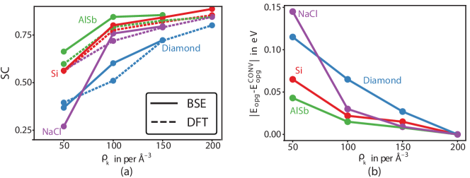
Figure 3: Quantifying the convergence of BSE calculation w.r.t reciprocal density ($\rho_{k}$) through (a) an area similarity coefficient (SC) for spectra and (b) optical gap (E_opg). E${}^{CONV}_{opg}$ is the respective converged value of optical gap for Si (red), Diamond (blue), AlSb (green) and NaCl (purple) based on our calculation. We have shown that the SC computed from DFT (RPA) absorption spectra can be used to check the convergence of BSE calculation w.r.t $\rho_{k}$.

Fig. 3 (a) shows the SC for the spectra of Fig. 2 computed with a $\Delta\rho_{k}$ of 50 per $\mathrm{\AA}^{-3}$. The SC captures both the shifts in peak positions and oscillator strengths in the absorption spectra resulting from the change in reciprocal density used in BSE calculations. As one can see from the absorption spectra of Si and AlSb, Fig.  2(a) and (c), that the peak positions and their oscillator strengths don’t change too much when $\rho_{k}$ is $>$ 100 per $\mathrm{\AA}^{-3}$. This is reflected by a larger value of SC, $>$ 0.75, for them (Fig.  3(a)). Whereas, a lower SC value is obtained for diamond and especially for NaCl even for $\rho_{k}$ is $>$ 100 per $\mathrm{\AA}^{-3}$. This is mostly due to a large change in peak positions for diamond and a change in oscillator strengths for NaCl (Fig.  2(b) and (d)). Nevertheless, once we look at the convergence of SC for both BSE and RPA absorption spectra (Fig.  3(a)), they look quite similar. Thus the lower resource and time-intensive RPA can be employed to estimate the $k$-mesh required to converge the BSE calculations In Fig.  3 (b) we show the convergence of optical gap, $E_{opg}$, with the reciprocal density, $\rho_{k}$, used in BSE calculation. To compare the convergence for these materials that have very different optical gaps we subtracted the converged value of the optical gap, $E^{CONV}_{opg}$, for each of them to show the variation in the same scale. From Fig. 3 (b) it is clear that the $k$-mesh required to obtain an SC $>0.75$ is sufficient to converge the optical gaps within 50 meV for most of the materials. Additionally, Fig. 3(a) indicates that the convergence of the SC ensures that the entire absorption spectra (in the desired frequency range) is also converged along with the optical gap.

3 $py$GWBSE workflow architecture

Figure 4 shows the workflow architecture of $py$GWBSE. The workflow consists of seven fireworks (FW). FWs are a set of tasks, called firetasks (FTs), that together accomplish a specific objective such as DFT structural relaxation. For example, FW1 named SCF is composed of four FTs (see Figure S3 in supplementary information), which enables a DFT simulation by automatically generating the input files, running a simulation on a supercomputing resource, analyzing the simulation output, and storing it in a MongoDB database. Some FWs are optional in the workflow (shown as orange rectangles in Fig 4) while others are essential (shown as purple rectangles in the same figure). Once each of the FWs is completed, the results along with the input parameters necessary to reproduce the results are saved in a MongoDB database.

FWs and FTs were first introduced in the $Fireworks$ jain2015Fireworks open-source package. They allow us to break down and organize a workflow in a group of tasks with the correct order of execution for each task and suitable transfer of information between the tasks. For example, FTs can be simple tasks such as writing files, copying files from a previous directory, or more complex tasks such as starting and monitoring a $VASP$ calculation, or parsing specific information from $VASP$ output files and saving them in a MongoDB database.

$py$GWBSE creates and stores information about FWs, FTs, and their interdependencies in MongoDB database collections as JSON objects. These collections are shown as green cylinders in Fig. 4. At the time of workflow execution on a supercomputer, the FTs of individual FWs are executed in the appropriate order using the JSON objects stored in the MongoDB database. $py$GWBSE workflow needs a file named ‘input.yaml’ to initiate the workflow. In ‘Running the example’ section of supplementary information, we have shown an example ‘input.yaml’ file with a detailed description of all the input tags one need to specify for creating a workflow that demonstrates the capabilities of the $py$GWBSE package.

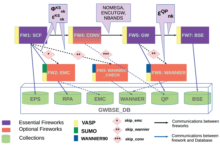
Figure 4: All the FWs, both essential (purple rectangles) and optional (orange rectangles) involved in GW-BSE workflow as implemented in $py$GWBSE code are shown in the flowchart. The input tags that trigger the optional FWs are shown by pink diamonds. The collections that store input parameters and output results from different FWs in the GWBSE database are shown by green cylinders. Essential (solid) and optional (dashed) connections of the FWs with the GWBSE database (blue) and with other FWs (black) are shown with lines. Crucial information communicated between fireworks is shown in light purple callout boxes. Three simulation software $VASP$, $Sumo$ and $Wannier90$ used by the different FWs. They are shown by yellow, green, and blue side bars, respectively, on the individual FWs.

3.1 $py$GWBSE fireworks

As mentioned earlier, we have developed seven FWs in the $py$GWBSE package. They are shown as rectangular boxes in Fig. 4. Each FW is named as shown in the boxes along with an ‘FW’ suffix. The FWs are numbered in order of their execution in the workflow. Three simulation software namely $VASP$, $Sumo$ and $Wannier90$ are used by $py$GWBSE. The software used for individual FWs are denoted by left-sided bars on the FW boxes in Fig. 4.

The first FW, ScfFW, is used to obtain self-consistent charge density by solving the KS equation. It computes KS eigenvalues and wavefunctions, ($\Phi^{KS}_{n\bf k}$ and $\epsilon^{KS}_{n\bf k}$, which are required by all other FWs. Second FW, EmcFW, performs the effective mass calculation (EMC) via the $Sumo$ codeganose2018sumo using the DFT bandstructure obtained by FW1. The third FW, Wannier$\_$checkFW is designed for checking the accuracy of wannier interpolation. Fourth FW, ConvFW performs convergence tests for NBANDS, $ENCUTGW$, and $NOMEGA$ as discussed in Section 2.1.1. Fifth FW, GwFW performs GW calculation to obtain QP energies ($\epsilon^{KS}_{n\bf k}$) as discussed in section 2.1.1 (Eqn. 3 –9). The sixth FW, WannierFW is designed to perform wannier interpolation to obtain QP energies along the high-symmetry k-path to produce GW bandstructure. Lastly, the seventh FW, BseFW solves the Bethe-Salpeter equation to obtain $\epsilon_{2}(\omega)$ as described in Section 2.1.2 (Eqn. 10–13).

The optional FWs are triggered by the input tags described in the pink diamonds. For example, only when $skip\_emc$ tag is set to $False$, the workflow executes EmcFW (FW2) to compute the effective masses. Note that ConvFW (FW4) is labeled as both an essential and optional FW. In the supplementary information (‘Detailed description of $py$GWBSE fireworks’ section) we explain which parts of the FW4 are optional.

Figure S3 in the supplementary information shows the breakdown of each of the 7 FWs of $py$GWBSE workflow into its constituent FTs. There are 4 categories of FTs depending on their functionality. The first category can be considered as file handling FTs (shown as green boxes in Figure S3). These FTs are used to create or copy files. For example, the $WriteVaspFromIOSet$ FT in FW1, FW2, FW3, and FW4 are used to write the INCAR, KPOINTS, POSCAR, and POTCAR input files for the $VASP$ simulations. The second category is that of the simulation FTs (yellow boxes in Figure S3). These FTs launch an executable to run specific simulations on a supercomputer. For example, $Run\_Vasp$ is used to run the $VASP$ software. The third category of FTs, communication FTs (shown in light purple boxes in Figure S3), enables communication between different FTs. For example, $PasscalcLocs$ in FW1 and FW5 is used to pass the address of the directory where a parent FW was executed to its children’s FWs. The last category of FTs, the transfer to database FTs, transfers information to the database. They are shown by gray boxes For example $Eps2db$ in FW1 is used to read dielectric tensor from $VASP$ output file and save it to the database.

We use separate MongoDB collections to store the data and metadata, including inputs and outputs, associated with the FWs and FTs. Fig. 4 shows these various collections. The group of all these collections is called the GWBSE$\_$DB. Dielectric tensors, KS eigenvalues, projections of the KS wavefunctions onto atomic orbitals (for computing projected DOS), RPA dielectric functions from DFT calculation, effective masses, wannier interpolated bandstructures from both DFT and GW levels, all the QP energies including those during convergence, frequency-dependent dielectric function for different light polarization axis from BSE calculations are some of the key quantities stored in the collections.

A more elaborate description of the code’s features and the functionality implementation, especially the convergence of the GW and BSE-related parameters can be found in the ‘Detailed description of $py$GWBSE fireworks’ section of the supplementary information. Moreover, the supplementary information includes an example Jupyter Notebook that shows a step-by-step setup process to create a workflow and analyze the results obtained from the workflow to determine QP properties and the BSE absorption spectra of the wurtzite phase of AlN.

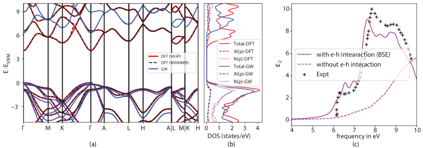
Figure 5: (a) Bandstructure of wurtzite-AlN computed using different methods. DFT bandstructure using direct $VASP$ calculation is shown by red lines and the one obtained from Wannier interpolation is shown as black dashed lines. The QP bandstructure using partial self-consistent GW is shown as blue lines. (b) Total and orbital-resolved DOS for Al (dashed line) and N (dotted line) $p$-states for AlN with both DFT (red) and GW (blue) calculations. (c) Absorption spectra of wurtzite-AlN with (solid) and without (dashed) taking electron-hole interaction into account. The experimental result wethkamp1999dielectric for the same is shown with black ‘$+$’ symbols for comparison.

4 Benchmarking $py$GWBSE for wurtzite AlN

Recently, we employed $py$GWBSE to compute the excitonic effects in absorption spectra of $\sim$ 50 photocatalysts using the Bethe–Salpeter formalism biswas2021excitonic . In that study, we have compared the QP gap computed using $py$GWBSE for 10 materials of very different chemical compositions with the experimental values for the purpose of benchmarking and found excellent agreement. However, in the aforementioned study we haven’t utilized all the functionalities of $py$GWBSE. Therefore, here we demonstrate all the functionalities of the $py$GWBSE workflow by applying it to a test case of wurtzite-AlN. In this section, we compare the various quantities obtained from the workflow simulations with the experimentally measured values reported in the literature.

We begin by evaluating the quantities obtained from the DFT calculations. To that end, the dielectric constants of AlN are found to be $\epsilon_{\infty}^{\perp}$=4.61, $\epsilon_{\infty}^{\parallel}$=4.82 , and $\epsilon^{avg}_{\infty}$= 4.68, with the $\epsilon^{avg}_{\infty}$ being in exact agreement with the experimentally measured value of 4.68 akasaki1967infrared .

The electron effective masses are found to be $m^{\parallel}_{e}$=0.28$m_{0}$ and $m^{\perp}_{e}$=0.3$m_{0}$ which fall in the experimentally obtained ranges of $\sim$ 0.29-0.45$m_{0}$ dreyer2013effects . In case of hole effective masses we find a large anisotropy, $m^{\parallel}_{h}$=0.24$m_{0}$ and $m^{\perp}_{h}$=4.32$m_{0}$. The average hole effective mass in AlN was recently estimated to be $\sim$ 2.7$m_{0}$, based on experimental measurements of the Mg acceptor binding energy in Mg-doped AlN epilayers nam2003mg which is very similar to our average computed value of $m^{avg}_{h}$=2.96.

Fig. 5 (a) shows the bandstructure of AlN computed from DFT using $VASP$ directly (red solid) and through the use of wannier interpolation (black dashed). As one can see that, the wannier interpolation is very accurate and both the bandstructures overlap with each other throughout most of the BZ. Fig. 5 (a) also shows that AlN is a direct gap semiconductor with a DFT gap of 4.05, which is expectedly underestimated compared to the experimental value of 6.2 eV rubio1993quasiparticle but very close to the value obtained from DFT calculations in the earlier studies (3.9 eV)rubio1993quasiparticle .

Once we perform the one-shot GW calculation the direct gap increases to 5.59 eV. Although this is closer to the experimental value it is still not quite accurate. Previous studies, using an LDA functional as a starting point found a QP gap of 5.8 eV, which also doesn’t agree with the experimental gap. However, after we perform partial self-consistent GW (scGW) the QP gap becomes 6.28 eV, resulting in an excellent agreement with the experimental value of 6.2 eV rubio1993quasiparticle . The QP bandstructure with scGW is shown by the blue curve in Fig. 5 (a).

We use the QP energies and projection of KS wavefunctions or atomic orbitals to compute the orbital resolved DOS with QP corrections under the assumption that the KS wavefunction is a good approximation for the QP wavefunction. Fig. 5 (b) shows the orbital-resolved DOS of wurtzite-AlN with Al($p$) and N($p$) states shown with dashed and dotted lines respectively. We show orbital-resolved DOS obtained from both DFT and GW calculations for comparison. Our calculation suggests that the valence band edge of wurtzite-AlN mostly consists of N($p$) states, whereas the conduction band edge is resulting from strong hybridization between Al($p$) and N($p$) states, which is consistent with the findings of previous studies jiao2011comparison .

To show $py$GWBSE’s ability to perform BSE calculation and obtain absorption spectra ($\epsilon_{2}(\omega)$) that include electron-hole interactions we perform the GW-BSE calculation for wurtzite-AlN. Fig. 5 (c) compares the absorption spectra ($\epsilon_{2}(\omega)$) that we obtained from the BSE calculation, the calculation without electron-hole interaction, and the experimentally obtained spectra from the literature wethkamp1999dielectric . The light polarization is set to be perpendicular to the $c$-axis. As we can see from Fig. 5 (c) the absorption spectra calculated without taking electron-hole (e-h) interaction into account completely misses the features in the 6–10 eV range, visible in the experimental absorption spectra (shown with ‘$+$’ symbols in Fig. 5 (c). Only when we include the e-h interaction through the BSE calculation those excitonic features are retrieved. Although, the absorption spectra obtained from BSE very closely resemble the experimental absorption spectra we find that the sharp absorption edge at 6.2 eV and two prominent absorption peaks at 7.85 and 8.95 eV are shifted (by $\sim$ 0.15 eV for the peaks) to the lower frequencies. We have used a $\rho_{k}$ value of 200 per $\mathrm{\AA^{-3}}$ (12$\times$12$\times$7 $k$-grid) with a broadening ($CSHIFT$) VASP of 0.2 eV for our AlN BSE calculation, which produces an SC value of 0.89 (see Fig. S4 in supplementary information for convergence results). In the figures in the SI, we can see that with an SC of $\sim$ 0.75 reasonable amount of information is obtained for the spectra peaks and their positions, however, clearly larger SC’s lead to better accuracy, albeit at a higher computational cost and computing time. Thus previous GW-BSE calculations with a finer sampling of the BZ, with randomly distributed 1000 $k$-points, led to even better agreement with the experimental spectra.bechstedt2005quasiparticle

5 Conclusion

We have developed a Python toolkit, $py$GWBSE, which enables high-throughput GW-BSE calculations. In this article, we present the underlying theory, the workflow architecture, the algorithmic implementation, and benchmark simulations for the $py$GWBSE code. This open-source code (available at ${\it https://github.com/cmdlab/pyGWBSE}$) enables automated input file generation, submission to supercomputing platforms, analysis of post-simulation data, and storage of metadata and data in a MongoDB database. Moreover, $py$GWBSE is capable of handling multiple convergence parameters associated with the GW-BSE formalism. To reduce the computational cost associated with obtaining a converged absorption spectrum from BSE calculations, we present a novel strategy for computing the similarity coefficient from RPA spectra. We have shown that this approach ensures convergence of not only the optical gap or exciton binding energy but the entire absorption spectra in the desired frequency range. Our openly available code will help to include QP properties and excitonic effects in future computational material design and discovery studies in a variety of fields such as power electronics, photovoltaics, and photocatalysis. The $py$GWBSE will facilitate high-throughput GW-BSE simulations enabling the application of large data methods to further explore our understanding of materials as well as first-principles methods that are designed for computing excited state properties.

6 Acknowledgements

This work was supported by ULTRA, an Energy Frontier Research Center funded by the U.S. Department of Energy (DOE), Office of Science, Basic Energy Sciences (BES), under Award $\#$ DE-SC0021230. In addition, Singh acknowledges support by the Arizona State University start-up funds. The authors acknowledge the San Diego Supercomputer Center under the NSF-XSEDE Award No. DMR150006 and the Research Computing at Arizona State University for providing HPC resources. This research used resources of the National Energy Research Scientific Computing Center, a DOE Office of Science User Facility supported by the Office of Science of the U.S. Department of Energy under Contract No. DE-AC02-05CH11231. The authors also thank Tara M. Boland, Adway Gupta, Akash Patel, and Cody Milne for testing of the code and helpful discussions.

References

- \bibcommenthead
- (1) Singh, A.K., Montoya, J.H., Gregoire, J.M., Persson, K.A.: Robust and synthesizable photocatalysts for reduction: a data-driven materials discovery. Nature communications 10(1), 1–9 (2019)
- (2) Wu, Y., Lazic, P., Hautier, G., Persson, K., Ceder, G.: First principles high throughput screening of oxynitrides for water-splitting photocatalysts. Energy & environmental science 6(1), 157–168 (2013)
- (3) Kirklin, S., Meredig, B., Wolverton, C.: High-throughput computational screening of new li-ion battery anode materials. Advanced Energy Materials 3(2), 252–262 (2013)
- (4) Hautier, G., Jain, A., Ong, S.P., Kang, B., Moore, C., Doe, R., Ceder, G.: Phosphates as lithium-ion battery cathodes: an evaluation based on high-throughput ab initio calculations. Chemistry of Materials 23(15), 3495–3508 (2011)
- (5) Choudhary, K., Garrity, K.F., Sharma, V., Biacchi, A.J., Hight Walker, A.R., Tavazza, F.: High-throughput density functional perturbation theory and machine learning predictions of infrared, piezoelectric, and dielectric responses. NPJ Computational Materials 6(1), 1–13 (2020)
- (6) Greeley, J., Jaramillo, T.F., Bonde, J., Chorkendorff, I., Nørskov, J.K.: Computational high-throughput screening of electrocatalytic materials for hydrogen evolution. Nature materials 5(11), 909–913 (2006)
- (7) Jones, R.O.: Density functional theory: Its origins, rise to prominence, and future. Reviews of modern physics 87(3), 897 (2015)
- (8) Perdew, J.P.: Density functional theory and the band gap problem. International Journal of Quantum Chemistry 28(S19), 497–523 (1985)
- (9) Hedin, L.: New method for calculating the one-particle green’s function with application to the electron-gas problem. Physical Review 139(3A), 796 (1965)
- (10) Onida, G., Reining, L., Rubio, A.: Electronic excitations: density-functional versus many-body green’s-function approaches. Reviews of modern physics 74(2), 601 (2002)
- (11) Muscat, J., Wander, A., Harrison, N.: On the prediction of band gaps from hybrid functional theory. Chemical Physics Letters 342(3-4), 397–401 (2001)
- (12) Vines, F., Lamiel-García, O., Chul Ko, K., Yong Lee, J., Illas, F.: Systematic study of the effect of hse functional internal parameters on the electronic structure and band gap of a representative set of metal oxides. Journal of computational chemistry 38(11), 781–789 (2017)
- (13) Kotani, T., Van Schilfgaarde, M.: Impact ionization rates for si, gaas, inas, zns, and gan in the g w approximation. Physical Review B 81(12), 125201 (2010)
- (14) Darancet, P., Ferretti, A., Mayou, D., Olevano, V.: Ab initio g w electron-electron interaction effects in quantum transport. Physical Review B 75(7), 075102 (2007)
- (15) Rangel, T., Ferretti, A., Trevisanutto, P., Olevano, V., Rignanese, G.-M.: Transport properties of molecular junctions from many-body perturbation theory. Physical Review B 84(4), 045426 (2011)
- (16) Biswas, T., Jain, M.: Electronic structure and optical properties of f centers in -alumina. Physical Review B 99(14), 144102 (2019)
- (17) Freysoldt, C., Grabowski, B., Hickel, T., Neugebauer, J., Kresse, G., Janotti, A., Van de Walle, C.G.: First-principles calculations for point defects in solids. Reviews of modern physics 86(1), 253 (2014)
- (18) Kioupakis, E., Rinke, P., Delaney, K.T., Van de Walle, C.G.: Indirect auger recombination as a cause of efficiency droop in nitride light-emitting diodes. Applied Physics Letters 98(16), 161107 (2011)
- (19) McAllister, A., Åberg, D., Schleife, A., Kioupakis, E.: Auger recombination in sodium-iodide scintillators from first principles. Applied Physics Letters 106(14), 141901 (2015)
- (20) Ugeda, M.M., Bradley, A.J., Shi, S.-F., Felipe, H., Zhang, Y., Qiu, D.Y., Ruan, W., Mo, S.-K., Hussain, Z., Shen, Z.-X., et al.: Giant bandgap renormalization and excitonic effects in a monolayer transition metal dichalcogenide semiconductor. Nature materials 13(12), 1091–1095 (2014)
- (21) Rohlfing, M., Louie, S.G.: Electron-hole excitations and optical spectra from first principles. Physical Review B 62(8), 4927 (2000)
- (22) Hafner, J.: Ab-initio simulations of materials using vasp: Density-functional theory and beyond. Journal of computational chemistry 29(13), 2044–2078 (2008)
- (23) Ong, S.P., Richards, W.D., Jain, A., Hautier, G., Kocher, M., Cholia, S., Gunter, D., Chevrier, V.L., Persson, K.A., Ceder, G.: Python materials genomics (pymatgen): A robust, open-source python library for materials analysis. Computational Materials Science 68, 314–319 (2013)
- (24) Jain, A., Ong, S.P., Chen, W., Medasani, B., Qu, X., Kocher, M., Brafman, M., Petretto, G., Rignanese, G.-M., Hautier, G., et al.: Fireworks: A dynamic workflow system designed for high-throughput applications. Concurrency and Computation: Practice and Experience 27(17), 5037–5059 (2015)
- (25) Mathew, K., Montoya, J.H., Faghaninia, A., Dwarakanath, S., Aykol, M., Tang, H., Chu, I.-h., Smidt, T., Bocklund, B., Horton, M., et al.: Atomate: A high-level interface to generate, execute, and analyze computational materials science workflows. Computational Materials Science 139, 140–152 (2017)
- (26) Mostofi, A.A., Yates, J.R., Lee, Y.-S., Souza, I., Vanderbilt, D., Marzari, N.: wannier90: A tool for obtaining maximally-localised wannier functions. Computer physics communications 178(9), 685–699 (2008)
- (27) Blöchl, P.E.: Projector augmented-wave method. Physical review B 50(24), 17953 (1994)
- (28) Singh, D.: Planes Waves, Pseudopotentials and the LAPW. Method, Kluwer Academic (1994)
- (29) Leng, X., Jin, F., Wei, M., Ma, Y.: Gw method and bethe–salpeter equation for calculating electronic excitations. Wiley Interdisciplinary Reviews: Computational Molecular Science 6(5), 532–550 (2016)
- (30) Faber, C., Boulanger, P., Attaccalite, C., Duchemin, I., Blase, X.: Excited states properties of organic molecules: From density functional theory to the gw and bethe–salpeter green’s function formalisms. Philosophical Transactions of the Royal Society A: Mathematical, Physical and Engineering Sciences 372(2011), 20130271 (2014)
- (31) Blase, X., Duchemin, I., Jacquemin, D.: The bethe–salpeter equation in chemistry: relations with td-dft, applications and challenges. Chemical Society Reviews 47(3), 1022–1043 (2018)
- (32) Jain, A., Hautier, G., Moore, C.J., Ong, S.P., Fischer, C.C., Mueller, T., Persson, K.A., Ceder, G.: A high-throughput infrastructure for density functional theory calculations. Computational Materials Science 50(8), 2295–2310 (2011)
- (33) Kresse, G., Marsman, M.: J. Furthmüller VASP the GUIDE (2018)
- (34) Hybertsen, M.S., Louie, S.G.: Electron correlation in semiconductors and insulators: Band gaps and quasiparticle energies. Physical Review B 34(8), 5390 (1986)
- (35) Shishkin, M., Kresse, G.: Implementation and performance of the frequency-dependent method within the framework. Physical Review B 74(3), 035101 (2006)
- (36) Hybertsen, M.S., Louie, S.G.: Ab initio static dielectric matrices from the density-functional approach. i. formulation and application to semiconductors and insulators. Physical Review B 35(11), 5585 (1987)
- (37) Shishkin, M., Kresse, G.: Self-consistent calculations for semiconductors and insulators. Physical Review B 75(23), 235102 (2007)
- (38) Delaney, K., García-González, P., Rubio, A., Rinke, P., Godby, R.W.: Comment on “band-gap problem in semiconductors revisited: effects of core states and many-body self-consistency”. Physical review letters 93(24), 249701 (2004)
- (39) Schöne, W.-D., Eguiluz, A.G.: Self-consistent calculations of quasiparticle states in metals and semiconductors. Physical review letters 81(8), 1662 (1998)
- (40) Tiago, M.L., Ismail-Beigi, S., Louie, S.G.: Effect of semicore orbitals on the electronic band gaps of si, ge, and gaas within the gw approximation. Physical Review B 69(12), 125212 (2004)
- (41) Deslippe, J., Samsonidze, G., Jain, M., Cohen, M.L., Louie, S.G.: Coulomb-hole summations and energies for g w calculations with limited number of empty orbitals: A modified static remainder approach. Physical Review B 87(16), 165124 (2013)
- (42) Strinati, G.: Application of the green’s functions method to the study of the optical properties of semiconductors. La Rivista del Nuovo Cimento (1978-1999) 11(12), 1–86 (1988)
- (43) Kammerlander, D., Botti, S., Marques, M.A., Marini, A., Attaccalite, C.: Speeding up the solution of the bethe-salpeter equation by a double-grid method and wannier interpolation. Physical Review B 86(12), 125203 (2012)
- (44) Jekel, C.F., Venter, G., Venter, M.P., Stander, N., Haftka, R.T.: Similarity measures for identifying material parameters from hysteresis loops using inverse analysis. International Journal of Material Forming 12(3), 355–378 (2019)
- (45) Ganose, A., Jackson, A., Scanlon, D.: sumo: Command-line tools for plotting and analysis of periodic* ab initio* calculations. Journal of Open Source Software 3(28), 717 (2018)
- (46) Wethkamp, T., Wilmers, K., Cobet, C., Esser, N., Richter, W., Ambacher, O., Stutzmann, M., Cardona, M.: Dielectric function of hexagonal aln films determined by spectroscopic ellipsometry in the vacuum-uv spectral range. Physical Review B 59(3), 1845 (1999)
- (47) Biswas, T., Singh, A.K.: Excitonic effects in absorption spectra of carbon dioxide reduction photocatalysts. npj Computational Materials 7(1), 1–10 (2021)
- (48) Akasaki, I., Hashimoto, M.: Infrared lattice vibration of vapour-grown aln. Solid State Communications 5(11), 851–853 (1967)
- (49) Dreyer, C., Janotti, A., Van de Walle, C.: Effects of strain on the electron effective mass in gan and aln. Applied Physics Letters 102(14), 142105 (2013)
- (50) Nam, K., Nakarmi, M., Li, J., Lin, J., Jiang, H.: Mg acceptor level in aln probed by deep ultraviolet photoluminescence. Applied physics letters 83(5), 878–880 (2003)
- (51) Rubio, A., Corkill, J.L., Cohen, M.L., Shirley, E.L., Louie, S.G.: Quasiparticle band structure of aln and gan. Physical review B 48(16), 11810 (1993)
- (52) Jiao, Z.-Y., Ma, S.-H., Yang, J.-F.: A comparison of the electronic and optical properties of zinc-blende, rocksalt and wurtzite aln: A dft study. Solid State Sciences 13(2), 331–336 (2011)
- (53) The VASP Manual. https://www.vasp.at/wiki/index.php/The_VASP_Manual
- (54) Bechstedt, F., Seino, K., Hahn, P., Schmidt, W.: Quasiparticle bands and optical spectra of highly ionic crystals: Aln and nacl. Physical Review B 72(24), 245114 (2005)