Multi-Robot Motion Planning for Unit Discs with Revolving Areas††thanks: Work by Pankaj K. Agarwal and Erin Taylor is supported by IIS-1814493, CCF-2007556, and CCF-2223870. Work by Dan Halperin and Tzvika Geft has been supported in part by the Israel Science Foundation (grant no. 1736/19), by NSF/US-Israel-BSF (grant no. 2019754), by the Israel Ministry of Science and Technology (grant no. 103129), by the Blavatnik Computer Science Research Fund, and by the Yandex Machine Learning Initiative for Machine Learning at Tel Aviv University. Tzvika Geft has also been supported by a scholarship from the Shlomo Shmeltzer Institute for Smart Transportation at Tel Aviv University.
Abstract
We study the problem of motion planning for a collection of labeled unit disc robots in a polygonal environment. We assume that the robots have revolving areas around their start and final positions: that each start and each final is contained in a radius disc lying in the free space, not necessarily concentric with the start or final position, which is free from other start or final positions. This assumption allows a weakly-monotone motion plan, in which robots move according to an ordering as follows: during the turn of a robot in the ordering, it moves fully from its start to final position, while other robots do not leave their revolving areas. As passes through a revolving area, a robot that is inside this area may move within the revolving area to avoid a collision. Notwithstanding the existence of a motion plan, we show that minimizing the total traveled distance in this setting, specifically even when the motion plan is restricted to be weakly-monotone, is APX-hard, ruling out any polynomial-time -approximation algorithm.
On the positive side, we present the first constant-factor approximation algorithm for computing a feasible weakly-monotone motion plan. The total distance traveled by the robots is within an factor of that of the optimal motion plan, which need not be weakly monotone. Our algorithm extends to an online setting in which the polygonal environment is fixed but the initial and final positions of robots are specified in an online manner. Finally, we observe that the overhead in the overall cost that we add while editing the paths to avoid robot-robot collision can vary significantly depending on the ordering we chose. Finding the best ordering in this respect is known to be NP-hard, and we provide a polynomial time -approximation algorithm for this problem.
1 Introduction
Multi-robot systems are already in use in logistics, in a variety of civil engineering and nature preserving tasks, and in agriculture, to name a few areas. They are anticipated to proliferate in the coming years, and accordingly they attract intensive research efforts in diverse communities.
A basic motion-planning problem for a team of robots is to plan such collision-free paths for the robots between given start and final positions. Among the many dimensions along which the multi-robot motion planning (MRMP) problem has been studied, we focus on three: (1) we distinguish between distributed and centralized control. In the former each robot has limited knowledge of the entire environment where the robots move, and each robot may communicate with few neighboring robots. In the latter, which is typical in factory automation and other well-structured environments, a central authority has control over all the robots and the planning for each robot takes into consideration knowledge about the state of all the other robots in the system. (2) In the labeled version the robots are distinguishable from one another and each robot has its own assigned target, whereas in the unlabeled version the robots are indistinguishable, i.e., each target can be occupied by any robot in the team and the motion-planning problem is considered solved if at the end of the motion all the target positions are occupied. (3) We further distinguish between continuous or discrete domains. Much of the study of motion planning in computational geometry and robotics assumes that the workspace is continuous. In AI research, where the problem is typically called multi-agent path finding (MAPF) [21], the domain is modeled as a graph. Nowadays the MAPF problem is studied in diverse research communities, often as an approximation of the continuous domain.
In our study here we consider a centralized, labeled, and continuous version of MRMP. Furthermore, we are not only interested in finding a solution to the given motion-planning problem, but rather in finding a high-quality solution. Specifically, we aim to find a solution that minimizes the total path length traveled by the robots.
Related Work.
Computing a feasible motion plan (not necessarily a good one) itself is in general computationally hard for MRMP (see, e.g., [11, 4, 18, 9]). In the results that we cite next, some additional mitigating conditions are assumed on the system to obtain efficient motion-planning algorithms.
There are few results that guarantee bounds on the quality of the motion plans for multi-robot systems. For complete algorithms111A motion planning algorithm is called complete if, in finite time, it is guaranteed to find a solution or determine that no solution exists. in the unlabeled case, there are bounds on the length of the longest path taken by a robot in the system [22], or on the sum of distance traveled by all the robots [20]. For the labeled case, Demaine et al. [7] provide constant-factor approximation algorithms for minimizing the execution time of a coordinated parallel motion if there are no obstacles. Still for the labeled case, Solomon and Halperin obtained a very crude bound on the sum of distances [17] (the approximation factor can be linear in the complexity of the environment in the worst case) in a setting identical to the setting of the current paper, namely assuming the existence of revolving areas—see below for a formal definition. No sublinear approximation algorithm is known for MRMP even if we assume the existence of revolving areas and the cost of a motion plan is the sum of the lengths of individual paths. In the current paper we significantly improve over and expand the results in [17] in several ways, as we discuss below.
An alternative approach to cope with the hardness of motion planning is to use sampling-based methods [14]. In their seminal paper, Karaman and Frazzoli [12] (see also [19]) introduced an algorithm, called RRT*, which guarantees near optimality if the number of samples tends to infinity. A related algorithm dRRT* handles the multi-robot case with the same type of guarantee [16]. Recently Dayan et al. [6] have obtained near-optimality with finite sample size for the multi-robot case.
Problem Statement.
Let be a polygonal environment, that is, a polygon with holes in and a total of vertices. Let be robots, each modeled as a unit disc, that move around in . Let be the obstacle space. For a point , let denote the unit disc centered at point . Let represent the free space of (with respect to one ). A path is a continuous function from an interval to , and is collision-free if it is contained in . Let denote the arc length of , i.e., . The position of each is specified by the - and -coordinates of its center and we use to denote being at (note that is the same as ), and a motion of is specified by the path followed by its center. Let denote the interior of disc . A path ensemble is a set of paths defined over a common interval , i.e. , for ; is called feasible if (i) for every , and (ii) for any and for any pair , , i.e., the ’s remain in and they do not collide with each other (but may touch each other) during the entire motion. We also refer to as a motion plan of . The cost of , denoted by , is defined as .
We are given a set of start positions where the robots initially lie and a set of final (also called target) positions . Our goal is to find a path ensemble over an interval where denotes the ending time of the last robot movement,
- (i)
-
and for all , and
- (ii)
-
where the minimum is taken over all feasible path ensembles.
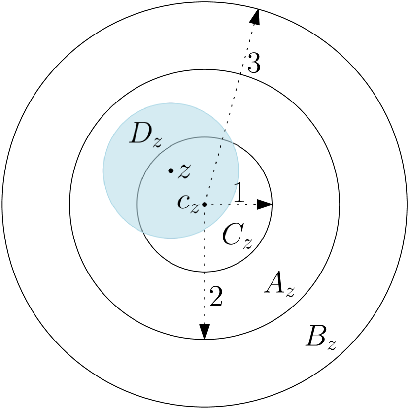
We refer to the problem as optimal multi-robot motion planning (MRMP). In this paper, we investigate optimal MRMP under the assumption that there is some free space around the starting and final positions of , a formulation introduced in [17]. A revolving area of a start or final position , is a disc of radius such that: (i) , (ii) , and (iii) for any other start or final position , . That is, each lies in a revolving area at its start and final position (note that need not be the center of the revolving area and does not intersect any other revolving areas, and the revolving areas do not intersect any obstacles. We remark that the revolving areas may intersect one another; this makes the separation assumptions in the current paper lighter than in related results (e.g.,[1]), which in turn makes the analysis more involved. See Figure 1 for an example. Set . We refer to this problem as optimal multi-robot motion planning with Revolving Areas (MRMP-RA).
We define the active interval as the open interval from the first time leaves the revolving area of to the last time is not in the revolving area of . If the active intervals are pairwise disjoint then we call a weakly-monotone motion plan (with respect to revolving areas).222We use the term “weakly-monotone” because a plan is called monotone if the active interval of is defined from when leaves for the first time until reaches for the last time, (rather than the leaving/reaching the revolving area /). Finally, an instance of optimal MRMP is specified as where are as defined above. Let denote an optimal solution of and let .
Our Results.
The paper contains the following three main results:
- (A) Hardness results.
-
In Section 2, we show that MRMP-RA is NP-hard under the weakly-monotone assumption. The NP-hardness of optimizing sum of distances (i.e., optimal MRMP) for the monotone and the general (non-monotone) case was shown in [10], but without revolving areas. Our main result here is the extension of the NP-hardness construction to prove that MRMP-RA, under the weakly-monotone assumption, is in fact APX-hard, which rules out a polynomial-time -approximation algorithm for it. To the best of our knowledge, this is the first APX-hardness result for any MRMP variant.
- (B) Approximation algorithm.
-
In Section 3, we present the first -approximation algorithm that given an instance of MRMP-RA computes a feasible path ensemble from to such that is weakly-monotone and ; note that need not be weakly-monotone, i.e., we approximate the general optimal path ensemble. In fact, we show that the robots can be moved in any order, so our algorithm can be extended to an online setting where the robots , and their start/final positions, are given in an online manner, or ’s may have to execute multiple tasks which are given in an online manner– the so-called life-long planning problem. Our algorithm ensures an competitive ratio, i.e., the cost is times the optimal cost of the offline problem.
The algorithm begins by computing a set of shortest paths that avoid obstacles but ignore robot-robot collisions. Then, is edited to avoid robot-robot collisions by moving non-active robots within their revolving areas. Our overall approach is the same as by Solomon and Halperin [17], but the editing of differs significantly from [17], so that the cost of the paths does not increase by too much. We use a more conservative editing of , which enables us to prove that the cost of the edited path ensemble is (see Section 4), while the cost of the edited path in [17] is333Notice that the roles of and here are reversed with respect to [17]. . Our main technical contributions are defining a more conservative retraction, proving that the motion plan remains feasible even under this conservative retraction, and bounding the total cost of the motion plan by using a combination of local and global arguments. Analyzing both the feasibility and the cost of the motion plan are nontrivial and require new ideas.
- (C) Computing a good ordering.
-
The result above shows that editing the paths increases the total cost of the motion plan only by a constant factor irrespective of the order in which we move the robots. However, the overhead in the overall cost due to editing (to avoid robot-robot collisions) can vary significantly depending on the ordering we chose. This raises the question whether we can find a “good" ordering that minimizes the overhead. The result in [17] implies that the problem of finding a good ordering that minimizes the amount of overhead is NP-hard.444The model in [17] for defining the overhead is different from ours, their construction can nevertheless be adapted to our setting. We present a polynomial time -approximation algorithm for finding a good ordering. This is achieved by reducing the problem to an instance of weighted feedback arc set in a directed graph, and applying an approximation algorithm for the latter problem [8]. Due to lack of space, this result is described in Section 5.
We emphasize that without additional, mitigating, assumptions, MRMP is intractable. Sampling-based planners assume that the full solution paths have some clearance around them—namely, each robot has some distance from the obstacles along its entire path, as well as from the other robots. Here, we assume certain clearance only at the start and goal positions; we do not make any assumption about the clearance along the paths. Indeed, we assume non-negligible clearance, as we require that each robot at a start or goal position is encapsulated inside a disc of radius , which does not contain any other robot at its start or goal position. The choice of the number here is not arbitrary. In a couple of related results for MRMP of unit discs [1, 2] this is the critical value of clearance below which there does not always exist a solution to the problem.
2 Hardness of Distance Optimal MRMP-RA
In this section we present our hardness results. Throughout this section all path ensembles are weakly-monotone, unless otherwise stated. With a slight abuse of notation we use to denote the cost of the optimal weakly-monotone path ensemble. Finding monotone path ensembles has been shown to be NP-hard in [9] using a similar grid-based construction without revolving areas.
NP-Hardness of weakly-monotone MRMP-RA
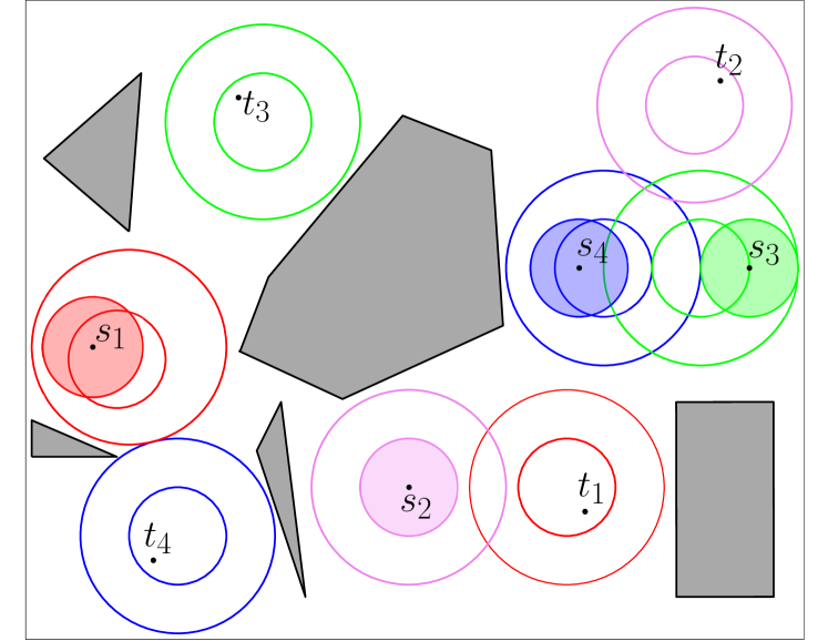
Let be an instance of 3SAT with variables and clauses. Each clause is a disjunction of three literals, which are variables or their negations. We construct a corresponding MRMP-RA instance with robots and choose a real value such that if and only if is satisfiable. Let , where is the length of the optimal path of from to in , ignoring other robots. In fact, our construction will choose to be , that is, is the lowest possible cost of a feasible path ensemble from to in . Our construction will ensure that the lowest cost is attained if and only if is satisfiable. is constructed so that a path ensemble with such a cost is possible if and only if (a feasible) monotone motion plan exists. An example of the construction is shown in Figure 2.
Overall description. The workspace consists of rectangular gadgets, one for each variable and each clause, referred to as variable and clause gadgets, respectively. All the gadgets have unit-width passages that are wider around revolving areas. For simplicity, the widened areas are shown as circular arcs, but they can easily be made polygonal. Each gadget has an entrance on the left and an exit on the right. The vertical positions of entrances and exits alternate so that a gadget’s entrance is connected to the exit of the gadget on its left.
There are robots, each being a unit disc: one robot for each appearance of a literal in , which are collectively called literal robots, and one special pivot robot (shown in blue in Figure 2). The robot has to pass through all the gadgets from left to right, by which it is able to verify the satisfiability of , and the literal robots will constrain its motion in order to ensure that .
Each variable (resp.clause) gadget contains two (resp. three) horizontal passages, which offer two (resp. three) shortest paths from its entrance to its exit. Each such path consists of vertical and horizontal line segments. The horizontal passages of the gadgets contain all the start and target positions of literal robots. All the revolving areas are centered at their respective start or target positions, and they do not overlap.
Gadgets. Each variable gadget initially contains robots representing literals of a single variable of . The top and bottom horizontal passages of the gadget contain robots representing only positive and negative literals, respectively. Each clause gadget has three horizontal passages, each containing a target position of one the literals in the corresponding clause. The gadgets are placed within a horizontal strip from left to right such that variable gadgets are located to the left of clause gadgets. The order of gadgets of the same type is arbitrary, however it determines the order of the start positions, which is critical: the left to right order of start positions within each variable gadget is set to match the left to right order of the corresponding target positions. We refer to this order as the intra-literal order property. We say that a revolving area is congested if it contains two robots at the same time. Intuitively, both optimal path ensembles and monotone path ensembles need to prevent revolving areas from becoming congested. We first establish that finding an optimal weakly-monotone path ensemble is equivalent to finding a monotone one, then show the equivalence between a satisfying assignment and a monotone path ensemble.
Lemma 1.
has a weakly monotone path ensemble with a cost of if and only if has a monotone path ensemble.
Proof.
Let be a revolving area in . We first note that without any loss of generality, in any path ensemble of a robot may either be contained in at some point or never intersect at all. That is, a robot will not partially penetrate a revolving area without ever fully entering it. Let be a feasible path ensemble with . We fix a robot and examine the motion that occurs during its active interval . We claim that any motion of a robot during is redundant, i.e., if does not move during then can still perform the same motion. This suffices in order to conclude that can be made monotone. Observe that during the execution of no revolving area can become congested, as otherwise the two robots that are simultaneously in will have to take a path that is longer than the shortest path that ignores other robots. Therefore, whenever is inside a revolving area , it is the only robot in , and any motion by other robots is redundant. Whenever is not contained in any revolving area, all other robots must be contained in revolving areas, by definition. Hence, any motion by other robots at such point in time is also redundant. So overall, may travel along its whole path without other robots moving. For the other direction, in a monotone path ensemble it also holds that no revolving area may become congested (as otherwise robots move simultaneously). Therefore, any revolving area that some robot intersects during its motion must not contain other robots. For any gadget that needs to traverse, this allows to take some shortest path through . Therefore, is able to take the shortest path that ignores other robots overall. Hence, a path ensemble with a cost of exists. ∎
Lemma 2.
has a satisfying assignment if and only if has a monotone path ensemble.
Proof.
Assume that has a satisfying assignment . Let (resp. ) denote the set of robots corresponding to literals that evaluate to true (resp. false) according to . That is, for each variable gadget, contains robots that are all initially either in the top or the bottom passage, according to . We show that the robots can move along optimal paths in the order , , , which is made precise below.
Let be a shortest collision-free path from to that passes only through the start positions of and targets of ; see Figure 2. The path exists because each clause gadget must contain a target of some robot in , or else does not satisfy .
In the path ensemble, each follows the subpath of from (through which passes) up to the gadget containing , from which can reach its final position using the shortest path. The order in which the robots in move is the right to left order of their start positions, which guarantees no collision with another robot located at its start position. Since the robots in move before , the targets through which passes are unoccupied when the robots in move, guaranteeing no collisions at clause gadgets. Next, moves using , which passes through empty passages at this point. Finally, each joins at the vertical passage to its right, from which point it continues similarly to . The order of motion of the robots in is the right to left order of their targets, which guarantees no collisions in the clause gadgets. Note that due to the intra-literal order property we also have no interferences among within variable gadgets.
For the other direction, let us assume that there is a monotone path ensemble for . Let denote the path taken by . Without loss of generality, is weakly -monotone. Specifically, it passes through only one horizontal passage in each variable gadget. Therefore, we define an assignment as follows: is assigned to be true if and only if goes through the bottom passage of ’s variable gadget, which corresponds to negative literals. Let be a clause of and let be a target in ’s clause gadget that is unoccupied during ’s motion, which must exist. It is easy to verify that the literal corresponding to is true according to . Therefore, is satisfied. ∎
The construction can be carried out in polynomial time, therefore by combining Lemma 1 and Lemma 2 we obtain the following:
Theorem 3.
MRMP-RA for weakly-monotone path ensembles is NP-hard.
Hardness of Approximation
We now show that MRMP-RA is APX-hard, ruling out any polynomial time -approximation algorithm. We first go over some definitions. For an MRMP-RA instance , we use to denote the cost of the optimal weakly-monotone path ensemble for . For a 3SAT formula , let denote the largest fraction of clauses in that can be simultaneously satisfied. We say that a revolving area is occupied if it contains the robot whose start or target position lies in .
To prove the hardness of approximation we present a gap-preserving reduction from MAX-3SAT(5), which is APX-hard [23]. The input to MAX-3SAT(5) is a 3SAT formula with 5 appearances for each variable and the goal is to find an assignment maximizing the number of satisfied clauses. Let be a MAX-3SAT(5) instance with variables and clauses and let be the MRMP-RA instance resulting from the NP-Hardness reduction described above, which we slightly modify as follows. Instead of the single pivot robot in , we now have pivot robots. To this end, we modify the construction so that there is a horizontal passage that extends to the left of in . The passage is lengthened to accommodate start positions that lie on the same horizontal line, passing through in . Similarly, another such passage is created to the right of to accommodate target positions. The left to right order of the start positions of the pivot robots is set to match the left to right order of the corresponding target positions. Let denote the resulting MRMP-RA instance.
Lemma 4.
Let be a 3SAT formula such that for any assignment to there are at least unsatisfied clauses in . Then .
Proof.
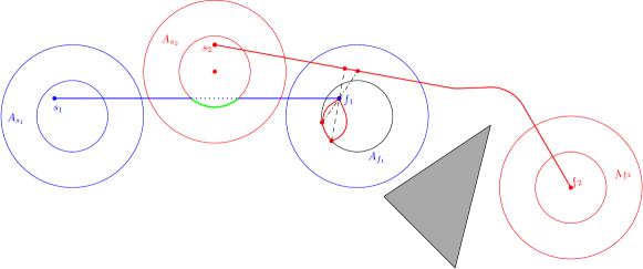
Let us examine , an optimal path ensemble for . We say that a robot has a bad event during the execution of when traverses an occupied revolving area. Note that each bad event results in having a path longer than 1+, being the length of ’s shortest possible path. We claim that each of the pivot robots has bad events, which suffices for proving the lemma.
Let us assume for a contradiction that one of the pivot robots, say , has bad events. We will show how to obtain an assignment for where there are at most unsatisfied clauses. Since is optimal, , the path taken by , is weakly -monotone. We define an assignment as follows (the same way as in the second direction of the proof of Theorem 2): is assigned to be true if and only if goes through the bottom passage of ’s variable gadget. In other words, sets a literal to be true if and only if the corresponding literal-robot’s starting position does not lie on . Let us examine right before it is ’s turn to move. Let denote the set of robots that are intersected by and are located at variable gadgets at this point in time. We can assume without any loss of generality that is empty. If it is not, then let us examine the path ensemble where the robots in move to their targets before ’s turn. The number of bad events for can only decrease in . This holds because by having some move before we eliminate a bad event (for ) in ’s variable gadget and possibly introduce a bad event in ’s clause gadget.
Since there are bad events for , there are at most clause gadgets where such an event occurs. Therefore, to get a contradiction it suffices to show that all other clause gadgets correspond to clauses that are satisfied by . Let be such a clause, i.e., in the corresponding clause gadget passes through some empty revolving area . Since does not pass through any occupied revolving areas in the variable gadgets, the corresponding start position must not lie on . Therefore, corresponds to a literal that is true by , and so is satisfied. ∎
We now make explicit using an upper bound for an arbitrary . First, we bound the length of each vertical segment in the corresponding path by 10, which provides sufficient distance for our gadgets. Since each variable appears in five times, we bound the horizontal length of an variable gadget by (i.e., there at most 4 revolving areas on a horizontal passage and some additional length). Therefore, the path length through any gadget is . Hence, we have and the number of robots is also (we have ). Therefore, we can set for some sufficiently large constant (we can easily lengthen paths in if that is needed for the bound). We can now combine the latter equality with Lemma 4 and the NP-Hardness reduction. Let us define .
Theorem 5.
There is a polynomial time reduction that transforms an instance of MAX-3SAT(5) with clauses to an MRMP-RA instance such that for some constant and otherwise .
3 Algorithm
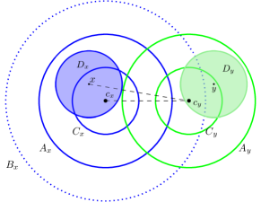
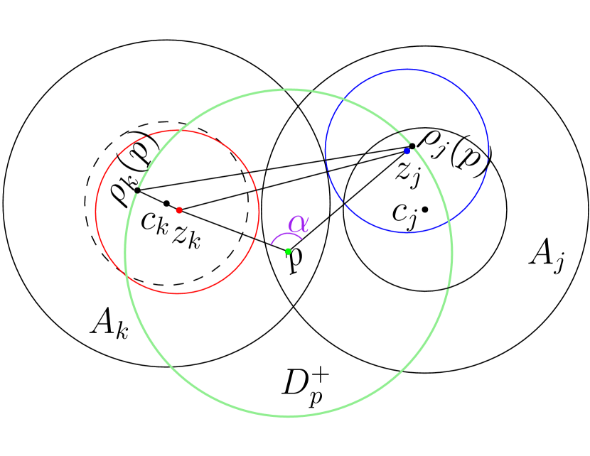
Let be an instance of MRMP-RA. Let be the number of robots and be the complexity of the environment . We describe an algorithm for computing a weakly-monotone path ensemble for such that . We remark that is weakly-monotone but need not be, i.e. is an -approximation of any feasible motion plan. We parameterize the paths in over the common interval . We need a few definitions and concepts related to revolving areas. For any , let denote the center of the revolving area , and let (resp. ) be the disc of radius (resp. 3) centered at , i.e., . If then . We refer to and as the core and buffer, respectively, of revolving area . See Figure 1.
Overview of the Algorithm.
The algorithm consists of three stages. We note that Stage (I) and (II) are used in [17]. However, Stage (III) differs significantly from previous work in order to ensure the total cost of paths is within an factor of that of the optimal motion plan. We describe all stages for completeness.
- I.
-
We compute the free space (with respect to one robot) using the algorithm of Ó’Dúnlaing and Yap [24, 13]. If and , for some , do not lie in the same connected component of , then a feasible path does not exist for from to . Therefore, we stop and return that no feasible motion plan exists from to . Next, for each , we compute a shortest path from to , ignoring other robots using the algorithm of Chen and Wang [5]. Let be the path ensemble computed by the algorithm.
Although does not intersect , it may not be feasible since two robots may collide during the motion. The next two steps deform to convert it into a feasible motion plan. We take an arbitrary permutation of . Without loss of generality assume . We say that is active during the subinterval of , during which it moves from to . During (resp. ) only moves within the revolving area (resp. ).
- II.
-
For each , we first modify , as described below in Section 3.1, so that it does not intersect the interior of the core of any revolving area that is occupied by a robot , for ; see Figure 3. Let be the deformed path. Abusing the notation a little, let denote a uniform parameterization of the path , i.e. moves with a fixed speed during from to along . We extend to the interval by setting for and for . Set .
- III.
-
Next, for each distinct pair , we construct a retraction map that specifies the position of for a given position of during the interval when is active so that and do not collide as moves along . The retraction map ensures that stays within the revolving area (resp. ) for (resp. ), and it does not collide with any for , as well. See Figure 3. Using this retraction map, we construct the path as follows:
We prove below that each is a continuous path. In Section 4, we prove that is a feasible path ensemble with .
3.1 Modifying path
Fix an . For , let and for , let . Set . This step modifies to ensure that the path of does not enter the core of any .
Fix a . If , then does not affect . If , then we modify as follows: let , be the first and last intersection points of and along , respectively. Let be the shorter arc of , the boundary of the core , between and . We replace with . We repeat this step for all . Let be the resulting path from to ; does not intersect for any . Note that ’s are pairwise disjoint, and that is a shortest path from to in , therefore and , for any pair , are disjoint. We can thus process in an arbitrary order and the resulting path does not depend on the ordering. Furthermore (since ), so for all .
3.2 Retracting a robot
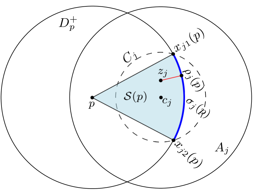
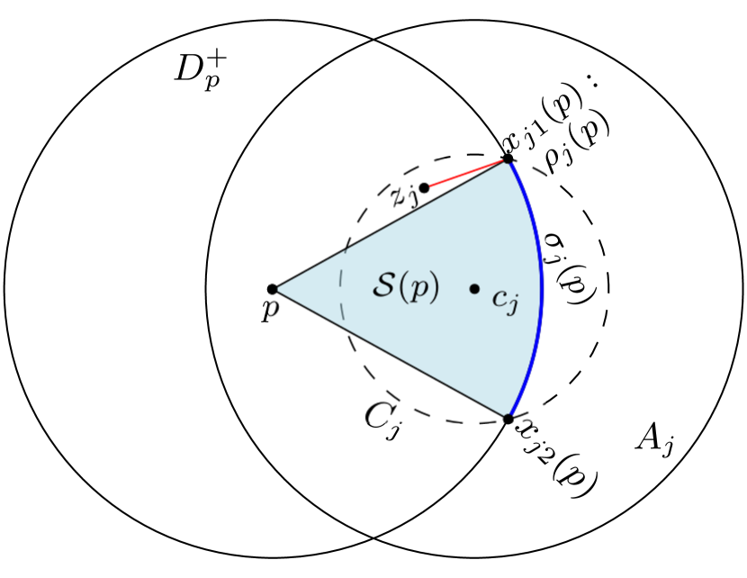
We now describe the retraction motion of when is active, so that they do not collide. Note that for all , , i.e., before applying the retraction is at when is active. We define the retraction function that specifies the motion of within during . Since is fixed, for simplicity we use to denote , and we use (resp. ) for disc (resp. ). If the center of is at distance at least from , then does not intersect , so there is no need to move from . Therefore we set for all such that . On the other hand, does not intersect the interior of so is undefined for . We thus focus on the case when , in which case lies in the buffer disc , and , i.e., .
Let be the disc of radius centered at . Note that for a point , if and only if . Intuitively, we move the center of from (within ) as little as possible so that does not collide with . Formally, we define as: if , and undefined otherwise.
In the remainder of the discussion, we assume and , so . Therefore, exists and additionally is unique. We now discuss the two possible types of retraction. Refer to Figure 4 throughout this paragraph. Note that and intersect at exactly two points since , say, . Let be the smaller of the two arcs of induced by and , and let be the sector of induced by , . Observe that the retraction point lies on . If , then is the intersection point of the ray with , as the closest point in from is on the straight line from to . Since lies inside , . If , the retraction point is , i.e., the closest point to in is an endpoint of . Note that our retraction ensures that will be centered back at after robot moves away.
In the remainder of the paper, if we say the that the retraction is of intersection type, otherwise we say that the retraction is of sector type. Since for all and none of the ’s enter , the retraction path of lies in . We conclude this section with the following lemma, which follows from the fact that is a continuous function, for all such that , and .
Lemma 6.
For any , is a continuous path from to .
4 Correctness and Analysis of the Algorithm
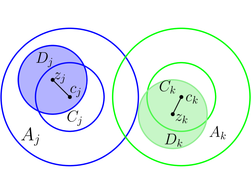
We first prove that is feasible (Section 4.1), then we bound (Section 4.2), and finally analyze the running time in Section 4.3. We begin by summarizing a few relevant properties of revolving areas (see Figure 5), which are straightforward to prove.
Lemma 7.
4.1 Feasibility
In this section, we show that path ensemble is feasible. Recall that stage (I) of the algorithm reports that there is no feasible solution if any and do not lie in the same connected component. So assume that Stage I computes a feasible path for each . Stages II and III modify these paths so that they remain in . Hence, we only need to show that no two robots collide with each other during the motion, i.e., for any and for any , . We fix some and the corresponding active interval and prove the feasibility of during this interval. Note that is the only active robot in and other robots stay in their revolving areas. By the definition of retraction, for any , and for any , , so does not collide with during interval . Thus, we only need to show that for any pair , and do not collide while moves along its retraction path. Since Lemma 9 holds for any interval , we obtain the final statement of feasibility.
Lemma 8.
For any and , the minimum distance between the line segments and is at least , i.e.,
Proof.
Let be the closest pair of points on the segments and . Note that and are disjoint since and and these cores do not intersect (cf Lemma 7). This implies that either or must be an endpoint of the respective segment. Assume without loss of generality that is an endpoint of . By Lemma 7, . Let be the endpoint of at distance from ( if and otherwise). Since , , Then . ∎
Lemma 9.
For any , and do not collide during the interval .
Proof.
In view of the above discussion, we assume . The claim is equivalent to showing that for every . Let . There are two cases:
Case 1: or .
Without loss of generality, assume that . By construction, , therefore by Lemma 7(iii), .
Case 2: and .
Recall is the disc of radius 2 centered at , and are the intersection points of the core of and . In this case, . We consider the triangle formed by the retraction points , and . We show that . We will first define a point based on the current retraction type of . If the retraction of is type sector, then lies within the sector , let . Otherwise, the retraction is of type intersection and without loss of generality we assume is . In this case, consider the segments and . These two segments must intersect, as and . We let be the intersection point of segments. Note that in either case, lies on segment . We analogously define . See Figure 6 for an example where and . By definition, and and Lemma 8 implies that . Additionally, , so (similarly ). Let be the angle . Since , and , . Now consider the triangle formed by the retraction points and . By construction, . The distance between and each retraction point is : . This implies the other two angles in the triangle are equal (). Since , is the longest edge of the triangle . The other two sides have length , so , as desired. ∎
Corollary 10.
The path ensemble returned by the algorithm is feasible.
4.2 Cost of path ensemble
We now analyze the cost of the path ensemble the algorithm returns. The algorithm starts by computing , the shortest paths of all robots in while ignoring other robots. Clearly, we have . We show that . Stage (II) of the algorithm deforms to . Path only if for some , otherwise . Suppose for some . Then in , is replaced with the shorter arc of , determined by the first and last endpoints, say and , of . Therefore, . Hence, and we obtain: .
We now focus on bounding the length of retraction paths of non-active robots, which is one of the main technical contributions of the paper. Let , and let , i.e., is the retraction of due to the motion of and is the part of that causes the retraction motion of . Refer to Figure 3. We show that (cf Corollary 16) and charge to . We bound by splitting into two scenarios. Roughly speaking, if does not penetrate the buffer too deeply, we use a Lipschitz condition on the retraction map to show . More concretely, for , let be the disk of radius centered at . We prove a Lipschitz condition when the active robot lies outside (cf Corollary 14). On the other hand, if travels into then the Lipschitz condition may not hold, but we argue that and that (cf Lemma 15). Finally, using a packing argument, we show that each “point" of is only charged times, and thus .
Cost of .
Stage (II) of the algorithm deforms to . Path only if for some , otherwise . Suppose for some . Then in , is replaced with the shorter arc of , determined by the first and last endpoints, say and , of . Therefore, . Hence, and we obtain:
Lemma 11.
.
Retraction of outside .
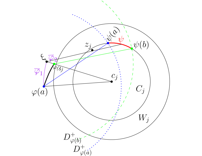
As in Section 4.1, we fix an interval for some . Let . That is, is the interval(s) of time in which the path of robot forces the retraction of robot while the center of lies outside . Let be the restriction of path of robot during the interval , i.e. for . Let be the retraction of during , i.e., for . We show that by proving a Lipschitz condition on .
We will divide into subpaths, referred to as pathlets, so that there is only one type of retraction point associated with the subpath. We call a time instance an event if is either an endpoint of a connected component of (i.e., or ) or , (i.e., the type of retraction point changes at time ). Let be the event points. We divide and into pathlets at these events, i.e., and where and . We prove the Lipschitz condition for each pathlet. All points on have the same type of of retraction by construction of . We call a sector-type (intersection-type) pathlet if all points have sector (resp. intersection) type retraction.

Lemma 12.
For a sector-type pathlet of , .
Proof.
For each , is type sector, i.e. lies on the ray at distance from . In this case, the retraction map traces a portion of a Conchoid [15].
We parameterize points on and using polar coordinates, with as the origin. Let be a point on , where is the orientation of the point with respect to the -axis (with as the origin). Then, . See Figure 7. Note that and . Since lies outside and , we have . Therefore, and . Hence,
Lemma 13.
For an intersection-type pathlet of , .
Proof.
Again, we prove the lemma by showing that a Lipschitz condition holds. Let . We parameterize both and in polar coordinates, but with as the origin. Let be the interval over which is defined. Let for . We assume that is sufficiently small (otherwise we divide it into smaller pathlets and argue for each pathlet) so that both - and -monotone.
Set and . Since lies outside , for all . W.l.o.g., assume both and are monotonically non-decreasing. We obtain:
The retraction path varies monotonically on the unit circle . Thus, we parameterize by its direction on , and . To bound , consider the following path from to , see Figure 7. Let be the arc from to point along the circle of radius centered at . Let be the segment to , this is a radial segment on line . Then, . Since the radius along does not change, .
For a point , the orientation of is (by the law of cosines, considering triangle ). Since does not change along and , we obtain .
Putting everything together, ∎
Corollary 14.
Let . Let be the portion of during the interval such that and , and let be the retraction of corresponding to . Then .
Retraction path inside .
Recall that does not intersect , but possibly travels along . For a point , if , then is the point on diametrically opposite . Thus, . In the following, we consider only .
Lemma 15.
For a pathlet (i.e., a connected subpath) of path such that for some , .
Proof.
Since , , therefore we only need to argue that is constant. We will bound the length of both types of retraction maps (intersection and sector) separately for , and use the sum as an upper bound on the length of the actual retraction map.
Sector retraction. We consider the sector type retraction map. Let be the origin and consider polar coordinates. Let be the sector type retraction point with respect to . Since is a subpath of a shortest path in , we can divide into at most two pathlets such that each piece is -monotone. Abusing notation, let be one of these pieces with endpoints and .
We write the retraction point parameterized by as . Using the fact that for all , the arc length of the retraction map is
Therefore, , for each .
Intersection retraction. We consider the retraction map defined by an intersection point of and . We now let be the origin and consider polar coordinates. Let be the intersection type retraction point closest to with respect to . Again, we divide into at most two pathlets such that each of them is -monotone (one pathlet is the portion of coming closer to the core , and the other moves away from ). Let be one of the pathlets with endpoints and . The retraction point lies on the unit circle , and as changes monotonically from to , the retraction point moves monotonically on . Therefore, .
Finally, , as claimed. ∎
Applying Lemma 15 to each of (at most two) connected components of and combining with Corollary 14, we obtain the following:
Corollary 16.
For , let be defined as and let . Then .
Cost of Path Ensemble.
We are now ready to bound the cost of the path ensemble returned by the algorithm.
Lemma 17.
For an instance of optimal MRMP with revolving areas, let be the path ensemble returned by the algorithm. Then .
Proof.
Set . We already argued that , where is the path ensemble computed in stage II of the algorithm. We thus need to prove . For a pair , let . By construction, . For a fixed ,
Where the last equality follows from Corollary 16. Hence,
By definition of , and . Fix a point . Consider a disk of radius centered at . If for some , then . Since cores are pairwise-disjoint (cf Lemma 7(i)), can contain at most core disks and any lies in ’s. Therefore,
Plugging this back in we obtain: ∎
4.3 Running-time Analysis
The algorithm has three stages. In the first stage, we compute the free space with respect to one robot, which takes time, by computing the Voronoi of , see the algorithm of [24], and see [3] for details. In the same stage, we compute a set of shortest paths for discs, using the algorithm of [5], taking time in total over all robots. Each path has complexity . In stage two of the algorithm, is modified to avoid the core of any occupied revolving area, increasing the complexity of each curve to . In stage three of the algorithm, the deformed paths are again edited to include retraction maps in which non-active robots may move within their revolving area. It suffices to bound the number of breakpoints in the final path that correspond to retracted maps. Let be such a breakpoint on , which is for some . There are two cases: (i) the preimage of on is a breakpoint of , or (ii) (i.e., forces to move within the revolving area). We charge both of these breakpoints to . Since the preimage of lies in the buffer disk of , using a packing argument similar to the proof of Lemma 17 below, we can show that breakpoints are charged to .
Theorem 18.
Let be an instance of optimal MRMP with revolving areas, and let be the complexity of . If a feasible motion plan of exists then a path ensemble of cost can be computed in time.
We conclude this section by noting that since the ordering (of active robots) is arbitrary, the algorithm can be extended to an online setting where and are given in an online manner (as long as each given satisfies the revolving area property). Our algorithm is -competitive for this setting, i.e., the cost is times the optimal cost of the offline problem.
5 Computing a Good Ordering
In the previous section, we proved that the total cost of the path ensemble is irrespective of the order in which the robots moved. However, the order in which robots move has a significant impact on how the paths are edited in Stages (II) and (III). The increase in cost because of editing may vary between and depending on the ordering (see [17] for a related argument). For a path ensemble computed by our algorithm, let , which we refer to as the marginal cost of , where is the path ensemble computed in Stage (I). For a permutation of , let be the path ensemble computed by the algorithm if robots were moved in the order determined by . Set . Finally, set where the minimum is taken over all permutations of .
Adapting the construction in [17], we can show that the problem of determining whether , for some , is NP-hard. We present an approximation algorithm for computing a good ordering such that .
Our main observation is that , the marginal cost of an ordering , is decomposable, in the sense made precise below. For a pair , we define to be the contribution of the pair to the marginal cost of an ordering , assuming , i.e., how much the shortest path has to be modified because of and vice-versa assuming is active before . Note that if then (resp. ) is at (resp ) when (resp is active. There are two components of : (i) (resp. ) enters the core (resp. ) in (resp. ), (ii) retraction motion of (resp. ) when (resp. ) enters the buffer disc (resp. ).
Let (resp. ) be the arc of (resp. ) with which (resp. ) is replaced with. Then is the contribution of (i) to . For (ii), we define (resp. ) be the retraction map of because of when is active before (resp. after) . Then From the previous two components, we have
We now reduce the problem of computing an optimal ordering to instance of weighted feedback-arc-set (FAS) problem. Given a directed graph with weights on the edges, , a feedback arc set is a subset of edges of whose removal makes a directed acyclic graph. The weight of , is . The FAS problem asks to compute an FAS of the smallest weight. It is known to be NP-complete.
Given an MRMP-RA instance , we first compute as in stage (I) of the algorithm. Next, for each pair , we construct a directed graph as follows. is a complete directed graph with , one representing each robot, , . It can be shown that each feedback arc set of induces an ordering on , and vice versa. Furthermore, . Even et al. [8] have described a polynomial-time -approximation algorithm for the FAS problem. By applying their algorithm to , we obtain the following.
Theorem 19.
Let be an instance of optimal MMP with revolving areas, and let be the complexity of . Let the optimal order of execution of paths be . An ordering with can be computed in polynomial time in and .
6 Conclusion
In this work, we presented the first constant-factor approximation algorithm for computing a feasible weakly-monotone motion plan to minimize the sum of distances traveled. Additionally, the algorithm can be extended to an online setting where the polygonal environment is fixed, but the initial and final positions of the robots are specified in an online manner. On the hardness side, we prove that minimizing the total traveled distance, even with the restriction of a weakly-monotone motion plan, is APX-hard.
There are several interesting open questions. The first is whether the constant factor approximation presented in this work can be improved; another is whether there are instances in which the separation bounds for revolving areas are not required or can be tightened. There are other objectives to consider; instead of the sum of distances objective, one can consider the makespan (latest arrival time), where little is known even for a small number of discs in the presence of obstacles.
References
- [1] Aviv Adler, Mark de Berg, Dan Halperin, and Kiril Solovey. Efficient multi-robot motion planning for unlabeled discs in simple polygons. IEEE Trans Autom. Sci. Eng., 12(4):1309–1317, 2015.
- [2] Bahareh Banyassady, Mark de Berg, Karl Bringmann, Kevin Buchin, Henning Fernau, Dan Halperin, Irina Kostitsyna, Yoshio Okamoto, and Stijn Slot. Unlabeled Multi-Robot Motion Planning with Tighter Separation Bounds. In 38th International Symposium on Computational Geometry (SoCG), 2022.
- [3] Eric Berberich, Dan Halperin, Michael Kerber, and Roza Pogalnikova. Deconstructing approximate offsets. Discret. Comput. Geom., 48(4):964–989, 2012.
- [4] Josh Brunner, Lily Chung, Erik D. Demaine, Dylan H. Hendrickson, Adam Hesterberg, Adam Suhl, and Avi Zeff. 1 X 1 rush hour with fixed blocks is PSPACE-complete. In 10th International Conference on Fun with Algorithms, volume 157, pages 7:1–7:14, 2021.
- [5] Danny Z Chen and Haitao Wang. Computing shortest paths among curved obstacles in the plane. ACM Transactions on Algorithms, 11(4):1–46, 2015.
- [6] Dror Dayan, Kiril Solovey, Marco Pavone, and Dan Halperin. Near-optimal multi-robot motion planning with finite sampling. In IEEE International Conference on Robotics and Automation, pages 9190–9196, 2021.
- [7] Erik D. Demaine, Sándor P. Fekete, Phillip Keldenich, Henk Meijer, and Christian Scheffer. Coordinated motion planning: Reconfiguring a swarm of labeled robots with bounded stretch. SIAM Journal on Computing, 48(6):1727–1762, 2019.
- [8] Guy Even, J Seffi Naor, Baruch Schieber, and Madhu Sudan. Approximating minimum feedback sets and multicuts in directed graphs. Algorithmica, 20(2):151–174, 1998.
- [9] Tzvika Geft and Dan Halperin. Tractability frontiers in multi-robot coordination and geometric reconfiguration, 2021. arXiv:2104.07011.
- [10] Tzvika Geft and Dan Halperin. Refined hardness of distance-optimal multi-agent path finding. In 21st International Conference on Autonomous Agents and Multiagent Systems, AAMAS, pages 481–488, 2022.
- [11] John E Hopcroft, Jacob Theodore Schwartz, and Micha Sharir. On the complexity of motion planning for multiple independent objects; PSPACE-hardness of the "warehouseman’s problem". The International Journal of Robotics Research, 3(4):76–88, 1984.
- [12] Sertac Karaman and Emilio Frazzoli. Sampling-based algorithms for optimal motion planning. International Journal of Robotics Research, 30(7):846–894, 2011.
- [13] C O’Ddnlaing and CK Yap. A retraction method for planning the motion of a disc. J. Algorithms, 6:104–111, 1985.
- [14] Oren Salzman. Sampling-based robot motion planning. Commun. ACM, 62(10):54–63, 2019.
- [15] Jacob T Schwartz and Micha Sharir. On the piano movers’ problem: III. coordinating the motion of several independent bodies: The special case of circular bodies moving amidst polygonal barriers. The International Journal of Robotics Research, 2(3):46–75, 1983.
- [16] Rahul Shome, Kiril Solovey, Andrew Dobson, Dan Halperin, and Kostas E. Bekris. dRRT: Scalable and informed asymptotically-optimal multi-robot motion planning. Auton. Robots, 44(3-4):443–467, 2020.
- [17] Israela Solomon and Dan Halperin. Motion planning for multiple unit-ball robots in . In Workshop on the Algorithmic Foundations of Robotics, WAFR, pages 799–816, 2018.
- [18] Kiril Solovey and Dan Halperin. On the hardness of unlabeled multi-robot motion planning. Int. J. Robotics Res., 35(14):1750–1759, 2016.
- [19] Kiril Solovey, Lucas Janson, Edward Schmerling, Emilio Frazzoli, and Marco Pavone. Revisiting the asymptotic optimality of RRT. In 2020 IEEE International Conference on Robotics and Automation, ICRA 2020, Paris, France, May 31 - August 31, 2020, pages 2189–2195. IEEE, 2020.
- [20] Kiril Solovey, Jingjin Yu, Or Zamir, and Dan Halperin. Motion planning for unlabeled discs with optimality guarantees. In Robotics: Science and Systems, 2015.
- [21] Roni Stern, Nathan R. Sturtevant, Ariel Felner, Sven Koenig, Hang Ma, Thayne T. Walker, Jiaoyang Li, Dor Atzmon, Liron Cohen, T. K. Satish Kumar, Roman Barták, and Eli Boyarski. Multi-agent pathfinding: Definitions, variants, and benchmarks. In Proc. 12th International Symposium on Combinatorial Search, pages 151–159, 2019.
- [22] Matthew Turpin, Kartik Mohta, Nathan Michael, and Vijay Kumar. Goal assignment and trajectory planning for large teams of interchangeable robots. Auton. Robots, 37(4):401–415, 2014.
- [23] Vijay V Vazirani. Approximation algorithms. Springer, 2001.
- [24] Chee-Keng Yap. An O (n log n) algorithm for the voronoi diagram of a set of simple curve segments. Discret. Comput. Geom., 2:365–393, 1987.