HIGH-ENERGY PHOTON OPACITY IN THE
TWISTED MAGNETOSPHERES OF MAGNETARS

Abstract

Magnetars are neutron stars characterized by strong surface magnetic fields generally exceeding the quantum critical value of 44.1 TeraGauss. High-energy photons propagating in their magnetospheres can be attenuated by QED processes like photon splitting and magnetic pair creation. In this paper, we compute the opacities due to photon splitting and pair creation by photons emitted anywhere in the magnetosphere of a magnetar. Axisymmetric, twisted dipole field configurations embedded in the Schwarzschild metric are treated. The paper computes the maximum energies for photon transparency that permit propagation to infinity in curved spacetime. Special emphasis is given to cases where photons are generated along magnetic field loops and/or in polar regions; these cases directly relate to resonant inverse Compton scattering models for the hard X-ray emission from magnetars and Comptonized soft gamma-ray emission from giant flares. We find that increases in magnetospheric twists raise or lower photon opacities, depending on both the emission locale, and the competition between field line straightening and field strength enhancement. Consequently, given the implicit spectral transparency of hard X-ray bursts and persistent “tail” emission of magnetars, photon splitting considerations constrain their emission region locales and the twist angle of the magnetosphere; these constraints can be probed by future soft gamma-ray telescopes such as COSI and AMEGO. The inclusion of twists generally increases the opaque volume of pair creation by photons above its threshold, except when photons are emitted in polar regions and approximately parallel to the field.

1 Introduction

Magnetars are highly-magnetized neutron stars with periods $\,P\,$ generally in the 2–12 sec range. They exhibit persistent X-ray emission in the $\,<10\,$keV band, with both thermal and non-thermal components (e.g., see Viganò, 2013), with luminosities $\,L_{X}\sim 10^{33}-10^{35}\,$erg/sec that exceed the electromagnetic torque spin-down values $\,L_{\rm sd}\propto{\dot{P}}/P^{3}\,$ inferred from observed values of $\,P\,$ and $\,\dot{P}\,$. About a third of the population also exhibits persistent, hard non-thermal emission in the 10-300 keV band. This timing information is employed to discern that their surface magnetic fields mostly exceed the quantum critical value of $\,B_{\rm cr}=m_{e}^{2}c^{3}/(e\hbar)\approx 4.41\times 10^{13}\,$Gauss, where the electron cyclotron and rest mass energies are equal. Such superstrong fields are a distinguishing hallmark of magnetars: they are believed to power their sporadic X-ray burst emission (Duncan & Thompson, 1992; Thompson & Duncan, 1996). Most of this transient activity consists of short hard X-ray flares of subsecond duration with luminosities in the $\,10^{38}\,$erg/sec $\,<L_{X}<10^{42}\,$ erg/sec range. The trapping of magnetospheric plasma for such durations requires the presence of strong magnetic fields. For recent magnetar reviews, see Turolla et al. (2015) and Kaspi & Beloborodov (2017). The observational status quo of magnetars is also summarized in the McGill Magnetar Catalog (Olausen & Kaspi, 2014) and its online portal.

While the thermal signals from magnetars below around 5 keV provide key information for understanding their surfaces, it is the magnetospheric signals above 10 keV that are germane to the study here. There are three types of hard X-ray/soft gamma-ray emission exhibited by magnetars. The first of these consists of steady, hard, non-thermal pulsed spectral tails that have been detected in around ten magnetars (Kuiper et al., 2006; Götz et al., 2006; den Hartog et al., 2008a, b; Enoto et al., 2010; Younes et al., 2017). These luminous tails, usually fit with power-law spectral models of $\,F_{\nu}\,$ index between 0 and 1, extend up to 150 - 250 keV, with a turnover around 500 - 750 keV implied by constraining pre-2000 COMPTEL upper limits. The Fermi-Gamma-Ray Burst Monitor (GBM) has also observed these tails (ter Beek, 2012), providing the sensitivity to better measure the flux above 100 keV. Over the last decade, much more Fermi-GBM data on magnetars has been accumulated, enabling improved spectral definition, yet with no material change in the overall shape of the tails (Kuiper, private comm.). The Fermi-Large Area Telescope (LAT) has not detected this component (e.g., Abdo et al., 2010; Li et al., 2017). The most prominent model for the generation of these tails is inverse Compton scattering, resonant at the cyclotron frequency in the strong magnetar fields: see Baring & Harding (2007); Fernández & Thompson (2007); Beloborodov (2013); Wadiasingh et al. (2018).

Transient, recurrent bursts are observed for many magnetars, both for the soft gamma repeater (SGR) and anomalous X-ray pulsar (AXP) varieties. Some episodes of such bursts last hours to days, over which tens to hundreds of individual short bursts can occur. Given their typical $\,\sim 0.01-0.3\,$sec durations and super-Eddington luminosities, they must be generated from highly optically thick magnetospheric regions. The bursts mostly have emission below around 100 keV, with a spectral breadth (Göǧüş et al., 1999; Feroci et al., 2004; Israel et al., 2008; Lin et al., 2012; van der Horst et al., 2012; Younes et al., 2014) that indicates thermal gradients and strong Comptonization (Lin et al., 2011) in the emission regions. For occasional exceptional bursts, the observed maximum observed energy is somewhat higher, for example, two anomalously hard bursts from SGR 1900+14 (Woods et al., 1999) observed in late 1998 and early 1999. A more recent notable exemplar is the steeper spectrum FRB-X burst (Mereghetti et al., 2020; Li et al., 2021; Ridnaia et al., 2021) associated with the fast radio burst (FRB) seen in April 2020 from SGR 1935+2154, being spectrally unique among the population of bursts detected from this magnetar Younes et al. (2021).

There are also the rare giant flares from magnetars, highly optically thick to Compton scattering and with luminosities $\,10^{44}-10^{47}\,$ erg/sec at hard X-ray energies extending up to around 1 MeV. They have been observed for only two SGRs in the Milky Way (e.g., Hurley et al., 1999b, 2005) and one in the Large Magellanic Cloud (e.g., Mazets et al., 1979). They are characterized by a short, intense spike of duration $\,\sim 0.2\,$s, followed by a pulsating tail lasting several minutes that is spectrally softer. In April 2020, a giant flare was detected from a magnetar in the galaxy NGC 253 at 3.5 Mpc distance, exhibiting only the initial spike in Fermi-GBM observations up to around 3 MeV (Roberts et al., 2021), followed by delayed GeV emission seen by Fermi-LAT (Ajello et al., 2021). This event provided the clearest view to date of the MeV-band spectral evolution of giant flares.

Key questions surrounding these three varieties of magnetar hard X-ray signals are: where in the magnetosphere do they originate, how does the magnetic field modulate and power their activity, and what physics controls their spectral character? A central element concerns how prolifically electron-positron pairs are created. This paper focuses on two exotic QED processes operating in magnetar magnetospheres, magnetic pair creation $\,\gamma\to e^{\pm}\,$, permitted above its threshold energy of $\,2m_{e}c^{2}\,$, and magnetic photon splitting $\,\gamma\to\gamma\gamma\,$, which can attenuate photons all the way down to around 50 keV in magnetar fields (Baring & Harding, 2001). These processes are permitted only in the presence of magnetic fields (e.g., Erber, 1966; Adler, 1971), and both possess rates that are extremely sensitive to the strength of the magnetic field B, the angle $\,\Theta_{\hbox{\sixrm kB}}\,$ that photons propagate relative to the field direction, and the energy of a photon. Many of their pertinent properties including magnetospheric opacity have been addressed in numerous papers (Baring, 1995; Harding, Baring & Gonthier, 1997; Baring & Harding, 1998, 2001; Story & Baring, 2014). In particular, the suppression of pair creation by photon splitting in neutron star magnetospheres was discussed by Baring & Harding (1998) as a possible means for generating a “radio death line” for high-field pulsars.

Recently, Hu et al. (2019) calculated photon splitting and pair creation opacities in the inner magnetospheres of high B neutron stars, applicable to arbitrary colatitudes and a substantial range of altitudes in closed field line zones. This work determined both attenuation lengths and escape energies for each process, the latter being the maximum photon energy for which the magnetosphere is transparent. Yet it restricted its focus to general relativistic dipole field geometries.

A major element of the magnetar paradigm is the force-free MHD distortion of field line morphology incurred by large pair currents (e.g., Thompson, Lyutikov & Kulkarni, 2002; Beloborodov, 2013; Chen & Beloborodov, 2017). In this scenario, magnetic and other stresses in the crust are released via surface shear motions that rotate the external field lines within flux tubes/surfaces, thereby generating magnetospheric helicity. The twisted configuration can be sustained for extended time periods by magnetospheric currents due to $\,e^{-}-e^{+}\,$ pairs created in electrostatic potential gaps, likely somewhat near polar zones. The twists require both toroidal and poloidal currents (e.g., Thompson, Lyutikov & Kulkarni, 2002; Beloborodov, 2009): toroidal currents straighten the poloidal magnetic field lines, and poloidal currents support the toroidal field components. These twisted fields, superposed on the global quasi-dipolar magnetic structure, serve as energy reservoirs and thus couple intimately to magnetospheric activation. Twists thus increase the local magnetic field strength $\,B\,$, change the radii of field curvature, two influences that profoundly alter photon splitting and pair opacity in magnetars, raising and (sometimes) lowering the escape energy. Here we extend the analysis of Hu et al. (2019) to address twisted field morphologies, embedding the ideal MHD flat spacetime prescription in the Schwarzschild metric.

This construction is detailed in Section 3, following a summary of the opacity geometry and the QED physics of magnetic photon splitting and pair creation in Section 2. Results are presented in Sections 4 and 5.1. The introduction of twisted fields to the magnetosphere increases the volumes of opaque regions spanning mid-latitudes to the magnetic equator, since the twist changes the field morphology and increases the field magnitude. For photons emitted from specific field loops, twisted magnetospheres establish higher photon escape energies because of the straightening of the field lines and the accompanying rise of the emission altitudes. The effectiveness of photon splitting as a competitor to pair creation increases near the polar regions as the cumulative azimuthal shear angle $\,\Delta\phi_{\rm tw}\,$ of the magnetic twist increases. Contextual discussion of the results is presented in Sec. 5.2.

2 Opacity Geometry and Physics

This section summarizes the set-up for our radiative transfer opacity calculations, namely the geometry and the QED physics pertinent to the attenuation.

2.1 Radiative Transfer Geometry

The optical depth for a photon emitted at any locale $\,\bm{r}_{\hbox{\fiverm E}}\,$ in the magnetosphere (in the observer’s coordinate frame; OF) in direction $\,\hat{\bm{k}}_{\hbox{\fiverm E}}\,$ is given by

$$\tau(l)\;=\;\int_{0}^{l}{\cal{R}}\bigl{(}\varepsilon_{\infty},\hat{\bm{k}}_{\hbox{\fiverm E}},\bm{r}_{\hbox{\fiverm E}};\Theta_{\hbox{\sixrm kB}},\bm{B}\bigr{)}\,ds\quad,$$ (1)

where $\,\cal{R}\,$ is the attenuation coefficient (in units of cm^-1) and $\,l\,$ is the cumulative proper length of the photon trajectory. Here $\,\varepsilon_{\infty}m_{e}c^{2}\,$ is the observed photon energy at infinity. In considering general relativistic photon propagation, the optical depth is integrated over the geodesic path-length $\,s\,$, sampling different local inertial frames (LIFs) with altitude. Thus $\,\bm{B}\equiv\bm{B}_{\rm GR}\,$ is the LIF frame magnetic field, specified in Eq. (15) below, and $\,\Theta_{\hbox{\sixrm kB}}\,$ is the angle between the field and the photon momentum in the LIF, which satisfies Eq. (3). The attenuation length $\,L\,$ is defined (Baring & Harding, 2001; Story & Baring, 2014; Hu et al., 2019) to be the proper distance over which optical depth $\,\tau(L)=1\,$. The principal quantity of interest in our opacity considerations is the escape energy $\,\varepsilon_{\rm esc}\,$, which is defined as the OF photon energy at which the attenuation length $\,L\,$ becomes infinite:

$$1\;=\;\int_{0}^{\infty}{\cal{R}}\bigl{(}\varepsilon_{\rm esc},\hat{\bm{k}}_{\hbox{\fiverm E}},\bm{r}_{\hbox{\fiverm E}};\Theta_{\hbox{\sixrm kB}},\bm{B}\bigr{)}\,ds\quad.$$ (2)

Since the attenuation coefficients increase rapidly with photon energy for both photon splitting and pair creation, the optical depth satisfies $\,\tau<1\,$ for photons with energies $\,\varepsilon\,$ smaller than the escape energy $\,\varepsilon_{\rm esc}\,$. Thus the escape energy $\,\varepsilon_{\rm esc}\,$ represents the photon energy below which the magnetosphere is transparent. It is a strong function of the emission locale (at which $\,s=0\,$) and the magnetic field morphology, features that are central to the considerations of the paper.

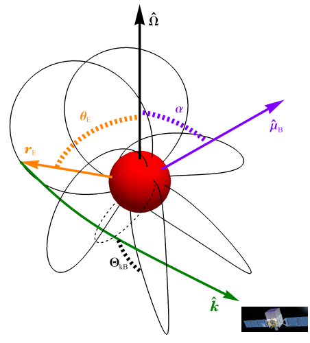
Figure 1: Schematic diagram displaying the photon propagation geometry in a twisted magnetosphere. The rotation axis $\,\hat{\bm{\Omega}}\,$ is depicted as black arrow, and the magnetic dipole moment vector $\,\hat{\bm{\mu}}_{\hbox{\sixrm B}}\,$ at one particular rotational phase is displayed as the purple arrow. The star’s magnetic inclination is $\,\alpha=\arccos[\hat{\bm{\mu}}_{\hbox{\sixrm B}}\cdot\hat{\bm{\Omega}}]\,$. One photon is emitted at $\,\bm{r}_{\hbox{\fiverm E}}\,$ (emission polar angle $\,\theta_{\hbox{\fiverm E}}=\arccos[\hat{\bm{r}}_{\hbox{\fiverm E}}\cdot\hat{\bm{\Omega}}]\,$) and propagates through the foreground of the magnetosphere: the trajectory of the photon is represented by a green curve, lying in front of the star; $\,\hat{\bm{k}}\,$ signifies the changing direction (unit momentum vector) of the photon. Twisted field loops with a $\,p=0.75\,$ ($\Delta\Phi_{\rm tw}=84^{\circ}$) parameterization in the Schwarzschild metric ($\,M_{\hbox{\sixrm NS}}=1.44M_{\odot}\,$) are plotted as black curves anchored at a colatitude of $\,30^{\circ}\,$ relative to the magnetic axis. An untwisted field loop anchored at the same magnetic colatitude is also depicted as a dashed black curve for comparison. A representative angle $\,\Theta_{\hbox{\sixrm kB}}\,$ between the photon trajectory and a local magnetic field is highlighted.

The geometry of the attenuation process in the twisted magnetosphere of a rotating neutron star is depicted in Fig. 1, with the Fermi Gamma-Ray Space Telescope image being from its mission web page. The inclination angle between the stellar rotation axis and the magnetic axis is denoted as $\,\alpha\,$, and the colatitude of the emission locale relative to the rotation axis is denoted as $\,\theta_{\hbox{\fiverm E}}\,$. We consider photon propagation in the curved spacetime described by the Schwarzschild metric, fixing the stellar radius at $\,R_{\hbox{\sixrm NS}}=10^{6}\,$ cm and stellar mass at $\,M_{\hbox{\sixrm NS}}=1.44M_{\odot}\,$ throughout. For the schematic in Fig. 1, the photon path starts with emission parallel to $\,\bm{B}\,$, the focal case of Section 4.1. The optical depth in Eq. (1) is then integrated numerically over the geodesic path-length $\,s\,$, and at each point along the path, $\,{\cal R}\,$ is specified in the LIF. The trajectories of photons are integrated numerically in our calculation. These protocols are detailed in Section 5.1 of Hu et al. (2019). The opacity is very sensitive to the angle between the external magnetic field and the momentum vector of the propagating photon, which is given by

$$\cos\Theta_{\hbox{\sixrm kB}}\;=\;\hbox{${{\displaystyle\hat{\bm{k}}\cdot\bm{B}\vphantom{(}}\over{\displaystyle|\bm{B}|\vphantom{(}}}$}\quad\hbox{or}\quad\sin\Theta_{\hbox{\sixrm kB}}\;=\;\hbox{${{\displaystyle|\hat{\bm{k}}\times\bm{B}|\vphantom{(}}\over{\displaystyle|\bm{B}|\vphantom{(}}}$}\quad.$$ (3)

Although our formalism and associated computations are presented in curved spacetime, flat spacetime results can be easily obtained by specializing to $\,M_{\hbox{\sixrm NS}}\rightarrow 0\,$, and are used as a check of the results (see below).

In all results in this paper, the modulation of viewing geometry with stellar rotation phase will not be considered, as it was in Section 4.3 of Hu et al. (2019), where the pertinent behavior was detailed sufficiently. The primary interest here is in how twisted field morphology influences escape energies and the volume of magnetospheric opacity. Accordingly, it suffices to consider aligned rotators with $\,\alpha=0\,$ in the ensuing exposition, so that $\,\theta_{\hbox{\fiverm E}}\,$ represents the magnetic colatitude of emission at position vector $\,\bm{r}_{\hbox{\fiverm E}}\,$.

2.2 Photon Splitting and Pair Creation

The attenuation of photons is calculated for two linear polarization modes, namely $\,\parallel\,$ (ordinary) mode and $\,\perp\,$ (extraordinary) mode. Here $\,\perp\,$ and $\,\parallel\,$ refer to the states where photon electric vector is locally perpendicular and parallel to the plane containing the photon momentum vector $\,\bm{k}\,$ and the external field $\,\bm{B}\,$, respectively. These two linear modes approximately represent the polarization eigenmodes of soft X rays when vacuum polarization dominates the dielectric tensor of the magnetosphere of a magnetar. As the photon propagates in the magnetosphere, its electric field vector evolves adiabatically following the change of the magnetic field direction, with the birefringent QED vacuum ensuring that the polarization state (i.e., $\,\perp\,$ or $\,\parallel\,$) remains unchanged during propagation (see Heyl & Shaviv, 2000). This adiabatic polarization evolution persists out to the polarization-limiting radius, which is mostly beyond the escape altitudes for X-rays and gamma-rays that are highlighted in the various figures below. This feature simplifies the polarization transport considerably.

The opacity is computed for the two key processes that can be prolific in strong-field QED, namely photon splitting and pair creation. Here we provide a summary of the essentials of the rates for these processes, and detailed discussions of the physics for them can be found in Harding, Baring & Gonthier (1997), Baring & Harding (2001) and also in Harding & Lai (2006).

Magnetic photon splitting is a third-order QED process in which a single photon splits into two lower-energy photons. The CP invariance of QED permits only three splitting channels, namely: $\,\perp\rightarrow\parallel\parallel\,$, $\,\parallel\rightarrow\perp\parallel\,$ and $\,\perp\rightarrow\perp\perp\,$ (see Adler, 1971). In the domain of weak vacuum dispersion, $\,\perp\rightarrow\parallel\parallel\,$ is the only CP-permitted channel that satisfies energy-momentum conservation (Adler, 1971). This kinematic selection rule may not hold when plasma dispersion competes with the vacuum contribution in lower fields at higher altitudes where the cyclotron resonance can become influential. Thus, in the following presentation, we will consider all the CP-permitted splitting channels, and focus especially on polarization-averaged results, which differ only modestly from results where only $\,\perp\rightarrow\parallel\parallel\,$ is activated.

In the low-energy limit well below the pair creation threshold, applying to hard X-rays that are of principal interest here, the reaction rates for all the CP-permitted modes can be expressed as (Baring & Harding, 2001)

$${\cal R}^{\rm sp}_{\perp\to\parallel\parallel} = \hbox{${{\displaystyle\alpha_{\hbox{\sevenrm f}}^{3}\vphantom{(}}\over{\displaystyle 60\pi^{2}\lambda\hbox to0.0pt{\hss--}_{c}\vphantom{(}}}$}\,\varepsilon^{5}\,B^{6}\,{\cal M}_{1}^{2}\,\sin^{6}\Theta_{\hbox{\sixrm kB}}\;=\;\hbox{${{\displaystyle 1\vphantom{(}}\over{\displaystyle 2\vphantom{(}}}$}\,{\cal R}^{\rm sp}_{\parallel\to\perp\parallel}\quad,$$

$${\cal R}^{\rm sp}_{\perp\to\perp\perp} = \hbox{${{\displaystyle\alpha_{\hbox{\sevenrm f}}^{3}\vphantom{(}}\over{\displaystyle 60\pi^{2}\lambda\hbox to0.0pt{\hss--}_{c}\vphantom{(}}}$}\,\varepsilon^{5}\,B^{6}\,{\cal M}_{2}^{2}\,\sin^{6}\Theta_{\hbox{\sixrm kB}}\quad.$$

Here $\,\alpha_{\hbox{\sevenrm f}}\,$ is the fine structure constant, $\,\lambda\hbox to0.0pt{\hss--}_{c}\,$ is the reduced Compton wavelength of electron, and the field strength $\,B\,$ is expressed in the unit of the quantum critical field $\,B_{\rm cr}\,$. The LIF photon energy $\,\varepsilon\,$ is scaled by the rest mass energy of electron. For unpolarized photons, the attenuation coefficient can be obtained averaging Eq. (LABEL:eq:splitt_atten):

$${\cal R}^{\rm sp}_{\rm ave}\;=\;\hbox{${{\displaystyle\alpha_{\hbox{\sevenrm f}}^{3}\vphantom{(}}\over{\displaystyle 120\pi^{2}\lambda\hbox to0.0pt{\hss--}_{c}\vphantom{(}}}$}\,\varepsilon^{5}\,B^{6}\,\Bigl{(}3{\cal M}^{2}_{1}+{\cal M}^{2}_{2}\Bigr{)}\,\sin^{6}\Theta_{\hbox{\sixrm kB}}\quad,$$ (5)

a result detailed in Hu et al. (2019). The reaction rate coefficients $\,{\cal M}_{1},{\cal M}_{2}\,$ derived from squares of the matrix elements, are purely functions of $\,B\,$ in this low energy $\,\varepsilon\ll 1\,$ domain, possessing the forms

$${\cal M}_{\sigma}\;=\;\hbox{${{\displaystyle 1\vphantom{(}}\over{\displaystyle B^{4}\vphantom{(}}}$}\int_{0}^{\infty}\hbox{${{\displaystyle ds\vphantom{(}}\over{\displaystyle s\vphantom{(}}}$}e^{-s/B}\,\Lambda_{\sigma}(s)\quad,$$ (6)

with

$$\Lambda_{1}(s) = \left(-\frac{3}{4s}+\frac{s}{6}\right)\frac{\cosh s}{\sinh s}+\frac{3+2s^{2}}{12\sinh^{2}s}+\frac{s\cosh s}{2\sinh^{3}s}\quad,$$

$$\Lambda_{2}(s) = \frac{3}{4s}\frac{\cosh s}{\sinh s}+\frac{3-4s^{2}}{4\sinh^{2}s}-\frac{3s^{2}}{2\sinh^{4}s}\quad.$$

For low fields $\,B\ll 1\,$, $\,{\cal M}_{1}\approx 26/315\,$ and $\,{\cal M}_{2}\approx 48/315\,$ are independent of $\,B\,$, but at highly supercritical fields $\,B\gg 1\,$ possess $\,{\cal M}_{1}\propto B^{-3}\,$ and $\,{\cal M}_{2}\propto B^{-4}\,$ dependences.

One-photon pair creation is a first-order QED process that is allowed in the presence of a strong external field because momentum conservation orthogonal to B is then not operable. This conversion process is extremely efficient when $\,B\mathrel{\mathchoice{\lower 2.0pt\vbox{\halign{$\m@th\displaystyle\hfil#\hfil$\cr>\crcr\sim\crcr}}}{\lower 2.0pt\vbox{\halign{$\m@th\textstyle\hfil#\hfil$\cr>\crcr\sim\crcr}}}{\lower 2.0pt\vbox{\halign{$\m@th\scriptstyle\hfil#\hfil$\cr>\crcr\sim\crcr}}}{\lower 2.0pt\vbox{\halign{$\m@th\scriptscriptstyle\hfil#\hfil$\cr>\crcr\sim\crcr}}}}0.1\,$ and can only proceed when the photon energy is above the $\,\varepsilon_{\perp}\equiv\varepsilon\sin\Theta_{\hbox{\sixrm kB}}=2\,$ threshold. The produced electrons occupy excited Landau levels in the external magnetic field. The attenuation coefficient exhibits a sawtooth structure since it diverges at the threshold of each Landau level accessed (see Daugherty & Harding, 1983; Baier & Katkov, 2007, for detailed calculations). The attenuation coefficient for pair creation can be expressed in the form of

$${\cal R}^{\rm pp}_{\perp,\parallel}\;=\;\hbox{${{\displaystyle\alpha_{\hbox{\sevenrm f}}\vphantom{(}}\over{\displaystyle\lambda\hbox to0.0pt{\hss--}_{c}\vphantom{(}}}$}\,B\sin\Theta_{\hbox{\sixrm kB}}\,{\cal F}_{\perp,\parallel}\left(\varepsilon_{\perp},\,B\right)$$ (8)

for the $\,\perp,\parallel\,$ photon linear polarizations. Since the forms we employ for the $\,{\cal F}_{\perp,\parallel}\,$ functions have been presented in several other papers and are somewhat lengthy, they are listed in Appendix A.

3 Axisymmetric Twisted Magnetic Fields in a Schwarzschild Metric

The strong sensitivity of the photon splitting and pair creation rates to the angle $\,\Theta_{\hbox{\sixrm kB}}\,$ between the photon momentum and the local field indicates that opacity to each process will be enhanced significantly when the radius of curvature of the field is decreased. Thus we anticipate that the introduction of twists to a quasi-dipolar field morphology, including toroidal components ($\,B_{\phi}\,$), will increase these opacities for certain emission locales and directions, to be identified. Twisted field morphology is a principal means of storing extra energy in the magnetosphere for subsequent dissipation (Wolfson & Low, 1992). To assess the nature and general level of the impact of field twists on splitting and pair conversion rates, it is appropriate to adopt a relatively simple twist configuration. The most convenient prescription is a “self-similar” axi-symmetric form that was originally derived in the context of the solar corona (e.g., Wolfson & Low, 1992; Wolfson, 1995); it is a power-law radial solution of the ideal MHD equations. Just as this idealized form does not precisely model solar coronal field loops, we contend that it will not describe the active magnetar field flux tubes that can be inferred from soft X-ray data (Younes et al., 2022).

In the application of axisymmetric twists to magnetars, the twisted field components can be expressed in flat spacetime as (Thompson, Lyutikov & Kulkarni, 2002; Pavan et al., 2009)

$$\bm{B}_{f}\;\equiv\;\bigl{(}B_{rf},B_{\theta f},B_{\phi f}\bigr{)}$$

(9)

$$=\frac{B_{p}}{2}\left(\frac{R_{\hbox{\sixrm NS}}}{r}\right)^{p+2}\left[-\frac{dF}{d\mu},\frac{pF}{\sin{\theta}},\sqrt{\frac{C\,p}{p+1}}\frac{F^{1+1/p}}{\sin{\theta}}\right],$$

where $\,F=F(\mu)\,$ is the magnetic flux function that satisfies the Grad-Shafranov equation (Lüst & Schlüter, 1954; Grad & Rubin, 1958; Shafranov, 1966)

$$p(p+1)F(\mu)+(1-\mu^{2})\frac{d^{2}F(\mu)}{d\mu^{2}}=-CF^{1+2/p}(\mu).$$ (10)

Here $\,C\,$ and $\,p\,$ are constants and $\,\mu=\cos{\theta}\,$ represents the magnetic colatitude. The domain of interest is $\,0\leq p\leq 1\,$, though we note that $\,p>1\,$ cases (with different boundary conditions) could treat multipole field components that generally store magnetic energy on scales smaller than the twisted regions explored here – consideration of photon opacity in multipolar field configurations is deferred to future work.

Eq. (10) is non-linear unless $\,C=0\,$, in which case the field configuration is purely poloidal ($\,B_{\phi}=0\,$). The boundary conditions can be specified using the symmetry: $\,B_{r}(\mu=0)=0\rightarrow F^{\prime}(0)=0\,$;$\,B_{\phi}(\mu=1)=0\rightarrow F(1)=0\,$. The third condition can be specified by either fixing the polar field strength (see Thompson, Lyutikov & Kulkarni, 2002) or fixing the magnetic flux threading each hemisphere (Wolfson, 1995). In our analysis, a fixed polar field strength is more appropriate, so we choose $\,B_{r}(\mu=1)=B_{p}\rightarrow F^{\prime}(1)=-2\,$ as the third boundary condition, closing the system. The field configuration collapses to a magnetic dipole with $\,F(\mu)=1-\mu^{2}\,$ when $\,p\rightarrow 1\,$, while it becomes a split monopole with $\,F(\mu)=2|1-\mu|\,$ when $\,p\rightarrow 0\,$ (see Wolfson, 1995; Pavan et al., 2009). In these cases, we have $\,C(0)=0=C(1)\,$.

For a specific $\,p\,$ value, the solution of Eq. (10) and the constant $\,C\,$ can be determined using the previous boundary conditions. In particular, we numerically solve Eq. (10) using a shooting method combined with the 4th-order Runge-Kutta technique. For a given $\,p\,$ value, we choose a test $\,C=C_{\rm test}\,$, for $\,0<C_{\rm test}<1\,$. Then Eq. (10) can be solved for $\,F(\mu)\,$ and $\,F^{\prime}(\mu)\,$ starting from $\,F(1)=0\,$ and $\,F^{\prime}(1)=-2\,$ with the Runge-Kutta technique. This gives us a $\,F^{\prime}(0)\,$ value for this specific $\,C_{\rm test}\,$. Then we keep varying the $\,C_{\rm test}\,$ value and redo the Runge-Kutta process until the boundary condition $\,F^{\prime}(0)=0\,$ is met. Thereafter, $\,F(\mu)\,$, $\,F^{\prime}(\mu)\,$ and $\,C\,$ are solved for the give $\,p\,$ value. For our opacity computations, the solutions of $\,F(\mu)\,$ and $\,F^{\prime}(\mu)\,$ are then tabulated for each $\,p\,$, and the tables are used to construct the field structure in either Eq. (9) or Eq. (15) at any point in the magnetosphere.

Given our specific choice of boundary conditions, we can integrate the Grad-Shafranov equation using successive integration by parts on the derivative term:

$$\int_{0}^{1}(1-\mu^{2})\,\hbox{${{\displaystyle d^{2}F(\mu)\vphantom{(}}\over{\displaystyle d\mu^{2}\vphantom{(}}}$}\,d\mu\;=\;-2\int_{0}^{1}F(\mu)\,d\mu\quad.$$ (11)

It then follows that an integral form of the Grad-Shafranov equation for our boundary value problem is

$$(p-1)(p+ 2)\int_{0}^{1}F(\mu)\,d\mu$$

$$+\;C(p)\,\int_{0}^{1}\bigl{[}F(\mu)\bigr{]}^{1+2/p}\,d\mu\;=\;0\;\;.$$

We used this form to provide consistency checks on the numerical determinations of $\,F(\mu)\,$ and $\,C(p)\,$ for each particular $\,p\,$. The result was that both were accurate to within around 1% or better for all $\,p\,$ values.

The $\,p\,$ value controls the cumulative angular/toroidal shear along a specific field loop. The shear angle is an integration over the $\,B_{\phi}/B_{\theta}\,$ ratio, from the footpoint at magnetic colatitude $\,\theta\,$ to the point of maximum altitude at the equator. This can be expressed as (Wolfson, 1995; Thompson, Lyutikov & Kulkarni, 2002)

$$\Delta\phi(\mu)=2\!\!\int^{\mu}_{0}\frac{B_{\phi}}{B_{\theta}}\frac{d\mu}{1-\mu^{2}}=2\sqrt{\frac{C(p)}{p(1+p)}}\int^{\mu}_{0}\frac{F^{1/p}d\mu}{1-\mu^{2}}\;,$$ (13)

where $\,\arccos\mu\,$ is the magnetic colatitude of the footpoint. The factor of 2 accounts for the contribution to the shear from both hemispheres. For a field loop anchored near the magnetic poles, the maximal shear (or twist) angle is $\,\Delta\phi_{\rm tw}\equiv\Delta\phi(\mu=1)\,$ (called $\,\Delta\phi_{\rm N-S}\,$ by Thompson, Lyutikov & Kulkarni, 2002), and this decreases monotonically with increasing $\,p\,$. Thus $\,\Delta\phi_{\rm tw}\,$ serves as an alternate parameter of common usage for the axisymmetric twist solution.

We graphically compared our numerical solution of Eq. (10) with prior results, finding that the $\,C-p\,$ and $\,p-\Delta\phi_{\rm tw}\,$ relations from our G-S solver code were in excellent agreement (better than 1%) with the depictions in the upper right of Fig. 2 of Pavan et al. (2009) and Fig. 2 of Thompson, Lyutikov & Kulkarni (2002), respectively. Our $\,F(\mu)\,$ also agrees very well with those for $\,p=0.02,0.5,1.0\,$ displayed in Fig. 2 of Pavan et al. (2009). Yet, our $\,F(\mu)\,$ function deviates by around 6% for the $\,p=0.2,0.7\,$ examples in Fig. 2 of Pavan et al. (2009); the origin of this discrepancy is unknown. We checked our results using Eq. (LABEL:eq:G-S-integrated) and found very good agreement (better than 0.1% for $\,p>0.1\,$), in particular validating our $\,p=0.2,0.7\,$ solutions. These tests underpin our confidence that our encoded flat spacetime Grad-Shafranov solver operates correctly.

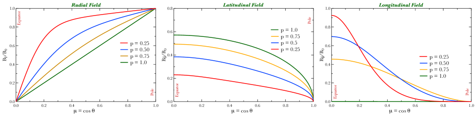
Figure 2: The $\,B_{\hat{r}}\,$, $\,B_{\hat{\theta}}\,$, and $\,B_{\hat{\phi}}\,$ components (from left to right) of the magnetic field in the Schwarzschild metric’s LIF at the surface of a $\,1.44M_{\odot}\,$ neutron star of radius $\,R_{\hbox{\sixrm NS}}=10^{6}\,$cm. They are plotted as functions of the magnetic colatitude $\,\mu=\cos{\theta}\,$ with $\,p=0.25,0.5,0.75\,$, and 1.0 (dark green, pure dipole case), ordered from top to bottom as indicated in the legends. The field component magnitudes are normalized by the field strength at the magnetic pole in the LIF, namely $\,B_{0}\approx 1.488B_{p}\,$.

One comparatively simple way to combine information from axisymmetric solutions of ideal MHD with general relativity is to directly embed the field components determined above in a magnetic field framework appropriate for the Schwarzschild metric, such as that developed in Petterson (1974); Wasserman & Shapiro (1983); Muslimov & Tsygan (1986) for dipole fields. In that dipolar configuration, the curved spacetime modifies the radial ($\,B_{r}\,$) and polar ($\,B_{\theta}\,$) field components by different analytic factors. These factors are described for the Schwarzschild geometry by the functions

$$\xi_{r}(\Psi) \;=\; -\frac{3}{\Psi^{3}}\left[\log_{e}(1-\Psi)+\Psi+\frac{\Psi^{2}}{2}\right]$$

$$\xi_{\theta}(\Psi) \;=\; \frac{6}{\Psi^{3}\sqrt{1-\Psi}}\left[(1-\Psi)\,\log_{e}(1-\Psi)+\Psi-\frac{\Psi^{2}}{2}\right],$$

where $\,\Psi=r_{\hbox{\sixrm S}}/r\,$ for a Schwarzschild radius $\,r_{\hbox{\sixrm S}}=2GM/c^{2}\,$. In the flat spacetime domain, $\,\xi_{r}\rightarrow 1\,$, $\,\xi_{\theta}\rightarrow 1\,$ when $\,\Psi\rightarrow 0\,$. Note that these definitions of $\,\xi_{r}\,$ and $\,\xi_{\theta}\,$ are scaled differently from those listed in Hu et al. (2019) and references therein.

The GR modification to the field components in the azimuthal and polar angle directions is identical, i.e., $\,\xi_{\phi}\equiv\xi_{\theta}\,$, an intuitive choice. The Schwarzschild geometry is invariant under rotations about the radial direction, and specifically so for 90 degree rotations that affect the coordinate mappings $\,\theta\leftrightarrow\pm\phi\,$. One deduces that the GR component amplification factors $\,\xi_{\phi}\,$ and $\,\xi_{\theta}\,$ are equal for any field configuration. For a mathematical determination of this identity for arbitrary multipoles, the reader can inspect Eqs. (5) and (6) of Muslimov & Tsygan (1986). Observe that the common enhancement factor $\,\xi_{\theta}\,$ cancels out when calculating the shear angle, so that Eq. (13) is still valid for our GR implementation. This symmetry does not extend to the Kerr metric.

The flat spacetime field components in Eq. (10) are then embedded in the Schwarzschild metric to generate $\,\bm{B}_{\rm GR}=(B_{{\hat{r}}},\,B_{{\hat{\theta}}},\,B_{{\hat{\phi}}})\,$, the LIF frame magnetic field (using the hat notation for LIF coordinates). Thus,

$$\bm{B}_{\rm GR}\;=\;\Bigl{[}\xi_{r}(\Psi)B_{rf},\;\xi_{\theta}(\Psi)B_{\theta f},\;\xi_{\theta}(\Psi)B_{\phi f}\Bigr{]}\quad,$$ (15)

where $\,B_{rf}\,$, $\,B_{\theta f}\,$ and $\,B_{\phi f}\,$ are the field components in flat spacetime, as specified in Eq. (9). This is the magnetic field form employed in the opacity calculations of this paper. Specific field loops can be computed numerically for a particular field line footpoint on the surface, or a maximum altitude $\,r_{\rm max}\,$, using parametric equations derived from the field components in the Schwarzschild metric:

$$\hbox{${{\displaystyle dr\vphantom{(}}\over{\displaystyle d\theta\vphantom{(}}}$}\;=\;r\sqrt{1-\Psi}\,\frac{B_{{\hat{r}}}}{B_{{\hat{\theta}}}}\quad\hbox{and}\quad\hbox{${{\displaystyle d\phi\vphantom{(}}\over{\displaystyle d\theta\vphantom{(}}}$}\;=\;\frac{1}{\sin{\theta}}\frac{B_{{\hat{\phi}}}}{B_{{\hat{\theta}}}}\quad.$$ (16)

This protocol was adopted for the visual depiction of the twisted field lines in Fig. 1, which were determined using $\,\Psi\approx 0.425\,$ for $\,M=1.44M_{\odot}\,$ and $\,R=10^{6}\,$cm.

Fig. 2 displays the different components of curved spacetime twisted magnetic field at the stellar surface. The field strengths are scaled by the zero-twist polar field strength $\,B_{0}=\xi_{r}(\Psi)\,B_{p}\,$ in the Schwarzschild metric, for $\,\Psi\approx 0.425\,$. For a fixed colatitude, the radial $\,B_{\hat{r}}\,$ component increases and the latitudinal (polar) $\,B_{\hat{\theta}}\,$ component decreases with decreasing $\,p\,$. The longitudinal (azimuthal) $\,B_{\hat{\phi}}\,$ component is more concentrated at $\,\mu=0\,$ with smaller $\,p\,$. When $\,p\,$ is small, the radial component dominates the magnetic field and asymptotically forms a split monopole. For magnetospheric regions beyond the stellar surface, all the components are simply multiplied by a factor of $\,(R_{\hbox{\sixrm NS}}/r)^{p+2}\,$, yet subject to different GR corrections, leaving the relative apportionment between the field components only mildly altered.

As an alternative approach, Kojima (2017) directly solved the Grad-Shafranov equation in the Schwarzschild metric, assuming an axisymmetric magnetosphere and a power-law form for the flux function. The GR metric modifications appear as modifiers to the various gradient operators embedded in the field’s vector potential, and a Legendre polynomial expansion in the $\,\mu=\cos\theta\,$ angular portion leads to radial eigenfunctions of hypergeometric function form. This protocol is more involved numerically than our choice here, and perhaps not as simple to digest. Yet it too generates an idealized solution through the parameterized power law assumption in specifying the toroidal $\,B_{\hat{\phi}}\,$ component. In reality, the expected restriction of zones of enhanced magnetization to flux tubes implies a caveat to all axisymmetric MHD models of neutron star magnetospheres. We adopt our protocol for its conceptual and numerical simplicity.

4 Escape Energies

In this section, the character of X-ray and gamma-ray escape energies is presented, for photons emitted at the stellar surface and in a magnetosphere described by the twisted field paradigm. After summarizing the opacity validation protocols, we consider three cases for emphasis. The first is where photons are emitted parallel to the local field direction; this is directly connected to the resonant inverse Compton scattering model of the persistent hard X-ray emission of magnetars. The next case of interest is for emission perpendicular to the local field, which approximately represents conditions most likely to be sampled in the bursts that are a common occurrence for magnetars. Finally, the focus turns to polar regions where the field line radii of curvature are large; this constitutes a case that may be quite relevant to the initial spikes of magnetar giant flares.

Our numerical calculations are validated by several methods. First, our photon trajectory integration is tested by comparing the integrated trajectories to the asymptotic trajectory formula presented in Poutanen (2020). The deviation of our computed light bending angles with that formula is around 0.003% for the worst case scenario where the photon is emitted horizontally from the stellar surface, i.e., at periastron. We compared the magnetic field strength and direction at select points along photon trajectories with analytic values for the cases with $\,p=0\,$ and $\,1\,$, yielding good agreement. The attenuation coefficient during the propagation of photons was plotted (not shown) as functions of pathlength and values checked at select positions along trajectories with the employed analytic forms for LIF values of the photon energy, the field strength and $\,\Theta_{\hbox{\sixrm kB}}\,$. Finally, calculated escape energies and opaque zones in the $\,p\rightarrow 1\,$ domain (green curves in Figures. 4 and 5) are in excellent agreement with the dipole results in Figures 5, 6, 9, and 10 in Hu et al. (2019), which also serve as checks of the opacity calculation.

4.1 Photons Emitted Parallel to B

The first case to be considered is when the photons are emitted parallel to the magnetic field at the point of emission. For magnetars, this closely matches the expectations of the popular resonant inverse Compton scattering (RICS) models for the production of their persistent hard X-ray emission above 10 keV (Baring & Harding, 2007; Fernández & Thompson, 2007; Beloborodov, 2013; Wadiasingh et al., 2018), discussed below. It is also relevant to curvature radiation emission components from high-field pulsars such as PSR B1509-58 (Harding, Baring & Gonthier, 1997), if they are generated by primary electrons accelerated in polar cap or slot gap potentials with $\,\bm{E}\cdot\bm{B}\neq 0\,$ in the inner magnetosphere (Daugherty & Harding, 1996; Muslimov & Harding, 2004).

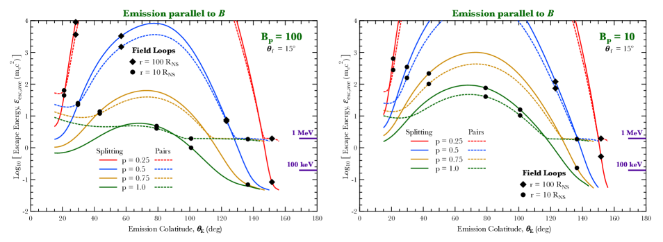
Figure 3: Polarization-averaged escape energies for photon splitting (solid curves) or pair creation (dashed curves) for photons emitted at points along twisted magnetic field loops with $\,p=0.25,\;0.5,\;0.75\,$ and $\,1.0\,$, ordered from top to bottom as indicated in the panel legends. The surface polar fields are $\,B_{p}=100\,$ and $\,B_{p}=10\,$ for the left and right panels, respectively. The footpoint colatitude $\,\theta_{\hbox{\sixrm f}}\,$ of the field loops is fixed at $\,15^{\circ}\,$, and photons start their trajectories parallel to the local field ($\,\Theta_{e}=0^{\circ}\,$). The black circles and diamonds label the colatitudes where the emission altitude equals $\,10R_{\hbox{\sixrm NS}}\,$ and $\,100R_{\hbox{\sixrm NS}}\,$, respectively. Short horizontal lines on the right-hand side of each panel indicate the energies of 1 MeV and 100 keV.

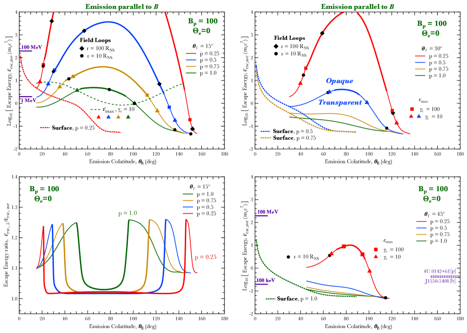
Figure 4: Escape energies for combined photon splitting and pair creation for photons emitted from the stellar surface (dashed curves) or along twisted magnetic field loops (solid curves) with $\,B_{p}=100\,$, and for $\,p=0.25,\;0.5,\;0.75\,$ and $\,1.0\,$, generally ordered from top to bottom (from outside to inside on the lower left) as indicated in the panel legends. Emission is parallel to the local field ($\,\Theta_{e}=0^{\circ}\,$). The heavyweight portion of the curves marks portions of the field lines where pair creation dominates photon splitting in determining the escape energy. The top and right panels depict the polarization-averaged escape energies for field loops with footpoint colatitudes $\,\theta_{f}=15^{\circ}\,$, $\,30^{\circ}\,$ and $\,45^{\circ}\,$ respectively. The bottom left panel displays the ratio of $\,\perp\,$ mode escape energy $\,\varepsilon_{\rm esc,\perp}\,$ to the polarization-averaged escape energy $\,\varepsilon_{\rm esc,ave}\,$ for $\,\theta_{f}=15^{\circ}\,$ that is depicted at the upper left. The colored triangles ($\,\gamma_{e}=10\,$) and squares ($\,\gamma_{e}=100\,$) represent the emission colatitude where the escape energy is equal to the maximum energy $\,\varepsilon_{\hbox{\sevenrm max}}\,$ produced by RICS (see Eq. 17 and associated text). The dashed green curve in the $\,\theta_{f}=15^{\circ}\,$ panel (upper left) defines the RICS $\,\varepsilon_{\hbox{\sevenrm max}}\,$ for the general relativistic dipole configuration ($\,p=1\,$). The filled black circles and diamonds label the locales on the field loops corresponding to an altitude equal to $\,10R_{\hbox{\sixrm NS}}\,$ and $\,100R_{\hbox{\sixrm NS}}\,$, respectively. In the lower right panel are marker energies (purple dashed lines) indicating the approximate maximum observed energy in two magnetars with polar fields somewhat close to the illustrated values, SGR J1550-5408 (bursts, [b]) and AXPs 4U 0142+61 (persistent emission, [p]); see Hu et al. (2019) for details concerning these observational indicators.

The opacity for a polarized photon emitted at a specific locale can be obtained using Eq. (1) with the attenuation coefficients of photon splitting and pair creation specified by Eqs. (5) and (8), respectively. Then the escape energy $\,\varepsilon_{\rm esc}\,$ is determined by adjusting the photon energy so that the cumulative optical depth in propagating to infinity equals unity, effectively a root solving algorithm for Eq. (2). Thus, $\,\varepsilon_{\rm esc}\,$ depends on the initial conditions, namely the emission position and direction, and subsequently also on the resultant path of the photon. Fig. 3 illustrates the escape energies $\,\varepsilon_{\rm esc}\,$ of photon splitting (solid) and pair creation (dashed) as functions of the emission colatitudes $\,\theta_{\hbox{\fiverm E}}\,$ for photons originating on specific field loops, with their initial photon momentum parallel to the local field, i.e. $\,\bm{k}\parallel\bm{B}\,$. Escape energies for combined photon splitting and pair creation with surface polar fields $\,B_{p}=100\,$ and $\,B_{p}=10\,$ are illustrated in Figs. 4 and 5, respectively. The escape energy loci in both of these Figures were determined for field loops with one of the footpoint colatitudes located at $\,\theta_{\hbox{\sixrm f}}=15^{\circ}\,$, and for four different twist parameter $\,p\,$ values. On each curve in Fig. 3, the black circles and diamonds mark the colatitudes where the emission locales have radii of 10 and 100 $\,R_{\hbox{\sixrm NS}}\,$ respectively. Decreasing the $\,p\,$ value enlarges the field loop so that its maximum altitude is larger (see Table 1), corresponding to much larger radii of field curvature on average.

= 20mm $\,r_{\hbox{\sevenrm max}}\;(R_{\hbox{\sixrm NS}})\,$ $\,p\,$ $\,\theta_{\hbox{\sixrm f}}=15^{\circ}\,$ $\,\theta_{\hbox{\sixrm f}}=30^{\circ}\,$ $\,\theta_{\hbox{\sixrm f}}=45^{\circ}\,$ $\,\theta_{\hbox{\sixrm f}}=60^{\circ}\,$ 1.00 10.37 3.01 1.67 1.22 0.75 29.92 5.29 2.22 1.38 0.50 266.5 18.12 4.30 1.84 0.25 2.13$\,\times 10^{5}\,$ 909.6 42.48 5.69

Table 1: $\,\theta_{\hbox{\sixrm f}}-r_{\hbox{\sevenrm max}}\,$ relations for different $\,p\,$ values

The field loop escape energies in Fig. 3 are maximized at colatitudes somewhat smaller than $\,90^{\circ}\,$, and resemble the bell-shaped behavior presented in Fig. 10 of Hu et al. (2019) ($\,p=1\,$ case only). This is expected because of the high altitudes of emission at quasi-equatorial colatitudes, where the magnetic fields are relatively weak. Pair creation dominates the attenuation and determines the escape energy at colatitudes remote from the footpoints, and these domains are marked as heavyweight portions of the curves in Fig. 4 (upper left); the lower average fields along the photon trajectories tend to favor the dominance of pair conversion over photon splitting once the energy threshold is exceeded (e.g., Baring & Harding, 2001). While the pair conversion escape energies (for an observer at infinity) in Fig. 3 generally exceed the threshold of $\,2m_{e}c^{2}\,$ for pair creation, there are noticeable portions near the highest emission colatitudes where values slightly lower than $\,2m_{e}c^{2}\,$ are apparent. These correspond to inward emission cases where the LIF frame photon energy actually exceeds the pair threshold for the inner portion (near periastron) of the trajectory to infinity. For both processes, the escape energy curves are asymmetric about the equator ($\,\theta_{\hbox{\fiverm E}}=90^{\circ}\,$), since photons emitted from upper and lower hemispheres possess different trajectories. Photons emitted outward travel to regions of lower field magnitudes and larger radii of curvature. In contrast, those emitted inward sample fields that are stronger and field lines that are more highly curved (see the sample trajectories in Fig. 9), conditions conducive to greater opacity, thereby lowering $\,\varepsilon_{\rm esc}\,$.

The key feature of the impact of twists to the magnetospheric geometry is that the escape energy for loop emission increases as $\,p\,$ decreases. This is caused by two effects. At small colatitudes, decreasing $\,p\,$ enhances the radial $\,B_{\hat{r}}\,$ component. Thus the initial photon momentum $\,\bm{k}\,$ is typical more radial than it is in a dipole field, and $\,\Theta_{\hbox{\sixrm kB}}\,$ increases more slowly for lower $\,p\,$ due to the straighter field lines, unless the photon is very far from the stellar surface. For moderate colatitudes, decreasing $\,p\,$ raises the emission locale to a higher altitude (see the black circles and diamonds in Fig. 4), which also reduces the opacity as the typical value of $\,|\bm{B}|\,$ along the trajectory is lower. Accordingly, the higher the axisymmetric MHD twist, the more transparent the magnetosphere becomes to splitting and pair creation for photons emitted parallel to $\,\bm{B}\,$ along field lines. As $\,p\,$ declines, the opacities should rise with the increase of the field magnitude $\,|\bm{B}|\,$ that is evident in Fig. 2. Yet, this influence is actually dominated by the associated increase in the radii of field line curvature for higher twists, which reduces the magnetospheric opacity as the field morphology progresses towards that of a split monopole.

Escape energies for photons emitted from the stellar surface are also depicted in Fig. 4 as dashed curves. These curves start at $\,\theta_{\hbox{\fiverm E}}=0^{\circ}\,$ and decrease with the increase of $\,\theta_{\hbox{\fiverm E}}\,$ because the field line curvature radii are smaller at non-polar colatitudes. All the curves are truncated at $\,\theta_{\hbox{\fiverm E}}=90^{\circ}\,$, beyond which the emitted photons propagate inward and therefore never enter the magnetosphere. The escape energy curves for the loop emission touch the surface curves at the footpoint colatitudes $\,\theta_{\hbox{\sixrm f}}\,$, where the field loops are anchored at the surface. The escape energies for surface emitted photons also increase with the decrease of $\,p\,$, observing that the initial photon momentum $\,\bm{k}\,$ is more radially directed when $\,p\,$ is small.

The resonant upscattering of the surface thermal emission by relativistic $\,e^{+}/e^{-}\,$ is very efficient in the magnetospheres of magnetars, because the resonance at the cyclotron frequency ($\,\varepsilon=B\,$) increases the cross section by around 2-3 orders of magnitude above the classical Thomson value when $\,B\mathrel{\mathchoice{\lower 2.0pt\vbox{\halign{$\m@th\displaystyle\hfil#\hfil$\cr<\crcr\sim\crcr}}}{\lower 2.0pt\vbox{\halign{$\m@th\textstyle\hfil#\hfil$\cr<\crcr\sim\crcr}}}{\lower 2.0pt\vbox{\halign{$\m@th\scriptstyle\hfil#\hfil$\cr<\crcr\sim\crcr}}}{\lower 2.0pt\vbox{\halign{$\m@th\scriptscriptstyle\hfil#\hfil$\cr<\crcr\sim\crcr}}}}1\,$ (e.g., Gonthier et al., 2000). The velocity of the ultra-relativistic $\,e^{+}/e^{-}\,$ (Baring & Harding, 2007; Wadiasingh et al., 2018) is essentially parallel to the magnetic field direction due to rapid cyclotron cooling perpendicular to the field, modulo small drift velocity components due to the slow magnetar rotation. Thus the momentum of the upscattered photon is nearly parallel to the magnetic field as a consequence of Doppler beaming. This also applies to other emission mechanisms, including curvature radiation and synchrotron emission for $\gamma$-ray pulsars. The scattered $\,e^{+}/e^{-}\,$ are assumed to stay in the ground Landau states, which is relevant to situations where the scattering samples energy near or below the fundamental cyclotron resonance. This is generally valid due to rapid cooling of $\,e^{+}/e^{-}\,$ near the cyclotron resonance, which can normally prevent $\,e^{+}/e^{-}\,$ from encountering higher cyclotron harmonics; see Baring et al. (2011) for a discussion.

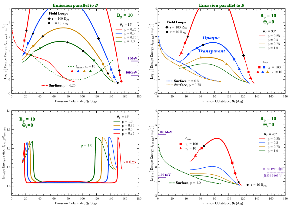
Figure 5: Escape energies for photon splitting and pair creation for photons emitted from the stellar surface (dashed curves) or along twisted magnetic field loops (solid curves). Again, these are for $\,p=0.25,\;0.5,\;0.75\,$ and $\,1.0\,$, being ordered generally from top to bottom (or from outside to inside on the lower left) as indicated in the panel legends. The surface polar field is now $\,B_{p}=10\,$, and emission is again parallel to the local field ($\,\Theta_{e}=0^{\circ}\,$). Labels for points in all panels are identical to those in Fig. 4, as are the observational data markers in the lower right panel.

For this case of scatterings being dominated by those sampling the cyclotron frequency, the maximum scattered photon energy $\,\varepsilon_{\hbox{\sevenrm max}}\,$ is realized for a head-on collision with a photon scattering angle of $\,180^{\circ}\,$ in the electron rest frame, which leads to (Baring et al., 2011)

$$\vspace{-5pt}\varepsilon_{\hbox{\sevenrm max}}\;=\;\gamma_{e}(1+\beta_{e})\left(\frac{B}{1+2B}\right)\quad.$$ (17)

Here $\,\gamma_{e}\,$ is the Lorentz factor of the $\,e^{+}/e^{-}\,$, $\,\beta_{e}\,$ is the ratio of lepton speed to $\,c\,$, and $\,B\,$ is the field strength at the scattering locale. This form was employed in Hu et al. (2019) in Fig. 8 for the dipole case. For fixed lepton velocity, the maximum scattered photon energy $\,\varepsilon_{\hbox{\sevenrm max}}\,$ solely depends on the field strength, and obviously saturates at $\,\gamma_{e}(1+\beta_{e})/2\,$ when $\,B\gg 1\,$.

The gravitational-redshifted maximum scattered photon energy $\,\varepsilon_{\hbox{\sevenrm max}}/(\sqrt{1-\Psi})\approx 1.32\varepsilon_{\hbox{\sevenrm max}}\,$ (for $\,\Psi=0.425\,$) along the $\,p=1\,$ field loop is displayed as a sparsely dashed green curve in the upper left panel of Fig. 4. This is specifically for a fixed $\,\gamma_{e}=10\,$, a value that naturally emerges as a result of rampant RICS cooling (Baring et al., 2011; Wadiasingh et al., 2018) in magnetar-strength fields. The $\,\varepsilon_{\hbox{\sevenrm max}}\,$ trace is symmetric about the magnetic equator ($\,\theta_{\hbox{\fiverm E}}=90^{\circ}\,$), and it intersects the escape energy curve at $\,\theta_{\hbox{\fiverm E}}\approx 50^{\circ},100^{\circ}\,$, which are labeled by green triangle markers. At low/high colatitudes outside these two intersections, the maximum photon energy $\,\varepsilon_{\hbox{\sevenrm max}}\,$ is larger than the escape energy $\,\varepsilon_{\rm esc}\,$, therefore photon splitting will attenuate the highest energies of hard X-ray photons produced by RICS. The $\,\varepsilon_{\hbox{\sevenrm max}}\,$ curves for field loops with smaller $\,p\,$ values share similar behavior and so are not displayed in the figures. The $\,\varepsilon_{\hbox{\sevenrm max}}\,$ values decline along the trace as the colatitude moves away from the poles towards the equator because the emission locales are then farther from the surface and the field strength is weaker. Intersections of loci for $\,\varepsilon_{\hbox{\sevenrm max}}\,$ and $\,\varepsilon_{\rm esc}\,$ for loops with different $\,p\,$ values are labeled in the figures with triangle markers ($\,\gamma_{e}=10\,$) and square markers ($\,\gamma_{e}=100\,$) in the three panels that depict escape energies. The separation of the two intersection points increases with a decrease of $\,p\,$, so that when $\,p\,$ is small, photon splitting is more likely to attenuate photons at energies below $\,\varepsilon_{\hbox{\sevenrm max}}\,$ near the field line footpoints.

The bottom-left panel of Fig. 4 illustrates the ratio of the $\,\perp\,$ mode ($\,\perp\rightarrow\parallel+\parallel\,$, $\,\perp\rightarrow e^{+}e^{-}\,$) escape energy to the polarization-averaged escape energy. The ratios increase with emission colatitude $\,\theta_{\hbox{\fiverm E}}\,$ at small $\,\theta_{\hbox{\fiverm E}}\,$; and sharply drop to around unity when pair creation dominates the opacities (the heavyweight portion demarcates pair conversion dominance for $\,\varepsilon_{\rm esc,\perp}\,$) at quasi-equatorial colatitudes. For the quasi-polar domains where photon splitting determines the escape energy, the ratio can be intuitively estimated as $\,\varepsilon_{\rm esc,\perp}/\varepsilon_{\rm esc,ave}\approx\left[2{\cal M}_{1}^{2}/(3{\cal M}_{1}^{2}+{\cal M}_{2}^{2})\right]^{-1/5}\,$. This approaches the value $\,(338/1083)^{-1/5}\approx 1.26\,$ in the sub-critical field domain, which is in agreement with the ratio cusps apparent in Fig. 4. For pair creation considerations, the escape energy ratio can be estimated assuming $\,3\exp{[-8/(3B\varepsilon_{\rm esc,ave})}]/2\approx\exp{[-8/(3B\varepsilon_{\rm esc,\perp})}]\,$ in the sub-critical field domain. This estimate is obtained using the asymptotic expressions for the polarization-dependent and polarization-averaged pair creation rates in Erber (1966), which can also be deduced by taking the $\,\varepsilon_{\perp}\gg 2\,$ limit of the expressions in Eq. (23) in Appendix A. This relation yields $\,\varepsilon_{\rm esc,\perp}/\varepsilon_{\rm esc,ave}\approx 1+3B\varepsilon_{\rm esc}\ln{(3/2)}/8\approx 1+0.152B\varepsilon_{\rm esc}\,$, which is very close to unity for high altitude emission near the equator. Since these ratios are not vastly different from unity, it is sufficient to employ just polarization-averaged opacity determinations for deriving the representative character of opacity in the ensuing exposition.

Fig. 5 is a $\,B_{p}=10\,$ analogue of the escape energy results in Fig. 4. This value is close to the surface field strengths of most magnetars. Since the attenuation of both photon splitting and pair creation is positively correlated with the field strength, the escape energies are generally higher than those in Fig. 4. So the domination of pair creation (weighted curves) covers a larger portion of the escape energy curves. Yet the general shapes of the escape energy curves are quite similar to those in Fig. 4, a consequence of the employment of an identical selection of field morphologies.

4.2 Photons Emitted Perpendicular to B

Modest or large emission angles $\,\Theta_{\hbox{\sixrm e}}\,$ to the local field are expected for magnetar bursts and flares, where radiation comes from highly optically-thick “fireballs” along magnetic flux tubes populated by quasi-thermalized electron-positron pair plasma. To accommodate this situation and provide a contrast to results from Section 4.1, we explore the escape energy for photons emitted initially perpendicular to the local $\,\bm{B}\,$ field, which might be the primary direction for radiation to escape from the fireball in the closed-field region. Here we consider four different azimuthal directions for such $\,\Theta_{\hbox{\sixrm e}}=90^{\circ}\,$ cases, namely primarily outward emission ($\,\bm{k}\propto\bm{B}\times\hat{\phi}\,$ so that $\,\bm{k}\cdot\hat{r}>0\,$), inward emission ($\,\bm{k}\propto\hat{\phi}\times\bm{B}\,$ with $\,\bm{k}\cdot\hat{r}<0\,$) both in the $\,r-\theta\,$ planes, and two sideways emission cases [$\,\pm\bm{k}\propto(\bm{B}\times\hat{\phi})\times\bm{B}\,$] that are essentially orthogonal to active magnetic flux tubes.

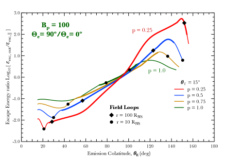
Figure 6: The ratio of the escape energies (logarithmic scale) of photons emitted perpendicular to the local B direction ($\,\Theta_{\rm e}=90^{\circ}\,$) to those emitted parallel to the field ($\,\Theta_{\rm e}=0^{\circ}\,$). These ratios are plotted as functions of the emission colatitude on field loops with a fixed footpoint colatitude of $\,\theta_{\hbox{\sixrm f}}=15^{\circ}\,$, for four different $\,p\,$ values, as indicated. For the perpendicular emission, the initial photon momentum satisfied $\,\bm{k}\propto\bm{B}\times\hat{\phi}\,$ (outward). The heavy-weight portions of the curves represent the locales where the attenuation of outward emitted photons is dominated by pair creation. The black circles and diamonds label the colatitudes associated with radii equal 10$\,R_{\hbox{\sixrm NS}}\,$ and 100$\,R_{\hbox{\sixrm NS}}\,$, respectively.

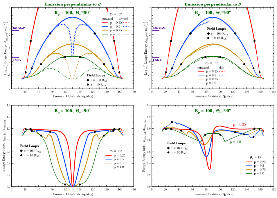
Figure 7: Upper panels: escape energies for photon splitting and pair creation for emission on twisted magnetic field loops, $\,p=0.25,\;0.5,\;0.75\,$ and $\,1.0\,$, ordered from top to bottom as indicated in the legends. Here $\,B_{p}=100\,$, and emission is perpendicular to the local field ($\,\Theta_{e}=90^{\circ}\,$). Solid curves address photons generally emitted outward ($\,\bm{k}\propto\bm{B}\times\hat{\phi}\,$, giving $\,\varepsilon_{\rm esc,out}\,$), while the dashed curves therein display the escape energies for (a) inward-directed photons ($\,\bm{k}\propto\hat{\phi}\times\bm{B}\,$, giving $\,\varepsilon_{\rm esc,in}\,$) on the left, and (b) sideways emission cases ($\,\varepsilon_{\rm esc,side}\,$ for $\,\bm{k}\propto[\bm{B}\times\hat{\phi}]\times\bm{B}\,$). The two lower panels display the ratios $\,\varepsilon_{\rm esc,in}/\varepsilon_{\rm esc,out}\,$ (left) and $\,\varepsilon_{\rm esc,side}/\varepsilon_{\rm esc,out}\,$ (right). Again, heavyweight curves mark the colatitudes where attenuation is dominated by pair creation, and the black circles and diamonds mark the colatitudes where the radii equal 10$\,R_{\hbox{\sixrm NS}}\,$ and 100$\,R_{\hbox{\sixrm NS}}\,$, respectively.

To benchmark the ensuing depictions against the results displayed in Figs. 4 and 5, the ratios of escape energies of outward emission cases to parallel emission cases are displayed in Fig. 6 for four different $\,p\,$ values and a fixed $\,\theta_{\hbox{\sixrm f}}=15^{\circ}\,$. Note the logarithmic representation of the ratios, employed because they span around 5 decades in range. The weighted portion of the curves marks the outward emission locales from where photon attenuation is dominated by pair creation instead of photon splitting. The ratio is smaller than unity for emission colatitude $\,\theta_{\hbox{\fiverm E}}<90^{\circ}\,$ and larger than unity for $\,\theta_{\hbox{\fiverm E}}>90^{\circ}\,$. For $\,\theta_{\hbox{\fiverm E}}<90^{\circ}\,$, at the emission local $\,\Theta_{\hbox{\sixrm kB}}\equiv\Theta_{\hbox{\sixrm e}}=90^{\circ}\,$ for outward-moving photons, and the escape energy is markedly reduced relative to the situation where emission is locally parallel to $\,\bm{B}\,$. For emission colatitudes $\,\theta_{\hbox{\fiverm E}}>90^{\circ}\,$ in the other hemisphere, parallel emitted photons travel close to the stellar surface where the field strength is strong. Yet the $\,\Theta_{\hbox{\sixrm e}}=90^{\circ}\,$ photons still propagate outwards into weaker fields, with trajectories that are symmetric about the magnetic equator, i.e. under the interchange $\,\theta_{\hbox{\fiverm E}}\to 180^{\circ}-\theta_{\hbox{\fiverm E}}\,$. The combination of these influences leads the escape energy ratio to generally be an increasing function of $\,\theta_{\hbox{\fiverm E}}\,$. The deviation of the escape energy ratio from unity at small and large colatitudes is enhanced for small $\,p\,$, primarily because the radial component of the photon momentum vector is enhanced with larger twists for the case of photons emitted parallel to $\,\bm{B}\,$.

Fig. 7 illustrates the escape energies for photons emitted perpendicular to field loops that are characterized by footpoint colatitude $\,\theta_{\hbox{\sixrm f}}=15^{\circ}\,$ and four different $\,p\,$ values. In the top two panels, the solid curves represent the outward emission case where photons possess initial momenta $\,\bm{k}\propto\bm{B}\times\hat{\phi}\,$ and propagate away from the star. The escape energies for the inward case ($\,\bm{k}\propto-\bm{B}\times\hat{\phi}\,$) are displayed in the upper left panel as dashed curves. For both emitting directions, the photon trajectories lie in “meridional” $\,(r,\theta)\,$ planes so that the escape energy curves are symmetric about the magnetic equator. The outward emission escape energy curves resemble the bell shapes in the parallel emitting case, with ratios of the two as depicted in Fig. 6. For the inward case, the photon escape energy is strongly diminished near the equator, generating a double-peaked shape. This reduction is because the trajectories of these photons pass close to the stellar surface; the gaps in the inward curves demarcate the locales where emitted photons actually hit the star. These colatitudes of stellar shadowing of the radiation get reduced as the twist increases since the equatorial portions of the loops move to higher altitudes, for which the star becomes more remote. The cusps in the $\,p=1\,$ outward emission curves near $\,\theta_{\hbox{\fiverm E}}=72^{\circ}\,$ and 108$\,{}^{\circ}\,$ are caused by the fact that pair creation attenuation coefficient is not a strictly increasing function of photon energy between two distinctive Landau levels. Thus the escape energy exhibits two small steps which correspond to the first and second Landau levels (see Appendix A).

Escape energy curves for photons emitted in one of the sideways directions [$\,\bm{k}\propto(\bm{B}\times\hat{\phi})\times\bm{B}\,$] are displayed as dashed curves on the upper right of Fig. 7. The curves are now not symmetric about the equator, and the values of the escape energy are intermediate between those of the outward and inward emission cases. The escape energies for another side direction [$\,-\bm{k}\propto(\bm{B}\times\hat{\phi})\times\bm{B}\,$] are reflection-symmetric about the equator to the depicted ones, and thus they are not explicitly displayed.

To complete the suite of information, the escape energy ratios $\,\varepsilon_{\rm esc,in}/\varepsilon_{\rm esc,out}\,$ and $\,\varepsilon_{\rm esc,side}/\varepsilon_{\rm esc,out}\,$ are presented in the lower panels of Fig. 7. This row augments the upper panel information wherein it is difficult to discern escape energy curves that differ by 10% or less. The $\,\varepsilon_{\rm esc,in}/\varepsilon_{\rm esc,out}\,$ ratios are close to unity for large or small emission colatitudes and drop to around zero near the equator. As the twist increases, the emission locale raises and the ratio drops arise at colatitudes somewhat closer to the equator. Therefore the differences between outward and inward emission cases decrease with higher field twists. The $\,\varepsilon_{\rm esc,side}/\varepsilon_{\rm esc,out}\,$ ratios also decline near the equator. The equatorial bump in the $\,p=1\,$ case is caused by the onset of pair creation in the outward emission case. Curve structure bracketing the bump, with analogous variations exhibited for other $\,p\,$ values (albeit less pronounced), captures the discontinuities of the pair conversion rates near threshold; see Appendix A. The shapes of the $\,\varepsilon_{\rm esc,side}/\varepsilon_{\rm esc,out}\,$ ratios are generally complicated since photons emitted sideways do not move in fixed $\,(r,\theta)\,$ planes. Yet the ratios are generally close to unity (20%) for most emission colatitudes.

In summary, the main message contained in the results depicted in Figs. 6 and 7 is that emitting photons at large angles to the local field alters the magnetospheric opacity substantially, and that the escape energy is most sensitive to the azimuthal direction of emission around $\,\bm{B}\,$ for equatorial locales. Both these properties emerge naturally from the angle and field dependence of the pair creation and photon splitting rates.

4.3 Polar Emission Zones

The final focus of our results section is on the regions very close to the magnetic poles. This is primarily motivated by the phenomena of magnetar giant flares, yet it may also be germane (Younes et al., 2021) to the simultaneous detection of a fast radio burst (FRB; Bochenek et al., 2020) with a hard X-ray one (FRB-X; Mereghetti et al., 2020; Ridnaia et al., 2021) from the magnetar SGR 1935+2154 on April 28 (UTC), 2020.

Transient giant flares possess enormous luminosities $\,10^{44}-10^{47}\,$ erg/sec at hard X-ray energies, and constitute the hardest emission signal known for magnetars. Their initial spikes, generally lasting less than around 0.2 sec, are observed to extend up to the MeV-band energies that permit pair creation to possibly be active. Specifically, for the Galactic magnetar giant flares, Hurley et al. (1999a) identified emission up to around 2 MeV for the August 27, 1998 event from SGR 1900+14, while Hurley et al. (2005) reported signals up to around 1 MeV for the December 27, 2004 giant flare from SGR 1806-20. Going beyond the Milky Way, the April 15, 2020 giant flare from a magnetar in the NGC 253 galaxy was far enough away that only the initial spike was observed, and it was not subject to instrumental saturation influences. This event thus supplied unprecedented time-resolved spectroscopy. Fermi-GBM observations of the transient detected photons up to around 3 MeV (Roberts et al., 2021), and the interpretation was that the initial spike constituted soft gamma-ray emission from relativistic plasma outflow from the polar (perhaps open field-line) regions of a rotating magnetar. This picture motivates the focal investigation of this subsection.

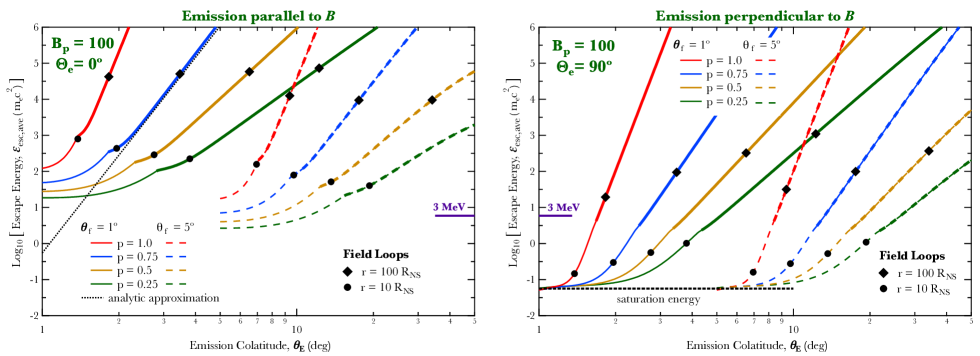
Figure 8: Left: Polarization-averaged escape energies plotted as functions of emission colatitude $\,\theta_{\hbox{\fiverm E}}\,$ (note the logarithmic scale) for photons emitted parallel to the local field directions ($\,\Theta_{e}=0^{\circ}\,$) from field loops with footpoint colatitudes $\,\theta_{\hbox{\sixrm f}}=1^{\circ}\,$ (solid) and $\,\theta_{\hbox{\sixrm f}}=5^{\circ}\,$ (dashed) for four different $\,p\,$ values. As in prior figures, the black circles and diamonds mark the colatitudes where the emission altitude equals 10 $\,R_{\hbox{\sixrm NS}}\,$ and 100 $\,R_{\hbox{\sixrm NS}}\,$, respectively. The black dotted curve is the escape energy for the $\,p=0.5\,$ case calculated using the analytic formula in Eq. (18), with $\,\theta_{\hbox{\sixrm f}}\,$ adjusted to accommodate the increase of the field line footpoint colatitude in curved spacetime. Right: Escape energies for photons emitted perpendicular to the local field directions ($\,\Theta_{e}=90^{\circ}\,$, outward-directed, i.e., $\,\bm{k}\propto\bm{B}\times\hat{\phi}\,$) from field loops anchored at $\,\theta_{\hbox{\sixrm f}}=1^{\circ}\,$ (solid) and $\,\theta_{\hbox{\sixrm f}}=5^{\circ}\,$ (dashed). The horizontal dashed line indicates the asymptotic escape energy [$\,\approx 26\,$keV; see Eq. (20) and the related text].

For the polar surface field $\,B_{p}=100\,$ case, Fig. 8 displays the escape energies for photons emitted parallel to the local magnetic field directions from field loops anchored at polar regions, specifically with $\,\theta_{\hbox{\sixrm f}}=1^{\circ}\,$ and $\,5^{\circ}\,$. The left panel partners three of the panels in Fig. 4, while the right panel is to be compared with the solid curves in the upper panels of Fig. 7. In both cases, the escape energies increase with the emission colatitude $\,\theta_{\hbox{\fiverm E}}\,$ and realize power laws when pair production is the dominant mode of photon attenuation, corresponding to emission altitudes larger than around 10 $\,R_{\hbox{\sixrm NS}}\,$. This is a domain where the GR influences are small, so that a flat-spacetime asymptotic analysis can be used to describe the analytic character of the escape energy. For the emission parallel to $\,\bm{B}\,$, the case in the left panel, this adapts the protocol developed by Story & Baring (2014). The power-law behavior can be well estimated by an analytic approximation:

$$\varepsilon_{\rm esc}\;\approx\;A(p)\frac{h^{2+p/2}}{B_{p}\theta_{\hbox{\sixrm f}}}\;\approx\;A(p)\frac{\theta_{\hbox{\fiverm E}}^{1+4/p}}{B_{p}\theta_{\hbox{\sixrm f}}^{2+4/p}}\quad,$$ (18)

where the poloidal field line relation in Eq. (26) is used in the second approximation, and

$$A(p) \;=\;\frac{2^{5}(p+3)^{p+3}}{3p(p+2)^{p+3}}$$ (19)

$$\times\left\{\log{\left[\frac{3^{2}p(p+2)^{3p/2+5/2}}{2^{8}(p+3)^{3p/2+4}}\frac{\alpha_{\hbox{\sevenrm f}}R_{\hbox{\sixrm NS}}}{\lambdabar_{c}}\right]}\right\}^{-1}\;.$$

Here $\,h=r/R_{\hbox{\sixrm NS}}\,$ is the altitude of the emission locale scaled by the stellar radius $\,R_{\hbox{\sixrm NS}}\,$. This relation is an extension of the Eq. (20) of Story & Baring (2014) to the twisted field configuration. It is valid for arbitrary twist parameter $\,0<p\leq 1\,$ with $\,\theta_{\hbox{\fiverm E}}\ll\,$ 1. For a specific $\,p\,$, one can infer that $\,\varepsilon_{\rm esc}\propto h^{2+p/2}\propto\theta_{\hbox{\fiverm E}}^{1+4/p}\,$, with a power-law index that is independent of the field strength $\,B_{p}\,$ and the footpoint colatitude $\,\theta_{\hbox{\sixrm f}}\,$ of the field loops. The derivation of Eq. (18) is detailed in Appendix B. Eq. (18) is plotted for $\,p=0.5\,$ and $\,\theta_{\hbox{\sixrm f}}=1^{\circ}\,$ as the black dotted curve in Fig. 8 to compare with the numerical results. Although not depicted in the figure, Eq. (18) well approximates (with error $\,\mathrel{\mathchoice{\lower 2.0pt\vbox{\halign{$\m@th\displaystyle\hfil#\hfil$\cr<\crcr\sim\crcr}}}{\lower 2.0pt\vbox{\halign{$\m@th\textstyle\hfil#\hfil$\cr<\crcr\sim\crcr}}}{\lower 2.0pt\vbox{\halign{$\m@th\scriptstyle\hfil#\hfil$\cr<\crcr\sim\crcr}}}{\lower 2.0pt\vbox{\halign{$\m@th\scriptscriptstyle\hfil#\hfil$\cr<\crcr\sim\crcr}}}}30\%\,$ for $\,\theta_{\hbox{\fiverm E}}\mathrel{\mathchoice{\lower 2.0pt\vbox{\halign{$\m@th\displaystyle\hfil#\hfil$\cr<\crcr\sim\crcr}}}{\lower 2.0pt\vbox{\halign{$\m@th\textstyle\hfil#\hfil$\cr<\crcr\sim\crcr}}}{\lower 2.0pt\vbox{\halign{$\m@th\scriptstyle\hfil#\hfil$\cr<\crcr\sim\crcr}}}{\lower 2.0pt\vbox{\halign{$\m@th\scriptscriptstyle\hfil#\hfil$\cr<\crcr\sim\crcr}}}}20^{\circ}\,$ and $\,h>10\,$) the power-law relationships for all the other $\,p\,$ cases. Observe that there is a slight downward curvature at high colatitudes beyond the $\,\theta_{\hbox{\fiverm E}}\ll 1\,$ domain.

The right panel of Fig. 8 illustrates the escape energies for photons emitted perpendicular (outward-directed with $\,\bm{k}\propto\bm{B}\times\hat{\phi}\,$) to the field loops for the same polar footpoint colatitudes. Note that the escape energies for other perpendicular emission cases (inward-directed, sideways) are almost identical to the outward case. The values of the escape energies are smaller than their counterparts for the parallel emission case, since photons immediately move across field lines, thereby manifesting a different power-law behavior with $\,\varepsilon_{\rm esc}\propto\theta_{\hbox{\fiverm E}}^{2+4/p}\,$. This index can be quickly obtained by inserting $\,\Theta_{\hbox{\sixrm kB}}=\pi/2\,$, $\,B\propto B_{p}/h^{p+2}\,$, and Eq. (26) into $\,B\omega_{\perp}\approx\,$ constant; similar behavior is realized for other fixed values of $\,\Theta_{\hbox{\sixrm kB}}\,$.

The escape energy curves also realize a horizontal saturation (black dashed line) at small emission colatitudes $\,\theta_{\hbox{\fiverm E}}\,$ close to the stellar surface. The saturated escape energy is independent of the twist parameter $\,p\,$, and can be estimated in a superstrong field where $\,{\cal M}_{1}\approx 1/(6B^{3})\,$ dominates the reaction rates $\,{\cal M}_{\sigma}\,$ (see Eqs. 6 and LABEL:eq:Lambda_s_def) and the photon splitting coefficient is independent of the field strength. In this case, Eq. (5) yields

$$\varepsilon_{\rm esc}\;\approx\;\sqrt{1-\Psi_{\hbox{\sixrm E}}}\left(\frac{1440\pi^{2}\lambda\hbox to0.0pt{\hss--}_{c}}{\alpha_{\hbox{\sevenrm f}}^{3}R_{\hbox{\sixrm NS}}\,\sin^{6}\Theta_{\hbox{\sixrm e}}}\right)^{1/5}\quad.$$ (20)

Here we assume that the stellar radius $\,R_{\hbox{\sixrm NS}}\,$ is the typical lengthscale for the attenuation. For emission locales near the surface, Eq. (20) gives a saturated escape energy $\,\varepsilon_{\rm esc}\approx 26\,$ keV when $\,\Theta_{\hbox{\sixrm e}}=\pi/2\,$ and $\,\Psi_{\hbox{\sixrm E}}=0.425\,$, which is in agreement with the values near the footpoint colatitudes for both $\,\theta_{f}=1^{\circ}\,$ and $\,5^{\circ}\,$ in the right panel of Fig. 8. For $\,\Theta_{\hbox{\sixrm e}}<\pi/3\,$, the typical attenuation locales are well removed from the surface, and then Eq. (20) accurately expresses the saturation energy when $\,\Psi_{\hbox{\sixrm E}}\to 0\,$ and $\,\varepsilon_{\rm esc}\approx 36\,\hbox{keV}\,(\sin\Theta_{\hbox{\sixrm e}})^{-6/5}\,$.

A key feature of the polar region emission is that the escape energy for parallel emitted photons increases with the decrease of the field loop footpoint colatitude $\,\theta_{\hbox{\sixrm f}}\,$, for fixed field strength $\,B_{p}\,$ and twist parameter $\,p\,$. Therefore in the polar region, the escape energy can be very large ($\,>10-100\,$MeV) even for photons emitted near the surface, since the field lines are only mildly curved. Adding twists to the field configuration will further enlarge the escape energy because the radius of the curvature is increased. According to Fig. 8, this is more pronounced for the case of emission parallel to $\,\bm{B}\,$, much less so for emission orthogonal to the field. This rise in $\,\varepsilon_{\rm esc}\,$ as $\,\theta_{\hbox{\sixrm f}}\,$ becomes small applies to both processes, so that the competition between pair creation and photon attenuation in polar regions appears to be only modestly dependent on the twist parameter $\,p\,$.

The 3 MeV energy markers on both panels of Fig. 8 signify the approximate maximum energy observed from the initial spike of the magnetar giant flare in the NGC 253 galaxy (Roberts et al., 2021) by Fermi-GBM in 2020. It is clear from the left panel of Fig. 8 that photon transparency in the inner magnetosphere for such a signal is guaranteed right down to the surface if the pertinent field line footpoint colatitude is somewhat smaller than $\,5^{\circ}\,$, and the emission is along the field. In striking contrast, if the emission is perpendicular to the field, and outward directed (right panel), then photon splitting and even pair creation would be rife, precluding the visibility of such a signal if generated at altitudes of $\,30R_{\hbox{\sixrm NS}}\,$ or less. The $\,\varepsilon_{\rm esc}\,$ curves are very similar for inward-directed, $\,\Theta_{\hbox{\sixrm e}}=\pi/2\,$ emission (not displayed). Moreover, our computed saturation escape energies for photon splitting are 295 keV for $\,\Theta_{\hbox{\sixrm e}}=10^{\circ}\,$ and 674 keV for $\,\Theta_{\hbox{\sixrm e}}=5^{\circ}\,$ for all axisymmetric twist scenarios; see Eq. (20). While Doppler boosting will likely beam the hardest giant flare emission along the local field, substantial angles $\,\Theta_{\hbox{\sixrm e}}\,$ to the field will be germane to emission at energies below 1 MeV. Accordingly, the time-dependent spectra presented in Roberts et al. (2021) likely constrains the inferred quasi-polar emission altitude to at least $\,10R_{\hbox{\sixrm NS}}\,$ for highly-twisted ($\,p=0.25\,$) configurations and more than $\,30R_{\hbox{\sixrm NS}}\,$ for dipole morphology. Refined emission geometry diagnostics for this NGC 253 transient will be deferred to future work.

5 Context and Discussion

To enhance the insights delivered by the escape energy results, the focus here is first on how opacity regions change with increases in twist, and then on the connections between pair creation and twists informed by pulsar understanding and magnetar radio emission.

5.1 Opacity Volume and the impact of field twists

In this subsection, an exploration of how the twisted field structure affects the opaque volumes for photon splitting and pair creation in the magnetosphere is presented. In contrast to Section 4, here photons are emitted from a large variety of fixed locales instead of from individual field loops. The twists change the morphology of the magnetic field around the star, thereby altering the transparency of the magnetosphere.

The left panel in Fig. 9 displays the opaque regions of polarization-averaged photon splitting for photons with energy $\,\varepsilon=200\,$ keV emitted in the twisted magnetospheres with $\,p\,$ = 1.0, 0.75, 0.5, and 0.25. The colored contours depict the boundaries of the opaque regions in the planar meridional section that contains the center of the star. Thus at the boundary, the photon splitting escape energy is $\,200\,$keV, and inside it $\,\varepsilon_{\rm esc}\,$ is lower; these zones of opacity are signified in two cases by shading colored to pair with that of the corresponding boundary contours. Given the axi-symmetric field construction, the volumes of opacity are formed by rotating these planar sections about the magnetic axis. Field loops are plotted as projections onto the planar meridional section for $\,p=0.5\,$ on the left-hand (light blue curves) and for $\,p=1.0\,$ on the right-hand (light green curves) sides, respectively. The maximum radii $\,r_{\hbox{\sevenrm max}}\,$ for the field loops are fixed at 2, 5, 10, 20, 50, and 200 $\,R_{\hbox{\sixrm NS}}\,$; accordingly, the field loops on the left-hand side ($\,p\,$ = 0.5) appear flattened by the twists that generate field components out of the meridional plane and move the footpoints closer to the equator.

Contours on the left-hand side of the panel present the opaque regions for photons emitted perpendicular to the local field directions specifically with their trajectories lying in the meridional plane ($\,\bm{k}\propto\bm{B}\times\hat{\phi}\,$), therefore the contours are symmetric about the $\,x\,$-axis. For a fixed photon energy, the opaque volume increases with the increase of the magnetospheric twist, character that is not that easily discerned from the figures in Section 4; there photons are emitted from field loops with fixed $\,\theta_{\hbox{\sixrm f}}\,$ (i.e., see Fig. 7) and the coupling of escape energies to emission altitudes is highlighted. At the equator in Fig. 9, emitted photons are directed away from the star, experiencing weaker field strengths along their trajectories compared with photons from other emission colatitudes. Therefore the overall opacity is smaller and the contours slightly shrink near the equator. This is more obvious for magnetospheres with large twists, e.g., $\,p\,$ = 0.25, where the magnetic field direction changes more rapidly near the equator.

On the right-hand side of the panel, opaque boundary contours are displayed for photons emitted parallel to the poloidal components of the magnetic field. This is a twisted magnetosphere analog of Fig. 9 in Hu et al. (2019). The opaque contours are not symmetric about the $\,x\,$-axis since momentum directions are different for photons emitted in the upper and lower hemispheres. The opaque volumes shrink near the north magnetic pole for smaller $\,p\,$. Thus the vicinity of the north pole becomes more transparent as the twist increases. This is caused by the enhancement of the radial field component when increasing the twists. Therefore both the optical depth $\,\tau\,$ and the $\,B\sin{\Theta_{\hbox{\sixrm kB}}}\,$ factor that controls it grows slowly for photons emitted near the north pole. This is in accordance with the surface-emission curves in Fig. 4. At colatitudes near the equator, the opaque volume expands with a decrease in $\,p\,$, because the $\,B\sin{\Theta_{\hbox{\sixrm kB}}}\,$ factor sampled by the emitted photon receives significant contributions from the toroidal field component. When the emission colatitude $\,\theta_{\hbox{\fiverm E}}\,$ increases across the equator, the opaque volume expands abruptly, creating small dips on the contours above the equator. This is because photons emitted in the lower hemisphere are directed toward the star (see the black photon trajectories in Fig. 9). The lower hemisphere is more opaque since emitted photons sample stronger field strengths and shorter radii of field curvature near periastron.

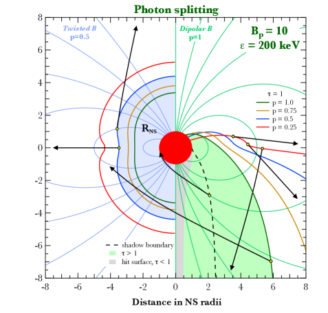
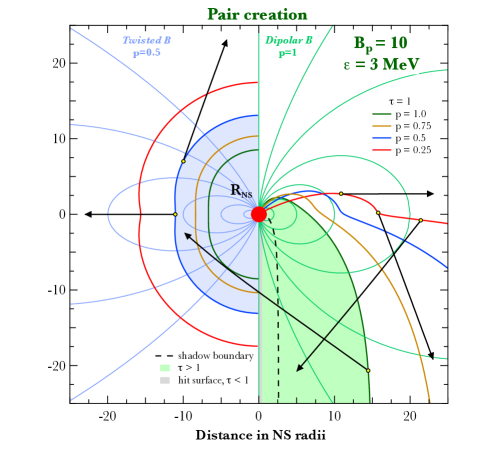
Figure 9: Sections of opaque volumes of polarization-averaged photon splitting (left panel) and pair creation (right panel) for photons with energy equal to 200 keV and 3 MeV, respectively. Photons are emitted in twisted magnetospheres in the Schwarzschild metric with $\,M=1.44M_{\odot}\,$ and $\,R_{\hbox{\sixrm NS}}=10^{6}\,$ cm. In each panel, colored contours are plotted for photons emitted outward and perpendicular to local field directions (left half) or parallel to the field directions inside the meridional plane (right half), with $\,p=0.25,0.5,0.75\,$, and $\,1.0\,$, as labelled, and generally ordered from lower to higher altitudes. All photon trajectories lie inside a meridional plane containing the star’s center. Photons emitted inside the contours are attenuated by photon splitting (left) or pair conversion (right). The shaded regions represent the opaque volumes for the outward emission with $\,p=0.5\,$ (blue) and for the parallel emission with $\,p=1\,$ (green), respectively. Photons emitted in these regions will be attenuated ($\,\tau>1\,$) before propagating to infinity or hitting the stellar surface. The dashed black curves define the boundaries of the shadow regions where emitted photons are on trajectories that will hit the surface; photons emitted in the gray interior shaded regions will hit the surface before being attenuated ($\,\tau<1\,$). Black curves with arrows signify photon paths for selected emission locales on different contours. Displayed magnetic field lines are projections onto the meridional plane; they are plotted in light blue (left, $\,p=0.5\,$) and light green (right, $\,p=1\,$; dipole).

The right panel in Fig. 9 presents the opaque volumes to photons with observed energy $\,\varepsilon=3\,$ MeV caused by polarization-averaged pair creation. The shapes of the contours are very similar to their photon splitting analogs on the left, yet the scales are larger due to the higher photon energy required to exceed the pair threshold, something that is also apparent in Figs. 3 and 5. As on the left, the transparent volume proximate to the north pole is enlarged as the twist increases, implying reduced rates of pair creation at altitudes $\,\mathrel{\mathchoice{\lower 2.0pt\vbox{\halign{$\m@th\displaystyle\hfil#\hfil$\cr<\crcr\sim\crcr}}}{\lower 2.0pt\vbox{\halign{$\m@th\textstyle\hfil#\hfil$\cr<\crcr\sim\crcr}}}{\lower 2.0pt\vbox{\halign{$\m@th\scriptstyle\hfil#\hfil$\cr<\crcr\sim\crcr}}}{\lower 2.0pt\vbox{\halign{$\m@th\scriptscriptstyle\hfil#\hfil$\cr<\crcr\sim\crcr}}}}8R_{\hbox{\sixrm NS}}\,$. The green and blue shaded areas, bounded by the dashed black curves, represent the opaque regions where emitted photons will be attenuated by splitting or pair conversion before propagating to infinity or striking the surface. The gray shaded area displays the interior shadow region where emitted photons actually reach the surface without attenuation ($\,\tau<1\,$). While not explicitly depicted, we remark that for photons of fixed energy $\,\varepsilon>2m_{e}c^{2}\,$ emitted parallel to $\,\bm{B}\,$ within the meridional plane, the opaque volumes of pair creation are larger than the photon splitting ones when the emission colatitude is not too small, $\,\theta_{\hbox{\fiverm E}}\mathrel{\mathchoice{\lower 2.0pt\vbox{\halign{$\m@th\displaystyle\hfil#\hfil$\cr>\crcr\sim\crcr}}}{\lower 2.0pt\vbox{\halign{$\m@th\textstyle\hfil#\hfil$\cr>\crcr\sim\crcr}}}{\lower 2.0pt\vbox{\halign{$\m@th\scriptstyle\hfil#\hfil$\cr>\crcr\sim\crcr}}}{\lower 2.0pt\vbox{\halign{$\m@th\scriptscriptstyle\hfil#\hfil$\cr>\crcr\sim\crcr}}}}60^{\circ}\,$.

The results displayed are for a choice of $\,B_{p}=10\,$. When the polar magnetic field is increased to $\,B_{p}=100\,$, the opacity volumes for both splitting and pair creation increase somewhat, as expected: a rise in the field strength throughout the magnetosphere increases the rates for both processes at each locale.

5.2 Discussion

The suite of results presented so far evinces two clear trends. First, there is a general increase of the opacity volumes in the inner magnetosphere when the twist is increased. This coupling is driven by the rise in the magnitude of the field, though a notable exception is in non-equatorial zones for outward emission parallel to $\,\bm{B}\,$. The second key trend is an increase of the escape energies with larger twists in the case of emission parallel to $\,\bm{B}\,$ on specified field loops somewhat near the poles. This behavior is caused by a general straightening of field lines, which then yields predominantly higher altitudes with lower fields where opaque conditions arise. While these trends may seem somewhat contradictory, they are actually encapsulated in the crossing over of opacity boundaries with different $\,p\,$ values in the upper hemispheres of the panels in Fig. 9. Addressing the impact of twists specifically on pair creation is also germane, since pair populations are believed to underpin the currents that establish the twisted fields on extended ranges of altitudes in the magnetosphere.

The commentary on Figure 8 in Section 4.3 focused on the gamma-ray transparency for magnetar giant flares. Also apparent in this polar zone figure is that $\,\varepsilon_{\rm esc}\,$ for the onset of pair creation domination of photon splitting increases modestly as the field twist rises, when the emission is parallel to $\,\bm{B}\,$. Yet, these pair onset $\,\varepsilon_{\rm esc}\,$ values do not change appreciably with variations in the twist parameter $\,p\,$ for emission orthogonal to the field. This reasonably implies that once sufficient pair creation is established to support significant twists, the configuration can sustain the twist as long as the energy source for a giant flare continues; the twist does not unduly starve itself of pairs. The pair conversion appears likely to occur at altitudes of 20-30 stellar radii, tapping the giant flare radiation supply there, only to cease at somewhat higher altitudes when the flare plasma outflow (likely ultra-relativistic: see Roberts et al., 2021) becomes optically thin to splitting and $\,\gamma\to e^{\pm}\,$ (yet still Thomson optically thick) and the radiation we see emerges.

The situation for persistent magnetospheric signals from magnetars may be quite different. Earlier figures such as Fig. 5 and 7 concentrate on larger footpoint colatitudes that are more or less commensurate with the active twist ones in the plasma simulations of Chen & Beloborodov (2017). For these field lines, the photon energies for the onset of pair creation in quasi-equatorial regions are only moderately increased by a strengthening of the twist. These field zones likely address the persistent hard X-ray tail emission (Thomson optically thin) of magnetars, which is known to not extend up to pair threshold (e.g., Kuiper et al., 2006; den Hartog et al., 2008a, b). Specifically, photons are easily generated to energies well in excess of 1 MeV in resonant inverse Compton models (Wadiasingh et al., 2018), tapping the energies of ultrarelativistic pairs accelerated in the magnetosphere. We anticipate that photon splitting strongly attenuates these gamma-rays (Wadiasingh et al., 2019), more so at higher fields and for higher twists, and may effectively starve the radiating plasma of pairs; this implies a possible limit to the maximal twist for normal magnetar activity.

Our results therefore highlight the need for a comprehensive inclusion of photon splitting opacity and its impact on pair creation inhibition in order to enhance simulations of dynamic, twisted magnetar magnetospheres, such as those studied in the works of Beloborodov (2009); Parfrey et al. (2013); Chen & Beloborodov (2017). It also identifies the compelling need for greater observational sensitivity in the 500 keV - 10 MeV band to afford more incisive probes of the shape of magnetar soft $\gamma$-ray spectra (Wadiasingh et al., 2019). This prospect could be fulfilled by a future Compton telescope such as NASA’s COSI SMEX mission, under development, and AMEGO or its more compact AMEGO-X version (Fleischhack et al., 2022).

5.2.1 Force-free MHD and Pulsar context for Twists

The employment of axi-symmetric force-free twists in this paper is a choice of simplicity and convenience. Force-free magnetosphere solutions for a rotating magnetic dipole field have been studied as models for rotation-powered pulsar magnetospheres over the last two decades. Solutions for both aligned (Contopoulos et al., 1999) and oblique (Spitkovsky, 2006) rotators have shown that the required current varies over the polar caps, ranging from super-Goldreich-Julian values, $J>J_{\rm GJ}=\rho_{\rm GJ}\,c$ where $\rho_{\rm GJ}=\Omega B/(2\pi c)$ is the Goldreich-Julian charge density (Goldreich & Julian, 1969) at the neutron star surface, to anti-Goldreich-Julian values, $J<0$. The charges to support the force-free magnetosphere are supplied by electron-positron production (above any electron-ion contribution), primarily in pair cascades near the polar caps. In order to supply the current in each part of the polar cap that is compatible with the force-free global current, these pair cascades must be non-stationary (Timokhin, 2010; Timokhin & Arons, 2013), producing bursts of pairs followed by screening of the electric field. So evidently, the magnetosphere cannot be force-free everywhere since pair production in pulsars requires particle acceleration.

The pair cascades are very localized in a small region near the polar caps since the microphysical processes involved in pair production operate on scales smaller than a neutron star radius. The length over which particles are accelerated combined with the photon mean-free path (essentially encapsulated in our calculations here) to produce a pair determines the location of the pair formation front and the size of the gap where force-free conditions are violated. Beyond the gap, force-free conditions can be established if the cascade can supply the global current. If all or parts of the magnetosphere become twisted (non-dipolar), there will be a different global current configuration with a bigger twist requiring a larger current (e.g. Beloborodov, 2009; Thompson, Lyutikov & Kulkarni, 2002). Therefore, any realistic, persistent magnetic twist must be in equilibrium with an adequate supply of pairs to supply the current for the force-free assumption, and the force-free conditions cannot co-exist with the regions of particle acceleration that are supplying the pairs and the currents. And since, as we have seen from dipolar pulsar magnetospheres, the currents are not likely to be spatially uniform, the twists are not likely to be axisymmetric as we have assumed. Our adoption of a force-free, axisymmetric twist is therefore idealized, and assumes that the current generated by the twist can be supplied by the pair plasma. As we have shown, an increasing twist decreases the opacity for pair production which may ultimately limit the amount of static force-free twist that is sustainable with a decreasing supply of pair plasma. Alternatively, a non-force-free (dissipative) twist configuration may be found that is consistent with the available pair plasma supply.

In a dynamical situation such as a magnetar burst, giant flare or enhanced persistent emission state (outburst), a sudden increase in twist may prevent the generation of enough pair plasma to supply the current (see the discussion above). In this case, the size of a force-free twist will decrease until the current it requires is consistent with what the pair plasma can supply. Depending on the charge supply, this may occur before the twist is large enough to form a resistive current sheet and undergo large-scale reconnection (Parfrey et al., 2013). Accordingly, it is apparent that the intricate interplay between twist morphology, pair creation and other sources of radiation opacity (principally photon splitting) is an essential ingredient of next-generation modeling of force-free or dissipative magnetar magnetospheres.

5.2.2 Magnetar Radio Emission Connections

This intimate interplay between field morphology and pair creation and photon splitting opacity is likely central to controlling the intensity and characteristics of persistent and transient radio emission from magnetars. The pair creation and cascading that precipitates such signals is thought to be initiated by curvature radiation gamma rays in pulsars, emission that emanates from polar field zones and is aligned closely to the local field direction $\,\hat{\bm{B}}\,$. The two panels in Fig. 8 highlight the extreme sensitivity of the escape energy to the axi-symmetric twist parameter $\,p\,$, with a dependence on the field footpoint colatitude $\,\theta_{\hbox{\sixrm f}}\,$ as the 6th power for the untwisted $\,p=1\,$ dipole, and even larger for twisted solutions; see Eq. (18). In more realistic magnetosphere constructions (i.e., more localized twists and non-ideal MHD conditions), plasma asymmetries that couple to the stellar rotation can have an impact in spite of magnetars being slow rotators with small polar caps and low Goldreich-Julian charge densities. The vector vorticity of the twist relative to the rotation vector $\,\bm{\hat{\Omega}}\,$ influences the polar field curvature considerably. Associated differences in the radius of field curvature will be reflected in the curvature emission photon energy, which along with the field morphology leads to a strong sensitivity of pair creation opacity to polar field geometry.

Thus small changes in the local field and accompanying modifications to the locale and shape of the pair formation front across the polar cap should have a dramatic impact on pulsed radio emission, its efficiency and spectrum, and also the beam morphology. Sensitive observations that exhibit dramatic changes in radio signals (e.g. Lower et al., 2021, for Swift J1818) suggest that even relatively quiescent X-ray magnetars possess dynamic magnetospheres near their polar caps.

For more energetic transient radio emission, i.e., FRBs, charge starvation at low altitudes near polar caps is also salient. Recently, Li et al. (2022) reported a $\sim 35-40$ Hz quasi-periodic oscillation in the X-ray burst (FRB-X) associated with the FRB-like radio bursts in SGR 1935+2154; this period matches well the temporal separation of the two radio burst peaks. Such a frequency is compatible with crustal torsional eigenmodes of neutron stars, conforming to predictions of “low-twist” magnetar FRB models of Wadiasingh & Timokhin (2019); Wadiasingh et al. (2020) that invoke crustal disturbances. Younes et al. (2021) argued that the FRB-X burst of SGR 1935+2154 is of quasi-polar origin due to its unusual spectral extension.

Burst-associated plasma waves set off by the crustal disturbances can trigger low-altitude pair cascades that can generate coherent plasma oscillations and radio emission. In such situations, Wadiasingh et al. (2020) showed that curvature radiation photons regulate pair formation and gaps (of voltages of the order of a TeV) in magnetars, and that splitting likely would not quench the pair cascades. Large persistent twists drive up pair opacity escape energies (see Fig. 8), and likely precipitate lower frequency curvature emission in the straighter field lines, thereby markedly reducing pair yields if the curvature photon energy is close to or below the pair escape energy. Accordingly, lower twists that permit modest pair creation at low altitudes are generally preferred conditions for FRB production in magnetars.

6 Conclusion

In this paper, photon opacities for the processes of photon splitting and pair creation are calculated in the twisted magnetospheres of magnetars. Fixing the polar field strength, axisymmetric MHD twisted magnetic fields embedded in the Schwarzschild metric were treated, for a variety of radial field scaling parameters $\,p\,$ (or equivalently, the maximal twist angle $\,\Delta\phi_{\rm tw}\,$). Given these assumptions, adding twists to the magnetic fields introduces toroidal field components, enhances the overall $\,|\bm{B}|\,$, and straightens the poloidal field lines. The twists also stretch magnetic field loops to higher altitudes due to the straightening of the field lines.

The impact of twists on photon opacity and escape energies $\,\varepsilon_{\rm esc}\,$ depends on the competition between field line straightening (decreases opacity) and field magnitude enhancement (increases opacity). Section 4 presented escape energies $\,\varepsilon_{\rm esc}\,$ for photons emitted from specified field loops. For photons that are emitted parallel to $\,\bm{B}\,$, the escape energy $\,\varepsilon_{\rm esc}\,$ rises with an increase of the twist (lower $\,p\,$), due to the straightening of the field lines if photons originate near the field loop footpoint, or lower fields encountered for emission nearer the equatorial apex of the loop. The opaque volume for magnetospheric emission generally increases for larger twists (see Fig. 9), mostly because of the increase of the field magnitude. An exception to this arises when photons are emitted parallel to the field lines in the polar regions, where field line straightening overrides the impact of the enhancement of the field magnitude.

In Section 4.3, which focused on photon opacity in the polar regions, the escape energy $\,\varepsilon_{\rm esc}\,$ of photons emitted parallel to $\,\bm{B}\,$ increases for larger twists and smaller footpoint colatitudes for the emission zones. Moreover, adding twists generally increases the pair creation opacity volume for photons with energies above the absolute pair threshold. Inside this opacity volume, pair creation prevails over photon splitting and dominates photon attenuation. Again, an exception occurs when photons are emitted parallel to $\,\bm{B}\,$ in the polar region, in which case the straightening of the field lines suppresses the development of $\,\varepsilon\sin\Theta_{\hbox{\sixrm kB}}\,$ during photon propagation. For photons emitted below pair threshold, the opaque volumes (now due to photon splitting) also increase.

The change of photon opacities due to the inclusion of twists has the potential to significantly modify the spectral characters of both persistent hard X-ray emission and magnetar giant flares. Our calculation provides a diagnostic tool to constrain the emission geometry of both signals, pertinent to data from missions such as Fermi-GBM, and could also be leveraged by future telescopes in the MeV band such as COSI and AMEGO.

ACKNOWLEDGMENTS

$${\cal F}^{\rm pp}_{\parallel}\;=\;\hbox{${{\displaystyle 2\vphantom{(}}\over{\displaystyle\varepsilon_{\perp}^{2}|p_{\hbox{\sevenrm 00}}|\vphantom{(}}}$}\,\exp\left(-\hbox{${{\displaystyle\varepsilon_{\perp}^{2}\vphantom{(}}\over{\displaystyle 2B\vphantom{(}}}$}\right) \quad,\quad 2<\varepsilon_{\perp}<1+\sqrt{1+2B}\quad,$$

$${\cal F}^{\rm pp}_{\perp}\;=\;\hbox{${{\displaystyle 2E_{0}(E_{0}+E_{1})\vphantom{(}}\over{\displaystyle\varepsilon_{\perp}^{2}|p_{\hbox{\sevenrm 01}}|\vphantom{(}}}$}\,\exp\left(-\hbox{${{\displaystyle\varepsilon_{\perp}^{2}\vphantom{(}}\over{\displaystyle 2B\vphantom{(}}}$}\right) \quad,\quad 1+\sqrt{1+2B}<\varepsilon_{\perp}<1+\sqrt{1+4B}\quad.$$

For these results, in the $\,\parallel\,$ case, the pairs are generated in only the ground state, whereas for the $\,\perp\,$ mode, the first excited state is sampled for one member of the electron-positron pair. In these expressions, the energies $\,E_{n}\,$ of the produced leptons and the corresponding momentum components $\,p_{jk}\,$ parallel to the magnetic field are

$$E_{0}=(1+p_{01}^{2})^{1/2}\quad,\quad E_{1}=(1+p_{01}^{2}+2B)^{1/2}\quad,\quad|p_{jk}|=\left[\hbox{${{\displaystyle\varepsilon_{\perp}^{2}\vphantom{(}}\over{\displaystyle 4\vphantom{(}}}$}-1-(j+k)B+\left(\hbox{${{\displaystyle(j-k)B\vphantom{(}}\over{\displaystyle\varepsilon_{\perp}\vphantom{(}}}$}\right)^{2}\right]^{1/2}\quad.$$ (22)

For energies above the lowest Landau levels, it is inefficient to use exact expressions that sum over many terms, so we then use the asymptotic expressions presented by Baier & Katkov (2007) that average over the many resonances. These forms are

$${\cal F}_{\parallel}\left(\varepsilon_{\perp},\,B\right)\;=\;\hbox{${{\displaystyle 1\vphantom{(}}\over{\displaystyle\sqrt{{\cal L}(\varepsilon_{\perp})\,\phi(\varepsilon_{\perp})}\vphantom{(}}}$}\,\exp\left\{-\hbox{${{\displaystyle\phi(\varepsilon_{\perp})\vphantom{(}}\over{\displaystyle 2B\vphantom{(}}}$}\right\}\quad,\quad{\cal F}_{\perp}\left(\varepsilon_{\perp},\,B\right)\;=\;\hbox{${{\displaystyle\varepsilon_{\perp}^{2}-4\vphantom{(}}\over{\displaystyle 2\varepsilon_{\perp}^{2}\vphantom{(}}}$}\,{\cal F}_{\parallel}\left(\varepsilon_{\perp},\,B\right)\quad,$$ (23)

where $\,\phi(\varepsilon_{\perp})\;=\;2\varepsilon_{\perp}-{\cal L}(\varepsilon_{\perp})\,$ and

$${\cal L}(\varepsilon_{\perp})\;=\;\hbox{${{\displaystyle\varepsilon_{\perp}^{2}-4\vphantom{(}}\over{\displaystyle 2\vphantom{(}}}$}\,\log_{e}\left(\hbox{${{\displaystyle\varepsilon_{\perp}+2\vphantom{(}}\over{\displaystyle\varepsilon_{\perp}-2\vphantom{(}}}$}\right)\quad.$$ (24)

Observe that all the $\,{\cal F}_{\perp,\parallel}\,$ functions are invariant under Lorentz transformations along B, for which $\,\varepsilon_{\perp}\,$ is constant.

Appendix B: Analytic Approximation of Escape Energy at Polar Regions

This Appendix details the derivation of the power law analytic approximation to the pair creation escape energy that is illustrated in the left panel of Fig. 8, and serves as a check on the numerical solutions in the quasi-polar domain. Given that it is applicable to high magnetospheric altitudes, GR modifications can be ignored. In the polar region, the flat-spacetime field structure in Eq. (9) can be well approximated by a first-order series expansion in small $\,\theta\,$, namely

$$\bm{B}\;\approx\;\frac{B_{p}}{r^{p+2}}\left(1,\;\frac{p}{2}\theta,\;\frac{1}{2}\sqrt{\frac{Cp}{p+1}}\theta^{1+2/p}\right)\quad,\quad\theta\;\ll\;1\quad.$$ (25)

Here $\,B_{p}\,$ is the surface field strength at the magnetic poles, $\,\theta\,$ is the magnetic colatitude, and $\,C=C(p)<1\,$ is the twist constant in Eq. (10). The toroidal field component $\,B_{\phi}\,$ can be neglected for small $\,\theta\,$ since it is much smaller than the poloidal components. Then the equation of a field line anchored near the magnetic pole at $\,\theta_{\hbox{\sixrm f}}\,$ can be obtained by integrating $\,dr/d\theta\,$ in Eq. (16) in flat spacetime; this yields

$$h\;=\;r/R_{\hbox{\sixrm NS}}\;\approx\;(\theta/\theta_{\hbox{\sixrm f}})^{2/p}\quad.$$ (26)

The trajectory of a photon emitted parallel to the local field direction lies essentially in the $\,(r,\theta)\,$ plane, a significant simplification for the purpose of opacity computations. In Section 3.1 of Story & Baring (2014), the optical depth for the photon emitted near the magnetic axis in a dipole field was analytically evaluated by integrating the attenuation coefficient in the meridional $\,(r,\theta)\,$ plane:

$$\tau(s)\;=\;\frac{\alpha_{\hbox{\sevenrm f}}}{\lambda\hbox to0.0pt{\hss--}_{c}}\int^{\eta(l)}_{0}B\sin{\Theta_{\hbox{\sixrm kB}}}\;{\cal F}(\omega_{\perp},B)\frac{ds}{d\eta}d\eta.$$ (27)

Here $\,s\,$ is the pathlength along the flat spacetime straight-line trajectory, and $\,\eta\,$ is the angle between $\,\bm{r}_{\hbox{\fiverm E}}\,$, the position vector of the emission locale, and $\,\bm{r}\,$, the position vector of the photon along its path (see Fig. 1 of Story & Baring, 2014). The optical depth in twisted field configurations can be obtained using the same method, with Eqs. (10) and (15) of Story & Baring (2014) being replaced by

$${\delta_{\hbox{\fiverm E}}}\;\approx\;\frac{p}{2}{\theta_{\hbox{\fiverm E}}}\quad,\quad B\;\approx\;\frac{B_{p}(\delta_{\hbox{\fiverm E}}-\eta)^{p+2}}{\delta_{\hbox{\fiverm E}}^{p+2}h^{p+2}}\quad\text{and}\quad\sin{\Theta_{\hbox{\sixrm kB}}}\approx\frac{p+2}{2}\eta\quad.$$ (28)

Here, $\,\delta_{\hbox{\fiverm E}}\,$ is the angle between the photon momentum $\,\mathbf{k}\,$, a constant during propagation, and the radial direction $\,\bm{r}_{\hbox{\fiverm E}}\,$ at the emission locale. Using the method of steepest descents to evaluate the optical depth integral in Eq. (1), analogous to the protocol adopted in Story & Baring (2014), the result is

$$\tau_{\rm Erber}\;\approx\;\frac{3^{2}p(p+2)^{3p/2+5/2}}{2^{8}(p+3)^{3p/2+4}}\left[\frac{p(2+p)\pi}{2}\frac{\varepsilon\theta_{\hbox{\sixrm f}}^{3}B_{p}^{3}}{h^{4+3p/2}}\right]^{1/2}\frac{\alpha_{\hbox{\sevenrm f}}R_{\hbox{\sixrm NS}}}{\lambdabar_{c}}\exp{\left[-\frac{2^{5}(p+3)^{p+3}}{3p(p+2)^{p+3}}\frac{h^{2+p/2}}{\varepsilon B_{p}\theta_{\hbox{\sixrm f}}}\right]}\quad.$$ (29)

The polarization-averaged pair creation rate presented in Eq. (3.3) of Erber (1966) was employed in developing this result, a rate that can be deduced by taking the $\,\varepsilon_{\perp}\gg 1\,$ limit of Eq. (23). The escape energy $\,\varepsilon\to\varepsilon_{\rm esc}\,$ can be then obtained by logarithmically inverting $\,\tau_{\rm Erber}=1\,$, yielding

$$\varepsilon_{\rm esc}\;\approx\;\frac{2^{5}(p+3)^{p+3}}{3p((p+2)^{p+3}}\frac{h^{2+p/2}}{B_{p}\theta_{\hbox{\sixrm f}}}\left\{\log{\left[\frac{3^{2}p(p+2)^{3p/2+5/2}}{2^{8}(p+3)^{3p/2+4}}\frac{\alpha_{\hbox{\sevenrm f}}R_{\hbox{\sixrm NS}}}{\lambdabar_{c}}\right]}+\frac{1}{2}\log{\left[\frac{p(2+p)\pi}{2}\frac{\varepsilon_{\rm esc}\theta_{\hbox{\sixrm f}}^{3}B_{p}^{3}}{h^{4+3p/2}}\right]}\right\}^{-1}\quad.$$ (30)

The second term in the curly brackets is much smaller than the first term for the range of altitudes, colatitudes and photon energies of relevance, so that neglecting it leads to Eq. (18), the result employed in the left panel of Fig. 8.

References

- Abdo et al. (2010) Abdo, A. A., Ackermann, M., Ajello, M., et al. 2010, ApJ, 725, L73. doi:10.1088/2041-8205/725/1/L73
- Adler (1971) Adler, S. L. 1971, Ann. Phys. 67, 599.
- Ajello et al. (2021) Ajello, M., Atwood, W. B., Axelsson, M., et al. 2021, Nat. Astron., 5, 385. doi:10.1038/s41550-020-01287-8
- Baier & Katkov (2007) Baier, V. N. & Katkov, V. M. 2007, Phys. Rev. D, 75, 073009 doi: 10.1103/PhysRevD.75.073009
- Baring (1995) Baring, M. G. 1995, ApJ, 440, L69. doi: 10.1086/187763
- Baring & Harding (1998) Baring, M. G. & Harding, A. K. 1998, ApJ, 507, L55. doi: 10.1086/311679
- Baring & Harding (2001) Baring, M. G. & Harding, A. K. 2001, ApJ, 547, 929. doi: 10.1086/318390
- Baring & Harding (2007) Baring, M. G. & Harding, A. K. 2007, Astrophys. Spac. Sci., 308, 109. doi: 10.1007/s10509-007-9326-x
- Baring et al. (2011) Baring, M. G., Wadiasingh, Z., & Gonthier, P. L. 2011, ApJ, 733, 61. doi: 10.1088/0004-637X/733/1/61
- ter Beek (2012) ter Beek, F. 2012, Masters thesis, University of Amsterdam.
- Beloborodov (2009) Beloborodov, A. M. 2009, ApJ, 703, 1044. doi: 10.1088/0004-637X/703/1/1044
- Beloborodov (2013) Beloborodov, A. M. 2013, ApJ, 762, 13. doi: 10.1088/0004-637X/762/1/13
- Bochenek et al. (2020) Bochenek, C. D., Ravi, V., Belov, K. V., et al. 2020, Nature, 587, 59. doi: 10.1038/s41586-020-2872-x
- Chen & Beloborodov (2017) Chen, A. Y., & Beloborodov, A. M. 2017, ApJ, 844, 133. doi: 10.3847/1538-4357/aa7a57
- Contopoulos et al. (1999) Contopoulos, I., Kazanas, D. & Fendt, C. 1999, ApJ, 511, 351. doi: 10.1086/306652
- Daugherty & Harding (1983) Daugherty, J. K. & Harding, A. K. 1983, ApJ, 273, 761. doi: 10.1086/161411
- Daugherty & Harding (1996) Daugherty, J. K. & Harding, A. K. 1996, ApJ, 458, 278. doi: 10.1086/176811
- Duncan & Thompson (1992) Duncan, R. C. & Thompson, C. 1992, ApJ, 392, L9. doi: 10.1086/186413
- Enoto et al. (2010) Enoto, T., Nakazawa, K., Makishima, K., et al. 2010, ApJ, 722, L162. doi:10.1088/2041-8205/722/2/L162
- Erber (1966) Erber, T. 1966, Rev. Mod. Phys., 38, 626. doi: 10.1103/RevModPhys.38.626
- Fernández & Thompson (2007) Fernández, R. & Thompson, C. 2007, ApJ, 660, 615. doi: 10.1086/511810
- Feroci et al. (2004) Feroci, M., Caliandro, G. A., Massaro, E., Mereghetti, S., & Woods, P. M. 2004, ApJ, 612, 408. doi: 10.1086/422405
- Fleischhack et al. (2022) Fleischhack, H. & Amego X Team 2021, 37th International Cosmic Ray Conference. 12-23 July 2021. Berlin, 649. arXiv:2108.02860
- Göǧüş et al. (1999) Göǧüş , E., Woods, P. M., Kouveliotou, C., et al. 1999, ApJ, 526, L93. doi: 10.1086/312380
- Goldreich & Julian (1969) Goldreich, P. & Julian, W. H. 1969, ApJ, 157, 869. doi: 10.1086/150119
- Gonthier et al. (2000) Gonthier, P. L., Harding A. K., Baring, M. G., et al. 2000, ApJ, 540, 907. doi:10.1086/309357
- Götz et al. (2006) Götz, D., Mereghetti, S., Tiengo, A. & Esposito, P. 2006, A&A, 449, L31. doi: 10.1051/0004-6361:20064870
- Grad & Rubin (1958) Grad, H. & Rubin, H. 1958, Proc. 2nd UN Conf. Peaceful Uses of Atomic Energy, 31, 190.
- Harding, Baring & Gonthier (1997) Harding, A. K., Baring, M. G. & Gonthier, P. L. 1997, ApJ, 476, 246. doi: 10.1086/303605
- Harding & Lai (2006) Harding, A. K. & Lai, D. 2006, Rep. Prog. Phys., 69, 2631 doi: 10.1088/0034-4885/69/9/R03
- den Hartog et al. (2008a) den Hartog, P. R., Kuiper, L., Hermsen, W., et al. 2008a, A&A, 489, 245. doi: 10.1051/0004-6361:200809390
- den Hartog et al. (2008b) den Hartog, P. R., Kuiper, L. & Hermsen, W. 2008b, A&A, 489, 263. doi:10.1051/0004-6361:200809772
- Heyl & Shaviv (2000) Heyl, J. S., & Shaviv, N. J. 2000, MNRAS, 311, 555, doi: 10.1046/j.1365-8711.2000.03076.x
- Hu et al. (2019) Hu, K., Baring, M. G., Wadiasingh, Z., et al. 2019, MNRAS, 486, 3327. doi:10.1093/mnras/stz995
- Hurley et al. (2005) Hurley, K., Boggs, S. E., Smith, D. M., et al. 2005, Nature, 434, 1098. doi: 10.1038/nature03519
- Hurley et al. (1999a) Hurley, K., Cline, T., Mazets, E., et al. 1999a, Nature, 397, 41. doi:10.1038/16199
- Hurley et al. (1999b) Hurley, K., Kouveliotou, C., Woods, P., et al. 1999b, ApJ, 510, L107. doi: 10.1086/311820
- Israel et al. (2008) Israel, G. L., Romano, P., Mangano, V., et al. 2008, ApJ, 685, 1114. doi: 10.1086/590486
- Kaspi & Beloborodov (2017) Kaspi, V. M. & Beloborodov, A. M. 2017, ARA&A, 55, 261. doi: 10.1146/annurev-astro-081915-023329
- Kojima (2017) Kojima Y., 2017, MNRAS, 468, 2011. doi:10.1093/mnras/stx584
- Kuiper et al. (2006) Kuiper, L., Hermsen, W., den Hartog, P. R. & Collmar, W. 2006, ApJ, 645, 556. doi: 10.1086/504317
- Li et al. (2022) Li, X., Ge, M., Lin, L., et al. 2022 ApJ, 931, 56. doi: 10.3847/1538-4357/ac6587
- Li et al. (2021) Li, C. K., Lin, L., Xiong, S. L., et al. 2021, Nat. Astron., 5, 378. doi:10.1038/s41550-021-01302-6
- Li et al. (2017) Li, J., Rea, N., Torres, D. F., et al. 2017, ApJ, 835, 30. doi:10.3847/1538-4357/835/1/30
- Lin et al. (2012) Lin, L., Göǧüş, E., Baring, M. G., et al. 2012, ApJ, 756, 54. doi: 10.1088/0004-637X/756/1/54
- Lin et al. (2011) Lin, L., Kouveliotou, C., Baring, M. G., et al. 2011, ApJ, 739, 87. doi: 10.1088/0004-637X/739/2/87
- Lower et al. (2021) Lower, M. E., Johnston, S., Shannon, R. M., Bailes, M., & Camilo, F. 2021, MNRAS, 502, 127. doi: 10.1093/mnras/staa3789
- Lüst & Schlüter (1954) Lüst R., Schlüter A., 1954, Z. Astrophys., 34, 263.
- Mazets et al. (1979) Mazets, E. P., Golenetskii, S. V., Il’Inskii, V. N., et al. 1979, Soviet Astronomy Lett., 5, 163
- Mereghetti et al. (2020) Mereghetti, S., Savchenko, V., Ferrigno, C., et al. 2020, ApJ, 898, L29. doi:10.3847/2041-8213/aba2cf
- Muslimov & Tsygan (1986) Muslimov, A. G. & Tsygan, A. I. 1986, Soviet Ast., 30, 567.
- Muslimov & Harding (2004) Muslimov, A. G. & Harding, A. K. 2004, ApJ, 606, 1143. doi: 10.1086/383079
- Olausen & Kaspi (2014) Olausen, S. A. & Kaspi, V. M. 2014, ApJS, 212, 6. doi: 10.1088/0067-0049/212/1/6
- Parfrey et al. (2013) Parfrey, K., Beloborodov, A. M. & Hui, L., 2013, ApJ, 774, 92. doi: 10.1088/0004-637X/774/2/92
- Pavan et al. (2009) Pavan L., Turolla R., Zane S., et al., 2009, MNRAS, 395, 753. doi: 10.1111/j.1365-2966.2009.14600.x
- Petterson (1974) Petterson, J. A. 1974, Phys. Rev. D, 10, 3166. doi:10.1103/PhysRevD.10.3166
- Poutanen (2020) Poutanen, J. 2020, A&A, 640, A24. doi: 10.1051/0004-6361/202037471
- Ridnaia et al. (2021) Ridnaia, A., Svinkin, D., Frederiks, D., et al. 2021, Nat. Astron., 5, 372. doi:10.1038/s41550-020-01265-0
- Roberts et al. (2021) Roberts, O. J., Veres, P., Baring, M. G., et al. 2021, Nature, 589, 207. doi:10.1038/s41586-020-03077-8
- Shafranov (1966) Shafranov, V. D. 1966, Reviews of Plasma Physics, 2, 103.
- Spitkovsky (2006) Spitkovsky, A. 2006, ApJ, 648, L51. doi: 10.1086/507518
- Story & Baring (2014) Story, S. A. & Baring, M. G. 2014, ApJ, 790, 61. doi: 10.1088/0004-637X/790/1/61
- Thompson & Duncan (1996) Thompson, C. & Duncan, R. C. 1996, ApJ, 473, 332. doi: 10.1086/178147
- Thompson, Lyutikov & Kulkarni (2002) Thompson, C., Lyutikov, M. & Kulkarni, S. R. 2002, ApJ, 574, 332. doi: 10.1086/340586
- Timokhin (2010) Timokhin, A. N. 2010, MNRAS, 408, 2092. doi: 10.1111/j.1365-2966.2010.17286.x
- Timokhin & Arons (2013) Timokhin, A. N.& Arons, J. 2013, MNRAS, 429, 20. doi: 10.1093/mnras/sts298
- Turolla et al. (2015) Turolla, R., Zane, S. & Watts, A. L. 2015, RPPh, 78, 116901. doi: 10.1088/0034-4885/78/11/116901
- van der Horst et al. (2012) van der Horst, A. J., Kouveliotou, C., Gorgone, N. M., et al. 2012, ApJ, 749, 122. doi: 10.1088/0004-637X/749/2/122
- Viganò (2013) Viganò, D., Rea, N., Pons, J. A., et al. 2013, MNRAS, 434, 123. doi: 10.1093/mnras/stt1008
- Wadiasingh et al. (2018) Wadiasingh, Z., Baring, M. G., Gonthier, P. L. & Harding, A. K. 2018, ApJ, 854, 98. doi: 10.3847/1538-4357/aaa460
- Wadiasingh et al. (2020) Wadiasingh, Z., Beniamini, P., Timokhin, A., et al. 2020, ApJ, 891, 82. doi: 10.3847/1538-4357/ab6d69
- Wadiasingh & Timokhin (2019) Wadiasingh, Z., & Timokhin, A. 2019, ApJ, 879, 4. doi: 10.3847/1538-4357/ab2240
- Wadiasingh et al. (2019) Wadiasingh, Z., Younes, G., Baring, M. G., et al 2019, arXiv:1903.05648
- Wasserman & Shapiro (1983) Wasserman I., Shapiro S. L., 1983, ApJ, 265, 1036. doi: 10.1086/160745
- Wolfson (1995) Wolfson R., 1995, ApJ, 443, 810. doi: 10.1086/175571
- Wolfson & Low (1992) Wolfson, R, & Low, B. C.., 1992, ApJ, 391, 353. doi: 10.1086/171350
- Woods et al. (1999) Woods, P. M., Kouveliotou, C., van Paradijs, J., et al. 1999, ApJ, 527, L47. doi:10.1086/312399
- Younes et al. (2017) Younes, G., Baring, M. G., Kouveliotou, C., et al. 2017, ApJ, 851, 17. doi: 10.3847/1538-4357/aa96fd
- Younes et al. (2021) Younes, G., Baring, M. G., Kouveliotou, C., et al. 2021, Nat. Astron., 5, 408. doi:10.1038/s41550-020-01292-x
- Younes et al. (2014) Younes, G., Kouveliotou, C., van der Horst, A. J., et al. 2014, ApJ, 785, 52. doi: 10.1088/0004-637X/785/1/52
- Younes et al. (2022) Younes, G., Lander, S. K., Baring, M. G., et al. 2022, ApJ, 924, L27. doi:10.3847/2041-8213/ac4700