Dynamical consistency conditions for
rapid turn inflation

Lilia Anguelova^a, Calin Iuliu Lazaroiu<sup>b

a</sup> Institute for Nuclear Research and Nuclear Energy,
Bulgarian Academy of Sciences, Sofia, Bulgaria
^b Horia Hulubei National Institute for Physics and Nuclear
Engineering (IFIN-HH), Bucharest-Magurele, Romania

Abstract

We derive consistency conditions for sustained slow roll and rapid turn inflation in two-field cosmological models with oriented scalar field space, which imply that inflationary models with field-space trajectories of this type are non-generic. In particular, we show that third order adiabatic slow roll, together with large and slowly varying turn rate, requires the scalar potential of the model to satisfy a certain nonlinear second order PDE, whose coefficients depend on the scalar field metric. We also derive consistency conditions for slow roll inflationary solutions in the so called “rapid turn attractor” approximation, as well as study the consistency conditions for circular rapid turn trajectories with slow roll in two-field models with rotationally invariant field space metric. Finally, we argue that the rapid turn regime tends to have a natural exit after a limited number of e-folds.

1 Introduction

Modern observations have established – to a very good degree of accuracy – that the present day universe is homogeneous and isotropic on large scales. This is naturally explained if one assumes that the early universe underwent a period of accelerated expansion called inflation. This idea can be realized in models where the inflationary expansion is driven by the potential energy of a number of real scalar fields called inflatons. The most studied models of this type contain a single scalar field. However, recent arguments related to quantum gravity suggest that it is more natural, or may even be necessary [1, 2, 3, 4] to have more than one inflaton. This has generated renewed interest in multi-field cosmological models, which had previously attracted only limited attention.

Multifield cosmological models have richer phenomenology than single field models since they allow for solutions of the equations of motion whose field-space trajectories are not (reparameterized) geodesics. Such trajectories are characterized by a non-zero turn rate. In the past it was thought that phenomenological viability requires small turn rate, by analogy with the slow roll approximation used in the single-field case. This assumption leads to the celebrated slow-roll slow-turn (SRST) approximation of [5, 6]. However, in recent years it was understood that rapid turn trajectories can also be (linearly) perturbatively stable [7, 8] and of phenomenological interest. For instance, a brief rapid turn during slow-roll inflation can induce primordial black hole generation [9, 10, 11, 12]; moreover, trajectories with large and constant turn rate can correspond to solutions behaving as dark energy [13, 14]. There is also a variety of proposals for full-fledged rapid-turn inflation models, relying on large turn rates during the entire inflationary period [15, 16, 20, 21, 18, 17, 19, 22].

Finding inflationary solutions in multifield models is much harder than in the single-field case, because the background field equations form a complicated coupled system of nonlinear ODEs. Thus usually such models are either studied numerically or solved only approximately. Mathematically, this complicated coupled system is encoded by the so-called cosmological equation, a nonlinear second order geometric ODE defined on the scalar field space of the model. The latter is a connected paracompact manifold, usually called the scalar manifold. In turn, the cosmological equation is equivalent with a dissipative geometric dynamical system defined on the tangent bundle of that manifold. Little is known in general about this dynamical system, in particular because the scalar manifold need not be simply-connected and – more importantly – because this manifold is non-compact in most applications of physical interest and hence cosmological trajectories can “escape to infinity”. The resulting dynamics can be surprisingly involved and hard to analyze even by numerical methods (see [28, 29, 30] for some nontrivial examples in two-field models), though a conceptual approach to some aspects of that dynamics was recently proposed in [31, 32].

A common approach to looking for cosmological trajectories with desirable properties is to first simplify the equations of motion by imposing various approximations (such as slow-roll to a certain order, rapid-turn and/or other conditions). This leads to an approximate system of equations, obtained by neglecting certain terms in the original ODEs. Then one attempts to solve the approximate system numerically or analytically. However, there is apriori no guarantee that a solution of the approximate system is a good approximant of a solution of the exact system for a sufficiently long period of time. In general, this will be the case only if the data which parameterizes the exact system (namely the scalar field metric and scalar potential of the model) satisfies appropriate consistency conditions. Despite being of fundamental conceptual importance, such consistency conditions have so far not been studied systematically in the literature.

In this paper, we investigate the problem of consistency conditions in two-field models with orientable scalar manifold for several commonly used approximations. First, we consider third order slow-roll trajectories with large but slowly varying turn rate. In this case, we show that compatibility with the equations of motion requires that the scalar potential satisfies a certain nonlinear second order PDE whose coefficients depend on the scalar field metric. This gives a nontrivial and previously unknown consistency condition that must be satisfied in the field-space regions where one can expect to find sustained rapid-turn trajectories allowing for slow roll inflation. Therefore, inflationary solutions of this type are not easy to find, implying that two-field models with such families of cosmological trajectories are non-generic. In particular, this shows that the difficulty in finding such models which was noticed in [33] is not related to supergravity, but arises on a more basic level.

We also discuss the case of rotationally invariant scalar field-space metrics. In that case, it is common to consider field space trajectories which are nearly circular as candidates for sustained rapid turn inflation. Imposing the first and second order slow roll conditions in this context leads to a certain consistency condition for compatibility with the equations of motion. This is again a PDE for the scalar potential with coefficients depending on the field space metric, which does not seem to have been widely noticed in the literature. We consider its implications for important examples in previous work.

Finally, we study in detail the consistency conditions for the approximation of [20], which subsumes many prominent rapid turn models of inflation. We show that this approximation is a special case of rapid turn with slow roll, instead of being equivalent to it. We then derive conditions for compatibility of this approximation with the equations of motion. Once again, these constrain the scalar potential and field space metric.

Throughout the paper, we assume that the field space (a.k.a. scalar manifold) of the two-field model is an oriented and connected paracompact surface. In our considerations, a crucial role is played by a fixed oriented frame (called the adapted frame) of vector fields defined on this surface which is determined by the scalar potential and field-space metric, instead of the moving oriented Frenet frame determined by the field space trajectory. The two frames are related to each other through a time-dependent rotation whose time-dependent angle we call the characteristic angle. We conclude our investigations by studying the time evolution of this angle. We show that, generically, this angle tends rather fast to the value $\pi\mod 2\pi$, which means that the tangent vector of the inflationary trajectory aligns with minus the gradient of the potential. This implies that the rapid turn regime has a natural exit in the generic case. Our results also suggest that it is difficult to sustain this regime for a prolonged period.

The paper is organized as follows. Section 2 recalls some basic facts about two-field cosmological models and introduces various parameters which will be used later on. Section 3 discusses the consistency condition for sustained rapid turn trajectories with third order slow roll, which results from careful analysis of the compatibility of the corresponding approximations with the equations of motion. Section 4 discusses the consistency condition for circular trajectories in rotationally-invariant models, as well as some implications for previous work on such inflationary trajectories. Section 5 discusses the approximation of [20], showing how it differs from rapid turn with second order slow roll and extracts the relevant consistency conditions. Section 6 studies the time evolution of the characteristic angle, while Section 7 presents our conclusions.

2 Two-field cosmological models

The action for $n$ real scalar fields $\varphi^{I}(x^{\mu})$ minimally coupled to four-dimensional gravity is:

$$S=\int d^{4}x\sqrt{-\det g}\left[\frac{R(g)}{2}-\frac{1}{2}G_{IJ}(\{\varphi^{I}\})\partial_{\mu}\varphi^{I}\partial^{\mu}\varphi^{J}-V(\{\varphi^{I}\})\right]\,\,\,,$$ (2.1)

where we took $M_{\mathrm{Pl}}=1$. Here $g_{\mu\nu}$ is the spacetime metric (which we take to have “mostly plus” signature) and $R(g)$ is its scalar curvature. The indices $\mu,\nu$ run from from $0$ to $3$ and $G_{IJ}$ is the metric on the scalar manifold (a.k.a. “scalar field space”) $\mathcal{M}$, which is parameterized by the scalars $\{\varphi^{I}\}$ with $I,J=1,...,n$. The scalar potential $V$ is a smooth real-valued function defined on $\mathcal{M}$, which for simplicity we take to be strictly positive. The standard cosmological Ansatze for the background metric and scalar fields are:

$$\mathrm{d}s^{2}_{g}=-\mathrm{d}t^{2}+a^{2}(t)\mathrm{d}\vec{x}^{2}\qquad,\qquad\varphi^{I}=\varphi^{I}(t)\quad,$$ (2.2)

where $a(t)>0$ is the scale factor. As usual, the definition of the Hubble parameter is:

$$H(t)=\frac{\dot{a}}{a}\,\,\,,$$ (2.3)

where the dot denotes derivation with respect to $t$.

With the Ansatze above, the equations of motion for the scalars reduce to:

$$D_{t}\dot{\varphi}^{I}+3H\dot{\varphi}^{I}+G^{IJ}V_{J}=0\quad,$$ (2.4)

where $V_{J}\stackrel{{\scriptstyle\mathrm{def.}}}{{=}}\partial_{J}V$ with $\partial_{J}\stackrel{{\scriptstyle\mathrm{def.}}}{{=}}\partial_{\varphi^{J}}$ and we defined:

$$D_{t}A^{I}\stackrel{{\scriptstyle\mathrm{def.}}}{{=}}\dot{\varphi}^{J}\,\nabla_{J}A^{I}=\dot{A}^{I}+\Gamma^{I}_{JK}(\varphi)\dot{\varphi}^{J}A^{K}$$

for any vector field $A^{I}$ defined on the scalar manifold, where $\Gamma^{I}_{JK}$ are the Christoffel symbols of $G_{IJ}$. The Einstein equations can be written as:

$$G_{IJ}\dot{\varphi}^{I}\dot{\varphi}^{J}=-2\dot{H}\qquad,\qquad 3H^{2}+\dot{H}=V\qquad.$$ (2.5)

In this paper we focus on two-field models, i.e. we take $n=2$. In this case, the scalar manifold $(\mathcal{M},{\cal G})$ is a (generally non-compact) Riemann surface, which we assume to be oriented. To define various characteristics of an inflationary solution, one introduces a frame of tangent vectors to the field space. A widely used choice is the positive Frenet frame, which consists of the tangent vector $T(t)$ and normal vector $N(t)$ to the trajectory $\varphi(t)=(\varphi^{1}(t),\varphi^{2}(t))\in\mathcal{M}$ of a solution of (2.4), where the normal vector is chosen such that $(T(t),N(t))$ forms a positively-oriented basis of the tangent space of the scalar manifold $\mathcal{M}$ at the point $\varphi(t)$. Let $\sigma$ be an increasing proper length parameter along the solution curve $\varphi$. This parameter is determined up to a constant translation and satisfies:

$$\dot{\sigma}=\sqrt{G_{IJ}\dot{\varphi}^{I}\dot{\varphi}^{J}}~{}~{}.$$

Then the vectors $T$ and $N$ are given by:

$$T^{I}=\frac{\mathrm{d}\varphi^{I}}{\mathrm{d}\sigma}=\frac{\dot{\varphi}^{I}}{\dot{\sigma}}$$

and

$$N_{I}=(\det G)^{1/2}\epsilon_{IJ}T^{J}\,\,\,.$$ (2.6)

One has:

$$N_{I}T^{I}=0\qquad,\qquad N_{I}N^{I}=1\qquad,\qquad T_{I}T^{I}=1\quad,$$ (2.7)

where $T_{I}=G_{IJ}T^{J}$ , $N^{I}=G^{IJ}N_{J}$ .

2.1 Characteristics of an inflationary solution

Consider the opposite relative acceleration vector:

$$\eta^{I}\stackrel{{\scriptstyle\mathrm{def.}}}{{=}}-\frac{1}{H\dot{\sigma}}D_{t}\dot{\varphi}^{I}\,\,\,.$$ (2.8)

Expanding $\eta$ in the orthonormal basis $(T,N)$ gives:

$$\eta^{I}=\eta_{\parallel}T^{I}+\eta_{\perp}N^{I}\,\,\,,$$

with:

$$\eta_{\parallel}=-\frac{\ddot{\sigma}}{H\dot{\sigma}}\qquad{\rm and}\qquad\eta_{\perp}=\frac{\Omega}{H}\,\,\,,$$ (2.9)

where we defined the signed turn rate of the trajectory $\varphi$ by:

$$\Omega\stackrel{{\scriptstyle\mathrm{def.}}}{{=}}-N_{I}D_{t}T^{I}\,\,\,.$$ (2.10)

The quantity $\eta_{\parallel}$ is called the second slow roll parameter of $\varphi$, while $\eta_{\perp}$ (which is sometimes denoted by $\omega$) is called the first turn parameter (or signed reduced turn rate). We will see in a moment that $\eta_{\parallel}$ is the second slow roll parameter of a certain one-field model determined by the trajectory $\varphi$. The second turn parameter is defined through:

$$\nu\stackrel{{\scriptstyle\mathrm{def.}}}{{=}}\frac{\dot{\eta}_{\perp}}{H\eta_{\perp}}~{}~{}.$$ (2.11)

It is a measure for the rate of change per e-fold of the dimensionless turn parameter $\eta_{\perp}$ .

Projecting the scalar field equations (2.4) along $T^{I}$ gives the adiabatic equation:

$$\ddot{\sigma}+3H\dot{\sigma}+V_{T}=0\,\,\,,$$ (2.12)

where $V_{T}\stackrel{{\scriptstyle\mathrm{def.}}}{{=}}T^{I}V_{I}$ . Projecting (2.4) along $N_{I}$  gives the entropic equation:

$$N_{I}D_{t}T^{I}=-\frac{V_{N}}{\dot{\sigma}}\,\,\,,$$ (2.13)

where $V_{N}\stackrel{{\scriptstyle\mathrm{def.}}}{{=}}N^{I}V_{I}$. Using the definition (2.10), the entropic equation (2.13) reads:

$$\Omega=\frac{V_{N}}{\dot{\sigma}}\,\,\,.$$ (2.14)

Let $V_{\varphi}(\sigma)\stackrel{{\scriptstyle\mathrm{def.}}}{{=}}V(\varphi(\sigma))$. Then:

$$V_{T}=\frac{\mathrm{d}V_{\varphi}}{\mathrm{d}\sigma}=V^{\prime}_{\varphi}(\sigma)~{}~{},$$

where the prime denotes derivation with respect to $\sigma$. Hence the adiabatic equation (2.12) reads:

$$\ddot{\sigma}+3H\dot{\sigma}+V_{\varphi}^{\prime}(\sigma)=0\,\,\,,$$

which shows that $\sigma$ obeys the equation of motion of a one-field model with scalar potential $V_{\varphi}$. Since for an expanding universe we have $H>0$ , the Hubble parameter can be expressed from (2.5) as:

$$H(\sigma,\dot{\sigma})=\frac{1}{\sqrt{6}}\sqrt{\dot{\sigma}^{2}+2V(\sigma)}~{}~{},$$

which is the usual formula for a single-field model.

The adiabatic Hubble slow roll parameters of the trajectory $\varphi$ are defined as the usual Hubble slow roll-parameters [34] of the adiabatic one-field model defined above. The first three of these are:

$$\varepsilon\stackrel{{\scriptstyle\mathrm{def.}}}{{=}}-\frac{\dot{H}}{H^{2}}\qquad,\qquad\eta_{\parallel}=-\frac{\ddot{\sigma}}{H\dot{\sigma}}\qquad,\qquad\xi\stackrel{{\scriptstyle\mathrm{def.}}}{{=}}\frac{\dddot{\sigma}}{H^{2}\dot{\sigma}}~{}~{},$$ (2.15)

where for $\xi$ we use a different sign convention than [34]. Since all results of [34] apply to the adiabatic one field models, it follows that the following relations hold on-shell:

$$\epsilon_{T}=\varepsilon\left(\frac{3-\eta_{\parallel}}{3-\varepsilon}\right)^{2}$$

$$\eta_{\parallel}=\varepsilon-\frac{\varepsilon^{\prime}}{\sqrt{2\varepsilon}}$$

$$\eta_{T}=\sqrt{2\varepsilon}\frac{\eta^{\prime}_{\parallel}}{3-\varepsilon}+\frac{3-\eta_{\parallel}}{3-\varepsilon}(\varepsilon+\eta_{\parallel})~{}~{},$$

where the adiabatic first and second potential slow roll parameters are defined through:

$$\epsilon_{T}\stackrel{{\scriptstyle\mathrm{def.}}}{{=}}\frac{1}{2}\left(\frac{V_{T}}{V}\right)^{2}~{}~{},~{}~{}\eta_{T}\stackrel{{\scriptstyle\mathrm{def.}}}{{=}}\frac{V^{\prime\prime}_{\varphi}}{V}~{}~{}.$$

2.2 Slow roll and rapid turn regimes

The first, second and third slow roll regimes are defined respectively by the conditions $\varepsilon\ll 1$, $|\eta_{\parallel}|\ll 1$ and $|\xi|\ll 1$. The second order slow roll regime is defined by the two conditions $\varepsilon\ll 1$ and $|\eta_{\parallel}|\ll 1$ taken together, while the third order slow roll regime is defined by the three conditions $\varepsilon\ll 1$, $|\eta_{\parallel}|\ll 1$ and $|\xi|\ll 1$ considered together.

The first order rapid turn regime is defined by the condition:

$$\eta_{\perp}^{2}\gg 1\,\,\,,$$ (2.16)

while the condition $|\nu|\ll 1$ defines the second order rapid turn regime. A trajectory has sustained rapid turn if both of the conditions $\eta_{\perp}^{2}\ll 1$ and $|\nu|\ll 1$ are satisfied.

In the first slow roll regime $\varepsilon\ll 1$, the second equation in (2.5) becomes:

$$3H^{2}\approx V\,\,\,.$$ (2.17)

Together with (2.14), this gives:

$$\eta_{\perp}^{2}=\frac{\Omega^{2}}{H^{2}}\approx\frac{3V_{N}^{2}}{\dot{\sigma}^{2}V}\,\,\,.$$ (2.18)

2.3 Some other useful parameters

For our purpose, it will be useful to consider two other parameters, which are related to the familiar ones reviewed above. The first IR parameter is the ratio of the kinetic and potential energies of the scalars:

$$\kappa\stackrel{{\scriptstyle\mathrm{def.}}}{{=}}\frac{G_{IJ}\dot{\varphi}^{I}\dot{\varphi}^{J}}{2V}=\frac{\dot{\sigma}^{2}}{2V}\,\,\,.$$ (2.19)

This parameter plays an important role in the IR approximation discussed in [31] and [32]. On solutions of the equations of motion, the first slow roll parameter can be written as:

$$\varepsilon=\frac{3\dot{\sigma}^{2}}{\dot{\sigma}^{2}+2V}\,\,\,.$$

Hence the on-shell value of the first slow roll parameter is related to the first IR parameter through:

$$\varepsilon=\frac{3\kappa}{1+\kappa}\,\,\,.$$ (2.20)

This relation shows that the first slow roll condition $\varepsilon\ll 1$ is equivalent with $\kappa\ll 1$ , whereas $\varepsilon=1$ corresponds to $\kappa=\frac{1}{2}$ . In particular, the condition for inflation $\varepsilon<1$ is equivalent with $\kappa<\frac{1}{2}$.

We also define the conservative parameter:

$$c\stackrel{{\scriptstyle\mathrm{def.}}}{{=}}\frac{H\dot{\sigma}}{\sqrt{G^{IJ}V_{I}V_{J}}}\,\,\,,$$ (2.21)

which is small iff the friction term can be neglected relative to the gradient term in the equation of motion for the scalar fields. When $c\ll 1$, the motion of $\varphi$ is approximately conservative in the sense that the total energy $\frac{1}{2}G_{IJ}\dot{\varphi}^{I}\dot{\varphi}^{J}$ of the scalar fields is approximately conserved; in this limit, the equations of motion for the scalars reduce to:

$$\nabla_{t}\varphi^{I}+G^{IJ}\partial_{J}V\approx 0~{}~{},$$

which describe the motion of a particle in the Riemannian manifold $(\mathcal{M},{\cal G})$ under the influence of the potential $V$. We will see below that, in the second slow roll regime $|\eta_{\parallel}|\ll 1$, the rapid turn condition (2.16) is equivalent with the conservative condition:

$$c^{2}\ll 1\,\,\,.$$

3 The consistency condition for sustained slow roll with rapid turn

In this section, we derive a constraint relating the scalar potential $V$ and the field-space metric $G_{IJ}$  which is necessary for existence of rapid turn solutions ($\eta_{\perp}^{2}\gg 1$) that satisfy the third order slow roll conditions $\varepsilon\ll 1$, $|\eta_{\parallel}|\ll 1$ and $|\xi|\ll 1$  as well as the second order condition $|\nu|\ll 1$ for slowly-varying turn rate. The last condition is usually imposed to ensure the longevity of the rapid-turn slow-roll regime (so that it could produce about 50-60 e-folds of inflation). The constraint we derive does not require any extraneous assumptions about the potential, the field space metric or the shape of the field-space trajectory.

3.1 The adapted frame

We will use a globally-defined frame $(n,\tau)$ (which we call the adapted frame) of the scalar manifold determined by $V$ and $G_{IJ}$. Namely, we take $n$ to be the unit vector field along the gradient of the potential:

$$n\stackrel{{\scriptstyle\mathrm{def.}}}{{=}}\frac{\nabla V}{\sqrt{G^{IJ}V_{I}V_{J}}}\quad,\,\,{\rm with\,\,components}\quad n^{K}=\frac{G^{KL}V_{L}}{\sqrt{G^{IJ}V_{I}V_{J}}}\,\,\,.$$ (3.1)

The unit vector $\tau$ is orthogonal to $n$ and chosen such that the basis $(n,\tau)$ is positively oriented:

$$\tau_{I}=(\det G)^{1/2}\epsilon_{IJ}n^{J}\,\,\,.$$ (3.2)

We have $\tau^{I}\stackrel{{\scriptstyle\mathrm{def.}}}{{=}}G^{IJ}\tau_{J}$ as usual. The relation between the two bases is given by:

$$T = ~{}\,\cos\theta_{\varphi}\,\,n+\sin\theta_{\varphi}\,\,\tau\,\,\,,$$

$$N = -\!\sin\theta_{\varphi}\,\,n+\cos\theta_{\varphi}\,\,\tau\,\,\,,$$ (3.3)

where $\theta_{\varphi}\in(-\pi,\pi]$ is the characteristic angle of $\varphi$, which is defined as the angle of the rotation that takes the oriented basis $(n,\tau)$ to the oriented basis $(T,N)$ at the point of interest on the cosmological trajectory.

3.2 Expressing $\eta_{\parallel}$ and $\eta_{\perp}$ in terms of $\theta_{\varphi}$ and $c$

Relation (2.9) and the adiabatic equation (2.12) give:

$$\eta_{\parallel}=3+\frac{V_{\sigma}}{H\dot{\sigma}}=3+\frac{T^{I}G_{IJ}n^{J}}{H\dot{\sigma}}\sqrt{G^{KL}V_{K}V_{L}}=3+\frac{\cos\theta_{\varphi}}{c}\,\,\,,$$ (3.4)

where the conservative parameter $c$ was defined in (2.21). Notice that $\eta_{\parallel}\approx 3$ for either $\cos\theta_{\varphi}\approx 0$ or $c\gg 1$ . Also, the second slow roll condition $|\eta_{\parallel}|\ll 1$ requires that $c<1$ and $\cos\theta_{\varphi}<0$ . In fact, $\eta_{\parallel}\approx 0$ is achieved for $c\approx-\cos\theta_{\varphi}/3$ .

We next consider equation (2.9) for $\eta_{\perp}$. Using the entropic equation (2.14) and substituting $N$ from (3.1) gives:

$$\eta_{\perp}=\frac{\Omega}{H}=\frac{N_{I}V^{I}}{\dot{\sigma}H}=-\frac{(G^{KL}V_{K}V_{L})^{\frac{1}{2}}\sin\theta_{\varphi}}{\dot{\sigma}H}=-\frac{\sin\theta_{\varphi}}{c}\,\,\,.$$ (3.5)

In the second slow roll approximation we have  $c\approx-\cos\theta_{\varphi}/3$  (as explained above) and equation (3.5) gives:

$$\eta_{\perp}^{2}\approx 9\,\tan^{2}\theta_{\varphi}\,\,\,.$$ (3.6)

Hence the rapid turn condition $\eta_{\perp}^{2}\gg 1$ is equivalent with $\tan^{2}\theta_{\varphi}\gg 1$ or, equivalently, with $\cos^{2}\theta_{\varphi}\ll 1$ . In view of (3.4), it follows that the second slow roll condition $|\eta_{\parallel}|\ll 1$ requires $c^{2}\ll 1$ . Note that $c$ itself does not need to be very small. It is enough to have $c\sim{\cal O}(10^{-1})$ , in order to ensure rapid turn and slow roll.

The discussion above shows that the slow roll and rapid turn regime, which is usually defined by:

$$\varepsilon\ll 1\quad,\quad|\eta_{\parallel}|\ll 1\quad,\quad\eta_{\perp}^{2}\gg 1\,\,\,,$$ (3.7)

is characterized equivalently by:

$$\varepsilon\ll 1\quad,\quad|\eta_{\parallel}|\ll 1\quad,\quad c^{2}\ll 1\,\,\,.$$ (3.8)

We next derive the consistency condition on $V$ and $G_{IJ}$ in this regime, supplemented by the additional requirements that:

$$|\xi|\ll 1\quad{\rm and}\quad|\nu|\ll 1\,\,\,,$$ (3.9)

where $\xi$ is the third order slow roll parameter in (2.15), while $\nu$ is the relative rate of change of $\eta_{\perp}$ as defined in (2.11). The purpose of the second condition in (3.9) is to ensure that the inequality (2.16) is satisfied for a prolonged period. (Note that $|\nu|\ll 1$ does not follow from the slow roll conditions in (3.7).)

3.3 The condition for sustained rapid turn with third order slow roll

The equations of motion (2.12) and (2.14) respectively imply (see [35, 36, 37]):

$$\frac{V_{TT}}{3H^{2}} = \frac{\Omega^{2}}{3H^{2}}+\varepsilon+\eta_{\parallel}-\frac{\xi}{3}\,\,\,,$$

$$\frac{V_{TN}}{H^{2}} = \frac{\Omega}{H}\left(3-\varepsilon-2\eta_{\parallel}+\nu\right)\,\,\,.$$ (3.10)

We will study the consequences of these relations for inflation with third order slow roll, defined by:

$$\varepsilon\,,\,|\eta_{\parallel}|\,,\,|\xi|\ll 1\,\,\,,$$ (3.11)

while also imposing the condition:

$$|\nu|\ll 1\,\,\,.$$ (3.12)

The latter ensures a small rate of change of the large turn rate and hence longevity of the rapid turn regime.

In the regime defined by (3.11)-(3.12), equations (3.3) imply:

$$V_{TT}\approx\frac{1}{9}\frac{V_{TN}^{2}}{H^{2}}\,\,\,.$$ (3.13)

Recalling that $3H^{2}\approx V$ (see (2.17)), relation (3.13) can be written as:

$$V_{TT}\approx\frac{1}{3}\frac{V_{TN}^{2}}{V}\,\,\,.$$ (3.14)

To extract conditions on $V$ and $G_{IJ}$ , let us rewrite (3.14) in terms of $V_{nn}$, $V_{n\tau}$ and $V_{\tau\tau}$ . Using (3.1), we have:

$$V_{TT} = T^{I}T^{J}\nabla_{I}V_{J}=V_{nn}\cos^{2}\theta_{\varphi}+2V_{n\tau}\sin\theta_{\varphi}\cos\theta_{\varphi}+V_{\tau\tau}\sin^{2}\theta_{\varphi}\,\,\,,$$

$$V_{TN} = T^{I}N^{J}\nabla_{I}V_{J}=\left(V_{\tau\tau}-V_{nn}\right)\cos\theta_{\varphi}\sin\theta_{\varphi}+V_{n\tau}\left(\cos^{2}\theta_{\varphi}-\sin^{2}\theta_{\varphi}\right)\,\,.$$ (3.15)

With the approximations (3.8), one has  $\cos\theta_{\varphi}\approx-3c$  due to (3.4) . In that case $\sin\theta_{\varphi}\approx s\sqrt{1-9c^{2}}$ , where $s=\pm 1$ . Hence (3.3) becomes:

$$V_{TT} \approx 9c^{2}V_{nn}-6sc\,\sqrt{1-9c^{2}}\,V_{n\tau}+(1-9c^{2})V_{\tau\tau}\,\,\,,$$

$$V_{TN} \approx -3sc\,\sqrt{1-9c^{2}}\left(V_{\tau\tau}-V_{nn}\right)-(1-18c^{2})V_{n\tau}\,\,\,.$$ (3.16)

Since the different components of the Hessian of $V$ may be of different orders in the small parameter $c$ , we cannot conclude from (3.3) that $V_{TT}\approx V_{\tau\tau}$ and $V_{TN}\approx-V_{n\tau}$ . Instead, we need two relations between $V_{nn}$, $V_{n\tau}$, $V_{\tau\tau}$ and $c$ , in order to be able to solve for $c$ and then extract a relation, that involves only the components of the Hessian of $V$ .

To achieve this, let us compute (3.3) in terms of $c$ in the regime (3.8):

$$\frac{V_{TT}}{3H^{2}} \approx \frac{\Omega^{2}}{3H^{2}}=\frac{\sin^{2}\theta_{\varphi}}{3\,c^{2}}\approx\frac{1}{3\,c^{2}}-3\,\,\,,$$

$$\frac{V_{TN}}{H^{2}} \approx 3\frac{\Omega}{H}=-\frac{3\,\sin\theta_{\varphi}}{c}\approx-\frac{3s}{c}\sqrt{1-9c^{2}}\,\,\,,$$ (3.17)

where we used (3.5) together with  $\sin\theta_{\varphi}\approx s\sqrt{1-9c^{2}}$ . Since $3H^{2}\approx V$ during slow roll, we have:

$$V_{TT}\approx\frac{V}{3\,c^{2}}-3V\qquad{\rm and}\qquad V_{TN}\approx-\frac{s}{c}\sqrt{1-9c^{2}}\,V\quad.$$ (3.18)

These expressions satisfy (3.14) automatically, as should be the case. Now substitute (3.3) in (3.18). This gives the following two relations:

$$\frac{V}{3\,c^{2}}-3V \approx 9c^{2}V_{nn}-6sc\,\sqrt{1-9c^{2}}\,V_{n\tau}+(1-9c^{2})V_{\tau\tau}\,\,\,,$$

$$\frac{s}{c}\sqrt{1-9c^{2}}\,V \approx 3sc\,\sqrt{1-9c^{2}}\left(V_{\tau\tau}-V_{nn}\right)+(1-18c^{2})V_{n\tau}\,\,\,.$$ (3.19)

Our next goal is to eliminate the small parameter $c$  without making any assumptions about the order of any of the quantities $V$, $V_{nn}$, $V_{n\tau}$, $V_{\tau\tau}$. We begin by solving for $V_{n\tau}$ from the second equation in (3.3):

$$V_{n\tau}\,\approx\,\frac{s\sqrt{1-9c^{2}}}{(1-18c^{2})}\left[\frac{V}{c}-3c\left(V_{\tau\tau}-V_{nn}\right)\right]\,\,.$$ (3.20)

Substituting this in the first equation of (3.3) gives:

$$(1-18c^{2})\left(\frac{V}{3\,c^{2}}-3V\right)\approx-6V+54c^{2}V-9c^{2}V_{nn}+(1-9c^{2})V_{\tau\tau}\,\,\,,$$ (3.21)

where we did not drop any term containing higher powers of $c$ ; at intermediate steps there are terms with $c^{4}$ , as well as other $c^{2}$ terms, but they all cancel exactly. Since $(1-18c^{2})\left(\frac{V}{3\,c^{2}}-3V\right)=\frac{V}{3c^{2}}-3V-6V+54c^{2}V$  relation (3.21) becomes:

$$\frac{V}{3\,c^{2}}-3V\,\approx\,-9c^{2}V_{nn}+(1-9c^{2})V_{\tau\tau}\,\,\,.$$

Thus:

$$V_{\tau\tau}\,\approx\,\frac{\frac{V}{3\,c^{2}}-3V+9c^{2}V_{nn}}{1-9c^{2}}\,\,\,.$$ (3.22)

Note that this expression for $V_{\tau\tau}$ was obtained without neglecting any terms compared to (3.3). From (3.22), we have:

$$V_{\tau\tau}\approx\frac{V}{3c^{2}}+9c^{2}V_{nn}+{\cal O}(c^{4})\,\,\,.$$ (3.23)

Substituting (3.22) in (3.20), we find:

$$V_{n\tau}\approx\frac{3scV_{nn}}{\sqrt{1-9c^{2}}}\,\,\,,$$ (3.24)

where the terms with $V$ canceled exactly. We stress that the result (3.24) was obtained without neglecting any further terms, just like (3.22). Now recall that in the rapid turn regime we have $c^{2}\ll 1$ . Hence in this regime equations (3.22) and (3.24) imply:

$$V_{\tau\tau}\approx\frac{V}{3c^{2}}\qquad{\rm and}\qquad V_{n\tau}\approx 3scV_{nn}\,\,\,.$$ (3.25)

The second relation gives:

$$c\approx\frac{s}{3}\frac{V_{n\tau}}{V_{nn}}\,\,\,.$$ (3.26)

Substituting this into the first relation of (3.25) gives:

$$3VV_{nn}^{2}\approx V_{n\tau}^{2}V_{\tau\tau}\,\,\,.$$ (3.27)

Since $V>0$ , the last relation implies, in particular, that we have:

$$V_{\tau\tau}>0\,\,\,.$$ (3.28)

In view of (3.23), the Hessian of $V$ takes the following form to order $c^{2}$ :

$$\left[\begin{array}[]{cc}V_{\tau\tau}&~{}~{}V_{n\tau}\\ V_{n\tau}&~{}~{}V_{nn}\end{array}\right]\approx\left[\begin{array}[]{cc}9c^{2}V_{nn}+\frac{V}{3c^{2}}&~{}~{}~{}3scV_{nn}\\ 3scV_{nn}&~{}~{}~{}V_{nn}\end{array}\right]~{}~{}.$$

The eigenvalues of the characteristic polynomial of this matrix are:

$$\lambda_{1}\approx V_{nn}\qquad{\rm and}\qquad\lambda_{2}\approx\frac{V}{3\,c^{2}}\quad,$$

where we used $c^{2}\ll 1$ . Hence the Hessian of the potential has non-negative eigenvalues when:

$$V_{nn}\geq 0\,\,\,.$$

In view of (3.25), the second eigenvalue is given by $\lambda_{2}\approx V_{\tau\tau}$ . This is consistent with the fact that (3.26) implies (to leading order in the slow roll and rapid turn regime) that the Hessian of $V$ is diagonal in the basis $(n,\tau)$ .

From (3.27) we have:

$$V_{\tau\tau}\approx 3V\frac{V_{nn}^{2}}{V_{n\tau}^{2}}\,\,\,.$$ (3.29)

Let us compare this with the expression for $V_{\tau\tau}$ in (3.23). Substituting (3.26) in (3.23) gives:

$$V_{\tau\tau}\approx\frac{V}{3\,c^{2}}+9c^{2}V_{nn}\approx 3V\frac{V_{nn}^{2}}{V_{n\tau}^{2}}+\frac{V_{n\tau}^{2}}{V_{nn}}\,\,\,.$$ (3.30)

Using (3.29) and (3.30) we conclude that:

$$V_{\tau\tau}V_{nn}\gg V_{n\tau}^{2}\,\,\,.$$ (3.31)

Notice that the consistency condition (3.27) depends not only on $V$ but also on the field-space metric $G_{IJ}$ , as is clear from the definitions of the basis vectors $n$ and $\tau$ .

Finally, let us discuss the special case when $V_{n\tau}=0$ . In this case, we must reconsider (3.3), since (3.26) gives $c\approx 0$ . So let us take $V_{n\tau}=0$ in (3.3):

$$\frac{V}{3\,c^{2}}-3V \approx 9c^{2}V_{nn}+(1-9c^{2})V_{\tau\tau}\,\,\,,$$

$$\frac{s}{c}\sqrt{1-9c^{2}}\,V \approx 3sc\,\sqrt{1-9c^{2}}\left(V_{\tau\tau}-V_{nn}\right)\,\,\,.$$ (3.32)

The second relation gives:

$$V_{\tau\tau}\approx\frac{V}{3c^{2}}+V_{nn}\,\,\,.$$

Substituting this into the first equation in (3.3) we obtain:

$$V_{nn}\approx 0\,\,\,,$$ (3.33)

where we did not neglect any terms; everything except $V_{nn}$ canceled exactly. Thus, the consistency condition (3.27) is satisfied again, although relation (3.31) is not valid anymore.

To recapitulate the considerations of this Section: We have shown that (3.27) is a necessary condition for the existence of a prolonged inflationary period in the slow-roll and rapid-turn regime defined by (3.7) and (3.9). Note that, since $V_{nn}=n^{I}n^{J}\nabla_{I}V_{J}$ and similarly for $V_{n\tau}$ and $V_{\tau\tau}$ , equation (3.27) is a rather complicated PDE, whose coefficients depend on the scalar field-space metric $G_{IJ}$ . Hence, solving it systematically, for instance in order to determine the potential for a given metric (or vice versa), is a very complicated problem. We certainly hope to report on progress in that regard, for some classes of scalar field metrics, in the future.

4 The case of rotationally invariant metrics

In the literature on cosmological inflation the field-space metric $G_{IJ}$ is often assumed to be rotationally invariant. Partly, this is motivated by the desire for simplification. It is also the case that many inflationary models which arise from string theory compactifications have a scalar field metric of this type. In view of this, we will now specialize the consistency conditions derived in the previous Section to the case of rotationally invariant metrics.

For such metrics, the consistency condition extracted in the previous section can be made explicit upon using local semigeodesic coordinates on the scalar manifold $(\mathcal{M},{\cal G})$, in which the metric has the form:

$$\mathrm{d}s^{2}_{G}=\mathrm{d}r^{2}+h^{2}(r)\mathrm{d}\theta^{2}\,\,\,$$ (4.1)

with $h(r)>0$ . In such coordinates, the non-vanishing Christoffel symbols are:

$$\Gamma^{r}_{\theta\theta}=-hh^{\prime}\qquad,\qquad\Gamma^{\theta}_{r\theta}=\frac{h^{\prime}}{h}\quad,$$ (4.2)

where the prime denotes derivation with respect to $r$. Let us compute the components of the Hessian, which enter the condition (3.27). Using (3.1), (3.2) and (4.1), we obtain:

$$V_{nn} = n^{I}n^{J}\nabla_{I}\nabla_{J}V$$ (4.3)

$$= \frac{1}{(h^{2}V_{r}^{2}+V_{\theta}^{2})}\left[h^{2}V_{r}^{2}V_{rr}+2V_{r}V_{\theta}V_{r\theta}-\frac{h^{\prime}}{h}V_{r}V^{2}_{\theta}+\frac{1}{h^{2}}V_{\theta}^{2}V_{\theta\theta}\right]\,,$$

$$V_{n\tau} = n^{I}\tau^{J}\nabla_{I}\nabla_{J}V$$ (4.4)

$$= \frac{h}{(h^{2}V_{r}^{2}+V_{\theta}^{2})}\left[V_{r}V_{\theta}\left(V_{rr}-\frac{1}{h^{2}}V_{\theta\theta}\right)+\left(\frac{1}{h^{2}}V^{2}_{\theta}-V_{r}^{2}\right)V_{r\theta}-\frac{h^{\prime}}{h^{3}}V^{3}_{\theta}\right]\,,$$

$$V_{\tau\tau} = \tau^{I}\tau^{J}\nabla_{I}\nabla_{J}V$$ (4.5)

$$= \frac{h^{4}}{(h^{2}V_{r}^{2}+V_{\theta}^{2})}\left[V_{\theta}^{2}V_{rr}-2V_{r}V_{\theta}\left(V_{r\theta}-\frac{h^{\prime}}{h}V_{\theta}\right)+V_{r}^{2}(V_{\theta\theta}+hh^{\prime}V_{r})\right]\,.$$

The result from substituting (4.3)-(4.5) in (3.27) is too messy to be illuminating without further specialization. However, the very existence of this highly nontrivial relation implies that it is not easy to achieve a long lasting period of rapid turn with slow roll. In other words, one can expect that obtaining at least 50-60 e-folds of slow-roll rapid-turn inflation is possible only for special choices of scalar potentials and field-space metrics.

Expressions (4.3)-(4.5) simplify enormously for $\theta$-independent scalar potentials $V$. In that case, one finds:

$$V_{nn}=V_{rr}\quad,\quad V_{n\tau}=0\quad,\quad V_{\tau\tau}=h^{3}h^{\prime}V_{r}\quad.$$

If we assume that $V_{rr}\neq 0$  then the consistency condition (3.27) cannot be satisfied anywhere in field space, regardless of the specifics of the model. This agrees with the conclusion, reached in (3.33) for the case with $V_{n\tau}=0$ , that $V_{nn}$ has to vanish in that case for consistency.

The discussion in this section shows in particular that sustained rapid turn with third order slow roll cannot be realized in models with a rotationally invariant scalar potential, regardless of the form of the field-space trajectory.

4.1 Slow roll consistency condition for circular trajectories

An Ansatz that is often used in the literature to look for sustained slow-roll and rapid-turn solutions which might lead to the phenomenologically desirable 50-60 or so e-folds of inflation consists of taking $V_{\theta}\neq 0$ and considering near-circular field-space trajectories. Thus one assumes $r\approx\mathrm{const}$ , which more precisely means that one approximates $\dot{r}\approx 0$ and $\ddot{r}\approx 0$ . This approximation was used for example in [33] as well as in many other references on rapid turn inflation.

However, there is a consistency condition for compatibility of this approximation with the equations of motion. To see this, let us first specialize the form of the field equations to the case of a rotationally invariant field space metric. For $G_{IJ}$ given by (4.1), the equations for the scalar fields (2.4) become:

$$\ddot{r}-hh^{\prime}\dot{\theta}^{2}+3H\dot{r}+V_{r} = 0\,\,\,,$$ (4.6)

$$\ddot{\theta}+2\frac{h^{\prime}}{h}\dot{r}\dot{\theta}+3H\dot{\theta}+\frac{1}{h^{2}}V_{\theta} = 0\,\,\,.$$ (4.7)

We next approximate $\dot{r}\approx 0$ and $\ddot{r}\approx 0$ . In this case, the second slow roll parameter takes the form:

$$\eta_{\parallel}=-\frac{\dot{r}\ddot{r}+hh^{\prime}\dot{r}\dot{\theta}^{2}+h^{2}\dot{\theta}\ddot{\theta}}{H(\dot{r}^{2}+h^{2}\dot{\theta}^{2})}\approx-\frac{\ddot{\theta}}{H\dot{\theta}}\,\,\,.$$ (4.8)

Imposing the slow roll conditions $\varepsilon\ll 1$ and $|\eta_{\parallel}|\ll 1$  within the approximations $\dot{r}\approx 0$ and $\ddot{r}\approx 0$ for a sustained near-circular trajectory, we find that (4.6)-(4.7) reduce to:

$$-hh^{\prime}\dot{\theta}^{2}+V_{r} \approx 0\,\,\,$$ (4.9)

$$3H\dot{\theta}+\frac{V_{\theta}}{h^{2}} \approx 0\,\,\,.$$ (4.10)

From the second equation in (2.5) we also have:

$$3H^{2}\approx V\,\,\,,$$ (4.11)

because $\varepsilon\ll 1$ in the slow roll regime. Notice that (4.10) does not admit solutions with $\dot{\theta}\neq 0$ for rotationally invariant potentials. Equation (4.9) gives:

$$\dot{\theta}^{2}\approx\frac{V_{r}}{hh^{\prime}}\,\,\,,$$ (4.12)

whereas (4.10) implies:

$$H\approx-\frac{V_{\theta}}{3h^{2}\dot{\theta}}\,\,\,.$$ (4.13)

Substituting (4.13) in (4.11) gives:

$$\frac{V_{\theta}^{2}}{3h^{4}\dot{\theta}^{2}}\approx V\,\,\,.$$ (4.14)

Finally, substituting (4.12) in (4.14), we find (in agreement with [39]):

$$\frac{h^{\prime}}{3h^{3}}\frac{V_{\theta}^{2}}{V_{r}}\approx V\,\,\,.$$ (4.15)

This relation need not be satisfied everywhere in field space. But it has to be (approximately) satisfied along a slowly rolling inflationary solution of the background equations of motion with a near circular field space trajectory.

To illustrate the usefulness of the consistency condition (4.15), let us apply it to an example that was considered in [33] when looking for rapid turn solutions in the slow roll regime. To do that, we first note that the field-space metric of [33] has the form:

$$ds^{2}=h^{2}(\rho)\left(d\rho^{2}+d\theta^{2}\right)\,\,\,.$$ (4.16)

This is related to (4.1) via the field redefinition:

$$\frac{dr}{d\rho}=h\,\,\,.$$

Relation (4.15) has the same form in terms of the variable $\rho$, namely:

$$\frac{h_{\rho}}{3h^{3}}\frac{V_{\theta}^{2}}{V_{\rho}}=V\,\,\,,$$ (4.17)

where $h_{\rho}\stackrel{{\scriptstyle\mathrm{def.}}}{{=}}\partial_{\rho}h$ and $V_{\rho}\stackrel{{\scriptstyle\mathrm{def.}}}{{=}}\partial_{\rho}V$ .

Now we turn to investigating whether (4.17) can be satisfied in the no-scale inspired rapid-turn model considered in [33]. In that case, the functions $h$ and $V$ are:

$$h_{ns}=\frac{3\alpha}{2\rho^{2}}\qquad,\qquad V_{ns}=\frac{p_{1}^{2}\theta^{2}+(p_{0}+p_{1}\rho)^{2}}{8^{\alpha}\rho^{3\alpha}}\quad,$$ (4.18)

where $\alpha,p_{0},p_{1}=\mathrm{const}$ . Rapid turn is achieved by taking the parameter $\alpha$ to be small. In that limit, the leading term in the potential is:

$$V_{ns}=p_{1}^{2}\theta^{2}+(p_{0}+p_{1}\rho)^{2}\,\,\,.$$ (4.19)

On the other hand, the leading term in the expression on the left-hand side of (4.17) is:

$$\frac{h_{\rho}}{3h^{3}}\frac{V_{\theta}^{2}}{V_{\rho}}\bigg{|}_{ns}=-\frac{16}{27}\frac{p_{1}^{3}\rho^{3}}{(p_{0}+p_{1}\rho)}\frac{\theta^{2}}{\alpha^{2}}\,\,\,.$$ (4.20)

Now recall that $\rho\approx\mathrm{const}$ in the present context. Therefore, for finite $\theta$ and small $\alpha$, the expression (4.20) diverges while (4.19) does not. Hence the two expressions could be (almost) equal numerically only for $\theta\ll 1$ and such that $\theta\sim{\cal O}(\alpha)$ . However, these conditions are not compatible with the slow roll conditions, which for $\dot{\rho}\approx 0$ are equivalent with demanding that $\epsilon_{T}\ll 1$ and $\eta_{T}\ll 1$  (see [33]).

To show this, let us consider in more detail the slow roll parameters $\epsilon_{T}$ and $\eta_{T}$ , which are given by:

$$\epsilon_{T}\approx\frac{1}{2h^{2}}\left(\frac{V_{\theta}}{V}\right)^{2}\quad\,{\rm and}\qquad\eta_{T}\approx\frac{1}{h^{2}}\frac{V_{\theta\theta}}{V}$$ (4.21)

in the approximation $\rho\approx\mathrm{const}$  (see [33]). For the functions in (4.18), we find:

$$\epsilon_{T}|_{ns}\approx\frac{8}{9}\,\frac{p_{1}^{4}\rho^{4}}{\left[p_{1}^{2}\theta^{2}+(p_{0}+p_{1}\rho)^{2}\right]^{2}}\,\frac{\theta^{2}}{\alpha^{2}}$$ (4.22)

and:

$$\eta_{T}|_{ns}\approx\frac{8}{9}\,\frac{p_{1}^{2}\rho^{4}}{\left[p_{1}^{2}\theta^{2}+(p_{0}+p_{1}\rho)^{2}\right]}\,\frac{1}{\alpha^{2}}\quad,$$ (4.23)

where we did not neglect any subleading terms in small $\alpha$. These equalities are approximate only due to the approximations in (4.21). Since $p_{0},p_{1}$ and $\rho$ are finite constants, the slow roll condition $\epsilon_{T}\ll 1$ can only be satisfied if $\theta\ll\alpha$ . However, this contradicts the condition $\theta\sim{\cal O}(\alpha)$ found above. Conversely, requiring $\epsilon_{T}\ll 1$ necessarily violates the consistency condition (4.17), which encodes compatibility with the equations of motion. Therefore, the above method of achieving slow roll and rapid turn is incompatible with the equations of motion. We suspect that the putative inflationary trajectories found in loc. cit solve only the scalar field equations, but not the Einstein equations. The situation is even worse for the slow roll condition $\eta_{T}\ll 1$ , since for small $\alpha$ (i.e. for rapid turn) the expression in (4.23) diverges regardless of any comparison between the magnitudes of $\alpha$ and $\theta$. In other words, slow roll and rapid turn are incompatible with each other in this context.

In the example of the EGNO model considered in [33], the situation is conceptually the same as in the no-scale inspired model discussed above, although the relevant expressions are more cumbersome.

The lesson from this section is that it is not reliable to look for rapid turn solutions by tuning parameters in known slow-roll slow-turn solutions. The conceptual reason is that the latter are approximate solutions of the equations of motion only in some parts of their parameters spaces, and not for arbitrary parameter values (because they satisfy the equations of motion up to error terms whose magnitude depends on the parameters). As a consequence, arbitrary variations of the parameters in such solutions can violate the approximations within which they solve (approximately) the equations of motion.

5 A unifying approximation for rapid turn models

A number of prominent rapid turn models of inflation (including [15, 16, 18, 17, 19]) can be viewed as special cases of the unifying framework proposed in [20]. The latter uses the adapted frame and does not rely on specific choices of potential $V$ and metric $G_{IJ}$ . It thus appears to provide a wide class of realizations of rapid turn inflation. It turns out that the considerations of [20] rely on an approximation that is less general than slow roll, as will become evident below. We will also show that imposing this approximation leads to rather nontrivial consistency conditions for compatibility with the equations of motion.

5.1 Equations of motion in adapted frame

Let us begin by rewriting the equations of motion (2.4) in the basis $(n,\tau)$ . For this, we first expand $\dot{\varphi}^{I}=\dot{\sigma}T^{I}$ as:

$$\dot{\varphi}^{I}=v_{n}n^{I}+v_{\tau}\tau^{I}\,\,\,,$$ (5.1)

where (see (3.1)):

$$v_{n}\stackrel{{\scriptstyle\mathrm{def.}}}{{=}}n_{I}\dot{\varphi}^{I}=\dot{\sigma}\cos\theta_{\varphi}\qquad{\rm and}\qquad v_{\tau}\stackrel{{\scriptstyle\mathrm{def.}}}{{=}}\tau_{I}\dot{\varphi}^{I}=\dot{\sigma}\sin\theta_{\varphi}\,\,\,.$$ (5.2)

Therefore:

$$D_{t}\dot{\varphi}^{I}\stackrel{{\scriptstyle\mathrm{def.}}}{{=}}\dot{\varphi}^{J}\nabla_{J}\dot{\varphi}^{I}=v_{n}\nabla_{n}\dot{\varphi}^{I}+v_{\tau}\nabla_{\tau}\dot{\varphi}^{I}\,\,\,.$$ (5.3)

To compute the right hand side, note that (see Appendix A):

$$\nabla_{n}n=\mu\tau \nabla_{n}\tau=-\mu n\,\,\,,$$ ,

$$\nabla_{\tau}\tau=\lambda n \nabla_{\tau}n=-\lambda\tau\,\,\,,$$ , (5.4)

where:

$$\lambda=-\frac{V_{\tau\tau}}{\sqrt{G^{IJ}V_{I}V_{J}}}\quad,\quad\mu=\frac{V_{n\tau}}{\sqrt{G^{IJ}V_{I}V_{J}}}\,\,\,.$$ (5.5)

Substituting (5.1) and (5.1) in (5.3) gives:

$$D_{t}\dot{\varphi}^{I}=\left(\dot{v}_{n}-\lambda v_{\tau}^{2}-\mu v_{n}v_{\tau}\right)n^{I}+\left(\dot{v}_{\tau}+\mu v_{n}^{2}+\lambda v_{n}v_{\tau}\right)\tau^{I}\,\,\,,$$ (5.6)

where we used the relation $\dot{\varphi}^{I}\nabla_{I}v_{n}=\dot{\varphi}^{I}\partial_{I}v_{n}=\dot{v}_{n}$ . Also notice that (3.1) implies:

$$G^{IJ}V_{J}\,=\,\sqrt{G^{KL}V_{K}V_{L}}\,\,\,n^{I}\,\,\,.$$ (5.7)

Using (5.1), (5.6) and (5.7) we find that the projections of (2.4) along $n$ and $\tau$ give the following equations respectively:

$$\dot{v}_{n}-\lambda v_{\tau}^{2}-\mu v_{n}v_{\tau}+3Hv_{n}+\sqrt{V_{I}V^{I}} = 0\,\,\,,$$

$$\dot{v}_{\tau}+\mu v_{n}^{2}+\lambda v_{n}v_{\tau}+3Hv_{\tau} = 0\,\,\,.$$ (5.8)

Now let us consider the approximation within which these equations of motion were studied in [20].

5.2 Adapted frame parameters

To discuss the approximation of [20, 21], we introduce the following parameters:

$$f_{n}\stackrel{{\scriptstyle\mathrm{def.}}}{{=}}-\frac{\dot{v}_{n}}{Hv_{n}}\qquad,\qquad f_{\tau}\stackrel{{\scriptstyle\mathrm{def.}}}{{=}}-\frac{\dot{v}_{\tau}}{Hv_{\tau}}\quad.$$ (5.9)

These quantities are adapted frame analogues of the slow roll parameter $\eta_{\parallel}$ . However, they do not play the same role. To see this, let us write $\eta_{\parallel}$ in terms of $f_{n}$ and $f_{\tau}$ . For this, notice first that:

$$\dot{\sigma}^{2}=G_{IJ}\dot{\varphi}^{I}\dot{\varphi}^{J}=v_{n}^{2}+v_{\tau}^{2}\,\,\,,$$ (5.10)

where we used (5.1). Using the first relation in (2.9) together with (5.2) and (5.10), we find:

$$\eta_{\parallel}\,=\,\cos^{2}\theta_{\varphi}\,f_{n}+\sin^{2}\theta_{\varphi}\,f_{\tau}\,\,\,.$$ (5.11)

The approximation regime in [20] is obtained by imposing the conditions:

$$|f_{n}|\ll 1\qquad,\qquad|f_{\tau}|\ll 1\quad,$$ (5.12)

or more precisely  $\dot{v}_{n,\tau}\sim{\cal O}(\varepsilon)Hv_{n,\tau}$ . However, relation (5.11) shows that, although the inequalities (5.12) imply the second slow roll condition $|\eta_{\parallel}|\ll 1$ , the latter does not imply (5.12). Hence the considerations of [20] encompass only a particular subset of trajectories which satisfy the second slow roll condition. Indeed, a more general possibility is the following. Since rapid turn requires $\cos^{2}\theta_{\varphi}\ll 1$  (as discussed below relation (3.6)), one could satisfy the slow roll condition $|\eta_{\parallel}|\ll 1$ by having $|f_{n}|\sim{\cal O}(1)$ and $|f_{\tau}|\ll 1$ . It would be very interesting to investigate in more detail this new regime. In particular, its existence seems to suggest that, counter-intuitively, one can have slow roll while moving relatively fast along the gradient of the potential.

Let us now compute the quantities $f_{n}$ and $f_{\tau}$ on solutions of the equations of motion. Substituting $\dot{v}_{n}$ and $\dot{v}_{\tau}$ from (5.1) in (5.9) gives:

$$f_{n} = 3+\frac{\sqrt{V_{I}V^{I}}-\lambda v^{2}_{\tau}-\mu v_{n}v_{\tau}}{Hv_{n}}\quad,$$

$$f_{\tau} = 3+\frac{\mu v_{n}^{2}+\lambda v_{n}v_{\tau}}{Hv_{\tau}}\quad.$$

Using (2.21), (5.2) and (5.5), the last expressions become:

$$f_{n} = 3+\frac{1}{c\cos\theta_{\varphi}}-\frac{c}{H^{2}}\tan\theta_{\varphi}(-V_{\tau\tau}\sin\theta_{\varphi}+V_{n\tau}\cos{\theta}_{\varphi})\quad,$$

$$f_{\tau} = 3+\frac{c}{H^{2}\tan\theta_{\varphi}}(-V_{\tau\tau}\sin\theta_{\varphi}+V_{n\tau}\cos{\theta}_{\varphi})\quad.$$ (5.13)

Notice that (3.4) and (3.5) can be written respectively as:

$$\cos\theta_{\varphi}=c(\eta_{\parallel}-3)\quad,\quad\sin\theta_{\theta}=-c\eta_{\perp}\quad,$$ (5.14)

which imply:

$$c^{2}=\frac{1}{\eta_{\perp}^{2}+(\eta_{\parallel}-3)^{2}}\quad.$$ (5.15)

Using (5.14)-(5.15) in (5.2), we find:

$$f_{n} = \eta_{\parallel}+\frac{\eta_{\perp}^{2}}{\eta_{\parallel}-3}+\frac{\eta_{\perp}\left[V_{\tau\tau}\eta_{\perp}+V_{n\tau}(\eta_{\parallel}-3)\right]}{H^{2}\,(\eta_{\parallel}-3)\left[\eta_{\perp}^{2}+(\eta_{\parallel}-3)^{2}\right]}\quad,$$

$$f_{\tau} = 3-\frac{(\eta_{\parallel}-3)\left[V_{\tau\tau}\eta_{\perp}+V_{n\tau}(\eta_{\parallel}-3)\right]}{H^{2}\,\eta_{\perp}\left[\eta_{\perp}^{2}+(\eta_{\parallel}-3)^{2}\right]}\quad.$$

Imposing the first and second slow roll conditions, these expressions simplify to:

$$f_{n} \approx -\frac{\eta_{\perp}^{2}}{3}-\frac{\eta_{\perp}\left(V_{\tau\tau}\eta_{\perp}-3V_{n\tau}\right)}{V\left(\eta_{\perp}^{2}+9\right)}\quad,$$

$$f_{\tau} \approx 3+\frac{9\left(V_{\tau\tau}\eta_{\perp}-3V_{n\tau}\right)}{V\,\eta_{\perp}\left(\eta_{\perp}^{2}+9\right)}\quad.$$ (5.16)

Notice that relations (5.2) imply:

$$f_{\tau}\approx-\frac{9}{\eta_{\perp}^{2}}\,f_{n}\,\,\,.$$ (5.17)

This is in line with our observation above that one can have slow roll and rapid turn with $|f_{n}|\sim{\cal O}(1)$ and $|f_{\tau}|\ll 1$ .

5.3 Consistency conditions

We next derive consistency conditions for the approximation given by (5.12). In view of (5.17), that approximation holds when $|f_{n}|\ll 1$ . In this case, (5.2) implies:

$$V\eta_{\perp}(\eta_{\perp}^{2}+9)\approx 3(3V_{n\tau}-V_{\tau\tau}\eta_{\perp})\,\,\,.$$ (5.18)

We will show below that combining this approximate equality with the slow roll condition $\varepsilon\ll 1$ leads to a constraint on the potential.

Recall from (2.20) that $\varepsilon\ll 1$ is equivalent with $\kappa\ll 1$ . Using (2.21) and (5.15), we compute:

$$\dot{\sigma}^{2}=\frac{V_{I}V^{I}}{H^{2}\left[\eta_{\perp}^{2}+(\eta_{\parallel}-3)^{2}\right]}\,\,\,.$$

Substituting this in (2.19), we find that the first slow roll condition $\kappa\ll 1$ takes the form:

$$\frac{V_{I}V^{I}}{H^{2}\left[\eta_{\perp}^{2}+(\eta_{\parallel}-3)^{2}\right]2V}\ll 1\,\,\,.$$

In the slow roll regime this reduces to:

$$\eta_{\perp}^{2}+9\gg\frac{3}{2}\frac{V_{I}V^{I}}{V^{2}}\,\,\,.$$ (5.19)

Requiring compatibility between (5.19) and (5.18) imposes a constraint on the potential. Namely, there must be at least one solution of the depressed cubic equation (5.18) for $\eta_{\perp}$  which satisfies the inequality (5.19).

Let us discuss the resulting constraint in more detail. For convenience, we rewrite (5.18) as:

$$\eta_{\perp}^{3}+p\eta_{\perp}+q\approx 0\,\,\,,$$ (5.20)

where:

$$p\stackrel{{\scriptstyle\mathrm{def.}}}{{=}}9+3\frac{V_{\tau\tau}}{V}\quad,\quad q\stackrel{{\scriptstyle\mathrm{def.}}}{{=}}-9\frac{V_{n\tau}}{V}\,\,\,.$$

The discriminant of this equation is:

$$\Delta=-4p^{3}-27q^{2}\,\,\,.$$

If $\Delta\geq 0$ , then (5.20) has three real roots. To ensure that at least one of them satisfies (5.19), it is enough to require the largest root to satisfy it. According to Viete’s formula, the three roots of the depressed cubic can be written as:

$$\eta_{\perp}=A\cos\left(\frac{1}{3}\arccos B+\frac{2\pi}{3}k\right)\quad,\quad k=0,1,2\,\,\,,$$

where $A\stackrel{{\scriptstyle\mathrm{def.}}}{{=}}\sqrt{\frac{4|p|}{3}}$  and  $B\stackrel{{\scriptstyle\mathrm{def.}}}{{=}}\sqrt{\frac{27q^{2}}{4|p|^{3}}}$ . Clearly, the largest root belongs to the interval $[\frac{A}{2},A]$ . Hence requiring that it satisfy (5.19) amounts to the condition $9+\frac{A^{2}}{4}\gg\frac{3}{2}\frac{V_{I}V^{I}}{V^{2}}$ , namely:

$$12+\frac{V_{\tau\tau}}{V}\gg\frac{3}{2}\frac{V_{I}V^{I}}{V^{2}}\,\,\,.$$ (5.21)

If $\Delta<0$ , then (5.20) has a single real root, which is given by Cardano’s formula:

$$\eta_{\perp*}=\sqrt[3]{-\frac{q}{2}+\sqrt{\frac{q^{2}}{4}+\frac{p^{3}}{27}}}+\sqrt[3]{-\frac{q}{2}-\sqrt{\frac{q^{2}}{4}+\frac{p^{3}}{27}}}\,\,\,.$$

Hence (5.19) becomes:

$$\eta_{\perp*}^{2}+9\gg\frac{3}{2}\frac{V_{I}V^{I}}{V^{2}}\,\,\,.$$ (5.22)

Formulas (5.21) and (5.22) are complicated relations between $V$ and $G_{IJ}$ . For any given field-space metric $G_{IJ}$ , this means that there is a highly nontrivial constraint on the potential which limits significantly the choices of $V$ that are compatible with solutions of the equations of motion in the slow roll and rapid turn regime.

6 The characteristic angle

In this section we investigate the behavior of the characteristic angle $\theta_{\varphi}$ , which relates the oriented frames $(T,N)$ and $(n,\tau)$ according to equation (3.1). For that purpose, we will rewrite the adapted-frame equations of motion (5.1) in a manner that leads to an equation determining $\theta_{\varphi}(t)$ . Although that equation cannot be solved exactly without specifying the form of $V$ and $G_{IJ}$ , it nevertheless leads to a valuable universal insight about the duration of the rapid turn regime.

To obtain an equation for $\theta_{\varphi}(t)$ , let us substitute (5.2) in the second equation of (5.1). The result is:

$$\dot{\theta}_{\varphi}\cos\theta_{\varphi}+(3-\eta_{\parallel})H\sin\theta_{\varphi}+\dot{\sigma}(\mu\cos^{2}\theta_{\varphi}+\lambda\sin\theta_{\varphi}\cos\theta_{\varphi})=0\,\,\,,$$ (6.1)

where we used that  $\ddot{\sigma}=-H\dot{\sigma}\eta_{\parallel}$  in accordance with (2.9). It is convenient to rewrite (6.1) as:

$$\dot{\theta}_{\varphi}+(3-\eta_{\parallel})H\tan\theta_{\varphi}+\dot{\sigma}(\mu\cos\theta_{\varphi}+\lambda\sin\theta_{\varphi})=0\,\,\,.$$ (6.2)

Similarly, the first equation in (5.1) takes the form:

$$\dot{\theta}_{\varphi}-(3-\eta_{\parallel})H\cot\theta_{\varphi}+\dot{\sigma}(\mu\cos\theta_{\varphi}+\lambda\sin\theta_{\varphi})-\frac{H}{c\,\sin\theta_{\varphi}}=0\,\,\,,$$ (6.3)

where we used the relation $\sqrt{V_{I}V^{I}}=\frac{\dot{\sigma}H}{c}$ , in accordance with (2.21). In the slow roll regime one has  $|\eta_{\parallel}|\!\ll\!1$  and  $c\!\approx\!\!-\cos\theta_{\varphi}/3$  . Hence in the slow roll approximation equation (6.3) coincides with (6.2). In general, the difference between equations (6.3) and (6.2) is precisely the on-shell relation (3.4) between $\eta_{\parallel}$, $\theta_{\varphi}$ and $c$ .

Let us now study in more detail equation (6.2) in the slow roll approximation. Using (2.21) and $c\approx-\cos\theta_{\varphi}/3$ , we have:

$$\dot{\sigma}\approx-\frac{\cos\theta_{\varphi}}{3}\frac{\sqrt{V_{I}V^{I}}}{H}\,\,\,.$$

Substituting this together with (2.17) and (5.5) in (6.2), we find that during slow roll one has:

$$\dot{\theta}_{\varphi}+\sqrt{3V}\tan\theta_{\varphi}-\frac{1}{\sqrt{3V}}\left(V_{n\tau}\cos^{2}\theta_{\varphi}-V_{\tau\tau}\cos\theta_{\varphi}\sin\theta_{\varphi}\right)\approx 0\,\,\,.$$ (6.4)

Recall that rapid turn requires $\cos^{2}\theta_{\varphi}\ll 1$ , although $\cos\theta_{\varphi}$ itself need not be very small. So assuming that $V_{n\tau}$ is of order $V_{\tau\tau}$ or smaller, which is reasonable in view of (3.31), we can simplify (6.4) to:

$$\dot{\theta}_{\varphi}+\sqrt{3V}\tan\theta_{\varphi}+\frac{1}{\sqrt{3V}}V_{\tau\tau}\cos\theta_{\varphi}\sin\theta_{\varphi}\approx 0\,\,\,.$$ (6.5)

When the $V_{\tau\tau}$ term is negligible, the last equation can be written in the nice form:

$$\dot{\theta}_{\varphi}\approx\pm\frac{H}{c}\,\,\,,$$ (6.6)

where we used the fact that  $\cos\theta_{\varphi}\approx-3c$  and  $\sin\theta_{\theta}\approx\pm 1$  during slow roll; of course, one should keep in mind that the parameter $c$  defined in (2.21) is not a constant along the field-space trajectory of an inflationary solution.

Now let us consider one by one the cases when the $V_{\tau\tau}$ term in (6.5) is negligible and when it is not. In the first case, we have:

$$\dot{\theta}_{\varphi}+\sqrt{3V}\tan\theta_{\varphi}\,\approx\,0\,\,\,.$$ (6.7)

To gain insight in the behavior of $\theta_{\varphi}(t)$, let us assume that, at least initially, the inflationary trajectory is close to a level set of the potential, in other words that $V\approx\mathrm{const}$ along (an initial part of) the trajectory. Then the solution of (6.7) is given by:

$$\sin\theta_{\varphi}\,\approx\,\pm\,\tilde{C}\,e^{-\,\sqrt{3V}\,t}\,\,\,,$$ (6.8)

where $\tilde{C}=\mathrm{const}>0$ . This means that $|\sin\theta_{\varphi}|$ tends to zero with $t$ , with a characteristic timescale determined by $T=\frac{1}{\sqrt{3V}}$ . This is of course a rather crude estimate, which relies on neglecting the $V_{\tau\tau}$ term and on the assumption $V\approx\mathrm{const}$ . Nevertheless, relation (6.8) gives useful intuition. Note that, if the initial part of the trajectory were not along a level set of the potential, then $|\sin\theta_{\varphi}|$ would decay even faster.

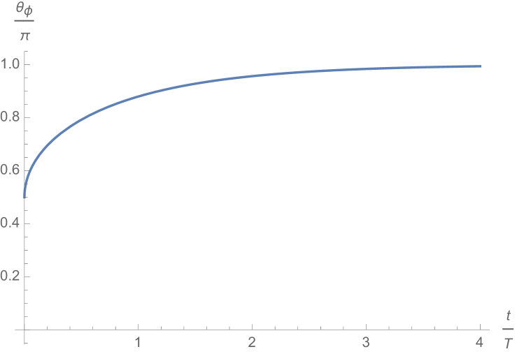
(a) Time evolution of $\theta_{\varphi}$

(b) Time evolution of $c$.

Figure 1: Approximate time evolution of $\theta_{\varphi}$ and $c$ in the second order slow roll regime, where we assume that $\theta_{\varphi}(0)=\frac{\pi}{2}$, i.e. $c(0)=0$. The slow roll curve exits the rapid turn regime after the characteristic time $T\simeq\frac{1}{\sqrt{3V}}$ and enters the infrared regime of [31, 32], which is characterized by $\theta_{\varphi}\approx\pi$ and $c\approx 3$.

Now let us make an improved estimate by taking into account the $V_{\tau\tau}$ term as well. In that case and assuming $V,V_{\tau\tau}\approx\mathrm{const}$ for simplicity, (6.5) has the following solution:

$$\cos\theta_{\varphi}\,\approx\,\pm\,\sqrt{\frac{\hat{C}e^{2\,(A+B)\,t}+A}{\hat{C}e^{2\,(A+B)\,t}-B}}\quad,$$ (6.9)

where $\hat{C}=\mathrm{const}>0$ and we defined:

$$A=\sqrt{3V}\qquad,\qquad B=\frac{V_{\tau\tau}}{\sqrt{3V}}\quad.$$ (6.10)

Again this is not an exact result, since we obtained it by assuming that $A$ and $B$ are constant. But it gives important insights. Namely, the characteristic time is $T=\frac{1}{A+B}=\frac{\sqrt{3V}}{3V+V_{\tau\tau}}$ . Clearly, we can vary $T$ by varying $V$ and $V_{\tau\tau}$ . In any case, though, we have $\cos\theta_{\varphi}\rightarrow\pm 1$ as $t$ increases, i.e. we again have $|\sin\theta_{\varphi}|\rightarrow 0$ for large enough $t$ . If $\theta_{\varphi}(0)=\frac{\pi}{2}$ , then $\dot{\theta}_{\varphi}>0$ in accordance with (6.6). And if $\theta_{\varphi}(0)=-\frac{\pi}{2}$ , then $\dot{\theta}_{\varphi}<0$ . Thus in both cases $\theta_{\varphi}(t)$ tends to $\pi\mod 2\pi$ with time, which means that the field-space trajectory tends to align with minus the gradient of the potential (see Figure 1). This suggests that the rapid turn phase is only transient, although its duration depends on the particulars of the potential and the field-space metric.

Since during slow roll we have $H\approx\sqrt{V/3}$ , it follows that the number of e-folds produced during the characteristic time (in the above crude approximation with $V,V_{\tau\tau}\approx{\rm const}$) is given by:

$${\cal N}=\int_{0}^{T}H\,\mathrm{d}t\,\approx\,\frac{V}{3V+V_{\tau\tau}}\,\lesssim\,\frac{1}{3}\,\,\,,$$ (6.11)

where the last inequality follows from (3.28). This suggests that generically the rapid turn phase is rather short-lived, likely contained within one or only a few e-folds. Obtaining a sustained rapid turn period (capable of lasting 50 - 60 or so e-folds) would require a rather special choice of potential.

Finally, let us comment on the quantities $f_{n}$ and $f_{\tau}$ , defined in (5.9). To estimate them in the crude approximation of (6.7), let us first compute the following ratios:

$$\frac{\dot{v}_{n}}{v_{n}}\! = \!\!-\eta_{\parallel}H-\dot{\theta}_{\varphi}\tan\theta_{\varphi}\approx H\left(3\tan^{2}\theta_{\varphi}-\eta_{\parallel}\right)\approx\frac{H}{3}\,\eta_{\perp}^{2}\quad,$$

$$\frac{\dot{v}_{\tau}}{v_{\tau}}\! = \!\!-\eta_{\parallel}H-\dot{\theta}_{\varphi}\cot\theta_{\varphi}\approx-H\left(3+\eta_{\parallel}\right)\approx-3H\quad,$$ (6.12)

where we used successively (5.2), (2.9) and (6.7), as well as the slow roll approximation. Substituting (6) in (5.9) gives:

$$f_{n}\approx-\frac{\eta_{\perp}^{2}}{3}\qquad,\qquad f_{\tau}\approx 3\quad.$$ (6.13)

This is a rather crude estimate, relying on the leading behavior of the characteristic angle $\theta_{\varphi}(t)$ for $V,V_{\tau\tau}\approx{\rm const}$ . However, it suggests that satisfying the approximations (5.12) would require a rather special choice of scalar potential.

7 Conclusions

We studied consistency conditions for certain approximations commonly used to search for rapid-turn and slow-roll inflationary trajectories in two-field cosmological models with orientable scalar field space. Such consistency conditions arise from requiring compatibility between the equations of motion and the various relevant approximations. We showed that long-lasting rapid turn trajectories with third order slow roll can arise only in regions of field space, where the scalar potential satisfies (3.27). The latter is a nonlinear second order PDE (with coefficients depending on the field space metric), whose derivation follows solely from the field equations together with approximations (3.7) and (3.9). We also studied the relation between the scalar potential and scalar field metric, which is necessary for the existence of slow-roll circular trajectories in two-field models with rotationally invariant scalar field metric. The relevant condition, given by (4.15), is solely a consequence of imposing the slow roll approximations $\varepsilon\ll 1$ and $|\eta_{\parallel}|\ll 1$ on solutions of the equations of motion under the assumptions of a field-space metric of the form (4.1) and of near-circular trajectories (i.e. trajectories with $r\approx$ const). Finally, we showed that the approximation proposed in [20] (which is a rather special case of the slow-roll and rapid-turn approximation) is compatible with the equations of motion only when the scalar metric and potential satisfy a rather nontrivial consistency condition, namely (5.21) for $\Delta\geq 0$ and (5.22) for $\Delta<0$ , where $\Delta$ is the discriminant of (5.20). The only approximations we used to derive the last conditions are (5.12) and $\varepsilon\ll 1$ .

In principle, the various consistency conditions we have obtained could be (approximately) satisfied numerically for a brief period by appropriate choices of integration constants. But they can only be maintained for a prolonged duration, if they are satisfied functionally. Hence, given how complicated these relations are, they constrain dramatically the form of the scalar potential for a given field space metric, and vice versa. In other words, our consistency conditions constrain severely the classes of two-field models, for which one can hope to find long-lasting rapid-turn and slow-roll inflationary trajectories. In that sense, our results show that two-field cosmological models, which allow for such trajectories, are non-generic (or ‘rare’, in the language of [33]) in the class of all two-field models. In particular, this shows that the difficulty in finding such models – which was previously noticed in [33] – is already present in the absence of supersymmetry and hence is unrelated to supergravity.

We also studied the time evolution of the characteristic angle of cosmological trajectories in general two-field models. We argued that (in a crude approximation) a slow roll cosmological trajectory with rapid turn tends to align within a short time with the opposite of a gradient flow line of the model. Thus, generically, the solution tends to enter the gradient flow regime of the model before producing a sufficient number of e-folds. This confirms our conclusion that phenomenologically viable inflationary slow roll trajectories with long-lasting rapid turn are highly non-generic in two-field cosmological models.

The above conclusion may be a ‘blessing in disguise’, since finding such rare trajectories could be more predictive (than if they were generic) and might lead to some deep insights about the embedding of these effective multifield models into an underlying fundamental framework. We hope to investigate in the future what properties of the scalar potential are implied by the consistency conditions found here, as well as to look for ways of solving those conditions even if only for very special choices of scalar metric. In view of [40], it is also worth exploring the consequences of transient violations of slow roll in our context.

Appendix A Derivatives of the adapted frame

Since $n$ is normalized, we have $\nabla_{n}(n_{K}n^{K})=0$ . Hence $\nabla_{n}n=n^{I}\nabla_{I}n$ does not have a component along the vector $n$ . To compute its component along the vector $\tau$ , let us contract it with $\tau$:

$$\tau_{J}n^{I}\nabla_{I}n^{J}=\tau_{J}n^{I}\frac{G^{JK}\nabla_{I}V_{K}}{\sqrt{V_{L}V^{L}}}+\tau_{J}n^{I}G^{JK}V_{K}\nabla_{I}\!\left(\frac{1}{\sqrt{V_{L}V^{L}}}\right)\,\,\,,$$ (A.1)

where we used (3.1) inside $\nabla_{I}n^{J}$ . Substituting (3.2) in the second term of (A.1) gives:

$$\tau_{J}\nabla_{n}n^{J}=\frac{\tau^{K}n^{I}\nabla_{I}V_{K}}{\sqrt{V_{L}V^{L}}}+\sqrt{\det G}\,\epsilon_{JM}\,n^{M}n^{I}V^{J}\nabla_{I}\!\left(\frac{1}{\sqrt{V_{L}V^{L}}}\right)=\frac{V_{n\tau}}{\sqrt{V_{L}V^{L}}}\,\,\,,$$ (A.2)

where in the second equality we used the relation $\epsilon_{JM}\,n^{M}V^{J}=\epsilon_{JM}V^{M}V^{J}/\sqrt{V_{L}V^{L}}=0$, which follows from (3.1). In conclusion, we have

$$\nabla_{n}n\,=\,\frac{V_{n\tau}}{\sqrt{V_{I}V^{I}}}\,\,\tau\,\,\,.$$ (A.3)

One can prove the remaining three relations in (5.1) in a similar manner.

Appendix B Example: Quasi-single field inflation

The goal of this appendix is to demonstrate in a simple example how our consistency conditions can help identify the parts of field space (and/or parameter space) in which a desired type of inflationary solutions can exist and how to determine suitable forms of the scalar potential. We will not delve into the phenomenology of any particular solution, as this would take us too far afield from the subject of this paper. However, by studying the relevant consistency condition for a type of inflationary trajectories, we will show that one can derive constraints on the scalar field space of the model and/or find scalar potentials, which can support the desired inflationary regime.

For this purpose, we consider the class of models of quasi-single field inflation studied in [41]. The field space metric and scalar potential of these models are given respectively by:

$$ds^{2}_{G}=dr^{2}+f(r)d\theta^{2}$$ (B.1)

and

$$V(r,\theta)\,=\,3\left(W^{2}(\theta)-\frac{2W^{2}_{\theta}(\theta)}{3f(r)}\right)\left[1+\frac{\lambda}{2}(r-r_{0})^{2}+\frac{\alpha}{6}(r-r_{0})^{3}+...\right]^{2}\,\,\,,$$ (B.2)

where $f(r)$ and $W(\theta)$ are arbitrary positive functions and $\alpha,\lambda,r_{0}=\mathrm{const}$ . In this context, one can realize orbital inflation with field-space trajectories satisfying:

$$r=r_{0}\,\,\,,$$ (B.3)

and thus having $\dot{r}=0$ identically; for more details, see [41] and references therein. This allows us to apply the consistency condition of Subsection 4.1, which is valid for slow-rolling (near-)circular inflationary trajectories.

$\bullet$  Slow-rolling circular trajectories:

To apply the consistency condition (4.15) to the above class of models, note first that comparing (B.1) and (4.1) implies the identification $h^{2}(r)=f(r)$ . Hence, in terms of $f$ , (4.15) becomes:

$$\frac{1}{6}\frac{f_{r}}{f^{2}}\frac{V_{\theta}^{2}}{V_{r}}\approx V\,\,\,.$$ (B.4)

Let us now evaluate the two sides of this relation on trajectories satisfying (B.3) in the above model. Substituting (B.2) in (B.4), we find for the left-hand side:

$$\frac{1}{6}\frac{f_{r}}{f^{2}}\frac{V_{\theta}^{2}}{V_{r}}\bigg{|}_{r=r_{0}}=\,3\left(W-\frac{2}{3}\frac{W_{\theta\theta}}{f(r_{0})}\right)^{2}\,\,\,,$$ (B.5)

while the right-hand side gives:

$$V|_{r=r_{0}}\,=\,3\left(W^{2}-\frac{2}{3}\frac{W_{\theta}^{2}}{f(r_{0})}\right)\,\,\,.$$ (B.6)

To study numerically certain phenomenological predictions of this kind of model, ref. [41] considered the specific choice of functions:

$$W(\theta)=C_{0}\theta\qquad{\rm and}\qquad f(r)=r^{2}\,\,\,,$$ (B.7)

where $C_{0}=\mathrm{const}$ . Using these in (B.5) and (B.6), we obtain:

$$\frac{1}{6}\frac{f_{r}}{f^{2}}\frac{V_{\theta}^{2}}{V_{r}}\bigg{|}_{r=r_{0}}=\,3C_{0}^{2}\theta^{2}$$ (B.8)

and

$$V|_{r=r_{0}}\,=\,3C_{0}^{2}\theta^{2}-2\frac{C_{0}^{2}}{r_{0}^{2}}\,\,\,.$$ (B.9)

Clearly, the last two expressions are never equal. But they can be sufficiently numerically close to each other if the extra term in (B.9) is small enough, namely if:

$$\theta^{2}\gg\frac{2}{3r_{0}^{2}}\,\,\,.$$ (B.10)

Whether this condition can be satisfied or not (and for how long) depends on the initial conditions of the trajectory under consideration. In any case, satisfying (B.10) requires a certain level of fine-tuning of the inflationary model.

Alternatively, instead of using the ad hoc choice (B.7), we can solve the consistency condition (B.4) functionally. This will enable us to find suitable pairs of functions $W$ and $f$  which are compatible with solutions of the equations of motion in the slow roll regime. In view of (B.5) and (B.6), on the trajectories of interest relation (B.4) has the form:

$$\left(W(\theta)-\frac{2}{3}\frac{W_{\theta\theta}}{f(r_{0})}\right)^{2}=\,W^{2}(\theta)-\frac{2}{3}\frac{W_{\theta}^{2}}{f(r_{0})}\,\,\,.$$ (B.11)

We now view (B.11) as an ODE for $W(\theta)$ , given a function $f(r_{0})$ . The solutions of this equation are:

$$W_{1}(\theta)=\frac{1}{2}C_{1}\theta^{2}+C_{0}\theta+\frac{1}{3}\frac{C_{1}}{f(r_{0})}+\frac{1}{2}\frac{C_{0}^{2}}{C_{1}}\qquad{\rm and}\qquad W_{2,3}(\theta)=e^{\pm\frac{\sqrt{6}}{2}\sqrt{f(r_{0})}\,(\theta-C_{2,3})}\,\,\,,$$ (B.12)

where $C_{0,1,2,3}=\mathrm{const}$ and $C_{1}\neq 0$ . Note that substituting $W_{2,3}(\theta)$ in (B.6) leads to $V|_{r=r_{0}}=0$ . Hence these two solutions should be discarded due to the requirement to have a positive potential on inflationary trajectories. So only $W_{1}(\theta)$ is an acceptable solution in the present context. For later convenience, let us record its special case with $C_{0}=0$ :

$$W(\theta)=\frac{1}{2}C_{1}\theta^{2}+\frac{1}{3}\frac{C_{1}}{f(r_{0})}\,\,\,.$$ (B.13)

To summarize, we have shown, in principle, how the consistency conditions (in this example: for the existence of circular slow-roll trajectories) can either restrict the field (or parameter) space of an inflationary model, as in (B.10), or fix the form of the potential (for a given field-space metric), as in (B.12). This illustrates manifestly, albeit on a technically much simpler example than in Sections 3 and 5, how our consistency conditions can play a constructive role in inflationary model building.

$\bullet$  Rapid turn regime:

Although rapid turn inflation was not discussed in [41], for our purposes it is interesting to investigate whether slow-roll circular trajectories in this kind of model can exhibit rapid turning in some parts of the field (and/or parameter) space. To address this question, we now consider the dimensionless turn rate $\eta_{\perp}=\Omega/H$ of such trajectories.

The turn rate of any background trajectory in a cosmological model with field-space metric (B.1) is given by [11]:

$$\Omega\,=\,\frac{\sqrt{f}}{(\dot{r}^{2}+f\dot{\theta}^{2})}\left(\dot{\theta}V_{r}-\frac{\dot{r}}{f}V_{\theta}\right)\,\,\,.$$ (B.14)

Also, the above quasi-single field models with potential (B.2) have a Hubble parameter of the form [41]:

$$H(r,\theta)\,=\,W(\theta)\left(1+\frac{\lambda}{2}(r-r_{0})^{2}+\frac{\alpha}{6}(r-r_{0})^{3}+...\right)\,\,\,,$$ (B.15)

and exact inflationary solutions satisfying (B.3) and [41] (see also [42]):

$$\dot{\theta}=-2\,\frac{H_{\theta}}{f}\,\,\,.$$ (B.16)

These solutions are not automatically slow-rolling, as will become clear below. Note also that (B.15) implies  $H|_{r=r_{0}}\!=\!W$ ; thus the requirement for positive $W$ that we mentioned earlier. Let us now compute the turn rate of the respective trajectories. Recall that, due to (B.3) , along those trajectories $\dot{r}=0$ identically. Hence, using (B.2) and (B.14)-(B.16), we find:

$$\Omega|_{r=r_{0}}\,=\,\frac{V_{r}}{\sqrt{f}\dot{\theta}}\bigg{|}_{r=r_{0}}=-\frac{W_{\theta}\,f_{r}}{f^{3/2}}\bigg{|}_{r=r_{0}}$$ (B.17)

and thus

$$\eta_{\perp}|_{r=r_{0}}=\frac{\Omega}{H}\bigg{|}_{r=r_{0}}=-\frac{W_{\theta}\,f_{r}}{f^{3/2}\,W}\bigg{|}_{r=r_{0}}\,\,\,.$$ (B.18)

Let us now apply (B.18) to the two examples discussed above. First we consider the choice (B.7). In that case, (B.18) gives:

$$\eta_{\perp}|_{r=r_{0}}\,=\,-\,\frac{2}{r_{0}^{2}\,\theta}\,\,\,.$$ (B.19)

Hence the rapid turn condition $\eta_{\perp}^{2}\gg 1$ implies:

$$\frac{4}{r_{0}^{4}\,\theta^{2}}\,\gg\,1\,\,\,.$$ (B.20)

Combining this with (B.10), we find:

$$\frac{2}{3}\,r_{0}^{2}\,\ll\,r_{0}^{4}\,\theta^{2}\ll 4\,\,\,,$$ (B.21)

which means in particular that:

$$r_{0}^{2}\ll 6\,\,\,.$$ (B.22)

In other words, we have derived constraints on both the parameter space of the model and the part of its field space, where the trajectories of slow-roll rapid-turn inflationary solutions could lie. These constraints point to different regions of field/parameter space than those whose phenomenology was studied numerically in [41, 42]. In these references, the numerical computations were performed with $r_{0}^{2}>1$ to ensure perturbative control and to avoid numerical instabilities (see especially [42]). Whether the constraints (B.21) can lead to phenomenologically viable inflationary models is an interesting question for the future.

Now let us compute (B.18) for a function $W(\theta)$ , which solves the consistency condition (B.11). For simplicity, we consider the special case (B.13). Substituting this $W$ in (B.18) gives:

$$\eta_{\perp}|_{r=r_{0}}\,=\,-\,\frac{2\,\theta f_{r}(r_{0})}{f^{3/2}(r_{0})\left(\theta^{2}+\frac{2}{3f(r_{0})}\right)}\,\,\,.$$ (B.23)

Hence the rapid turn condition becomes:

$$\eta_{\perp}^{2}|_{r=r_{0}}\,=\,\frac{4\,\theta^{2}f_{r}^{2}}{f^{3/2}\left(\theta^{2}+\frac{2}{3f}\right)^{\!2}}\Bigg{|}_{r=r_{0}}\,\gg\,1\,\,\,.$$ (B.24)

Note that so far the function $f$ has been arbitrary. This gives us a lot of freedom in how to satisfy (B.24). In particular, one can easily choose $f(r)$ such that the slow-roll and rapid-turn regime occurs for $r_{0}^{2}>1$ , in which case one could use the same numerical methods as in [41, 42] to study the phenomenology of the resulting model. Clearly there is an unlimited number of interesting choices for $f$ . We do not claim that any of them would be better than known models and/or would be compatible with further phenomenological requirements (nor with the third order slow roll conditions of Section 3); this is a topic for future studies. Our aim here was merely to illustrate in principle, and on a very simple example, how our consistency conditions could be a valuable guide in inflationary model building.

The discussion in this Appendix shows, furthermore, that these consistency conditions could provide a rich source of ideas for the development of new models or, at the very least, tractable toy models, which could help elucidate important features of rapid turn inflation.

References

- [1] S. Garg, C. Krishnan, Bounds on Slow Roll and the de Sitter Swampland, JHEP 11 (2019) 075, arXiv:1807.05193 [hep-th].
- [2] H. Ooguri, E. Palti, G. Shiu, C. Vafa, Distance and de Sitter Conjectures on the Swampland, Phys. Lett. B 788 (2019) 180, arXiv:1810.05506 [hep-th].
- [3] A. Achucarro, G. Palma, The string swampland constraints require multi-field inflation, JCAP 02 (2019) 041, arXiv:1807.04390 [hep-th].
- [4] R. Bravo, G. A. Palma, S. Riquelme, A Tip for Landscape Riders: Multi-Field Inflation Can Fulfill the Swampland Distance Conjecture, JCAP 02 (2020) 004, arXiv:1906.05772 [hep-th].
- [5] C. M. Peterson, M. Tegmark, Testing Two-Field Inflation, Phys. Rev. D 83 (2011) 023522, arXiv:1005.4056 [astro-ph.CO].
- [6] C. M. Peterson, M. Tegmark, Non-Gaussianity in Two-Field Inflation, Phys. Rev. D 84 (2011) 023520, arXiv:1011.6675 [astro-ph.CO].
- [7] S. Cespedes, V. Atal, G. A. Palma, On the importance of heavy fields during inflation, JCAP 05 (2012) 008, arXiv:1201.4848 [hep-th].
- [8] T. Bjorkmo, R. Z. Ferreira, M.C.D. Marsh, Mild Non-Gaussianities under Perturbative Control from Rapid-Turn Inflation Models, JCAP 12 (2019) 036, arXiv:1908.11316 [hep-th].
- [9] G. A. Palma, S. Sypsas, C. Zenteno, Seeding primordial black holes in multi-field inflation, Phys. Rev. Lett. 125 (2020) 121301, arXiv:2004.06106 [astro-ph.CO].
- [10] J. Fumagalli, S. Renaux-Petel, J. W. Ronayne, L. T. Witkowski, Turning in the landscape: a new mechanism for generating Primordial Black Holes, arXiv:2004.08369 [hep-th].
- [11] L. Anguelova, On Primordial Black Holes from Rapid Turns in Two-field Models, JCAP 06 (2021) 004, arXiv:2012.03705 [hep-th].
- [12] L. Anguelova, Primordial Black Hole Generation in a Two-field Inflationary Model, Springer Proc. Math. Stat. 396 (2022) 193, arXiv:2112.07614 [hep-th].
- [13] Y. Akrami, M. Sasaki, A. Solomon and V. Vardanyan, Multi-field dark energy: cosmic acceleration on a steep potential, Phys. Lett. B 819 (2021) 136427, arXiv:2008.13660 [astro-ph.CO].
- [14] L. Anguelova, J. Dumancic, R. Gass, L.C.R. Wijewardhana, Dark Energy from Inspiraling in Field Space, JCAP 03 (2022) 018, arXiv:2111.12136 [hep-th].
- [15] A Brown, Hyperinflation, Phys. Rev. Lett. 121 (2018) 251601, arXiv:1705.03023 [hep-th].
- [16] S. Mizuno, S. Mukohyama, Primordial perturbations from inflation with a hyperbolic field-space, Phys. Rev. D 96 (2017) 103533, arXiv:1707.05125 [hep-th].
- [17] P. Christodoulidis, D. Roest, E. Sfakianakis, Angular inflation in multi-field -attractors, JCAP 11 (2019) 002, arXiv:1803.09841 [hep-th].
- [18] S. Garcia-Saenz, S. Renaux-Petel, J. Ronayne, Primordial fluctuations and non-Gaussianities in sidetracked inflation, JCAP 1807 (2018) 057, arXiv:1804.11279 [astro-ph.CO].
- [19] A. Achucarro, E. Copeland, O. Iarygina, G. Palma, D.G. Wang, Y. Welling, Shift-Symmetric Orbital Inflation: single field or multi-field?, Phys. Rev. D 102 (2020) 021302, arXiv:1901.03657 [astro-ph.CO].
- [20] T. Bjorkmo, The rapid-turn inflationary attractor, Phys. Rev. Lett. 122 (2019) 251301, arXiv:1902.10529 [hep-th].
- [21] T. Bjorkmo, M. C. D. Marsh, Hyperinflation generalised: from its attractor mechanism to its tension with the ‘swampland conditions’, JHEP 04 (2019) 172, arXiv:1901.08603 [hep-th].
- [22] V. Aragam, S. Paban, R. Rosati, The Multi-Field, Rapid-Turn Inflationary Solution, JHEP 03 (2021) 009, arXiv:2010.15933 [hep-th].
- [23] Y. Zhang, Y.-g. Gong, Z.-H. Zhu, Noether Symmetry Approach in multiple scalar fields Scenario, Phys. Lett. B688 (2010) 13, arXiv:0912.0067 [hep-ph].
- [24] A. Paliathanasis, M. Tsamparlis, Two scalar field cosmology: Conservation laws and exact solutions, Phys. Rev. D 90 (2014) 043529, arXiv:1408.1798 [gr-qc].
- [25] L. Anguelova, E.M. Babalic, C.I. Lazaroiu, Two-field Cosmological -attractors with Noether Symmetry, JHEP 1904 (2019) 148, arXiv:1809.10563 [hep-th].
- [26] L. Anguelova, E.M. Babalic, C.I. Lazaroiu, Hidden symmetries of two-field cosmological models, JHEP 09 (2019) 007, arXiv:1905.01611 [hep-th].
- [27] C. I. Lazaroiu, Hesse manifolds and Hessian symmetries of multifield cosmological models, Rev. Roumaine Math. Pures Appl. 66 (2021) 2, 329-345, arXiv:2009.05117 [hep-th].
- [28] C. I. Lazaroiu, C. S. Shahbazi, Generalized two-field -attractor models from geometrically finite hyperbolic surfaces, Nucl. Phys. B 936 (2018) 542-596, arXiv:1702.06484 [hep-th].
- [29] E. M. Babalic, C. I. Lazaroiu, Generalized -attractor models from elementary hyperbolic surfaces, Adv. Math. Phys. 2018 (2018) 7323090, arXiv:1703.01650 [hep-th].
- [30] E. M. Babalic, C. I. Lazaroiu, Generalized -attractors from the hyperbolic triply-punctured sphere, Nucl. Phys. B 937 (2018) 434-477, arXiv:1703.06033 [hep-th].
- [31] C. I. Lazaroiu, Dynamical renormalization and universality in classical multifield cosmological models, Nucl. Phys. B 983 (2022) 115940, arXiv:2202.13466 [hep-th].
- [32] E. M. Babalic, C. I. Lazaroiu, The infrared behavior of tame two-field cosmological models, Nucl. Phys. B 983 (2022) 115929, arXiv:2203.02297 [gr-qc].
- [33] V. Aragam, R. Chiovoloni, S. Paban, R. Rosati, I. Zavala, Rapid-turn inflation in supergravity is rare and tachyonic, JCAP 03 (2022) 002, arXiv:2110.05516 [hep-th].
- [34] A, R. Liddle, P. Parsons, J. D. Barrow, Formalizing the slow-roll approximation in inflation, Phys. Rev. D 50 (1994) 7222, arXiv:astro-ph/9408015.
- [35] A. Hetz, G. Palma, Sound Speed of Primordial Fluctuations in Supergravity Inflation, Phys. Rev. Lett. 117 (2016) 101301, arXiv:1601.05457 [hep-th].
- [36] A. Achucarro, J.-O. Gong, S. Hardeman, G. Palma, S. Patil, Features of heavy physics in the CMB power spectrum, JCAP 01 (2011) 030, arXiv:1010.3693 [hep-ph].
- [37] D. Chakraborty, R. Chiovoloni, O. Loaiza-Brito, G. Niz, I. Zavala, Fat inflatons, large turns and the -problem, JCAP 01 (2020) 020, arXiv:1908.09797 [hep-th].
- [38] P. Christodoulidis, D. Roest, E. Sfakianakis, Attractors, Bifurcations and Curvature in Multi-field Inflation, JCAP 08 (2020) 006, arXiv:1903.03513 [gr-qc].
- [39] P. Christodoulidis, D. Roest, E. Sfakianakis, Scaling attractors in multi-field inflation, JCAP 12 (2019) 059, arXiv:1903.06116 [hep-th].
- [40] S. Bhattacharya, I. Zavala, Sharp turns in axion monodromy: primordial black holes and gravitational waves, arXiv:2205.06065 [astro-ph.CO].
- [41] Y. Welling, A simple, exact, model of quasi-single field inflation, Phys. Rev. D 101, 063535 (2020), arXiv:1907.02951 [astro-ph.CO].
- [42] A. Achucarro, Y. Welling, Orbital Inflation: inflating along an angular isometry of field space, arXiv:1907.02020 [hep-th].