Abstract

We investigate the generation and transfer of entangled states between two coupled microtoroidal cavities considering two different types of couplings, namely i) via a bridge qubit and ii) via evanescent fields. The cavities support two counter-propagating whispering-gallery modes (WGMs) that may also interact with each other. We firstly show that it is possible to transfer, with high fidelity, a maximally entangled state between the two modes of the first cavity (cavity $1$) to the two modes of the second cavity (cavity $2$), independently of the type of coupling. Interesting differences, though, arise concerning the generation of entangled states from initial product states; if the cavities are coupled via a bridge qubit, we show that it is possible to generate a 4-partite entangled state involving all four cavity modes. On the other hand, contrarily to what happens in the qubit coupling case, it is possible to generate bipartite maximally entangled states between modes of different cavities from initial separable states for cavities coupled by evanescent waves. Besides, we show that different entangled states between the propagating and counter-propagating modes of distinct cavities may be generated by tuning the interaction between modes belonging to the same cavity (intra-cavity couplings). Again, this is possible only for the couplings via evanescent waves. For the completion of our work, we discuss the effects of losses on the dynamics of the system.

Generation and transfer of entangled states between two connected microtoroidal cavities: analysis of different types of coupling

Emilio H. S. Sousa^(a,b), A. Vidiella-Barranco^(b) and J. A. Roversi^(b)

1 Introduction

Quantum entanglement is a fundamental resource and also indispensable in many important applications such as quantum key distribution [1, 2], quantum computing [3], dense coding [4], and quantum information processing [5]. For instance, the performance of tasks such as quantum teleportation in a quantum network, depends on both the control of entanglement generation and the transfer of entangled states between distant parties [6]. Several theoretical and experimental works have shown that cavity QED systems promote an efficient route towards the generation and distribution of entanglement [7, 8, 9, 10]. In [11], the authors have demonstrated a process of entanglement transfer engineering, where two remote qubits interact with an entangled two-mode continuous-variable field. Whereas the authors in [12] used a single superconducting qubit to induce entanglement between two separated transmission line resonators, in [13] the authors introduce two gap-tunable superconducting qubits to generate a two-mode entangled state through dissipation. The generation of two-mode entangled states using superconducting qubits has also been studied in [14, 15], while in [16] the authors proposed the use of a bridge qubit to couple cavities containing each one a qubit. We remark that the coupling via a bridge qubit would allow the adjustment of the interaction between the two microtoroidal cavities (including to switch it on/off), which is of importance for the scalability of quantum circuits [16]. In [17], the authors used a single circular Rydberg atom to prepare two-modes of the field of a superconducting cavity in a maximally entangled state, while in [18] the authors have proposed the creation of maximally entangled states for two modes via a single atom resonating with an ultra-high $Q$ microtoroidal cavity. The preparation of a steady entangled state between two separated nitrogen-vacancy (NV) centers attached to the outer surface of two microtoroidal cavities coupled by a WGM field has been proposed in [19]. In [20], the authors showed that it is possible to produce a steady entangled state of the two NV centers with two WGM microresonators, coupled either by an optical fiber-taper or via evanescent fields.

To our knowledge though, the investigation and comparison of different couplings between two WGMs microtoroidal cavities aiming at the entanglement generation and transfer of two-mode entangled states has not yet been addressed in the literature. Here, we report protocols of generation and transfer of entangled states between two coupled microtoroidal cavities, considering setups with two different types of inter-cavity couplings, namely: i) a bridge qubit; and ii) evanescent waves. Each one of the cavities supports two counter-propagating WGMs, clockwise and counterclockwise propagating modes, that may be coupled to each other due the cavity imperfections [21, 22]. We are interested in the investigation of the effects of different couplings on the dynamics of entanglement of the WGMs in the cavities, as well as in the control of the generation of entangled states by tuning the parameters of the system. We show that it is possible to transfer, with high fidelity, a maximally entangled state between the two-modes of the first cavity to the modes of the second cavity for each one of the considered couplings. In particular, the transfer of entangled states between cavities is independent of the interaction between the intra-cavity modes if the cavities are coupled via evanescent waves. Concerning the possibilities of generation of entangled states from initial product states, we find that in the case of the evanescent waves coupling, bipartite maximally entangled states involving different modes may be generated, depending on the interaction between the intra-cavity modes. This allows the selection of the generated states by tuning the aforementioned interactions. Yet, such flexibility is not possible if the cavities are coupled via a bridge qubit. Nonetheless, we show that precisely in the case of coupling via a qubit, it is possible to generate a 4-partite entangled state involving the four cavity field states. Thus, in this system of two microtoroidal cavities, each of the cavity-cavity couplings considered here has particular features which would allow the transfer and generation of a wide range of entangled states of the quantized field. For completeness, we investigate the influence of losses on the dynamics of entanglement in the system.

Our paper is organized as follows. Firstly, in Section 2, we present the models and descriptions of the physical systems. In Section 3, we investigate and discuss the transfer and generation of entanglement (quantified by the Concurrence) for different types of couplings and different initial states. The effects of losses are discussed in Section 4. Finally, we summarize our conclusions in Section 5.

2 Models of two coupled microtoroidal cavities

Consider a system composed of two separate toroidal cavities, each one supporting two whispering gallery counter-propagating modes (WGM’s) of frequencies $\omega_{ci}$ $(i=1,2)$ with corresponding photon annihilation (creation) operators given by $a_{i}$ ($a_{i}^{\dagger}$) and $b_{i}$ ($b_{i}^{\dagger}$). We also assume an interaction between the two WGMs (with intra-cavity coupling constants $J_{i}$) induced by small deformations in the toroid [21, 22]. Hence, the Hamiltonian of such a system will read:

$$H_{S} = \hbar\omega_{c1}(a_{1}^{\dagger}a_{1}+b_{1}^{\dagger}b_{1})+\hbar\omega_{c2}(a_{2}^{\dagger}a_{2}+b_{2}^{\dagger}b_{2})$$ (1)

$$+ \hbar J_{1}(a_{1}^{\dagger}b_{1}+b_{1}^{\dagger}a_{1})+\hbar J_{2}(a_{2}^{\dagger}b_{2}+b_{2}^{\dagger}a_{2}).$$

Here, we suppose that the cavities can be connected using two different types of coupling (one at a time), namely: i) via a bridge qubit, i.e., a two-level system, which can be an artificial atom, a nitrogen vacancy center, etc., having transition frequency $\omega_{a}$; and ii) via evanescent waves.

In the bridge qubit case, as shown in Fig. 1, we consider that the two WGMs counter-propagating modes of each cavity are simultaneously coupled to the qubit with coupling constants $g_{i}$. Thus, the total Hamiltonian with the additional interaction term has the form:

$$H_{T}=H_{S}+H_{g},$$ (2)

where

$$H_{g} = \hbar\omega_{a}\sigma^{+}\sigma^{-}+\hbar g_{1}(a_{1}^{\dagger}\sigma^{-}+a_{1}\sigma^{+})+\hbar g_{1}(b_{1}^{\dagger}\sigma^{-}+b_{1}\sigma^{+})$$ (3)

$$+ \hbar g_{2}(a_{2}^{\dagger}\sigma^{-}+a_{2}\sigma^{+})+\hbar g_{2}(b_{2}^{\dagger}\sigma^{-}+b_{2}\sigma^{+}).$$

Here $\sigma^{+}$ and $\sigma^{-}$ are the raising and lowering operators of the qubit.

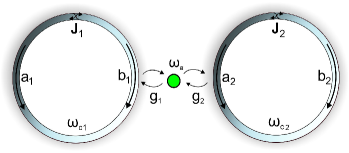
Figure 1: A schematic illustration showing the setup of two toroidal cavities supporting modes $a_{1}\wedge b_{1}$ and $a_{2}\wedge b_{2}$, coupled via a brigde qubit, with coupling constants $g_{1}=g_{2}\equiv g$.

If the two cavities are coupled via evanescent fields as shown in Fig. 2, the total Hamiltonian with the additional term has the form:

$$H_{T}=H_{S}+H_{\lambda},$$ (4)

where

$$H_{\lambda}=\hbar\lambda(e^{-i\phi}a_{1}^{\dagger}b_{2}+e^{i\phi}b_{2}^{\dagger}a_{1}+e^{-i\phi}b_{1}^{\dagger}a_{2}+e^{i\phi}a_{2}^{\dagger}b_{1}).$$ (5)

Here $\lambda$ is the effective coupling constant between the connected cavities. Such a direct coupling is due to a coherent photon exchange (at a rate $\lambda$) that may occur in several optical systems [23]. The phase $\phi$ is related to the propagation distance between the microtoroids. In order to avoid delaying effects in the photon propagation, a short distance limit between the toroids should be imposed (here we take $\phi=0$).

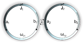
Figure 2: A schematic illustration showing the setup of two toroidal cavities supporting modes $a_{1}\wedge b_{1}$ and $a_{2}\wedge b_{2}$, coupled directly via evanescent waves, with coupling constant $\lambda$.

3 Results: transfer and generation of entangled states

In what follows, we will discuss the transfer of entanglement as well as the generation of entangled states in the two-cavity system, considering each one of the couplings presented above.

3.1 Entangled state transfer

We would like now to investigate under which conditions we are able to transfer an entangled state of the field modes in cavity $1$ to the field modes in cavity $2$. Firstly we consider the case of coupling via a bridge qubit with the following initial conditions: the two modes of cavity $1$ prepared in an entangled state, the qubit in its ground state and the two modes of cavity $2$ in their vacuum states

$$|\Psi(0)\rangle_{g}=(\cos\theta|10\rangle+\sin\theta|01\rangle)_{c1}|g\rangle|00\rangle_{c2}.$$ (6)

Our transmission protocol should work in such a way that entanglement would be transferred from cavity $1$ to cavity $2$ in the following way:

$$|\Psi(0)\rangle_{g} = \left(\cos\theta|10\rangle+\sin\theta|01\rangle_{c1}\right)|g\rangle|00\rangle_{c2}$$

$$\Rightarrow |\Psi^{\prime}\rangle_{g}=|00\rangle_{c1}|g\rangle\left(\cos\theta|10\rangle+\sin\theta|01\rangle\right)_{c2}.$$

Thus, if we depart from the initial state in Eq.(6), the time-evolved state of the system using the Hamiltonian in Eq. (2) (coupling via a bridge qubit) is

$$|\Psi(t)\rangle_{g}=G_{1}(t)|10g00\rangle+G_{2}(t)|01g00\rangle+G_{3}(t)|00e00\rangle+G_{4}(t)(|00g10\rangle+|00g01\rangle),$$ (8)

where

$$G_{1}(t)=\frac{1}{4}\left[{2\emph{e}}^{-\alpha t}(\cos\theta-\sin\theta)+\Gamma+\beta\right],$$ (9)

$$G_{2}(t)=\frac{1}{4}\left[{2\emph{e}}^{-\alpha t}(\sin\theta-\cos\theta)+\Gamma+\beta\right],$$ (10)

$$G_{3}(t)=\frac{2\textit{i}\Gamma\emph{e}^{-\alpha t/2}\sinh(\Delta^{2}gt/2)}{\Delta^{2}}$$ (11)

and

$$G_{4}(t) = \frac{(\cos\theta+\sin\theta)\emph{e}^{(\alpha-\Delta^{2}g)t/2}}{8g\Delta^{2}}$$

$$\times \left[\textit{i}(\emph{e}^{\Delta^{2}gt}-1)J+(1+\emph{e}^{\Delta^{2}gt}-2\emph{e}^{(\alpha+\Delta^{2}g)t/2})\Delta^{2}g\right],$$

with $\alpha=\textit{i}J,\qquad\Gamma=\emph{e}^{\alpha t}(\cos\theta+\sin\theta),\qquad\Delta=\sqrt{\textit{i}[16+(J/g)^{2}]}\qquad$ and

$$\beta=\frac{1}{\Delta^{2}}\left\{\emph{e}^{\alpha t/2}(\cos\theta+\sin\theta)\left[\Delta^{2}\cosh(\Delta^{2}gt)+\textit{i}J\sinh(\Delta^{2}gt)/g\right]\right\}.$$ (13)

For the coupling via evanescent waves, the initial state will read

$$|\Phi(0)\rangle_{\lambda}=(\cos\theta|10\rangle+\sin\theta|01\rangle)_{c1}|00\rangle_{c2},$$ (14)

with the corresponding transmission protocol

$$|\Phi(0)\rangle_{\lambda} = \left(\cos\theta|10\rangle+\sin\theta|01\rangle\right)_{c1}|00\rangle_{c2}$$

$$\Rightarrow |\Phi^{\prime}\rangle_{\lambda}=|00\rangle_{c1}\left(\cos\theta|10\rangle+\sin\theta|01\rangle\right)_{c2}.$$

In this case (evanescent waves) with initial state in Eq.(14), the time-evolved state of the system using the Hamiltonian in Eq. (4) reads

$$|\Phi(t)\rangle_{\lambda}=W_{1}(t)|1000\rangle+W_{2}(t)|0100\rangle+W_{3}(t)|0010\rangle+W_{4}(t)|0001\rangle,$$ (16)

where

$$W_{1}(t)=\cos(\lambda t)[\cos\theta\cos(J\lambda t)+\textit{i}\cos\theta\sin(J\lambda t)],$$ (17)

$$W_{2}(t)=\cos(\lambda t)[\sin\theta\cos(J\lambda t)+\textit{i}\sin\theta\sin(J\lambda t)],$$ (18)

$$W_{3}(t)=\sin(\lambda t)[\textit{i}\cos\theta\cos(J\lambda t)-\sin\theta\sin(J\lambda t)],$$ (19)

and

$$W_{4}(t)=\sin(\lambda t)[\textit{i}\cos\theta\sin(J\lambda t)-\cos\theta\sin(J\lambda t)].$$ (20)

Now we are going to find at which times the initial entanglement of the intra-cavity modes in cavity $1$ (between the $a_{1}\wedge b_{1}$ field modes) is fully transferred to the field modes in cavity $2$ ($a_{2}\wedge b_{2}$). For that, we employ the Concurrence function [24], a widely used quantifier of entanglement defined as

$$C(\rho_{j})=\textit{max}\left\{0,\sqrt{\lambda_{1}}-\sqrt{\lambda_{2}}-\sqrt{\lambda_{3}}-\sqrt{\lambda_{4}}\right\},$$ (21)

where $\lambda_{i}$ are the eigenvalues in decreasing order of the non-Hermitian matrix $\rho_{j}\tilde{\rho}_{j}$ of the corresponding bipartitions, with $\tilde{\rho}_{j}=(\sigma_{y}\otimes\sigma_{y}){\rho^{*}_{j}}(\sigma_{y}\otimes\sigma_{y})$. The index $j$ may refer to the density matrix of the system of two cavities coupled via: the qubit $(j=g)$; or evanescent waves $(j=\lambda)$. For instance, the Concurrence of the bipartite state constituted by the fields of cavity 1 is obtained from the reduced density operator $\rho_{j}\equiv\rho^{(a1,b1)}_{j}$, after tracing over the remaining sub-systems, i.e., $\rho^{(a1,b1)}_{g}=\mbox{Tr}_{a2,b2,q}\Big{[}|\Psi\rangle_{g}{}_{g}\langle\Psi|\Big{]}$ (bridge qubit coupling) and $\rho^{(a1,b1)}_{\lambda}=\mbox{Tr}_{a2,b2}\Big{[}|\Phi\rangle_{\lambda}{}_{\lambda}\langle\Phi|\Big{]}$ (evanescent fields coupling). For convenience, we calculated the Concurrence as a function of the normalized time $\tau$, with correspondence to each type of coupling defined as $\tau^{(j)}$: i) $\tau^{(g)}\equiv gt$ (qubit); and ii) $\tau^{(\lambda)}\equiv\lambda t$ (evanescent fields). We should stress that our calculations are compatible with typical experimental values of the relevant parameters [25, 26], that is: $g/2\pi=70$ MHz, $\lambda/2\pi=30$ MHz, and $J_{1,2}$ may vary from $J_{1,2}=0$ to $J_{1,2}/2\pi=250$ MHz. In Fig. 3 we have plots of the Concurrence as a function of the normalized time $\tau$, in relation to the field modes in cavity $1$ ($a_{1}\wedge b_{1}$) as well as as the field modes in cavity $2$ ($a_{2}\wedge b_{2}$). In Fig. 3(a) we considered uncoupled intra-cavity modes, i.e., $J_{1}=J_{2}=0$. In this case, we find that regardless of the type of coupling between cavities, at the specific time $\tau_{2}=\pi/2$ the field modes in cavity $1$ are non-entangled $(C_{a1b1}=0)$, while the field modes in cavity $2$ become maximally entangled, $(C_{a2b2}=1)$, i.e., entanglement is fully transferred from cavity $1$ to cavity $2$. However the degree of entanglement for intermediate times is slightly different in each case, as shown in Fig. 3(a). If the intra-cavity field couplings are nonzero ($J_{1,2}\neq 0$), maximal entanglement in cavity $2$ is still achieved in the evanescent fields case, although this does not occur for the coupling via a bridge qubit, as seen in Fig. 3(b).

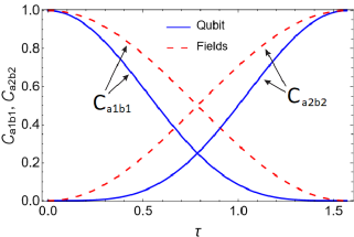
(a)

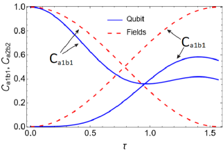
(b)

Figure 3: Concurrence relative to the cavity $1$ ($a_{1}\wedge b_{1}$) and cavity 2 ($a_{2}\wedge b_{2}$) modes, as a function of the normalized time $\tau$, for couplings via: a bridge qubit (blue line, $\tau^{(g)}$); evanescent fields (dashed red line, $\tau^{(\lambda)}$). Intra-cavity modes are uncoupled ($J_{1}=J_{2}=0$) in (a), and coupled in (b), with $J_{1}=J_{2}=2\eta$. Here $\eta=g$ refers to the bridge qubit coupling, and $\eta=\lambda$ to the coupling via evanescent waves.

We would like now to take a more careful look at the bridge qubit coupling case for non-interacting intra-cavity modes ($J_{1,2}=0$) having an initial maximally entangled state in cavity $1$. For that we plot the Concurrence as a function of the normalized time $\tau$, relatively to cavity $1$ modes as well as cavity $2$ modes for two full periods (up to $\tau=2\pi$), as shown in Fig. 4. We clearly see that while entanglement is transferred from cavity $1$ to cavity $2$ at $\tau_{2}=\pi/2$, the cavity $1$ modes are kept with null entanglement during a finite time interval, which characterizes the phenomenon known as Sudden Death of Entanglement (SDE) [27, 28].The entanglement goes down to zero before $\tau_{2}$ and revives after a short time, i.e., a Sudden Rebirth of Entanglement (SRE) occurs. We should point out that both SDE and SRE can take place even if the system is not coupled to an environment with many degrees of freedom, as discussed in [29]. Since the evolution of entanglement is periodic, the Concurrence of the field modes in cavity $1$ returns to its maximum value $C=1.0$ at $\tau_{3}=\pi$. However, the entanglement with respect to the field modes $a_{2}\wedge b_{2}$ goes to zero before $\tau_{3}=\pi$, remaining null for a finite time interval, i.e., SDE also takes place in the field modes of cavity $2$, as seen in Fig. 4. Yet, the SDE/SRE does not occur in a coupling via evanescent fields, emerging only if the cavities are connected via a bridge qubit.

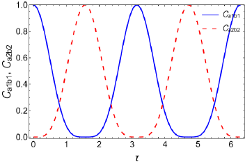
Figure 4: Concurrence as a function of the normalized time $\tau$ (showing “sudden death") relatively to the field modes in cavity $1$ ($a_{1}\wedge b_{1}$) and in cavity $2$ ($a_{2}\wedge b_{2}$) for a bridge qubit coupling, with $g_{1}=g_{2}=g$ and $J_{1}=J_{2}=0$. The initial state of the system is $|{\psi(0)}\rangle=\frac{1}{\sqrt{2}}(|10\rangle+|01\rangle)_{c1}|g\rangle|00\rangle_{c2}$.

3.2 Entangled state generation

In this section we are going to discuss the generation of entangled states involving the sub-systems available: the qubit (in the case of coupling via a qubit), and the WGMs.

3.2.1 Coupling via a bridge qubit

Firstly we discuss the generation of entangled states involving the propagating and counter-propagating modes of distinct cavities and the bridge qubit. In this case we assume an initial preparation of the system in the state $|\Psi(0)\rangle=(\cos\theta|10\rangle+\sin\theta|01\rangle)_{c1}|g\rangle|00\rangle_{c2}$. Then, if the evolution of the system is governed by the Hamiltonian in Eq. (2) from an initial product state $(\theta=0)$ with non-interacting intra-cavity modes $(J_{1,2}=0)$, we find that the state of the system at a time $\tau_{2}=\pi/2$ will be the following 4-partite entangled state

$$|\Psi(\tau=\pi/2,\theta=0,J_{1,2}=0)\rangle=$$

$$=\frac{1}{2}\big{(}|1\rangle_{a1}|0\rangle_{b1}|0\rangle_{a2}|0\rangle_{b2}+|0\rangle_{a1}|1\rangle_{b1}|0\rangle_{a2}|0\rangle_{b2}$$

$$+|0\rangle_{a1}|0\rangle_{b1}|1\rangle_{a2}|0\rangle_{b2}+|0\rangle_{a1}|0\rangle_{b1}|0\rangle_{a2}|1\rangle_{b2})|g\rangle.$$ (22)

In other words, the generated qubit-assisted 4-partite state in Eq. (22) involves the four field modes, $a_{1}$, $b_{1}$, $a_{2}$ and $b_{2}$, leaving the state of the qubit factored out. The generation of a 4-partite field state in the two cavity system is made possible because the bridge qubit couples equally to each mode of cavity $1$ as well as to each mode of cavity $2$, as seen in Eq. (3). Thus, we expect that there will be a time, during evolution, when all four modes of the field will become entangled, thanks to the symmetry of the coupling between the two cavities.

We could now analyse the bipartite entanglement between various subsystems as a function of both the intra-cavity modes interaction $(J_{1,2})$ and the degree of entanglement of the initial state associated to cavity $1$ (parameter $\theta$). In Fig. 5 we have plots of the Concurrence at the specific time $\tau_{2}=\pi/2$, as a function of $J\equiv J_{1}=J_{2}$ and $\theta$. Firstly we note that if the cavities are coupled via a bridge qubit, it is possible (at $\tau_{2}=\pi/2$) to have maximally entangled states ($C=1$) involving the intra-cavity modes ($a_{1}\wedge b_{1}$ and $a_{2}\wedge b_{2}$), only if the fields are initially in an entangled state $(\theta\neq 0)$, as seen in Fig. 5(a). On the other hand, the modes $a_{1}\wedge b_{2}$ and $a_{2}\wedge b_{1}$ (and also $a_{1}\wedge a_{2}$ and $b_{1}\wedge b_{2}$) never become maximally entangled, irrespective of the initial state, reaching at most a Concurrence of $C\approx 0.5$, as shown in Fig. 5(b).

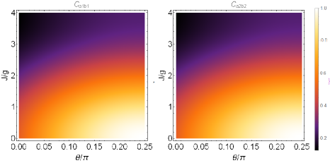
(a)

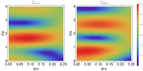
(b)

Figure 5: Bridge qubit coupling. The plots above show the Concurrence for specific pairs of field modes, at time $\tau_{2}=\pi/2$, as a function of $J\equiv J_{1,2}$ and the degree of entanglement of the initial states in cavity $1$ ($\theta$). a) Concurrence relative to the intra-cavity modes, $a_{1}\wedge b_{1}$ and $a_{2}\wedge b_{2}$; b) Concurrence relative to the inter-cavity modes, $a_{1}\wedge b_{2}$, $b_{1}\wedge a_{2}$. The entanglement between modes $a_{1}\wedge a_{2}$ and $b_{1}\wedge b_{2}$, not shown here, features an identical pattern.

We can also look closer at the evolution of entanglement considering an initial preparation in the separable state $|\psi(0)\rangle=|10\rangle_{c1}|g\rangle|00\rangle_{c2}$. Fig. 6 illustrates the evolution of entanglement between the intra-cavity modes of both cavities up to the time $\tau=2\pi$. Note that, unlike the case of having an initial entangled state prepared in cavity $1$, here the entanglement between modes $a_{1}\wedge b_{1}$ (and between modes $a_{2}\wedge b_{2}$) reaches the maximum value of $C=0.5$ at $\tau_{2}=\pi/2$. This happens because precisely at that specific time, all four fields constitute a 4-partite entangled state, leaving the atom separated. As a consequence, the bipartite states formed by the fields in cavity $1$ $(a_{1}\wedge b_{1})$ and in cavity $2$ $(a_{2}\wedge b_{2})$ are each one in a partially entangled state at $\tau_{2}=\pi/2$, with $C=0.5$. We also note that the entanglement evolution in each cavity shows different patterns; in cavity $1$, the maximum entanglement is reached more quickly than in cavity $2$, and it also decays more slowly. We also observe that the entanglement in cavity $1$ is kept at a constant (maximum) value during a significantly large time interval. This resembles the so-called “freezing (and thawing) of entanglement" [30, 31], a phenomenon in which entanglement “freezes" at some particular value during the evolution, decreasing after some time. On the other hand, in cavity $2$ the entanglement between modes $a_{2}\wedge b_{2}$ undergoes SDE, becoming null in a finite time interval around $\tau_{3}=\pi$. Nonetheless, the field modes in cavity $1$ do not suffer SDE. Clearly, the entanglement distribution in the system as well as its “freezing" depend on which subsystem contains the initial field state excitation [30, 31]. If the photon initially populates mode $a_{1}$, entanglement freezing occurs in cavity $1$. Conversely, the modes in cavity $2$ undergo SDE. However, if the photon populates mode $a_{2}$ instead, it will be the other way around, i.e., freezing will occur in in cavity $2$, while SDE will take place in cavity $a_{1}$.

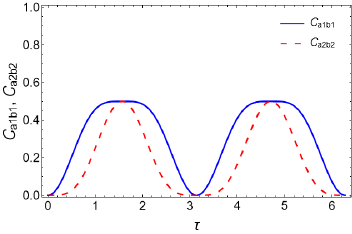
Figure 6: Concurrence as a function of the normalized time $\tau$ (showing “sudden freezing”) relatively to the field modes in cavity $1$ ($a_{1}\wedge b_{1}$) and in cavity $2$ ($a_{2}\wedge b_{2}$) for a bridge qubit coupling, with $g_{1}=g_{2}=g$ and $J_{1}=J_{2}=0$. The initial state of the system is $|{\psi(0)}\rangle=\frac{1}{\sqrt{2}}|10\rangle_{c1}|g\rangle|00\rangle_{c2}$.

3.2.2 Coupling via evanescent waves

In the case of having the cavities connected via evanescent waves, a direct coupling between field modes is established, and we may assume an initial state of the form $|\Phi(0)\rangle=(\cos\theta|10\rangle+\sin\theta|01\rangle)_{c1}|00\rangle_{c2}$, involving only field states. Having the evolution of the system governed by the Hamiltonian in Eq. (4) from an initial product state $(\theta=0)$ and non-interacting intra-cavity modes $(J_{i}=0)$, we find that at $\tau_{1}=\pi/4$ the following entangled state is generated,

$$|\Phi(\tau=\pi/4,\theta=0,J_{1,2}=0)\rangle=\frac{1}{\sqrt{2}}(|1\rangle_{a1}|0\rangle_{b2}+|0\rangle_{a1}|1\rangle_{b2})\otimes|0\rangle_{b1}|0\rangle_{a2},$$ (23)

i.e., a maximally entangled state with modes $a_{1}\wedge b_{2}$. At the same time, the modes $a_{2}\wedge b_{1}$ remain non-entangled. Interestingly, if we switch on the interaction between the intra-cavity modes in the cavities $(J_{1}=J_{2}=2\lambda)$, a different entangled state also involving the modes in both cavities will be formed,

$$|\Phi(\tau=\pi/4,\theta=0,J_{1,2}=2\lambda)\rangle=\frac{1}{\sqrt{2}}(|1\rangle_{b1}|0\rangle_{a2}+|0\rangle_{b1}|1\rangle_{a2})\otimes|0\rangle_{a1}|0\rangle_{b2},$$ (24)

which is a maximally entangled state of modes $a_{2}\wedge b_{1}$, remaining the modes $a_{1}\wedge b_{2}$ non-entangled.

Hence, the generation of specific entangled states between different modes (Eq. (23) and Eq. (24)) can be accomplished simply by tuning the intra-cavity couplings $J_{i}$. We may also calculate the Concurrence by fixing the time, $\tau_{1}=\pi/4$, and varying the couplings $J_{i}$ as well as the weighting angle $\theta$, as shown in Fig. 7. It is clear that the Concurrence is a periodic function of the parameters $J_{i}$, exhibiting different patterns which will depend on the pair of field modes considered. We remark that maximum entanglement $(C=1)$ between modes of distinct cavities is achieved (at $\tau_{1}=\pi/4$) for specific values of the couplings $J_{i}$, namely, for $J_{1,2}=0$ and $J_{1,2}=4\lambda$ in the case of $a_{1}\wedge b_{2}$, and $J_{1,2}=2\lambda$ in the case of $a_{2}\wedge b_{1}$. Moreover, the generation of entanglement is possible from an initial joint product state, and that an initial maximally entangled state in cavity $1$ $(\theta=\pi/4\,\mbox{rad})$ does not result in a maximally state of other modes at $\tau_{1}=\pi/4$. Yet, for each of the remaining bi-partitions ($a_{1}\wedge b_{1}$, $a_{2}\wedge b_{2}$, $a_{1}\wedge a_{2}$, and $b_{1}\wedge b_{2}$), the maximum possible value of the Concurrence is $C=0.5$, irrespective of the values of $J_{i}$ and $\theta$.

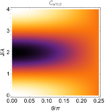
(a)

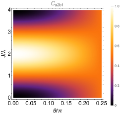
(b)

Figure 7: Evanescent waves coupling. The plots above show the Concurrence for specific pairs of field modes, at $\tau_{1}=\pi/4$, as a function of the $J\equiv J_{1,2}$ coupling and the degree of entanglement of the initial states in cavity $1$ ($\theta$); a) modes $a_{1}\wedge b_{2}$; and b) modes $a_{2}\wedge b_{1}$.

3.3 Coupling via an optical fiber

Another possible way of coupling the microtoroidal cavities is via an optical fiber. We assume the so-called short fiber limit, in which the cavities couple effectively only to a single mode of the fiber, here described by creation and annihilation operators $c^{\dagger}$ and $c$, respectively. The complete Hamiltonian including the fiber reads:

$$H_{T}=H_{S}+H_{\nu},$$ (25)

where

$$H_{\nu}=\hbar\nu\left[(a_{1}^{\dagger}+b_{1}^{\dagger})c+(a_{1}+b_{1})c^{\dagger}+(a_{2}^{\dagger}+b_{2}^{\dagger})c+(a_{2}+b_{2})c^{\dagger}\right]$$ (26)

is the effective interaction term of the cavity modes ($a_{i},b_{i}$) with the fiber mode ($c$) with coupling constant $\nu$. Due to the analogy between the Hamiltonians in Eqs. (3) and (26), equivalent results will be obtained in cavity systems with couplings either via a fiber or via a qubit, provided that the field modes involve only one excitation (one photon).

4 Effects of losses

In order to make a more realistic description of the dynamics of the cavity system, we will now discuss the influence of cavity losses and atomic spontaneous emission on the bipartite entanglement of the intra-cavity field modes. Both effects can be modelled via the usual GKSL-type master equation for the reduced density operator $\rho_{j}\equiv\rho^{(al,bl)}_{j}$ describing the bipartite state relative to the $l$-th cavity

$$\frac{d\rho_{j}}{dt} = -\frac{\textit{i}}{\hbar}[H_{j},\rho_{j}]+\kappa\sum_{i=1,2}\left(2a_{i}\rho_{j}a_{i}^{\dagger}-a_{i}^{\dagger}a_{i}\rho_{j}-\rho_{j}a_{i}^{\dagger}a_{i}\right)$$

$$+ \kappa\sum_{i=1,2}\left(2b_{i}\rho_{j}b_{i}^{\dagger}-b_{i}^{\dagger}b_{i}\rho_{j}-\rho_{j}b_{i}^{\dagger}b_{i}\right)+\gamma\Big{(}2\sigma_{-}\rho_{j}\sigma_{+}-\sigma_{+}\sigma_{-}\rho_{j}-\rho_{j}\sigma_{+}\sigma_{-}\Big{)}.$$

The index $j$ is related to couplings with the qubit $(j=g)$ or via evanescent waves $(j=\lambda)$, respectively. The first term in the right-hand side of Eq. (4) refers to the unitary part, with evolution governed by the Hamiltonian $H_{j}$. The other three terms (Lindbladians) represent the action of external zero temperature reservoirs ($T=0$K) which in general degrade the quantum state properties. For simplicity we assume the same dissipation rate $\kappa$ for each field mode in each of the cavities. In the case of coupling via a qubit, we also take into account the spontaneous emission at a rate $\gamma$, which is typically smaller than $\kappa$ [26]. Of course the last term in Eq. (4) does not exist if the cavities are coupled through evanescent fields. By numerically solving Eq. (4) for the reduced density operator $\rho_{j}$, one may calculate the Concurrence for various bipartite states of cavity fields using Eq. (21). The results will be presented below.

Regarding entanglement transfer, we found that losses have slightly different effects depending on the type of coupling. In Fig. 8(a) we note that although the complete transfer of entanglement from one cavity to another is precluded by losses, the maximum attained entanglement at $\tau_{2}\approx\pi/2$ is larger in the case of coupling via a bridge qubit, compared to the coupling via evanescent waves. This is because the qubit’s spontaneous emission rate is much smaller than the cavity decay rate, and therefore it is less likely a photon to be lost if the cavities are coupled through a qubit rather than via evanescent waves. We recall that for non-zero intra-cavity couplings ($J_{1}=J_{2}\neq 0$), even under ideal conditions the full transfer of entanglement between cavities is not possible if they are coupled by a qubit. The losses of course makes the situation even worse, as shown in Fig. 8(b). In Fig. 9 we have plotted the evolution of Concurrence up to $\tau=2\pi$ to show that, in addition to the expected drop in the maximum values of entanglement, we observe that the time interval in which the entanglement is zero (sudden death), gets a little longer as time passes. The freezing of entanglement will also suffer the effects of losses, as shown in Fig. 10. Interestingly, we notice small entanglement “revivals" around $\tau_{3}=\pi$ (and multiples), that is, at times when the Concurrence is null in the absence of losses.

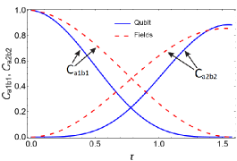
(a)

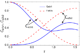
(b)

Figure 8: Effects of losses on quantum entanglement. Concurrence as a function of the normalized time $\tau$ of the cavity $1$ ($a_{1}\wedge b_{1}$) and cavity 2 ($a_{2}\wedge b_{2}$) modes, for couplings via: a bridge qubit (blue line, $\tau^{(g)}$); evanescent fields (dashed red line, $\tau^{(\lambda)}$). The field modes and the qubit are damped at a rate $\kappa=5\times 10^{-2}\eta$ and $\gamma=5\times 10^{-3}\eta$, respectively. For uncoupled intra-cavity modes ($J_{1}=J_{2}=0$) in (a), and coupled modes in (b): $J_{1}=J_{2}=2\eta$. Here $\eta=g$ refers to the bridge qubit coupling, and $\eta=\lambda$ to the coupling via evanescent waves.

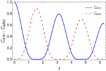
Figure 9: Effects of losses on quantum entanglement. Concurrence as a function of the normalized time $\tau$ relatively to the field modes in cavity $1$ ($a_{1}\wedge b_{1}$) and in cavity $2$ ($a_{2}\wedge b_{2}$) for a bridge qubit coupling, with $g_{1}=g_{2}=g$ and $J_{1}=J_{2}=0$. The field modes and the qubit are damped at a rate $\kappa=5\times 10^{-2}g$ and $\gamma=5\times 10^{-3}g$, respectively. The initial state of the system is $|{\psi(0)}\rangle=\frac{1}{\sqrt{2}}(|10\rangle+|01\rangle)_{c1}|g\rangle|00\rangle_{c2}$.

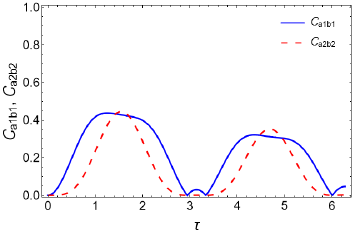
Figure 10: Effects of losses on quantum entanglement. Concurrence as a function of the normalized time $\tau$ relatively to the field modes in cavity $1$ ($a_{1}\wedge b_{1}$) and in cavity $2$ ($a_{2}\wedge b_{2}$) for a bridge qubit coupling, with $g_{1}=g_{2}=g$ and $J_{1}=J_{2}=0$. The field modes and the qubit are damped at a rate $\kappa=5\times 10^{-2}g$ and $\gamma=5\times 10^{-3}g$, respectively. The initial state of the system is $|{\psi(0)}\rangle=\frac{1}{\sqrt{2}}|10\rangle_{c1}|g\rangle|00\rangle_{c2}$.

5 Conclusions

In summary, we have performed a theoretical study demonstrating the experimental feasibility of entanglement generation as well as transfer of maximally entangled states in a system comprising two identical WGMs microtoroidal resonators. We discuss two different types of inter-cavity couplings, that is, using a bridge qubit or via evanescent waves (directly). Firstly we have shown that maximally entangled states of two modes belonging to the same cavity can be transferred with $100\%$ fidelity to the other cavity (in the ideal case). Regarding the generation of entangled states from initial product states, each one of the couplings leads to different entangled states. For instance, we have found that for a evanescent waves coupling, it is allowed the generation of maximally bipartite entangled states (Concurrence $C=1.0$) for modes belonging to different cavities, which manifests the non-local behavior of the resulting quantum states. Besides, we have found that even if the microtoroidal resonators are structurally deformed (leading to $J_{1,2}\neq 0$), it is possible to generate maximally entangled states of pairs of field modes in cavities coupled via evanescent waves. Interestingly, for non-zero intra-cavity couplings, different pairs of field modes become entangled, in comparison to the states generated if $J_{1.2}=0$. Another important result is related to the bridge qubit case, as it allows the generation of a 4-partite state of the cavity fields. Yet despite the fact that the processes of transfer and generation of entanglement are hindered by losses, in the bridge qubit coupling case the field entanglement is more robust against losses when compared to the direct coupling. Thus, the bridge qubit may act both as an assistant of entanglement distribution, as well as an obstacle to entanglement degradation in the two-cavity system. The present study is, therefore, valuable for understanding the several possibilities of transfer and generation of entangled states in two WGMs cavities, depending on how they are coupled, which is certainly relevant for applications in quantum information processing tasks. In particular, the coupling via a bridge qubit turned out to be a very efficient way to distribute entanglement in that system, as well as to generate a unique 4-partite state of all four cavity fields.

References

- [1] N. Gisin, G. Ribordy, W. Tittel, H. Zbinden, Quantum cryptography, Rev. Mod. Phys. 74 (2002) 145–195. doi:10.1103/RevModPhys.74.145.
- [2] E. Diamanti, H.-K. Lo, B. Qi, Z. Yuan, Practical challenges in quantum key distribution, npj Quantum Information 2 (1) (2016) 1–12. doi:10.1038/npjqi.2016.25.
- [3] F. Arute, K. Arya, R. Babbush, D. Bacon, J. C. Bardin, R. Barends, R. Biswas, S. Boixo, F. G. Brandao, D. A. Buell, et al., Quantum supremacy using a programmable superconducting processor, Nature 574 (7779) (2019) 505–510. doi:10.1038/s41586-019-1666-5.
-
[4]
D. Bruß, G. M. D’Ariano, M. Lewenstein, C. Macchiavello, A. Sen(De),
U. Sen,
Distributed
quantum dense coding, Phys. Rev. Lett. 93 (2004) 210501.
doi:10.1103/PhysRevLett.93.210501.
URL https://link.aps.org/doi/10.1103/PhysRevLett.93.210501 - [5] J. Stajic, The future of quantum information processing, Science 339 (6124) (2013) 1163. doi:10.1126/science.339.6124.1163.
- [6] J.-L. Wu, X. Ji, S. Zhang, Fast adiabatic quantum state transfer and entanglement generation between two atoms via dressed states, Scientific reports 7 (1) (2017) 1–11. doi:10.1038/srep46255.
- [7] E. H. Sousa, J. Roversi, Selective engineering for preparing entangled steady states in cavity qed setup, Quantum Reports 1 (1) (2019) 63–70. doi:10.3390/quantum1010007.
- [8] P. J. Blythe, B. T. H. Varcoe, A cavity-QED scheme for cluster-state quantum computing using crossed atomic beams, New Journal of Physics 8 (10) (2006) 231–231. doi:10.1088/1367-2630/8/10/231.
- [9] S. Kato, N. Német, K. Senga, S. Mizukami, X. Huang, S. Parkins, T. Aoki, Observation of dressed states of distant atoms with delocalized photons in coupled-cavities quantum electrodynamics, Nature communications 10 (1) (2019) 1–6. doi:10.1038/s41467-019-08975-8.
- [10] H. J. Kimble, The quantum internet, Nature 453 (7198) (2008) 1023–1030. doi:10.1038/nature07127.
-
[11]
M. Paternostro, W. Son, M. S. Kim, G. Falci, G. M. Palma,
Dynamical
entanglement transfer for quantum-information networks, Phys. Rev. A 70
(2004) 022320.
doi:10.1103/PhysRevA.70.022320.
URL https://link.aps.org/doi/10.1103/PhysRevA.70.022320 -
[12]
S.-L. Ma, Z. Li, A.-P. Fang, P.-B. Li, S.-Y. Gao, F.-L. Li,
Controllable
generation of two-mode-entangled states in two-resonator circuit qed with a
single gap-tunable superconducting qubit, Phys. Rev. A 90 (2014) 062342.
doi:10.1103/PhysRevA.90.062342.
URL https://link.aps.org/doi/10.1103/PhysRevA.90.062342 -
[13]
P.-B. Li, S.-Y. Gao, F.-L. Li,
Engineering
two-mode entangled states between two superconducting resonators by
dissipation, Phys. Rev. A 86 (2012) 012318.
doi:10.1103/PhysRevA.86.012318.
URL https://link.aps.org/doi/10.1103/PhysRevA.86.012318 -
[14]
F. W. Strauch, K. Jacobs, R. W. Simmonds,
Arbitrary
control of entanglement between two superconducting resonators, Phys. Rev.
Lett. 105 (2010) 050501.
doi:10.1103/PhysRevLett.105.050501.
URL https://link.aps.org/doi/10.1103/PhysRevLett.105.050501 -
[15]
F. W. Strauch, D. Onyango, K. Jacobs, R. W. Simmonds,
Entangled-state
synthesis for superconducting resonators, Phys. Rev. A 85 (2012) 022335.
doi:10.1103/PhysRevA.85.022335.
URL https://link.aps.org/doi/10.1103/PhysRevA.85.022335 -
[16]
M. D. Kim, J. Kim,
Coupling qubits in
circuit-qed cavities connected by a bridge qubit, Phys. Rev. A 93 (2016)
012321.
doi:10.1103/PhysRevA.93.012321.
URL https://link.aps.org/doi/10.1103/PhysRevA.93.012321 -
[17]
A. Rauschenbeutel, P. Bertet, S. Osnaghi, G. Nogues, M. Brune, J. M. Raimond,
S. Haroche,
Controlled
entanglement of two field modes in a cavity quantum electrodynamics
experiment, Phys. Rev. A 64 (2001) 050301.
doi:10.1103/PhysRevA.64.050301.
URL https://link.aps.org/doi/10.1103/PhysRevA.64.050301 - [18] X.-H. Wang, R.-Y. Bao, Y.-T. Huang, Two-mode maximally entangled state generated by the microtoroid cavity-atom system, International Journal of Theoretical Physics 50 (2) (2011) 473–478. doi:10.1007/s10773-010-0554-4.
-
[19]
Z. Jin, S. L. Su, S. Zhang,
Preparation of a
steady entangled state of two nitrogen-vacancy centers by simultaneously
utilizing two dissipative factors, Phys. Rev. A 100 (2019) 052332.
doi:10.1103/PhysRevA.100.052332.
URL https://link.aps.org/doi/10.1103/PhysRevA.100.052332 -
[20]
P.-B. Li, S.-Y. Gao, H.-R. Li, S.-L. Ma, F.-L. Li,
Dissipative
preparation of entangled states between two spatially separated
nitrogen-vacancy centers, Phys. Rev. A 85 (2012) 042306.
doi:10.1103/PhysRevA.85.042306.
URL https://link.aps.org/doi/10.1103/PhysRevA.85.042306 - [21] E. H. Sousa, J. Roversi, The role of dipole-dipole interaction and the scattering strength in entanglement dynamics between atoms surrounding a microtoroidal cavity, The European Physical Journal Plus 134 (12) (2019) 607. doi:10.1140/epjp/i2019-13027-y.
-
[22]
X. Yi, Y.-F. Xiao, Y.-C. Liu, B.-B. Li, Y.-L. Chen, Y. Li, Q. Gong,
Multiple-rayleigh-scatterer-induced
mode splitting in a high- whispering-gallery-mode microresonator, Phys.
Rev. A 83 (2011) 023803.
doi:10.1103/PhysRevA.83.023803.
URL https://link.aps.org/doi/10.1103/PhysRevA.83.023803 -
[23]
S. I. Schmid, K. Xia, J. Evers,
Pathway
interference in a loop array of three coupled microresonators, Phys. Rev. A
84 (2011) 013808.
doi:10.1103/PhysRevA.84.013808.
URL https://link.aps.org/doi/10.1103/PhysRevA.84.013808 -
[24]
W. K. Wootters,
Entanglement of
formation of an arbitrary state of two qubits, Phys. Rev. Lett. 80 (1998)
2245–2248.
doi:10.1103/PhysRevLett.80.2245.
URL https://link.aps.org/doi/10.1103/PhysRevLett.80.2245 -
[25]
D. O’Shea, C. Junge, J. Volz, A. Rauschenbeutel,
Fiber-optical
switch controlled by a single atom, Phys. Rev. Lett. 111 (2013) 193601.
doi:10.1103/PhysRevLett.111.193601.
URL https://link.aps.org/doi/10.1103/PhysRevLett.111.193601 -
[26]
B. Dayan, A. S. Parkins, T. Aoki, E. P. Ostby, K. J. Vahala, H. J. Kimble,
A photon
turnstile dynamically regulated by one atom, Science 319 (5866) (2008)
1062–1065.
arXiv:https://science.sciencemag.org/content/319/5866/1062.full.pdf,
doi:10.1126/science.1152261.
URL https://science.sciencemag.org/content/319/5866/1062 -
[27]
K. Życzkowski, P. Horodecki, M. Horodecki,
R. Horodecki,
Dynamics of
quantum entanglement, Phys. Rev. A 65 (2001) 012101.
doi:10.1103/PhysRevA.65.012101.
URL https://link.aps.org/doi/10.1103/PhysRevA.65.012101 -
[28]
T. Yu, J. H. Eberly,
Finite-time
disentanglement via spontaneous emission, Phys. Rev. Lett. 93 (2004) 140404.
doi:10.1103/PhysRevLett.93.140404.
URL https://link.aps.org/doi/10.1103/PhysRevLett.93.140404 -
[29]
G. Deçordi, A. Vidiella-Barranco,
Sudden
death of entanglement induced by a minimal thermal environment, Optics
Communications 475 (2020) 126233.
doi:https://doi.org/10.1016/j.optcom.2020.126233.
URL https://www.sciencedirect.com/science/article/pii/S0030401820306507 -
[30]
M. Ali, A. R. P. Rau,
Sudden change in
dynamics of genuine multipartite entanglement of cavity-reservoir qubits,
Phys. Rev. A 90 (2014) 042330.
doi:10.1103/PhysRevA.90.042330.
URL https://link.aps.org/doi/10.1103/PhysRevA.90.042330 -
[31]
Y. Ding, S. Xie, J. H. Eberly,
Sudden freezing
and thawing of entanglement sharing in a shrunken volume, Phys. Rev. A 103
(2021) 032418.
doi:10.1103/PhysRevA.103.032418.
URL https://link.aps.org/doi/10.1103/PhysRevA.103.032418